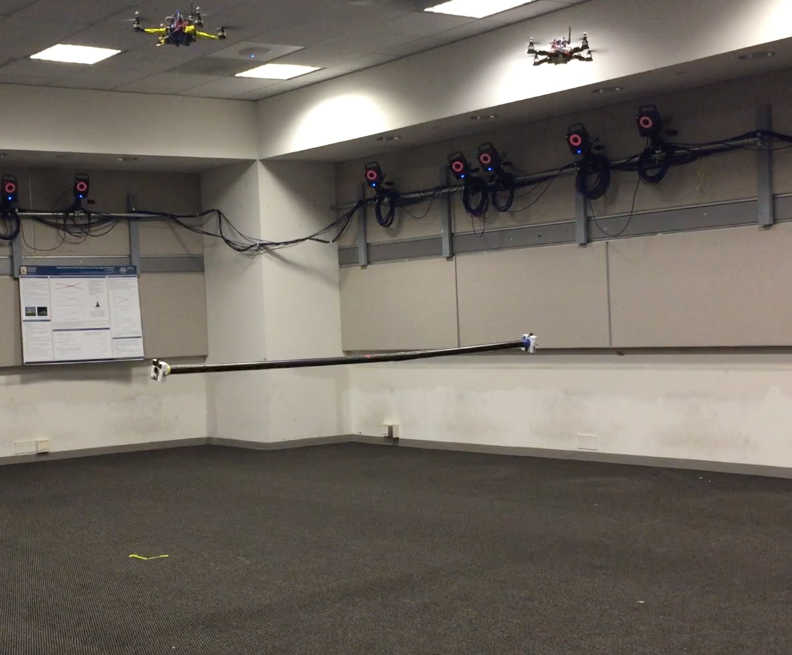
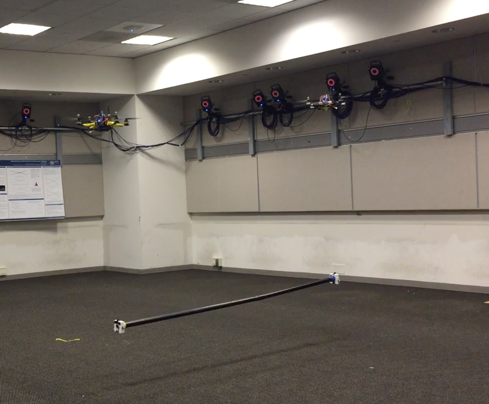
Stabilization of a Rigid Body Payload with Multiple Cooperative Quadrotors

Farhad A. Goodarzi Post Doctoral Fellow
George Washington University
Washington, DC 20052
Email: fgoodarzi@gwu.edu
โ€ƒโ€ƒ Taeyoung Lee Associate Professor
George Washington University
Washington, DC 20052
Email: tylee@gwu.edu
Abstract

This paper presents the full dynamics and control of arbitrary number of quadrotor unmanned aerial vehicles (UAV) transporting a rigid body. The rigid body is connected to the quadrotors via flexible cables where each flexible cable is modeled as a system of arbitrary number of serially-connected links. It is shown that a coordinate-free form of equations of motion can be derived for the complete model without any simplicity assumptions that commonly appear in other literature, according to Lagrangian mechanics on a manifold. A geometric nonlinear controller is presented to transport the rigid body to a fixed desired position while aligning all of the links along the vertical direction. A rigorous mathematical stability proof is given and the desirable features of the proposed controller are illustrated by numerical examples and experimental results.

{nomenclature}\entry

i=1,โ‹ฏ,m๐‘–1โ‹ฏ๐‘ši=1,\cdots,m m number of quadrotors \entrynisubscript๐‘›๐‘–n_{i} Number of links in the i๐‘–i-th cable \entryeโ†’1,eโ†’2,eโ†’3โˆˆโ„3subscriptโ†’๐‘’1subscriptโ†’๐‘’2subscriptโ†’๐‘’3superscriptโ„3\vec{e}_{1},\vec{e}_{2},\vec{e}_{3}\in\mathbb{R}^{3} Inertial frame \entrybโ†’1,bโ†’2,bโ†’3โˆˆโ„3subscriptโ†’๐‘1subscriptโ†’๐‘2subscriptโ†’๐‘3superscriptโ„3\vec{b}_{1},\vec{b}_{2},\vec{b}_{3}\in\mathbb{R}^{3} Body-fixed frame of the payload \entrybโ†’1i,bโ†’2i,bโ†’3iโˆˆโ„3subscriptโ†’๐‘subscript1๐‘–subscriptโ†’๐‘subscript2๐‘–subscriptโ†’๐‘subscript3๐‘–superscriptโ„3\vec{b}_{1_{i}},\vec{b}_{2_{i}},\vec{b}_{3_{i}}\in\mathbb{R}^{3} Body-fixed frame of the i๐‘–i-th quadrotor \entrymiโˆˆโ„subscript๐‘š๐‘–โ„m_{i}\in\mathbb{R} Mass of the i๐‘–i-th quadrotor \entrym0โˆˆโ„subscript๐‘š0โ„m_{0}\in\mathbb{R} Mass of the payload \entryJiโˆˆโ„3ร—3subscript๐ฝ๐‘–superscriptโ„33J_{i}\in\mathbb{R}^{3\times 3} Inertia matrix of the i๐‘–i-th quadrotor \entryRiโˆˆ๐–ฒ๐–ฎโ€‹(๐Ÿฅ)subscript๐‘…๐‘–๐–ฒ๐–ฎ3R_{i}\in\mathsf{SO(3)} Attitude of the i๐‘–i-th quadrotor \entryฮฉiโˆˆโ„3subscriptฮฉ๐‘–superscriptโ„3\Omega_{i}\in\mathbb{R}^{3} Angular velocity of the i๐‘–i-th quadrotor \entryxiโˆˆโ„3subscript๐‘ฅ๐‘–superscriptโ„3x_{i}\in\mathbb{R}^{3} Position of the i๐‘–i-th quadrotor \entryviโˆˆโ„3subscript๐‘ฃ๐‘–superscriptโ„3v_{i}\in\mathbb{R}^{3} Velocity of the i๐‘–i-th quadrotor \entrygโˆˆโ„๐‘”โ„g\in\mathbb{R} Gravitational acceleration \entry๐–ฒ๐–ฎโ€‹(๐Ÿฅ)๐–ฒ๐–ฎ3\mathsf{SO(3)} Special Orthogonal group \entry๐–ฒ๐–คโ€‹(๐Ÿฅ)๐–ฒ๐–ค3\mathsf{SE(3)} Special Euclidean group

1 Introduction

Quadrotor UAVs are being considered for various missions such as Mars surface exploration, search and rescue, and particularly payload transportation. There are various applications for aerial load transportation such as usage in construction, military operations, emergency response, or delivering packages. Load transportation with UAVs can be performed using a cable or by grasping the payloadย [1, 2]. There are several limitations for grasping a payload with UAVs such as in situations where the landing area is inaccessible, or, it transporting a heavy/bulky object by multiple quadrotors.
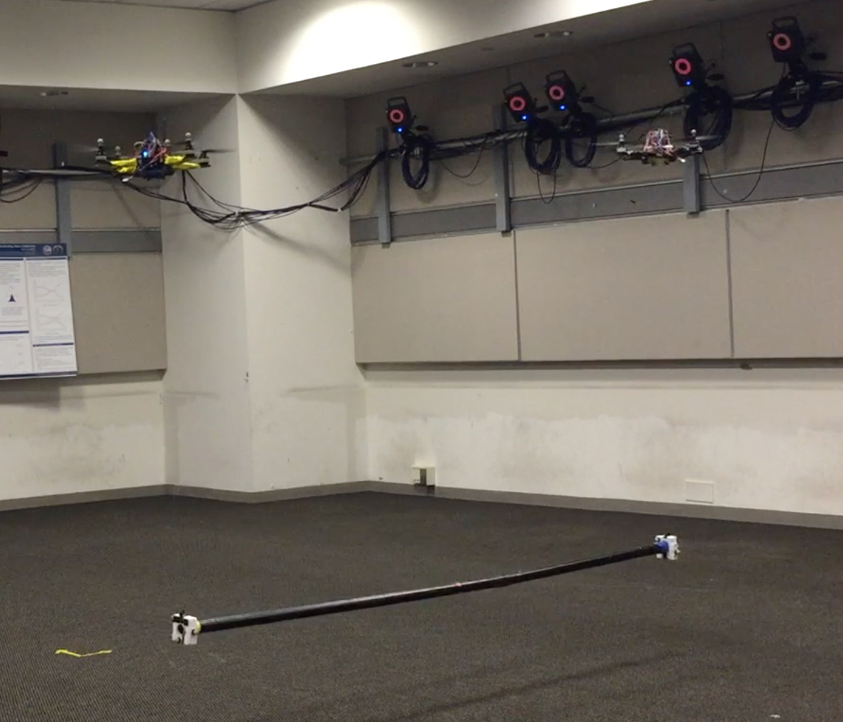
Refer to caption

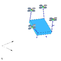
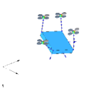
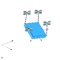
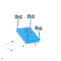
Figure 1: Two quadrotors stabilizing a payload cooperatively.

Load transportation with the cable-suspended load has been studied traditionally for a helicopterย [3, 4] or for small unmanned aerial vehicles such as quadrotor UAVsย [5, 6, 7].

In most of the prior works, the dynamics of aerial transportation has been simplified due to the inherent dynamic complexities. For example, it is assumed that the dynamics of the payload is considered completely decoupled from quadrotors, and the effects of the payload and the cable are regarded as arbitrary external forces and moments exerted to the quadrotorsย [8, 9, 10], thereby making it challenging to suppress the swinging motion of the payload actively, particularly for agile aerial transportations.

Recently, the coupled dynamics of the payload or cable has been explicitly incorporated into control system designย [11]. In particular, a complete model of a quadrotor transporting a payload modeled as a point mass, connected via a flexible cable is presented, where the cable is modeled as serially connected links to represent the deformation of the cableย [12, 13]. In these studies the payload simplified and considered as a point mass without the attitude and the moment of inertia. In another study, multiple quadrotors transporting a rigid body payload has been studiedย [14], but it is assumed that the cables connecting the rigid body payload and quadrotors are always taut. These assumptions and simplifications in the dynamics of the system reduce the stability of the controlled system, particularly in rapid and aggressive load transportation where the motion of the cable and payload is excited nontrivially.

The other critical issue in designing controllers for quadrotors is that they are mostly based on local coordinates. Some aggressive maneuvers are demonstrated atย [15] based on Euler angles. However they involve complicated expressions for trigonometric functions, and they exhibit singularities in representing quadrotor attitudes, thereby restricting their ability to achieve complex rotational maneuvers significantly. A quaternion-based feedback controller for attitude stabilization was shown inย [16]. By considering the Coriolis and gyroscopic torques explicitly, this controller guarantees exponential stability. Quaternions do not have singularities but, as the three-sphere double-covers the special orthogonal group, one attitude may be represented by two antipodal points on the three-sphere. This ambiguity should be carefully resolved in quaternion-based attitude control systems, otherwise they may exhibit unwinding, where a rigid body unnecessarily rotates through a large angle even if the initial attitude error is smallย [17]. To avoid these, an additional mechanism to lift attitude onto the unit-quaternion space is introducedย [18].

Recently, the dynamics of a quadrotor UAV is globally expressed on the special Euclidean group, ๐–ฒ๐–คโ€‹(๐Ÿฅ)๐–ฒ๐–ค3\mathsf{SE(3)}, and nonlinear control systems are developed to track outputs of several flight modesย [19]. There are also several studies using the estimations for dynamical objects developed on the special Euclidean groupย [20, 21]. Several aggressive maneuvers of a quadrotor UAV are demonstrated based on a hybrid control architecture, and a nonlinear robust control system is also considered inย [22, 23]. As they are directly developed on the special Euclidean/Orthogonal group, complexities, singularities, and ambiguities associated with minimal attitude representations or quaternions are completely avoidedย [24, 25]. The proposed control system is particularly useful for rapid and safe payload transportation in complex terrain, where the position of the payload should be controlled concurrently while suppressing the deformation of the cables.

Comparing with the prior work of the authors inย [26, 27, 28] and other existing studies, this paper is the first study considering a complete model which includes a rigid body payload with attitude, arbitrary number of quadrotors, and flexible cables. A rigorous mathematical stability analysis is presented, and numerical and experimental validations in presence of uncertainties and disturbances are provided. More explicitly, we present the complete dynamic model of an arbitrary number of quadrotors transporting a rigid body where each quadrotor is connected to the rigid body via a flexible cable. Each flexible cable is modeled as an arbitrary number of serially connected links, and it is valid for various masses and lengths. A coordinate free form of equations of motion is derived according to Lagrange mechanics on a nonlinear manifold for the full dynamic model. These sets of equations of motion are presented in a complete and organized manner without any restrictive assumption or simplification.

Another contribution of this study is designing a control system to stabilize the rigid body at desired position. Geometric nonlinear controllers presented and generalized for the presented model. More explicitly, we show that the rigid body payload is asymptotically transported into a desired location, while aligning all of the links along the vertical direction corresponding to a hanging equilibrium. This paper presents a rigorous Lyapunov stability analysis for the proposed controller to establish stability properties without any timescale separation assumptions or singular perturbation, and a nonlinear integral control term is designed to guarantee robustness against unstructured uncertainties in both rotational and translational dynamics.

In short, new contributions and the unique features of the dynamics model and control system proposed in this paper compared with other studies are as follows: (i) it is developed for the full dynamic model of arbitrary number of multiple quadrotor UAVs on ๐–ฒ๐–คโ€‹(๐Ÿฅ)๐–ฒ๐–ค3\mathsf{SE(3)} transporting a rigid body connected via flexible cables, including the coupling effects between the translational dynamics and the rotational dynamics on a nonlinear manifold, (ii) the control systems are developed directly on the nonlinear configuration manifold in a coordinate-free fashion. Thus, singularities of local parameterization are completely avoided to generate agile maneuvers in a uniform way, (iii) a rigorous Lyapunov analysis is presented to establish stability properties without any timescale separation assumption, and (iv) an integral control term is proposed to guarantee asymptotical convergence of tracking error variables in the presence of uncertainties, (v) the proposed algorithm is validated with experiments for payload transportation with multiple cooperative quadrotor UAVs. A rigorous and complete mathematical analysis for multiple quadrotor UAVs transporting a payload on ๐–ฒ๐–คโ€‹(๐Ÿฅ)๐–ฒ๐–ค3\mathsf{SE(3)} with experimental validations for payload transportation maneuvers is unprecedented.

This paper is organized as follows. A dynamic model is presented and the problem is formulated at Section II. Control systems are constructed at Sections III and IV, which are followed by numerical examples in Section V. Finally, experimental results are presented in Section VI.

2 Problem Formulation

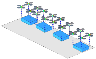
Consider a rigid body with the mass m0โˆˆโ„subscript๐‘š0โ„m_{0}\in\mathbb{R} and the moment of inertia J0โˆˆโ„3ร—3subscript๐ฝ0superscriptโ„33J_{0}\in\mathbb{R}^{3\times 3}, being transported with n๐‘›n arbitrary number of quadrotors as shown in Figureย 2. The location of the mass center of the rigid body is denoted by x0โˆˆโ„3subscript๐‘ฅ0superscriptโ„3x_{0}\in\mathbb{R}^{3}, and its attitude is given by R0โˆˆ๐–ฒ๐–ฎโ€‹(๐Ÿฅ)subscript๐‘…0๐–ฒ๐–ฎ3R_{0}\in\mathsf{SO(3)}, where the special orthogonal group is given by ๐–ฒ๐–ฎโ€‹(๐Ÿฅ)={Rโˆˆโ„3ร—3โˆฃRTโ€‹R=I,det(R)=1}๐–ฒ๐–ฎ3conditional-set๐‘…superscriptโ„33formulae-sequencesuperscript๐‘…๐‘‡๐‘…๐ผ๐‘…1\mathsf{SO(3)}=\{R\in\mathbb{R}^{3\times 3}\mid R^{T}R=I,\det(R)=1\}. We choose an inertial frame {eโ†’1,eโ†’2,eโ†’3}subscriptโ†’๐‘’1subscriptโ†’๐‘’2subscriptโ†’๐‘’3\{\vec{e}_{1},\vec{e}_{2},\vec{e}_{3}\} and body fixed frame {bโ†’1,bโ†’2,bโ†’3}subscriptโ†’๐‘1subscriptโ†’๐‘2subscriptโ†’๐‘3\{\vec{b}_{1},\vec{b}_{2},\vec{b}_{3}\} attached to the payload. We also consider a body fixed frame attached to the i๐‘–i-th quadrotor {bโ†’1i,bโ†’2i,bโ†’3i}subscriptโ†’๐‘subscript1๐‘–subscriptโ†’๐‘subscript2๐‘–subscriptโ†’๐‘subscript3๐‘–\{\vec{b}_{1_{i}},\vec{b}_{2_{i}},\vec{b}_{3_{i}}\}. In the inertial frame, the third axes eโ†’3subscriptโ†’๐‘’3\vec{e}_{3} points downward along the gravity and the other axes are chosen to form an orthonormal frame.

Refer to caption m0subscript๐‘š0m_{0} J0subscript๐ฝ0J_{0} m1subscript๐‘š1m_{1} m1โ€‹jsubscript๐‘š1๐‘—m_{1j} J1subscript๐ฝ1J_{1} m2subscript๐‘š2m_{2} m2โ€‹jsubscript๐‘š2๐‘—m_{2j} J2subscript๐ฝ2J_{2} m3subscript๐‘š3m_{3} m3โ€‹jsubscript๐‘š3๐‘—m_{3j} J3subscript๐ฝ3J_{3} e1subscript๐‘’1e_{1} e2subscript๐‘’2e_{2} e3subscript๐‘’3e_{3} b1subscript๐‘1b_{1} b2subscript๐‘2b_{2} b3subscript๐‘3b_{3}

Figure 2: Quadrotor UAVs with a rigid body payload. Cables are modeled as a serial connection of an arbitrary number of links (only 4 quadrotors with 5 links in each cable are illustrated).

The mass and the moment of inertia of the i๐‘–i-th quadrotor are denoted by miโˆˆโ„subscript๐‘š๐‘–โ„m_{i}\in\mathbb{R} and Jiโˆˆโ„3ร—3subscript๐ฝ๐‘–superscriptโ„33J_{i}\in\mathbb{R}^{3\times 3} respectively. The cable connecting each quadrotor to the rigid body is modeled as an arbitrary numbers of links for each quadrotor with varying masses and lengths. The direction of the j๐‘—j-th link of the i๐‘–i-th quadrotor, measured outward from the quadrotor toward the payload is defined by the unit vector qiโ€‹jโˆˆ๐–ฒ2subscript๐‘ž๐‘–๐‘—superscript๐–ฒ2q_{ij}\in\mathsf{S}^{2}, where ๐–ฒ2={qโˆˆโ„3โˆฃโ€–qโ€–=1}superscript๐–ฒ2conditional-set๐‘žsuperscriptโ„3norm๐‘ž1\mathsf{S}^{2}=\{q\in\mathbb{R}^{3}\mid\|q\|=1\}, where the mass and length of that link is denoted with miโ€‹jsubscript๐‘š๐‘–๐‘—m_{ij} and liโ€‹jsubscript๐‘™๐‘–๐‘—l_{ij} respectively. The number of links in the cable connected to the i๐‘–i-th quadrotor is defined as nisubscript๐‘›๐‘–n_{i}. The configuration manifold for this system is given by ๐–ฒ๐–ฎโ€‹(๐Ÿฅ)ร—โ„3ร—(๐–ฒ๐–ฎโ€‹(๐Ÿฅ)n)ร—(๐–ฒ2)โˆ‘i=1nni๐–ฒ๐–ฎ3superscriptโ„3๐–ฒ๐–ฎsuperscript3๐‘›superscriptsuperscript๐–ฒ2superscriptsubscript๐‘–1๐‘›subscript๐‘›๐‘–\mathsf{SO(3)}\times\mathbb{R}^{3}\times(\mathsf{SO(3)}^{n})\times(\mathsf{S}^{2})^{\sum_{i=1}^{n}n_{i}}.

The i๐‘–i-th quadrotor can generate a thrust force of โˆ’fiโ€‹Riโ€‹e3โˆˆโ„3subscript๐‘“๐‘–subscript๐‘…๐‘–subscript๐‘’3superscriptโ„3-f_{i}R_{i}e_{3}\in\mathbb{R}^{3} with respect to the inertial frame, where fiโˆˆโ„subscript๐‘“๐‘–โ„f_{i}\in\mathbb{R} is the total thrust magnitude of the i๐‘–i-th quadrotor. It also generates a moment Miโˆˆโ„3subscript๐‘€๐‘–superscriptโ„3M_{i}\in\mathbb{R}^{3} with respect to its body-fixed frame. Also we define ฮ”xisubscriptฮ”subscript๐‘ฅ๐‘–\Delta_{x_{i}} and ฮ”Riโˆˆโ„3subscriptฮ”subscript๐‘…๐‘–superscriptโ„3\Delta_{R_{i}}\in\mathbb{R}^{3} as fixed disturbances applied to the i๐‘–i-th quadrotorโ€™s translational and rotational dynamics respectively. It is also assumed that an upper bound of the infinite norm of the uncertainty is known

โ€–ฮ”xโ€–โˆžโ‰คฮด,subscriptnormsubscriptฮ”๐‘ฅ๐›ฟ\displaystyle\|\Delta_{x}\|_{\infty}\leq\delta, (1)

for a positive constant ฮด๐›ฟ\delta. Throughout this paper, the two norm of a matrix A๐ดA is denoted by โ€–Aโ€–norm๐ด\|A\|. The standard dot product is denoted by xโ‹…y=xTโ€‹yโ‹…๐‘ฅ๐‘ฆsuperscript๐‘ฅ๐‘‡๐‘ฆx\cdot y=x^{T}y for any x,yโˆˆโ„3๐‘ฅ๐‘ฆsuperscriptโ„3x,y\in\mathbb{R}^{3}.

2.1 Lagrangian

The kinematics equations for the links, payload, and quadrotors are given by

qห™iโ€‹j=ฯ‰iโ€‹jร—qiโ€‹j=ฯ‰^iโ€‹jโ€‹qiโ€‹j,subscriptห™๐‘ž๐‘–๐‘—subscript๐œ”๐‘–๐‘—subscript๐‘ž๐‘–๐‘—subscript^๐œ”๐‘–๐‘—subscript๐‘ž๐‘–๐‘—\displaystyle\dot{q}_{ij}=\omega_{ij}\times q_{ij}=\hat{\omega}_{ij}q_{ij}, (2)
Rห™0=R0โ€‹ฮฉ^0,subscriptห™๐‘…0subscript๐‘…0subscript^ฮฉ0\displaystyle\dot{R}_{0}=R_{0}\hat{\Omega}_{0}, (3)
Rห™i=Riโ€‹ฮฉ^i,subscriptห™๐‘…๐‘–subscript๐‘…๐‘–subscript^ฮฉ๐‘–\displaystyle\dot{R}_{i}=R_{i}\hat{\Omega}_{i}, (4)

where ฯ‰iโ€‹jโˆˆโ„3subscript๐œ”๐‘–๐‘—superscriptโ„3\omega_{ij}\in\mathbb{R}^{3} is the angular velocity of the j๐‘—j-th link in the i๐‘–i-th cable satisfying qiโ€‹jโ‹…ฯ‰iโ€‹j=0โ‹…subscript๐‘ž๐‘–๐‘—subscript๐œ”๐‘–๐‘—0q_{ij}\cdot\omega_{ij}=0. Also, ฮฉ0โˆˆโ„3subscriptฮฉ0superscriptโ„3\Omega_{0}\in\mathbb{R}^{3} is the angular velocity of the payload and ฮฉiโˆˆโ„3subscriptฮฉ๐‘–superscriptโ„3\Omega_{i}\in\mathbb{R}^{3} is the angular velocity of the i๐‘–i-th quadrotor, expressed with respect to the corresponding body fixed frame. The hat map โ‹…^:โ„3โ†’๐–ฒ๐–ฎโ€‹(๐Ÿฅ):^โ‹…โ†’superscriptโ„3๐–ฒ๐–ฎ3\hat{\cdot}:\mathbb{R}^{3}\rightarrow\mathsf{SO(3)} is defined by the condition that x^โ€‹y=xร—y^๐‘ฅ๐‘ฆ๐‘ฅ๐‘ฆ\hat{x}y=x\times y for all x,yโˆˆโ„3๐‘ฅ๐‘ฆsuperscriptโ„3x,y\in\mathbb{R}^{3}. More explicitly, for a vector a=[a1,a2,a3]Tโˆˆโ„3๐‘Žsuperscriptsubscript๐‘Ž1subscript๐‘Ž2subscript๐‘Ž3๐‘‡superscriptโ„3a=[a_{1},a_{2},a_{3}]^{T}\in\mathbb{R}^{3}, the matrix a^^๐‘Ž\hat{a} is given by

a^=[0โˆ’a3a2a30โˆ’a1โˆ’a2a10].^๐‘Žmatrix0subscript๐‘Ž3subscript๐‘Ž2subscript๐‘Ž30subscript๐‘Ž1subscript๐‘Ž2subscript๐‘Ž10\displaystyle\hat{a}=\begin{bmatrix}0&-a_{3}&a_{2}\\ a_{3}&0&-a_{1}\\ -a_{2}&a_{1}&0\end{bmatrix}. (5)

This identifies the Lie algebra ๐–ฒ๐–ฎโ€‹(๐Ÿฅ)๐–ฒ๐–ฎ3\mathsf{SO(3)} with โ„3superscriptโ„3\mathbb{R}^{3} using the vector cross product in โ„3superscriptโ„3\mathbb{R}^{3}. The inverse of the hat map is denoted by the vee map, โˆจ:๐–ฒ๐–ฎ(๐Ÿฅ)โ†’โ„3\vee:\mathsf{SO(3)}\rightarrow\mathbb{R}^{3}. The position of the i๐‘–i-th quadrotor is given by

xi=x0+R0โ€‹ฯiโˆ’โˆ‘a=1niliโ€‹aโ€‹qiโ€‹a,subscript๐‘ฅ๐‘–subscript๐‘ฅ0subscript๐‘…0subscript๐œŒ๐‘–superscriptsubscript๐‘Ž1subscript๐‘›๐‘–subscript๐‘™๐‘–๐‘Žsubscript๐‘ž๐‘–๐‘Ž\displaystyle x_{i}=x_{0}+R_{0}\rho_{i}-\sum_{a=1}^{n_{i}}{l_{ia}q_{ia}}, (6)

where ฯiโˆˆโ„3subscript๐œŒ๐‘–superscriptโ„3\rho_{i}\in\mathbb{R}^{3} is the vector from the center of mass of the rigid body to the point that i๐‘–i-th cable is connected to the rigid body. Similarly the position of the j๐‘—j-th link in the cable connecting the i๐‘–i-th quadrotor to the rigid body is given by

xiโ€‹j=x0+R0โ€‹ฯiโˆ’โˆ‘a=j+1niliโ€‹aโ€‹qiโ€‹a.subscript๐‘ฅ๐‘–๐‘—subscript๐‘ฅ0subscript๐‘…0subscript๐œŒ๐‘–superscriptsubscript๐‘Ž๐‘—1subscript๐‘›๐‘–subscript๐‘™๐‘–๐‘Žsubscript๐‘ž๐‘–๐‘Ž\displaystyle x_{ij}=x_{0}+R_{0}\rho_{i}-\sum_{a=j+1}^{n_{i}}{l_{ia}q_{ia}}. (7)

We derive equations of motion according to Lagrangian mechanics. Total kinetic energy of the system is given by

T=๐‘‡absent\displaystyle T= 12โ€‹m0โ€‹โ€–xห™0โ€–2+โˆ‘i=1nโˆ‘j=1ni12โ€‹miโ€‹jโ€‹โ€–xห™iโ€‹jโ€–2+12โ€‹โˆ‘i=1nmiโ€‹โ€–xห™iโ€–212subscript๐‘š0superscriptnormsubscriptห™๐‘ฅ02superscriptsubscript๐‘–1๐‘›superscriptsubscript๐‘—1subscript๐‘›๐‘–12subscript๐‘š๐‘–๐‘—superscriptnormsubscriptห™๐‘ฅ๐‘–๐‘—212superscriptsubscript๐‘–1๐‘›subscript๐‘š๐‘–superscriptnormsubscriptห™๐‘ฅ๐‘–2\displaystyle\frac{1}{2}m_{0}\|\dot{x}_{0}\|^{2}+\sum_{i=1}^{n}\sum_{j=1}^{n_{i}}{\frac{1}{2}m_{ij}\|\dot{x}_{ij}\|^{2}}+\frac{1}{2}\sum_{i=1}^{n}{m_{i}\|\dot{x}_{i}\|^{2}}
+12โ€‹โˆ‘i=1nฮฉiโ‹…Jiโ€‹ฮฉi+12โ€‹ฮฉ0โ‹…J0โ€‹ฮฉ0.12superscriptsubscript๐‘–1๐‘›โ‹…subscriptฮฉ๐‘–subscript๐ฝ๐‘–subscriptฮฉ๐‘–โ‹…12subscriptฮฉ0subscript๐ฝ0subscriptฮฉ0\displaystyle+\frac{1}{2}\sum_{i=1}^{n}{\Omega_{i}\cdot J_{i}\Omega_{i}}+\frac{1}{2}\Omega_{0}\cdot J_{0}\Omega_{0}. (8)

The gravitational potential energy is given by

V=โˆ’m0โ€‹gโ€‹e3โ‹…x0โˆ’โˆ‘i=1nmiโ€‹gโ€‹e3โ‹…xiโˆ’โˆ‘i=1nโˆ‘j=1nimiโ€‹jโ€‹gโ€‹e3โ‹…xiโ€‹j,๐‘‰โ‹…subscript๐‘š0๐‘”subscript๐‘’3subscript๐‘ฅ0superscriptsubscript๐‘–1๐‘›โ‹…subscript๐‘š๐‘–๐‘”subscript๐‘’3subscript๐‘ฅ๐‘–superscriptsubscript๐‘–1๐‘›superscriptsubscript๐‘—1subscript๐‘›๐‘–โ‹…subscript๐‘š๐‘–๐‘—๐‘”subscript๐‘’3subscript๐‘ฅ๐‘–๐‘—\displaystyle V=-m_{0}ge_{3}\cdot x_{0}-\sum_{i=1}^{n}{m_{i}ge_{3}}\cdot x_{i}-\sum_{i=1}^{n}\sum_{j=1}^{n_{i}}{m_{ij}ge_{3}}\cdot x_{ij}, (9)

where it is assumed that the unit-vector e3subscript๐‘’3e_{3} points downward along the gravitational acceleration as shown at Figure 2. The corresponding Lagrangian of the system is L=Tโˆ’V๐ฟ๐‘‡๐‘‰L=T-V.

2.2 Euler-Lagrange equations

Coordinate-free form of Lagrangian mechanics on the two-sphere ๐–ฒ2superscript๐–ฒ2\mathsf{S}^{2} and the special orthogonal group ๐–ฒ๐–ฎโ€‹(๐Ÿฅ)๐–ฒ๐–ฎ3\mathsf{SO(3)} for various multi-body systems has been studied inย [29, 30]. The key idea is representing the infinitesimal variation of Riโˆˆ๐–ฒ๐–ฎโ€‹(๐Ÿฅ)subscript๐‘…๐‘–๐–ฒ๐–ฎ3R_{i}\in\mathsf{SO(3)} in terms of the exponential map

ฮดโ€‹Ri=ddโ€‹ฯต|ฯต=0โ€‹Riโ€‹expโก(ฯตโ€‹ฮท^i)=Riโ€‹ฮท^i,๐›ฟsubscript๐‘…๐‘–evaluated-at๐‘‘๐‘‘italic-ฯตitalic-ฯต0subscript๐‘…๐‘–italic-ฯตsubscript^๐œ‚๐‘–subscript๐‘…๐‘–subscript^๐œ‚๐‘–\displaystyle\delta R_{i}=\frac{d}{d\epsilon}\bigg{|}_{\epsilon=0}R_{i}\exp(\epsilon\hat{\eta}_{i})=R_{i}\hat{\eta}_{i}, (10)

for ฮทiโˆˆโ„3subscript๐œ‚๐‘–superscriptโ„3\eta_{i}\in\mathbb{R}^{3}. The corresponding variation of the angular velocity is given by ฮดโ€‹ฮฉi=ฮทห™i+ฮฉiร—ฮทi๐›ฟsubscriptฮฉ๐‘–subscriptห™๐œ‚๐‘–subscriptฮฉ๐‘–subscript๐œ‚๐‘–\delta\Omega_{i}=\dot{\eta}_{i}+\Omega_{i}\times\eta_{i}. Similarly, the infinitesimal variation of qiโ€‹jโˆˆ๐–ฒ2subscript๐‘ž๐‘–๐‘—superscript๐–ฒ2q_{ij}\in\mathsf{S}^{2} is given by

ฮดโ€‹qiโ€‹j=ฮพiโ€‹jร—qiโ€‹j,๐›ฟsubscript๐‘ž๐‘–๐‘—subscript๐œ‰๐‘–๐‘—subscript๐‘ž๐‘–๐‘—\displaystyle\delta q_{ij}=\xi_{ij}\times q_{ij}, (11)

for ฮพiโ€‹jโˆˆโ„3subscript๐œ‰๐‘–๐‘—superscriptโ„3\xi_{ij}\in\mathbb{R}^{3} satisfying ฮพiโ€‹jโ‹…qiโ€‹j=0โ‹…subscript๐œ‰๐‘–๐‘—subscript๐‘ž๐‘–๐‘—0\xi_{ij}\cdot q_{ij}=0. Using these, we obtain the following Euler-Lagrange equations.

Proposition 1

The equations of motion for the proposed payload transportation system are as follows

MTโ€‹xยจ0โˆ’โˆ‘i=1nโˆ‘j=1niM0โ€‹iโ€‹jโ€‹liโ€‹jโ€‹qยจiโ€‹jโˆ’โˆ‘i=1nMiโ€‹Tโ€‹R0โ€‹ฯ^iโ€‹ฮฉห™0subscript๐‘€๐‘‡subscriptยจ๐‘ฅ0superscriptsubscript๐‘–1๐‘›superscriptsubscript๐‘—1subscript๐‘›๐‘–subscript๐‘€0๐‘–๐‘—subscript๐‘™๐‘–๐‘—subscriptยจ๐‘ž๐‘–๐‘—superscriptsubscript๐‘–1๐‘›subscript๐‘€๐‘–๐‘‡subscript๐‘…0subscript^๐œŒ๐‘–subscriptห™ฮฉ0\displaystyle M_{T}\ddot{x}_{0}-\sum_{i=1}^{n}\sum_{j=1}^{n_{i}}{M_{0ij}l_{ij}\ddot{q}_{ij}}-\sum_{i=1}^{n}{M_{iT}R_{0}\hat{\rho}_{i}\dot{\Omega}_{0}}
=MTโ€‹gโ€‹e3+โˆ‘i=1n(โˆ’fiโ€‹Riโ€‹e3+ฮ”xi)โˆ’โˆ‘i=1nMiโ€‹Tโ€‹R0โ€‹ฮฉ^02โ€‹ฯi,absentsubscript๐‘€๐‘‡๐‘”subscript๐‘’3superscriptsubscript๐‘–1๐‘›subscript๐‘“๐‘–subscript๐‘…๐‘–subscript๐‘’3subscriptฮ”subscript๐‘ฅ๐‘–superscriptsubscript๐‘–1๐‘›subscript๐‘€๐‘–๐‘‡subscript๐‘…0superscriptsubscript^ฮฉ02subscript๐œŒ๐‘–\displaystyle=M_{T}ge_{3}+\sum_{i=1}^{n}{(-f_{i}R_{i}e_{3}+\Delta_{x_{i}})}-\sum_{i=1}^{n}{M_{iT}R_{0}\hat{\Omega}_{0}^{2}\rho_{i}}, (12)
Jยฏ0โ€‹ฮฉห™0+โˆ‘i=1nMiโ€‹Tโ€‹ฯ^iโ€‹R0Tโ€‹xยจ0โˆ’โˆ‘i=1nโˆ‘j=1niM0โ€‹iโ€‹jโ€‹liโ€‹jโ€‹ฯ^iโ€‹R0Tโ€‹qยจiโ€‹jsubscriptยฏ๐ฝ0subscriptห™ฮฉ0superscriptsubscript๐‘–1๐‘›subscript๐‘€๐‘–๐‘‡subscript^๐œŒ๐‘–superscriptsubscript๐‘…0๐‘‡subscriptยจ๐‘ฅ0superscriptsubscript๐‘–1๐‘›superscriptsubscript๐‘—1subscript๐‘›๐‘–subscript๐‘€0๐‘–๐‘—subscript๐‘™๐‘–๐‘—subscript^๐œŒ๐‘–superscriptsubscript๐‘…0๐‘‡subscriptยจ๐‘ž๐‘–๐‘—\displaystyle\bar{J}_{0}\dot{\Omega}_{0}+\sum_{i=1}^{n}{M_{iT}\hat{\rho}_{i}R_{0}^{T}\ddot{x}_{0}}-\sum_{i=1}^{n}\sum_{j=1}^{n_{i}}{M_{0ij}l_{ij}\hat{\rho}_{i}R_{0}^{T}\ddot{q}_{ij}}
=โˆ‘i=1nฯ^iโ€‹R0Tโ€‹(โˆ’fiโ€‹Riโ€‹e3+Miโ€‹Tโ€‹gโ€‹e3+ฮ”xi)โˆ’ฮฉ^0โ€‹Jยฏ0โ€‹ฮฉ0,absentsuperscriptsubscript๐‘–1๐‘›subscript^๐œŒ๐‘–superscriptsubscript๐‘…0๐‘‡subscript๐‘“๐‘–subscript๐‘…๐‘–subscript๐‘’3subscript๐‘€๐‘–๐‘‡๐‘”subscript๐‘’3subscriptฮ”subscript๐‘ฅ๐‘–subscript^ฮฉ0subscriptยฏ๐ฝ0subscriptฮฉ0\displaystyle=\sum_{i=1}^{n}{\hat{\rho}_{i}R_{0}^{T}(-f_{i}R_{i}e_{3}+M_{iT}ge_{3}+\Delta_{x_{i}})}-\hat{\Omega}_{0}\bar{J}_{0}\Omega_{0}, (13)
โˆ‘k=1niM0โ€‹iโ€‹jโ€‹liโ€‹kโ€‹q^iโ€‹j2โ€‹qยจiโ€‹kโˆ’M0โ€‹iโ€‹jโ€‹q^iโ€‹j2โ€‹xยจ0+M0โ€‹iโ€‹jโ€‹q^iโ€‹j2โ€‹R0โ€‹ฯ^iโ€‹ฮฉห™0superscriptsubscript๐‘˜1subscript๐‘›๐‘–subscript๐‘€0๐‘–๐‘—subscript๐‘™๐‘–๐‘˜superscriptsubscript^๐‘ž๐‘–๐‘—2subscriptยจ๐‘ž๐‘–๐‘˜subscript๐‘€0๐‘–๐‘—superscriptsubscript^๐‘ž๐‘–๐‘—2subscriptยจ๐‘ฅ0subscript๐‘€0๐‘–๐‘—superscriptsubscript^๐‘ž๐‘–๐‘—2subscript๐‘…0subscript^๐œŒ๐‘–subscriptห™ฮฉ0\displaystyle\sum_{k=1}^{n_{i}}{M_{0ij}l_{ik}\hat{q}_{ij}^{2}\ddot{q}_{ik}}-M_{0ij}\hat{q}_{ij}^{2}\ddot{x}_{0}+M_{0ij}\hat{q}_{ij}^{2}R_{0}\hat{\rho}_{i}\dot{\Omega}_{0}
=M0โ€‹iโ€‹jโ€‹q^iโ€‹j2โ€‹R0โ€‹ฮฉ^02โ€‹ฯiโˆ’q^iโ€‹j2โ€‹(M0โ€‹iโ€‹jโ€‹gโ€‹e3โˆ’fiโ€‹Riโ€‹e3+ฮ”xi),absentsubscript๐‘€0๐‘–๐‘—superscriptsubscript^๐‘ž๐‘–๐‘—2subscript๐‘…0superscriptsubscript^ฮฉ02subscript๐œŒ๐‘–superscriptsubscript^๐‘ž๐‘–๐‘—2subscript๐‘€0๐‘–๐‘—๐‘”subscript๐‘’3subscript๐‘“๐‘–subscript๐‘…๐‘–subscript๐‘’3subscriptฮ”subscript๐‘ฅ๐‘–\displaystyle=M_{0ij}\hat{q}_{ij}^{2}R_{0}\hat{\Omega}_{0}^{2}\rho_{i}-\hat{q}_{ij}^{2}(M_{0ij}ge_{3}-f_{i}R_{i}e_{3}+\Delta_{x_{i}}), (14)
Jiโ€‹ฮฉi+ฮฉiร—Jiโ€‹ฮฉi=Mi+ฮ”Ri.subscript๐ฝ๐‘–subscriptฮฉ๐‘–subscriptฮฉ๐‘–subscript๐ฝ๐‘–subscriptฮฉ๐‘–subscript๐‘€๐‘–subscriptฮ”subscript๐‘…๐‘–\displaystyle J_{i}\Omega_{i}+\Omega_{i}\times J_{i}\Omega_{i}=M_{i}+\Delta_{R_{i}}. (15)

Here the total mass MTsubscript๐‘€๐‘‡M_{T} of the system and the mass of the i๐‘–i-th quadrotor and its flexible cable Miโ€‹Tsubscript๐‘€๐‘–๐‘‡M_{iT} are defined as

MT=m0+โˆ‘i=1nMiโ€‹T,Miโ€‹T=โˆ‘j=1nimiโ€‹j+mi,formulae-sequencesubscript๐‘€๐‘‡subscript๐‘š0superscriptsubscript๐‘–1๐‘›subscript๐‘€๐‘–๐‘‡subscript๐‘€๐‘–๐‘‡superscriptsubscript๐‘—1subscript๐‘›๐‘–subscript๐‘š๐‘–๐‘—subscript๐‘š๐‘–\displaystyle M_{T}=m_{0}+\sum_{i=1}^{n}M_{iT},\;M_{iT}=\sum_{j=1}^{n_{i}}{m_{ij}}+m_{i}, (16)

and the constants related to the mass of links are given as

M0โ€‹iโ€‹jsubscript๐‘€0๐‘–๐‘—\displaystyle M_{0ij} =mi+โˆ‘a=1jโˆ’1miโ€‹a,absentsubscript๐‘š๐‘–superscriptsubscript๐‘Ž1๐‘—1subscript๐‘š๐‘–๐‘Ž\displaystyle=m_{i}+\sum_{a=1}^{j-1}{m_{ia}}, (17)

The equations of motion can be rearranged in a matrix form as follow

๐โ€‹๐—ห™=๐๐ห™๐—๐\displaystyle\mathbf{N}\dot{\mathbf{X}}=\mathbf{P} (18)

where the state vector Xโˆˆโ„DX๐‘‹superscriptโ„subscript๐ท๐‘‹X\in\mathbb{R}^{D_{X}} with DX=6+3โ€‹โˆ‘i=1nnisubscript๐ท๐‘‹63superscriptsubscript๐‘–1๐‘›subscript๐‘›๐‘–D_{X}=6+3\sum_{i=1}^{n}n_{i} is given by

๐—=[xห™0,ฮฉ0,qห™1โ€‹j,qห™2โ€‹j,โ‹ฏ,qห™nโ€‹j]T,๐—superscriptsubscriptห™๐‘ฅ0subscriptฮฉ0subscriptห™๐‘ž1๐‘—subscriptห™๐‘ž2๐‘—โ‹ฏsubscriptห™๐‘ž๐‘›๐‘—๐‘‡\displaystyle\mathbf{X}=[\dot{x}_{0},\;{\Omega}_{0},\;\dot{q}_{1j},\;\dot{q}_{2j},\;\cdots,\;\dot{q}_{nj}]^{T}, (19)

and matrix ๐โˆˆโ„DXร—DX๐superscriptโ„subscript๐ท๐‘‹subscript๐ท๐‘‹\mathbf{N}\in\mathbb{R}^{D_{X}\times D_{X}} is defined as

๐=[MTโ€‹I3๐x0โ€‹ฮฉ0๐x0โ€‹1๐x0โ€‹2โ‹ฏ๐x0โ€‹n๐ฮฉ0โ€‹x0Jยฏ0๐ฮฉ0โ€‹1๐ฮฉ0โ€‹2โ‹ฏ๐ฮฉ0โ€‹n๐1โ€‹x0๐1โ€‹ฮฉ0๐qโ€‹qโ€‹10โ‹ฏ0๐2โ€‹x0๐2โ€‹ฮฉ00๐qโ€‹qโ€‹2โ‹ฏ0โ‹ฎโ‹ฎโ‹ฎโ‹ฎโ‹ฎโ‹ฎ๐nโ€‹x0๐nโ€‹ฮฉ000โ‹ฏ๐qโ€‹qโ€‹n],๐matrixsubscript๐‘€๐‘‡subscript๐ผ3subscript๐subscript๐‘ฅ0subscriptฮฉ0subscript๐subscript๐‘ฅ01subscript๐subscript๐‘ฅ02โ‹ฏsubscript๐subscript๐‘ฅ0๐‘›subscript๐subscriptฮฉ0subscript๐‘ฅ0subscriptยฏ๐ฝ0subscript๐subscriptฮฉ01subscript๐subscriptฮฉ02โ‹ฏsubscript๐subscriptฮฉ0๐‘›subscript๐1subscript๐‘ฅ0subscript๐1subscriptฮฉ0subscript๐๐‘ž๐‘ž10โ‹ฏ0subscript๐2subscript๐‘ฅ0subscript๐2subscriptฮฉ00subscript๐๐‘ž๐‘ž2โ‹ฏ0โ‹ฎโ‹ฎโ‹ฎโ‹ฎโ‹ฎโ‹ฎsubscript๐๐‘›subscript๐‘ฅ0subscript๐๐‘›subscriptฮฉ000โ‹ฏsubscript๐๐‘ž๐‘ž๐‘›\displaystyle\mathbf{N}=\begin{bmatrix}M_{T}I_{3}&\mathbf{N}_{x_{0}\Omega_{0}}&\mathbf{N}_{x_{0}1}&\mathbf{N}_{x_{0}2}&\cdots&\mathbf{N}_{x_{0}n}\\ \mathbf{N}_{\Omega_{0}x_{0}}&\bar{J}_{0}&\mathbf{N}_{\Omega_{0}1}&\mathbf{N}_{\Omega_{0}2}&\cdots&\mathbf{N}_{\Omega_{0}n}\\ \mathbf{N}_{1x_{0}}&\mathbf{N}_{1\Omega_{0}}&\mathbf{N}_{qq1}&0&\cdots&0\\ \mathbf{N}_{2x_{0}}&\mathbf{N}_{2\Omega_{0}}&0&\mathbf{N}_{qq2}&\cdots&0\\ \vdots&\vdots&\vdots&\vdots&\vdots&\vdots\\ \mathbf{N}_{nx_{0}}&\mathbf{N}_{n\Omega_{0}}&0&0&\cdots&\mathbf{N}_{qqn}\end{bmatrix}, (20)

where the sub-matrices are defined as

๐x0โ€‹ฮฉ0=โˆ’โˆ‘i=1nMiโ€‹Tโ€‹R0โ€‹ฯ^i;๐ฮฉ0โ€‹x0=๐Œx0โ€‹ฮฉ0T,formulae-sequencesubscript๐subscript๐‘ฅ0subscriptฮฉ0superscriptsubscript๐‘–1๐‘›subscript๐‘€๐‘–๐‘‡subscript๐‘…0subscript^๐œŒ๐‘–subscript๐subscriptฮฉ0subscript๐‘ฅ0superscriptsubscript๐Œsubscript๐‘ฅ0subscriptฮฉ0๐‘‡\displaystyle\mathbf{N}_{x_{0}\Omega_{0}}=-\sum_{i=1}^{n}{M_{iT}R_{0}\hat{\rho}_{i}};\;\mathbf{N}_{\Omega_{0}x_{0}}=\mathbf{M}_{x_{0}\Omega_{0}}^{T},
๐x0โ€‹i=โˆ’[M0โ€‹iโ€‹1โ€‹liโ€‹1โ€‹I3,M0โ€‹iโ€‹2โ€‹liโ€‹2โ€‹I3,โ‹ฏ,M0โ€‹iโ€‹niโ€‹liโ€‹niโ€‹I3],subscript๐subscript๐‘ฅ0๐‘–subscript๐‘€0๐‘–1subscript๐‘™๐‘–1subscript๐ผ3subscript๐‘€0๐‘–2subscript๐‘™๐‘–2subscript๐ผ3โ‹ฏsubscript๐‘€0๐‘–subscript๐‘›๐‘–subscript๐‘™๐‘–subscript๐‘›๐‘–subscript๐ผ3\displaystyle\mathbf{N}_{x_{0}i}=-[M_{0i1}l_{i1}{I}_{3},\;M_{0i2}l_{i2}{I}_{3},\;\cdots,\;M_{0in_{i}}l_{in_{i}}{I}_{3}],
๐ฮฉ0โ€‹i=โˆ’[M0โ€‹iโ€‹1โ€‹liโ€‹1โ€‹ฯ^iโ€‹R0T,M0โ€‹iโ€‹2โ€‹liโ€‹2โ€‹ฯ^iโ€‹R0T,โ‹ฏ,M0โ€‹iโ€‹niโ€‹liโ€‹niโ€‹ฯ^iโ€‹R0T],subscript๐subscriptฮฉ0๐‘–subscript๐‘€0๐‘–1subscript๐‘™๐‘–1subscript^๐œŒ๐‘–superscriptsubscript๐‘…0๐‘‡subscript๐‘€0๐‘–2subscript๐‘™๐‘–2subscript^๐œŒ๐‘–superscriptsubscript๐‘…0๐‘‡โ‹ฏsubscript๐‘€0๐‘–subscript๐‘›๐‘–subscript๐‘™๐‘–subscript๐‘›๐‘–subscript^๐œŒ๐‘–superscriptsubscript๐‘…0๐‘‡\displaystyle\mathbf{N}_{\Omega_{0}i}=-[M_{0i1}l_{i1}\hat{\rho}_{i}R_{0}^{T},\;M_{0i2}l_{i2}\hat{\rho}_{i}R_{0}^{T},\;\cdots,\;M_{0in_{i}}l_{in_{i}}\hat{\rho}_{i}R_{0}^{T}],
๐iโ€‹x0=โˆ’[M0โ€‹iโ€‹1โ€‹q^iโ€‹12,M0โ€‹iโ€‹2โ€‹q^iโ€‹22,โ‹ฏ,M0โ€‹iโ€‹niโ€‹q^iโ€‹ni2]T,subscript๐๐‘–subscript๐‘ฅ0superscriptsubscript๐‘€0๐‘–1superscriptsubscript^๐‘ž๐‘–12subscript๐‘€0๐‘–2superscriptsubscript^๐‘ž๐‘–22โ‹ฏsubscript๐‘€0๐‘–subscript๐‘›๐‘–superscriptsubscript^๐‘ž๐‘–subscript๐‘›๐‘–2๐‘‡\displaystyle\mathbf{N}_{ix_{0}}=-[M_{0i1}\hat{q}_{i1}^{2},\;M_{0i2}\hat{q}_{i2}^{2},\;\cdots,\;M_{0in_{i}}\hat{q}_{in_{i}}^{2}]^{T},
๐iโ€‹ฮฉ0=[M0โ€‹iโ€‹1โ€‹q^iโ€‹12โ€‹R0โ€‹ฯ^i,M0โ€‹iโ€‹2โ€‹q^iโ€‹22โ€‹R0โ€‹ฯ^i,โ‹ฏ,M0โ€‹iโ€‹niโ€‹q^iโ€‹ni2โ€‹R0โ€‹ฯ^i]T,subscript๐๐‘–subscriptฮฉ0superscriptsubscript๐‘€0๐‘–1superscriptsubscript^๐‘ž๐‘–12subscript๐‘…0subscript^๐œŒ๐‘–subscript๐‘€0๐‘–2superscriptsubscript^๐‘ž๐‘–22subscript๐‘…0subscript^๐œŒ๐‘–โ‹ฏsubscript๐‘€0๐‘–subscript๐‘›๐‘–superscriptsubscript^๐‘ž๐‘–subscript๐‘›๐‘–2subscript๐‘…0subscript^๐œŒ๐‘–๐‘‡\displaystyle\mathbf{N}_{i\Omega_{0}}=[M_{0i1}\hat{q}_{i1}^{2}R_{0}\hat{\rho}_{i},\;M_{0i2}\hat{q}_{i2}^{2}R_{0}\hat{\rho}_{i},\;\cdots,\;M_{0in_{i}}\hat{q}_{in_{i}}^{2}R_{0}\hat{\rho}_{i}]^{T}, (21)

and the sub-matrix ๐qโ€‹qโ€‹iโˆˆโ„3โ€‹niร—3โ€‹nisubscript๐๐‘ž๐‘ž๐‘–superscriptโ„3subscript๐‘›๐‘–3subscript๐‘›๐‘–\mathbf{N}_{qqi}\in\mathbb{R}^{3n_{i}\times 3n_{i}} is given by

๐qโ€‹qโ€‹i=[โˆ’M011โ€‹liโ€‹1โ€‹I3M012โ€‹liโ€‹2โ€‹q^iโ€‹22โ‹ฏM01โ€‹niโ€‹liโ€‹niโ€‹q^iโ€‹ni2M021โ€‹liโ€‹1โ€‹q^iโ€‹12โˆ’M022โ€‹liโ€‹2โ€‹I3โ‹ฏM02โ€‹niโ€‹liโ€‹niโ€‹q^iโ€‹ni2โ‹ฎโ‹ฎโ‹ฎM0โ€‹niโ€‹1โ€‹liโ€‹1โ€‹q^iโ€‹12M0โ€‹niโ€‹2โ€‹liโ€‹2โ€‹q^iโ€‹22โ‹ฏโˆ’M0โ€‹niโ€‹niโ€‹liโ€‹niโ€‹I3].subscript๐๐‘ž๐‘ž๐‘–matrixsubscript๐‘€011subscript๐‘™๐‘–1subscript๐ผ3subscript๐‘€012subscript๐‘™๐‘–2superscriptsubscript^๐‘ž๐‘–22โ‹ฏsubscript๐‘€01subscript๐‘›๐‘–subscript๐‘™๐‘–subscript๐‘›๐‘–superscriptsubscript^๐‘ž๐‘–subscript๐‘›๐‘–2subscript๐‘€021subscript๐‘™๐‘–1superscriptsubscript^๐‘ž๐‘–12subscript๐‘€022subscript๐‘™๐‘–2subscript๐ผ3โ‹ฏsubscript๐‘€02subscript๐‘›๐‘–subscript๐‘™๐‘–subscript๐‘›๐‘–superscriptsubscript^๐‘ž๐‘–subscript๐‘›๐‘–2โ‹ฎโ‹ฎmissing-subexpressionโ‹ฎsubscript๐‘€0subscript๐‘›๐‘–1subscript๐‘™๐‘–1superscriptsubscript^๐‘ž๐‘–12subscript๐‘€0subscript๐‘›๐‘–2subscript๐‘™๐‘–2superscriptsubscript^๐‘ž๐‘–22โ‹ฏsubscript๐‘€0subscript๐‘›๐‘–subscript๐‘›๐‘–subscript๐‘™๐‘–subscript๐‘›๐‘–subscript๐ผ3\displaystyle\mathbf{N}_{qqi}=\begin{bmatrix}-M_{011}l_{i1}I_{3}&M_{012}l_{i2}\hat{q}_{i2}^{2}&\cdots&M_{01n_{i}}l_{in_{i}}\hat{q}_{in_{i}}^{2}\\ M_{021}l_{i1}\hat{q}_{i1}^{2}&-M_{022}l_{i2}I_{3}&\cdots&M_{02n_{i}}l_{in_{i}}\hat{q}_{in_{i}}^{2}\\ \vdots&\vdots&&\vdots\\ M_{0n_{i}1}l_{i1}\hat{q}_{i1}^{2}&M_{0n_{i}2}l_{i2}\hat{q}_{i2}^{2}&\cdots&-M_{0n_{i}n_{i}}l_{in_{i}}I_{3}\end{bmatrix}. (22)

The ๐โˆˆโ„DX๐superscriptโ„subscript๐ท๐‘‹\mathbf{P}\in\mathbb{R}^{D_{X}} matrix is

๐=[Px0,Pฮฉ0,P1โ€‹j,P2โ€‹j,โ‹ฏ,Pnโ€‹j]T,๐superscriptsubscript๐‘ƒsubscript๐‘ฅ0subscript๐‘ƒsubscriptฮฉ0subscript๐‘ƒ1๐‘—subscript๐‘ƒ2๐‘—โ‹ฏsubscript๐‘ƒ๐‘›๐‘—๐‘‡\displaystyle\mathbf{P}=[P_{x_{0}},\;P_{\Omega_{0}},\;P_{1j},\;P_{2j},\;\cdots,\;P_{nj}]^{T}, (23)

and sub-matrices of ๐๐\mathbf{P} matrix are also defined as

Px0subscript๐‘ƒsubscript๐‘ฅ0\displaystyle P_{x_{0}} =MTโ€‹gโ€‹e3+โˆ‘i=1n(โˆ’fiโ€‹Riโ€‹e3+ฮ”xi)โˆ’โˆ‘i=1nMiโ€‹Tโ€‹R0โ€‹ฮฉ^02โ€‹ฯi,absentsubscript๐‘€๐‘‡๐‘”subscript๐‘’3superscriptsubscript๐‘–1๐‘›subscript๐‘“๐‘–subscript๐‘…๐‘–subscript๐‘’3subscriptฮ”subscript๐‘ฅ๐‘–superscriptsubscript๐‘–1๐‘›subscript๐‘€๐‘–๐‘‡subscript๐‘…0superscriptsubscript^ฮฉ02subscript๐œŒ๐‘–\displaystyle=M_{T}ge_{3}+\sum_{i=1}^{n}{(-f_{i}R_{i}e_{3}+\Delta_{x_{i}})}-\sum_{i=1}^{n}{M_{iT}R_{0}\hat{\Omega}_{0}^{2}\rho_{i}},
Pฮฉ0subscript๐‘ƒsubscriptฮฉ0\displaystyle P_{\Omega_{0}} =โˆ’ฮฉ^0โ€‹Jยฏ0โ€‹ฮฉ0+โˆ‘i=1nฯ^iโ€‹R0Tโ€‹(Miโ€‹Tโ€‹gโ€‹e3โˆ’fiโ€‹Riโ€‹e3+ฮ”xi),absentsubscript^ฮฉ0subscriptยฏ๐ฝ0subscriptฮฉ0superscriptsubscript๐‘–1๐‘›subscript^๐œŒ๐‘–superscriptsubscript๐‘…0๐‘‡subscript๐‘€๐‘–๐‘‡๐‘”subscript๐‘’3subscript๐‘“๐‘–subscript๐‘…๐‘–subscript๐‘’3subscriptฮ”subscript๐‘ฅ๐‘–\displaystyle=-\hat{\Omega}_{0}\bar{J}_{0}\Omega_{0}+\sum_{i=1}^{n}{\hat{\rho}_{i}R_{0}^{T}(M_{iT}ge_{3}-f_{i}R_{i}e_{3}+\Delta_{x_{i}})},
Piโ€‹j=subscript๐‘ƒ๐‘–๐‘—absent\displaystyle P_{ij}= โˆ’q^iโ€‹j2โ€‹(โˆ’fiโ€‹Riโ€‹e3+M0โ€‹iโ€‹jโ€‹gโ€‹e3+ฮ”xi)+M0โ€‹iโ€‹jโ€‹q^iโ€‹j2โ€‹R0โ€‹ฮฉ^02โ€‹ฯisuperscriptsubscript^๐‘ž๐‘–๐‘—2subscript๐‘“๐‘–subscript๐‘…๐‘–subscript๐‘’3subscript๐‘€0๐‘–๐‘—๐‘”subscript๐‘’3subscriptฮ”subscript๐‘ฅ๐‘–subscript๐‘€0๐‘–๐‘—superscriptsubscript^๐‘ž๐‘–๐‘—2subscript๐‘…0superscriptsubscript^ฮฉ02subscript๐œŒ๐‘–\displaystyle-\hat{q}_{ij}^{2}(-f_{i}R_{i}e_{3}+M_{0ij}ge_{3}+\Delta_{x_{i}})+M_{0ij}\hat{q}_{ij}^{2}R_{0}\hat{\Omega}_{0}^{2}\rho_{i}
+M0โ€‹iโ€‹jโ€‹โ€–qห™iโ€‹jโ€–2โ€‹qiโ€‹j.subscript๐‘€0๐‘–๐‘—superscriptnormsubscriptห™๐‘ž๐‘–๐‘—2subscript๐‘ž๐‘–๐‘—\displaystyle+M_{0ij}\|\dot{q}_{ij}\|^{2}q_{ij}.
Proof 2.1.

See Appendixย A.

These equations are derived directly on a nonlinear manifold without any simplification. The dynamics of the payload, flexible cables, and quadrotors are considered explicitly, and they avoid singularities and complexities associated to local coordinates.

3 CONTROL SYSTEM DESIGN FOR SIMPLIFIED DYNAMIC MODEL

3.1 Control Problem Formulation

Let x0dโˆˆโ„3subscript๐‘ฅsubscript0๐‘‘superscriptโ„3x_{0_{d}}\in\mathbb{R}^{3} be the desired position of the payload. The desired attitude of the payload is considered as R0d=I3ร—3subscript๐‘…subscript0๐‘‘subscript๐ผ33R_{0_{d}}=I_{3\times 3}, and the desired direction of links is aligned along the vertical direction. The corresponding location of the i๐‘–i-th quadrotor at this desired configuration is given by

xid=x0d+ฯiโˆ’โˆ‘a=1niliโ€‹aโ€‹e3.subscript๐‘ฅsubscript๐‘–๐‘‘subscript๐‘ฅsubscript0๐‘‘subscript๐œŒ๐‘–superscriptsubscript๐‘Ž1subscript๐‘›๐‘–subscript๐‘™๐‘–๐‘Žsubscript๐‘’3\displaystyle x_{i_{d}}=x_{0_{d}}+\rho_{i}-\sum_{a=1}^{n_{i}}{l_{ia}e_{3}}. (24)

We wish to design control forces fisubscript๐‘“๐‘–f_{i} and control moments Misubscript๐‘€๐‘–M_{i} of quadrotors such that this desired configuration becomes asymptotically stable.

3.2 Simplified Dynamic Model

Control forces for each quadrotor is given by โˆ’fiโ€‹Riโ€‹e3subscript๐‘“๐‘–subscript๐‘…๐‘–subscript๐‘’3-f_{i}R_{i}e_{3} for the given equations of motion (12), (13), (14), (15). As such, the quadrotor dynamics is under-actuated. The total thrust magnitude of each quadrotor can be arbitrary chosen, but the direction of the thrust vector is always along the third body fixed axis, represented by Riโ€‹e3subscript๐‘…๐‘–subscript๐‘’3R_{i}e_{3}. But, the rotational attitude dynamics of the quadrotors are fully actuated, and they are not affected by the translational dynamics of the quadrotors or the dynamics of links.

Based on these observations, in this section, we simplify the model by replacing the โˆ’fiโ€‹Riโ€‹e3subscript๐‘“๐‘–subscript๐‘…๐‘–subscript๐‘’3-f_{i}R_{i}e_{3} term by a fictitious control input uiโˆˆโ„3subscript๐‘ข๐‘–superscriptโ„3u_{i}\in\mathbb{R}^{3}, and design an expression for uisubscript๐‘ข๐‘–u_{i} to asymptotically stabilize the desired equilibrium. In other words, we assume that the attitude of the quadrotor can be instantaneously changed. Also ฮ”xisubscriptฮ”subscript๐‘ฅ๐‘–\Delta_{x_{i}} are ignored in the simplified dynamic model. The effects of the attitude dynamics are incorporated at the next section.

3.3 Linear Control System

The control system for the simplified dynamic model is developed based on the linearized equations of motion. At the desired equilibrium, the position and the attitude of the payload are given by x0dsubscript๐‘ฅsubscript0๐‘‘x_{0_{d}} and R0d=I3subscript๐‘…subscript0๐‘‘subscript๐ผ3R_{0_{d}}=I_{3}, respectively. Also, we have qiโ€‹jd=e3subscript๐‘ž๐‘–subscript๐‘—๐‘‘subscript๐‘’3q_{{ij}_{d}}=e_{3} and Rid=I3subscript๐‘…subscript๐‘–๐‘‘subscript๐ผ3R_{i_{d}}=I_{3}. In this equilibrium configuration, the control input for the i๐‘–i-th quadrotor is

uid=โˆ’fidโ€‹Ridโ€‹e3,subscript๐‘ขsubscript๐‘–๐‘‘subscript๐‘“subscript๐‘–๐‘‘subscript๐‘…subscript๐‘–๐‘‘subscript๐‘’3\displaystyle u_{i_{d}}=-f_{i_{d}}R_{i_{d}}e_{3}, (25)

where the total thrust is fid=(Miโ€‹T+m0n)โ€‹gsubscript๐‘“subscript๐‘–๐‘‘subscript๐‘€๐‘–๐‘‡subscript๐‘š0๐‘›๐‘”f_{i_{d}}=(M_{iT}+\frac{m_{0}}{n})g.

The variation of x0subscript๐‘ฅ0x_{0} is given by

ฮดโ€‹x0=x0โˆ’x0d,๐›ฟsubscript๐‘ฅ0subscript๐‘ฅ0subscript๐‘ฅsubscript0๐‘‘\displaystyle\delta x_{0}=x_{0}-x_{0_{d}}, (26)

and the variation of the attitude of the payload is defined as

ฮดโ€‹R0=R0dโ€‹ฮท^0=ฮท^0,๐›ฟsubscript๐‘…0subscript๐‘…subscript0๐‘‘subscript^๐œ‚0subscript^๐œ‚0\displaystyle\delta R_{0}=R_{0_{d}}\hat{\eta}_{0}=\hat{\eta}_{0},

for ฮท0โˆˆโ„3subscript๐œ‚0superscriptโ„3\eta_{0}\in\mathbb{R}^{3}. The variation of qiโ€‹jsubscript๐‘ž๐‘–๐‘—q_{ij} can be written as

ฮดโ€‹qiโ€‹j=ฮพiโ€‹jร—e3,๐›ฟsubscript๐‘ž๐‘–๐‘—subscript๐œ‰๐‘–๐‘—subscript๐‘’3\displaystyle\delta q_{ij}=\xi_{ij}\times e_{3}, (27)

where ฮพiโ€‹jโˆˆโ„3subscript๐œ‰๐‘–๐‘—superscriptโ„3\xi_{ij}\in\mathbb{R}^{3} with ฮพiโ€‹jโ‹…e3=0โ‹…subscript๐œ‰๐‘–๐‘—subscript๐‘’30\xi_{ij}\cdot e_{3}=0. The variation of ฯ‰iโ€‹jsubscript๐œ”๐‘–๐‘—\omega_{ij} is given by ฮดโ€‹ฯ‰iโ€‹jโˆˆโ„3๐›ฟsubscript๐œ”๐‘–๐‘—superscriptโ„3\delta\omega_{ij}\in\mathbb{R}^{3} with ฮดโ€‹ฯ‰iโ€‹jโ‹…e3=0โ‹…๐›ฟsubscript๐œ”๐‘–๐‘—subscript๐‘’30\delta\omega_{ij}\cdot e_{3}=0. Therefore, the third element of each of ฮพiโ€‹jsubscript๐œ‰๐‘–๐‘—\xi_{ij} and ฮดโ€‹ฯ‰iโ€‹j๐›ฟsubscript๐œ”๐‘–๐‘—\delta\omega_{ij} for any equilibrium configuration is zero, and they are omitted in the following linearized equations. The state vector of the linearized equation is composed of CTโ€‹ฮพiโ€‹jโˆˆโ„2superscript๐ถ๐‘‡subscript๐œ‰๐‘–๐‘—superscriptโ„2C^{T}\xi_{ij}\in\mathbb{R}^{2}, where C=[e1,e2]โˆˆโ„3ร—2๐ถsubscript๐‘’1subscript๐‘’2superscriptโ„32C=[e_{1},\;e_{2}]\in\mathbb{R}^{3\times 2}. The variation of the control input ฮดโ€‹uiโˆˆโ„3ร—1๐›ฟsubscript๐‘ข๐‘–superscriptโ„31\delta u_{i}\in\mathbb{R}^{3\times 1}, is given as ฮดโ€‹ui=uiโˆ’uid๐›ฟsubscript๐‘ข๐‘–subscript๐‘ข๐‘–subscript๐‘ขsubscript๐‘–๐‘‘\delta u_{i}=u_{i}-u_{i_{d}}.

Proposition 1.

The linearized equations of the simplified dynamic model are given by

๐Œโ€‹๐ฑยจ+๐†๐ฑ=๐โ€‹ฮดโ€‹u+๐”คโ€‹(๐ฑ,๐ฑห™),๐Œยจ๐ฑ๐†๐ฑ๐๐›ฟ๐‘ข๐”ค๐ฑห™๐ฑ\displaystyle\mathbf{M}\ddot{\mathbf{x}}+\mathbf{G}\mathbf{x}=\mathbf{B}\delta u+\mathfrak{g}(\mathbf{x},\dot{\mathbf{x}}), (28)

where ๐”คโ€‹(๐ฑ,๐ฑห™)๐”ค๐ฑห™๐ฑ\mathfrak{g}(\mathbf{x},\dot{\mathbf{x}}) corresponds to the higher order term and the state vector ๐ฑโˆˆโ„D๐ฑ๐ฑsuperscriptโ„subscript๐ท๐ฑ\mathbf{x}\in\mathbb{R}^{D_{\mathbf{x}}} with D๐ฑ=6+2โ€‹โˆ‘i=1nnisubscript๐ท๐ฑ62superscriptsubscript๐‘–1๐‘›subscript๐‘›๐‘–D_{\mathbf{x}}=6+2\sum_{i=1}^{n}n_{i} is given by

๐ฑ=[ฮดโ€‹x0,ฮท0,CTโ€‹ฮพ1โ€‹j,CTโ€‹ฮพ2โ€‹j,โ‹ฏ,CTโ€‹ฮพnโ€‹j],๐ฑmatrix๐›ฟsubscript๐‘ฅ0subscript๐œ‚0superscript๐ถ๐‘‡subscript๐œ‰1๐‘—superscript๐ถ๐‘‡subscript๐œ‰2๐‘—โ‹ฏsuperscript๐ถ๐‘‡subscript๐œ‰๐‘›๐‘—\displaystyle\mathbf{x}=\begin{bmatrix}\delta{x}_{0},\eta_{0},C^{T}{\xi}_{1j},C^{T}{\xi}_{2j},\cdots,C^{T}{\xi}_{nj}\\ \end{bmatrix},

and ฮดโ€‹u=[ฮดโ€‹u1T,ฮดโ€‹u2T,โ‹ฏ,ฮดโ€‹unT]Tโˆˆโ„3โ€‹nร—1๐›ฟ๐‘ขsuperscript๐›ฟsuperscriptsubscript๐‘ข1๐‘‡๐›ฟsuperscriptsubscript๐‘ข2๐‘‡โ‹ฏ๐›ฟsuperscriptsubscript๐‘ข๐‘›๐‘‡๐‘‡superscriptโ„3๐‘›1\delta u=[\delta u_{1}^{T},\;\delta u_{2}^{T},\;\cdots,\;\delta u_{n}^{T}]^{T}\in\mathbb{R}^{3n\times 1}. The matrix ๐Œโˆˆโ„D๐ฑร—D๐ฑ๐Œsuperscriptโ„subscript๐ท๐ฑsubscript๐ท๐ฑ\mathbf{M}\in\mathbb{R}^{D_{\mathbf{x}}\times D_{\mathbf{x}}} are defined as

๐Œ=[MTโ€‹I3๐Œx0โ€‹ฮฉ0๐Œx0โ€‹1๐Œx0โ€‹2โ‹ฏ๐Œx0โ€‹n๐Œฮฉ0โ€‹x0Jยฏ0๐Œฮฉ0โ€‹1๐Œฮฉ0โ€‹2โ‹ฏ๐Œฮฉ0โ€‹n๐Œ1โ€‹x0๐Œ1โ€‹ฮฉ0๐Œqโ€‹qโ€‹10โ‹ฏ0๐Œ2โ€‹x0๐Œ2โ€‹ฮฉ00๐Œqโ€‹qโ€‹2โ‹ฏ0โ‹ฎโ‹ฎโ‹ฎโ‹ฎโ‹ฎโ‹ฎ๐Œnโ€‹x0๐Œnโ€‹ฮฉ000โ‹ฏ๐Œqโ€‹qโ€‹n],๐Œmatrixsubscript๐‘€๐‘‡subscript๐ผ3subscript๐Œsubscript๐‘ฅ0subscriptฮฉ0subscript๐Œsubscript๐‘ฅ01subscript๐Œsubscript๐‘ฅ02โ‹ฏsubscript๐Œsubscript๐‘ฅ0๐‘›subscript๐Œsubscriptฮฉ0subscript๐‘ฅ0subscriptยฏ๐ฝ0subscript๐Œsubscriptฮฉ01subscript๐Œsubscriptฮฉ02โ‹ฏsubscript๐Œsubscriptฮฉ0๐‘›subscript๐Œ1subscript๐‘ฅ0subscript๐Œ1subscriptฮฉ0subscript๐Œ๐‘ž๐‘ž10โ‹ฏ0subscript๐Œ2subscript๐‘ฅ0subscript๐Œ2subscriptฮฉ00subscript๐Œ๐‘ž๐‘ž2โ‹ฏ0โ‹ฎโ‹ฎโ‹ฎโ‹ฎโ‹ฎโ‹ฎsubscript๐Œ๐‘›subscript๐‘ฅ0subscript๐Œ๐‘›subscriptฮฉ000โ‹ฏsubscript๐Œ๐‘ž๐‘ž๐‘›\displaystyle\mathbf{M}=\begin{bmatrix}M_{T}I_{3}&\mathbf{M}_{x_{0}\Omega_{0}}&\mathbf{M}_{x_{0}1}&\mathbf{M}_{x_{0}2}&\cdots&\mathbf{M}_{x_{0}n}\\ \mathbf{M}_{\Omega_{0}x_{0}}&\bar{J}_{0}&\mathbf{M}_{\Omega_{0}1}&\mathbf{M}_{\Omega_{0}2}&\cdots&\mathbf{M}_{\Omega_{0}n}\\ \mathbf{M}_{1x_{0}}&\mathbf{M}_{1\Omega_{0}}&\mathbf{M}_{qq1}&0&\cdots&0\\ \mathbf{M}_{2x_{0}}&\mathbf{M}_{2\Omega_{0}}&0&\mathbf{M}_{qq2}&\cdots&0\\ \vdots&\vdots&\vdots&\vdots&\vdots&\vdots\\ \mathbf{M}_{nx_{0}}&\mathbf{M}_{n\Omega_{0}}&0&0&\cdots&\mathbf{M}_{qqn}\end{bmatrix},

where the sub-matrices are defined as

๐Œx0โ€‹ฮฉ0=โˆ’โˆ‘i=1nMiโ€‹Tโ€‹ฯ^i;๐Œฮฉ0โ€‹x0=๐Œx0โ€‹ฮฉ0T,formulae-sequencesubscript๐Œsubscript๐‘ฅ0subscriptฮฉ0superscriptsubscript๐‘–1๐‘›subscript๐‘€๐‘–๐‘‡subscript^๐œŒ๐‘–subscript๐Œsubscriptฮฉ0subscript๐‘ฅ0superscriptsubscript๐Œsubscript๐‘ฅ0subscriptฮฉ0๐‘‡\displaystyle\mathbf{M}_{x_{0}\Omega_{0}}=-\sum_{i=1}^{n}{M_{iT}\hat{\rho}_{i}};\quad\mathbf{M}_{\Omega_{0}x_{0}}=\mathbf{M}_{x_{0}\Omega_{0}}^{T},
๐Œx0โ€‹i=[M0โ€‹iโ€‹1โ€‹liโ€‹1โ€‹e^3โ€‹C,M0โ€‹iโ€‹2โ€‹liโ€‹2โ€‹e^3โ€‹C,โ‹ฏ,M0โ€‹iโ€‹niโ€‹liโ€‹niโ€‹e^3โ€‹C],subscript๐Œsubscript๐‘ฅ0๐‘–subscript๐‘€0๐‘–1subscript๐‘™๐‘–1subscript^๐‘’3๐ถsubscript๐‘€0๐‘–2subscript๐‘™๐‘–2subscript^๐‘’3๐ถโ‹ฏsubscript๐‘€0๐‘–subscript๐‘›๐‘–subscript๐‘™๐‘–subscript๐‘›๐‘–subscript^๐‘’3๐ถ\displaystyle\mathbf{M}_{x_{0}i}=[M_{0i1}l_{i1}\hat{e}_{3}C,\;M_{0i2}l_{i2}\hat{e}_{3}C,\;\cdots,\;M_{0in_{i}}l_{in_{i}}\hat{e}_{3}C],
๐Œฮฉ0โ€‹i=[M0โ€‹iโ€‹1โ€‹liโ€‹1โ€‹ฯ^iโ€‹C,M0โ€‹iโ€‹2โ€‹liโ€‹2โ€‹ฯ^iโ€‹C,โ‹ฏ,M0โ€‹iโ€‹niโ€‹liโ€‹niโ€‹ฯ^iโ€‹C],subscript๐Œsubscriptฮฉ0๐‘–subscript๐‘€0๐‘–1subscript๐‘™๐‘–1subscript^๐œŒ๐‘–๐ถsubscript๐‘€0๐‘–2subscript๐‘™๐‘–2subscript^๐œŒ๐‘–๐ถโ‹ฏsubscript๐‘€0๐‘–subscript๐‘›๐‘–subscript๐‘™๐‘–subscript๐‘›๐‘–subscript^๐œŒ๐‘–๐ถ\displaystyle\mathbf{M}_{\Omega_{0}i}=[M_{0i1}l_{i1}\hat{\rho}_{i}C,\;M_{0i2}l_{i2}\hat{\rho}_{i}C,\;\cdots,\;M_{0in_{i}}l_{in_{i}}\hat{\rho}_{i}C],
๐Œiโ€‹x0=โˆ’[M0โ€‹iโ€‹1โ€‹CTโ€‹e^3,M0โ€‹iโ€‹2โ€‹CTโ€‹e^3,โ‹ฏ,M0โ€‹iโ€‹niโ€‹CTโ€‹e^3],subscript๐Œ๐‘–subscript๐‘ฅ0subscript๐‘€0๐‘–1superscript๐ถ๐‘‡subscript^๐‘’3subscript๐‘€0๐‘–2superscript๐ถ๐‘‡subscript^๐‘’3โ‹ฏsubscript๐‘€0๐‘–subscript๐‘›๐‘–superscript๐ถ๐‘‡subscript^๐‘’3\displaystyle\mathbf{M}_{ix_{0}}=-[M_{0i1}C^{T}\hat{e}_{3},\;M_{0i2}C^{T}\hat{e}_{3},\;\cdots,\;M_{0in_{i}}C^{T}\hat{e}_{3}], (29)
๐Œiโ€‹ฮฉ0=[M0โ€‹iโ€‹1โ€‹CTโ€‹e^3โ€‹ฯ^i,M0โ€‹iโ€‹2โ€‹CTโ€‹e^3โ€‹ฯ^i,โ‹ฏ,M0โ€‹iโ€‹niโ€‹CTโ€‹e^3โ€‹ฯ^i],subscript๐Œ๐‘–subscriptฮฉ0subscript๐‘€0๐‘–1superscript๐ถ๐‘‡subscript^๐‘’3subscript^๐œŒ๐‘–subscript๐‘€0๐‘–2superscript๐ถ๐‘‡subscript^๐‘’3subscript^๐œŒ๐‘–โ‹ฏsubscript๐‘€0๐‘–subscript๐‘›๐‘–superscript๐ถ๐‘‡subscript^๐‘’3subscript^๐œŒ๐‘–\displaystyle\mathbf{M}_{i\Omega_{0}}=[M_{0i1}C^{T}\hat{e}_{3}\hat{\rho}_{i},\;M_{0i2}C^{T}\hat{e}_{3}\hat{\rho}_{i},\;\cdots,\;M_{0in_{i}}C^{T}\hat{e}_{3}\hat{\rho}_{i}], (30)

and the sub-matrix ๐Œqโ€‹qโ€‹iโˆˆโ„2โ€‹niร—2โ€‹nisubscript๐Œ๐‘ž๐‘ž๐‘–superscriptโ„2subscript๐‘›๐‘–2subscript๐‘›๐‘–\mathbf{M}_{qqi}\in\mathbb{R}^{2n_{i}\times 2n_{i}} is given by

๐Œqโ€‹qโ€‹i=[Miโ€‹11โ€‹liโ€‹1โ€‹I2Miโ€‹12โ€‹liโ€‹2โ€‹I2โ‹ฏMiโ€‹1โ€‹niโ€‹liโ€‹niโ€‹I2Miโ€‹21โ€‹liโ€‹1โ€‹I2Miโ€‹22โ€‹liโ€‹2โ€‹I2โ‹ฏMiโ€‹2โ€‹niโ€‹liโ€‹niโ€‹I2โ‹ฎโ‹ฎโ‹ฎMiโ€‹niโ€‹1โ€‹liโ€‹1โ€‹I2Miโ€‹niโ€‹2โ€‹liโ€‹2โ€‹I2โ‹ฏMiโ€‹niโ€‹niโ€‹liโ€‹niโ€‹I2].subscript๐Œ๐‘ž๐‘ž๐‘–matrixsubscript๐‘€๐‘–11subscript๐‘™๐‘–1subscript๐ผ2subscript๐‘€๐‘–12subscript๐‘™๐‘–2subscript๐ผ2โ‹ฏsubscript๐‘€๐‘–1subscript๐‘›๐‘–subscript๐‘™๐‘–subscript๐‘›๐‘–subscript๐ผ2subscript๐‘€๐‘–21subscript๐‘™๐‘–1subscript๐ผ2subscript๐‘€๐‘–22subscript๐‘™๐‘–2subscript๐ผ2โ‹ฏsubscript๐‘€๐‘–2subscript๐‘›๐‘–subscript๐‘™๐‘–subscript๐‘›๐‘–subscript๐ผ2โ‹ฎโ‹ฎmissing-subexpressionโ‹ฎsubscript๐‘€๐‘–subscript๐‘›๐‘–1subscript๐‘™๐‘–1subscript๐ผ2subscript๐‘€๐‘–subscript๐‘›๐‘–2subscript๐‘™๐‘–2subscript๐ผ2โ‹ฏsubscript๐‘€๐‘–subscript๐‘›๐‘–subscript๐‘›๐‘–subscript๐‘™๐‘–subscript๐‘›๐‘–subscript๐ผ2\displaystyle\mathbf{M}_{qqi}=\begin{bmatrix}M_{i11}l_{i1}I_{2}&M_{i12}l_{i2}I_{2}&\cdots&M_{i1n_{i}}l_{in_{i}}I_{2}\\ M_{i21}l_{i1}I_{2}&M_{i22}l_{i2}I_{2}&\cdots&M_{i2n_{i}}l_{in_{i}}I_{2}\\ \vdots&\vdots&&\vdots\\ M_{in_{i}1}l_{i1}I_{2}&M_{in_{i}2}l_{i2}I_{2}&\cdots&M_{in_{i}n_{i}}l_{in_{i}}I_{2}\end{bmatrix}. (31)

The matrix ๐†โˆˆโ„D๐ฑร—D๐ฑ๐†superscriptโ„subscript๐ท๐ฑsubscript๐ท๐ฑ\mathbf{G}\in\mathbb{R}^{D_{\mathbf{x}}\times D_{\mathbf{x}}} is defined as

๐†=[0000000๐†ฮฉ0โ€‹ฮฉ0000000๐†1000000๐†200โ‹ฎโ‹ฎโ‹ฎโ‹ฎโ‹ฎโ‹ฎ00000๐†n],๐†matrix0000000subscript๐†subscriptฮฉ0subscriptฮฉ0000000subscript๐†1000000subscript๐†200โ‹ฎโ‹ฎโ‹ฎโ‹ฎโ‹ฎโ‹ฎ00000subscript๐†๐‘›\displaystyle\mathbf{G}=\begin{bmatrix}0&0&0&0&0&0\\ 0&\mathbf{G}_{\Omega_{0}\Omega_{0}}&0&0&0&0\\ 0&0&\mathbf{G}_{1}&0&0&0\\ 0&0&0&\mathbf{G}_{2}&0&0\\ \vdots&\vdots&\vdots&\vdots&\vdots&\vdots\\ 0&0&0&0&0&\mathbf{G}_{n}\end{bmatrix},

where ๐†ฮฉ0โ€‹ฮฉ0=โˆ‘i=1nm0nโ€‹gโ€‹ฯ^iโ€‹e^3subscript๐†subscriptฮฉ0subscriptฮฉ0superscriptsubscript๐‘–1๐‘›subscript๐‘š0๐‘›๐‘”subscript^๐œŒ๐‘–subscript^๐‘’3\mathbf{G}_{\Omega_{0}\Omega_{0}}=\sum_{i=1}^{n}\frac{m_{0}}{n}g\hat{\rho}_{i}\hat{e}_{3} and the sub-matrices ๐†iโˆˆโ„2โ€‹niร—2โ€‹nisubscript๐†๐‘–superscriptโ„2subscript๐‘›๐‘–2subscript๐‘›๐‘–\mathbf{G}_{i}\in\mathbb{R}^{2n_{i}\times 2n_{i}} are

๐†i=diag[(โˆ’Miโ€‹Tโˆ’m0n+M0โ€‹iโ€‹j)โ€‹gโ€‹e3โ€‹I2].subscript๐†๐‘–diagdelimited-[]subscript๐‘€๐‘–๐‘‡subscript๐‘š0๐‘›subscript๐‘€0๐‘–๐‘—๐‘”subscript๐‘’3subscript๐ผ2\displaystyle\mathbf{G}_{i}=\mathop{\mathrm{diag}}[(-M_{iT}-\frac{m_{0}}{n}+M_{0ij})ge_{3}I_{2}].

The matrix ๐โˆˆโ„D๐ฑร—3โ€‹n๐superscriptโ„subscript๐ท๐ฑ3๐‘›\mathbf{B}\in\mathbb{R}^{D_{\mathbf{x}}\times 3n} is given by

๐=[I3I3โ‹ฏI3ฯ^1ฯ^2โ‹ฏฯ^n๐๐0000๐๐00โ‹ฎโ‹ฎโ‹ฎโ‹ฎ000๐๐],๐matrixsubscript๐ผ3subscript๐ผ3โ‹ฏsubscript๐ผ3subscript^๐œŒ1subscript^๐œŒ2โ‹ฏsubscript^๐œŒ๐‘›subscript๐๐0000subscript๐๐00โ‹ฎโ‹ฎโ‹ฎโ‹ฎ000subscript๐๐\displaystyle\mathbf{B}=\begin{bmatrix}I_{3}&I_{3}&\cdots&I_{3}\\ \hat{\rho}_{1}&\hat{\rho}_{2}&\cdots&\hat{\rho}_{n}\\ \mathbf{B}_{\mathbf{B}}&0&0&0\\ 0&\mathbf{B}_{\mathbf{B}}&0&0\\ \vdots&\vdots&\vdots&\vdots\\ 0&0&0&\mathbf{B}_{\mathbf{B}}\end{bmatrix},

where ๐๐=โˆ’[CTโ€‹e^3,CTโ€‹e^3,โ‹ฏ,CTโ€‹e^3]Tsubscript๐๐superscriptsuperscript๐ถ๐‘‡subscript^๐‘’3superscript๐ถ๐‘‡subscript^๐‘’3โ‹ฏsuperscript๐ถ๐‘‡subscript^๐‘’3๐‘‡\mathbf{B}_{\mathbf{B}}=-[C^{T}\hat{e}_{3},\;C^{T}\hat{e}_{3},\;\cdots,\;C^{T}\hat{e}_{3}]^{T}.

Proof 3.1.

See Appendixย B.

We present the following PD-type control system for the linearized dynamics

ฮดโ€‹ui=๐›ฟsubscript๐‘ข๐‘–absent\displaystyle\delta u_{i}= โˆ’Kxiโ€‹๐ฑโˆ’Kxห™iโ€‹๐ฑห™,subscript๐พsubscript๐‘ฅ๐‘–๐ฑsubscript๐พsubscriptห™๐‘ฅ๐‘–ห™๐ฑ\displaystyle-K_{x_{i}}\mathbf{x}-K_{\dot{x}_{i}}\dot{\mathbf{x}}, (32)

for controller gains Kxi,Kxห™iโˆˆโ„3ร—D๐ฑsubscript๐พsubscript๐‘ฅ๐‘–subscript๐พsubscriptห™๐‘ฅ๐‘–superscriptโ„3subscript๐ท๐ฑK_{x_{i}},K_{\dot{x}_{i}}\in\mathbb{R}^{3\times D_{\mathbf{x}}}. Provided that (28) is controllable, we can choose the combined controller gains K๐ฑ=[Kx1T,โ€ฆโ€‹KxnT]Tsubscript๐พ๐ฑsuperscriptsuperscriptsubscript๐พsubscript๐‘ฅ1๐‘‡โ€ฆsuperscriptsubscript๐พsubscript๐‘ฅ๐‘›๐‘‡๐‘‡K_{\mathbf{x}}=[K_{x_{1}}^{T},\,\ldots\;K_{x_{n}}^{T}]^{T}, K๐ฑห™=[Kxห™1T,โ€ฆโ€‹Kxห™nT]Tโˆˆโ„3โ€‹nร—D๐ฑsubscript๐พห™๐ฑsuperscriptsuperscriptsubscript๐พsubscriptห™๐‘ฅ1๐‘‡โ€ฆsuperscriptsubscript๐พsubscriptห™๐‘ฅ๐‘›๐‘‡๐‘‡superscriptโ„3๐‘›subscript๐ท๐ฑK_{\dot{\mathbf{x}}}=[K_{\dot{x}_{1}}^{T},\,\ldots K_{\dot{x}_{n}}^{T}]^{T}\in\mathbb{R}^{3n\times D_{\mathbf{x}}} such that the equilibrium is asymptotically stable for the linearized equationsย [31]. Then, the equilibrium becomes asymptotically stable for the nonlinear Euler-Lagrange equation. The controlled linearized system can be written as

zห™1=๐”ธโ€‹z1+๐”นโ€‹(๐โ€‹X+๐”คโ€‹(๐ฑ,๐ฑห™)),subscriptห™๐‘ง1๐”ธsubscript๐‘ง1๐”น๐๐‘‹๐”ค๐ฑห™๐ฑ\displaystyle\dot{z}_{1}=\mathds{A}z_{1}+\mathds{B}(\mathbf{B}X+\mathfrak{g}(\mathbf{x},\dot{\mathbf{x}})), (33)

where z1=[๐ฑ,๐ฑห™]Tโˆˆโ„2โ€‹D๐ฑsubscript๐‘ง1superscript๐ฑห™๐ฑ๐‘‡superscriptโ„2subscript๐ท๐ฑz_{1}=[\mathbf{x},\dot{\mathbf{x}}]^{T}\in\mathbb{R}^{2D_{\mathbf{x}}} and

๐”ธ=[0Iโˆ’๐Œโˆ’1โ€‹(๐†+๐โ€‹K๐ฑ)โˆ’๐Œโˆ’1โ€‹๐โ€‹K๐ฑห™],๐”น=[0๐Œโˆ’1].formulae-sequence๐”ธmatrix0๐ผsuperscript๐Œ1๐†๐subscript๐พ๐ฑsuperscript๐Œ1๐subscript๐พห™๐ฑ๐”นmatrix0superscript๐Œ1\displaystyle\mathds{A}=\begin{bmatrix}0&I\\ -\mathbf{M}^{-1}(\mathbf{G}+\mathbf{B}K_{\mathbf{x}})&-\mathbf{M}^{-1}\mathbf{B}K_{\dot{\mathbf{x}}}\end{bmatrix},\mathds{B}=\begin{bmatrix}0\\ \mathbf{M}^{-1}\end{bmatrix}. (34)

We can also choose K๐ฑsubscript๐พ๐ฑK_{\mathbf{x}} and K๐ฑห™subscript๐พห™๐ฑK_{\dot{\mathbf{x}}} such that ๐”ธโˆˆโ„2โ€‹Dxร—2โ€‹Dx๐”ธsuperscriptโ„2subscript๐ท๐‘ฅ2subscript๐ท๐‘ฅ\mathds{A}\in\mathbb{R}^{2D_{x}\times 2D_{x}} is Hurwitz. Then for any positive definite matrix Qโˆˆโ„2โ€‹D๐ฑร—2โ€‹D๐ฑ๐‘„superscriptโ„2subscript๐ท๐ฑ2subscript๐ท๐ฑQ\in\mathbb{R}^{2D_{\mathbf{x}}\times 2D_{\mathbf{x}}}, there exist a positive definite and symmetric matrix Pโˆˆโ„2โ€‹D๐ฑร—2โ€‹D๐ฑ๐‘ƒsuperscriptโ„2subscript๐ท๐ฑ2subscript๐ท๐ฑP\in\mathbb{R}^{2D_{\mathbf{x}}\times 2D_{\mathbf{x}}} such that ๐”ธTโ€‹P+Pโ€‹๐”ธ=โˆ’Qsuperscript๐”ธ๐‘‡๐‘ƒ๐‘ƒ๐”ธ๐‘„\mathds{A}^{T}P+P\mathds{A}=-Q according toย [31, Thm 3.6].

4 CONTROL SYSTEM DESIGN FOR THE FULL DYNAMIC MODEL

The control system designed at the previous section is based on a simplifying assumption that each quadrotor can generates a thrust along any direction. In the full dynamic model, the direction of the thrust for each quadrotor is parallel to its third body-fixed axis always. In this section, the attitude of each quadrotor is controlled such that the third body-fixed axis becomes parallel to the direction of the ideal control force designed in the previous section. Also in the full dynamics model, we considers the ฮ”xisubscriptฮ”subscript๐‘ฅ๐‘–\Delta_{x_{i}} in the control design and introduce a new integral term to eliminate the disturbances and uncertainties. The central idea is that the attitude Risubscript๐‘…๐‘–R_{i} of the quadrotor is controlled such that its total thrust direction โˆ’Riโ€‹e3subscript๐‘…๐‘–subscript๐‘’3-R_{i}e_{3}, corresponding to the third body-fixed axis, asymptotically follows the direction of the fictitious control input uisubscript๐‘ข๐‘–u_{i}. By choosing the total thrust magnitude properly, we can guarantee asymptotical stability for the full dynamic model.

Let Aiโˆˆโ„3subscript๐ด๐‘–superscriptโ„3A_{i}\in\mathbb{R}^{3} be the ideal total thrust of the i๐‘–i-th quadrotor that asymptotically stabilize the desired equilibrium. Therefor, we have

Ai=uid+ฮดโ€‹ui=โˆ’Kxiโ€‹๐ฑโˆ’Kxห™iโ€‹๐ฑห™โˆ’Kzโ€‹satฯƒ(e๐ฑ)+uid,subscript๐ด๐‘–subscript๐‘ขsubscript๐‘–๐‘‘๐›ฟsubscript๐‘ข๐‘–subscript๐พsubscript๐‘ฅ๐‘–๐ฑsubscript๐พsubscriptห™๐‘ฅ๐‘–ห™๐ฑsubscript๐พ๐‘งsubscriptsat๐œŽsubscript๐‘’๐ฑsubscript๐‘ขsubscript๐‘–๐‘‘\displaystyle A_{i}=u_{i_{d}}+\delta u_{i}=-K_{x_{i}}\mathbf{x}-K_{\dot{x}_{i}}\dot{\mathbf{x}}-K_{z}\mathop{\mathrm{sat}}_{\sigma}(e_{\mathbf{x}})+u_{i_{d}}, (35)

where fidโˆˆโ„subscript๐‘“subscript๐‘–๐‘‘โ„f_{i_{d}}\in\mathbb{R} and uidโˆˆโ„3subscript๐‘ขsubscript๐‘–๐‘‘superscriptโ„3u_{i_{d}}\in\mathbb{R}^{3} are the total thrust and control input of each quadrotor at its equilibrium respectively. where the following integral term e๐ฑโˆˆโ„Dxsubscript๐‘’๐ฑsuperscriptโ„subscript๐ท๐‘ฅe_{\mathbf{x}}\in\mathbb{R}^{D_{x}} is added to eliminate the effect of disturbance ฮ”xisubscriptฮ”subscript๐‘ฅ๐‘–\Delta_{x_{i}} in the full dynamic model

e๐ฑ=โˆซ0t(Pโ€‹๐”น)Tโ€‹z1โ€‹(ฯ„)โ€‹๐‘‘ฯ„,subscript๐‘’๐ฑsubscriptsuperscript๐‘ก0superscript๐‘ƒ๐”น๐‘‡subscript๐‘ง1๐œdifferential-d๐œ\displaystyle e_{\mathbf{x}}=\int^{t}_{0}{(P\mathds{B})^{T}z_{1}(\tau)\;d\tau}, (36)

where Kz=[kzโ€‹I3,kzโ€‹I3,kz1โ€‹I3ร—2,โ€ฆโ€‹kznโ€‹I3ร—2]โˆˆโ„3ร—Dxsubscript๐พ๐‘งsubscript๐‘˜๐‘งsubscript๐ผ3subscript๐‘˜๐‘งsubscript๐ผ3subscript๐‘˜subscript๐‘ง1subscript๐ผ32โ€ฆsubscript๐‘˜subscript๐‘ง๐‘›subscript๐ผ32superscriptโ„3subscript๐ท๐‘ฅK_{z}=[k_{z}I_{3},k_{z}I_{3},k_{z_{1}}I_{3\times 2},\ldots k_{z_{n}}I_{3\times 2}]\in\mathbb{R}^{3\times D_{x}} is an integral gain. For a positive constant ฯƒโˆˆโ„๐œŽโ„\sigma\in\mathbb{R}, a saturation function satฯƒ:โ„โ†’[โˆ’ฯƒ,ฯƒ]:subscriptsat๐œŽโ†’โ„๐œŽ๐œŽ\mathop{\mathrm{sat}}_{\sigma}:\mathbb{R}\rightarrow[-\sigma,\sigma] is introduced as

satฯƒ(y)={ฯƒifย โ€‹y>ฯƒyifย โˆ’ฯƒโ‰คyโ‰คฯƒโˆ’ฯƒifย โ€‹y<โˆ’ฯƒ.subscriptsat๐œŽ๐‘ฆcases๐œŽifย ๐‘ฆ๐œŽ๐‘ฆifย ๐œŽ๐‘ฆ๐œŽ๐œŽifย ๐‘ฆ๐œŽ\displaystyle\mathop{\mathrm{sat}}_{\sigma}(y)=\begin{cases}\sigma&\mbox{if }y>\sigma\\ y&\mbox{if }-\sigma\leq y\leq\sigma\\ -\sigma&\mbox{if }y<-\sigma\\ \end{cases}.

If the input is a vector yโˆˆโ„n๐‘ฆsuperscriptโ„๐‘›y\in\mathbb{R}^{n}, then the above saturation function is applied element by element to define a saturation function satฯƒ(y):โ„nโ†’[โˆ’ฯƒ,ฯƒ]n:subscriptsat๐œŽ๐‘ฆโ†’superscriptโ„๐‘›superscript๐œŽ๐œŽ๐‘›\mathop{\mathrm{sat}}_{\sigma}(y):\mathbb{R}^{n}\rightarrow[-\sigma,\sigma]^{n} for a vector. From the desired direction of the third body-fixed axis of the i๐‘–i-th quadrotor, namely b3iโˆˆ๐–ฒ2subscript๐‘subscript3๐‘–superscript๐–ฒ2b_{3_{i}}\in\mathsf{S}^{2}, is given by

b3i=โˆ’Aiโ€–Aiโ€–.subscript๐‘subscript3๐‘–subscript๐ด๐‘–normsubscript๐ด๐‘–\displaystyle b_{3_{i}}=-\frac{A_{i}}{\|A_{i}\|}. (37)

This provides a two-dimensional constraint on the three dimensional desired attitude of each quadrotor, such that there remains one degree of freedom. To resolve it, the desired direction of the first body-fixed axis b1iโ€‹(t)โˆˆ๐–ฒ2subscript๐‘subscript1๐‘–๐‘กsuperscript๐–ฒ2b_{1_{i}}(t)\in\mathsf{S}^{2} is introduced as a smooth function of time. Due to the fact that the first body-fixed axis is normal to the third body-fixed axis, it is impossible to follow an arbitrary command b1iโ€‹(t)subscript๐‘subscript1๐‘–๐‘กb_{1_{i}}(t) exactly. Instead, its projection onto the plane normal to b3isubscript๐‘subscript3๐‘–b_{3_{i}} is followed, and the desired direction of the second body-fixed axis is chosen to constitute an orthonormal frameย [27]. More explicitly, the desired attitude of the i๐‘–i-th quadrotor is given by

Ric=[โˆ’(b^3i)2โ€‹b1iโ€–(b^3i)2โ€‹b1iโ€–b^3iโ€‹b1iโ€–b^3iโ€‹b1iโ€–b3i],subscript๐‘…subscript๐‘–๐‘matrixsuperscriptsubscript^๐‘subscript3๐‘–2subscript๐‘subscript1๐‘–normsuperscriptsubscript^๐‘subscript3๐‘–2subscript๐‘subscript1๐‘–subscript^๐‘subscript3๐‘–subscript๐‘subscript1๐‘–normsubscript^๐‘subscript3๐‘–subscript๐‘subscript1๐‘–subscript๐‘subscript3๐‘–\displaystyle R_{i_{c}}=\begin{bmatrix}-\frac{(\hat{b}_{3_{i}})^{2}b_{1_{i}}}{\|(\hat{b}_{3_{i}})^{2}b_{1_{i}}\|}&\frac{\hat{b}_{3_{i}}b_{1_{i}}}{\|\hat{b}_{3_{i}}b_{1_{i}}\|}&b_{3_{i}}\end{bmatrix}, (38)

which is guaranteed to be an element of ๐–ฒ๐–ฎโ€‹(๐Ÿฅ)๐–ฒ๐–ฎ3\mathsf{SO(3)}. The desired angular velocity is obtained from the attitude kinematics equation, ฮฉic=(RicTโ€‹Rห™ic)โˆจโˆˆโ„3subscriptฮฉsubscript๐‘–๐‘superscriptsuperscriptsubscript๐‘…subscript๐‘–๐‘๐‘‡subscriptห™๐‘…subscript๐‘–๐‘superscriptโ„3\Omega_{i_{c}}=(R_{i_{c}}^{T}\dot{R}_{i_{c}})^{\vee}\in\mathbb{R}^{3}.

Define the tracking error vectors for the attitude and the angular velocity of the i๐‘–i-th quadrotor as

eRi=12โ€‹(RicTโ€‹Riโˆ’RiTโ€‹Ric)โˆจ,eฮฉi=ฮฉiโˆ’RiTโ€‹Ricโ€‹ฮฉic,formulae-sequencesubscript๐‘’subscript๐‘…๐‘–12superscriptsuperscriptsubscript๐‘…subscript๐‘–๐‘๐‘‡subscript๐‘…๐‘–superscriptsubscript๐‘…๐‘–๐‘‡subscript๐‘…subscript๐‘–๐‘subscript๐‘’subscriptฮฉ๐‘–subscriptฮฉ๐‘–superscriptsubscript๐‘…๐‘–๐‘‡subscript๐‘…subscript๐‘–๐‘subscriptฮฉsubscript๐‘–๐‘\displaystyle e_{R_{i}}=\frac{1}{2}(R_{i_{c}}^{T}R_{i}-R_{i}^{T}R_{i_{c}})^{\vee},\;e_{\Omega_{i}}=\Omega_{i}-R_{i}^{T}R_{i_{c}}\Omega_{i_{c}}, (39)

and a configuration error function on ๐–ฒ๐–ฎโ€‹(๐Ÿฅ)๐–ฒ๐–ฎ3\mathsf{SO(3)} as follows

ฮจi=12โ€‹trโ€‹[Iโˆ’RicTโ€‹Ri].subscriptฮจ๐‘–12trdelimited-[]๐ผsuperscriptsubscript๐‘…subscript๐‘–๐‘๐‘‡subscript๐‘…๐‘–\displaystyle\Psi_{i}=\frac{1}{2}\mathrm{tr}[I-R_{{i}_{c}}^{T}R_{i}]. (40)

The thrust magnitude is chosen as the length of uisubscript๐‘ข๐‘–u_{i}, projected on to โˆ’Riโ€‹e3subscript๐‘…๐‘–subscript๐‘’3-R_{i}e_{3}, and the control moment is chosen as a tracking controller on ๐–ฒ๐–ฎโ€‹(๐Ÿฅ)๐–ฒ๐–ฎ3\mathsf{SO(3)}:

fi=subscript๐‘“๐‘–absent\displaystyle f_{i}= โˆ’Aiโ‹…Riโ€‹e3,โ‹…subscript๐ด๐‘–subscript๐‘…๐‘–subscript๐‘’3\displaystyle-A_{i}\cdot R_{i}e_{3}, (41)
Mi=subscript๐‘€๐‘–absent\displaystyle M_{i}= โˆ’kRโ€‹eRiโˆ’kฮฉโ€‹eฮฉiโˆ’kIโ€‹eIisubscript๐‘˜๐‘…subscript๐‘’subscript๐‘…๐‘–subscript๐‘˜ฮฉsubscript๐‘’subscriptฮฉ๐‘–subscript๐‘˜๐ผsubscript๐‘’subscript๐ผ๐‘–\displaystyle-k_{R}e_{R_{i}}-k_{\Omega}e_{\Omega_{i}}-k_{I}e_{I_{i}}
+(RiTโ€‹Rciโ€‹ฮฉci)โˆงโ€‹Jiโ€‹RiTโ€‹Rciโ€‹ฮฉci+Jiโ€‹RiTโ€‹Rciโ€‹ฮฉห™ci,superscriptsuperscriptsubscript๐‘…๐‘–๐‘‡subscript๐‘…subscript๐‘๐‘–subscriptฮฉsubscript๐‘๐‘–subscript๐ฝ๐‘–superscriptsubscript๐‘…๐‘–๐‘‡subscript๐‘…subscript๐‘๐‘–subscriptฮฉsubscript๐‘๐‘–subscript๐ฝ๐‘–superscriptsubscript๐‘…๐‘–๐‘‡subscript๐‘…subscript๐‘๐‘–subscriptห™ฮฉsubscript๐‘๐‘–\displaystyle+(R_{i}^{T}R_{c_{i}}\Omega_{c_{i}})^{\wedge}J_{i}R_{i}^{T}R_{c_{i}}\Omega_{c_{i}}+J_{i}R_{i}^{T}R_{c_{i}}\dot{\Omega}_{c_{i}}, (42)

where kR,kฮฉsubscript๐‘˜๐‘…subscript๐‘˜ฮฉk_{R},k_{\Omega}, and kIsubscript๐‘˜๐ผk_{I} are positive constants and the following integral term is introduced to eliminate the effect of fixed disturbance ฮ”Risubscriptฮ”subscript๐‘…๐‘–\Delta_{R_{i}}

eIi=โˆซ0teฮฉiโ€‹(ฯ„)+c2โ€‹eRiโ€‹(ฯ„)โ€‹dโ€‹ฯ„,subscript๐‘’subscript๐ผ๐‘–subscriptsuperscript๐‘ก0subscript๐‘’subscriptฮฉ๐‘–๐œsubscript๐‘2subscript๐‘’subscript๐‘…๐‘–๐œ๐‘‘๐œ\displaystyle e_{I_{i}}=\int^{t}_{0}{e_{\Omega_{i}}(\tau)+c_{2}e_{R_{i}}(\tau)d\tau}, (43)

where c2subscript๐‘2c_{2} is a positive constant. Stability of the corresponding controlled systems for the full dynamic model can be studied by showing the the error due to the discrepancy between the desired direction b3isubscript๐‘subscript3๐‘–b_{3_{i}} and the actual direction Riโ€‹e3subscript๐‘…๐‘–subscript๐‘’3R_{i}e_{3}.

Proposition 2.

Consider control inputs fisubscript๐‘“๐‘–f_{i}, Misubscript๐‘€๐‘–M_{i} defined in (41) and (42). There exist controller parameters and gains such that, (i) the zero equilibrium of tracking error is stable in the sense of Lyapunov; (ii) the tracking errors eRisubscript๐‘’subscript๐‘…๐‘–e_{R_{i}}, eฮฉisubscript๐‘’subscriptฮฉ๐‘–e_{\Omega_{i}}, ๐ฑ๐ฑ\mathbf{x}, ๐ฑห™ห™๐ฑ\dot{\mathbf{x}} asymptotically converge to zero as tโ†’โˆžโ†’๐‘กt\rightarrow\infty; (iii) the integral terms eIisubscript๐‘’subscript๐ผ๐‘–e_{I_{i}} and e๐ฑsubscript๐‘’๐ฑe_{\mathbf{x}} are uniformly bounded.

Proof 4.1.

See Appendix C.

By utilizing geometric control systems for quadrotor, we show that the hanging equilibrium of the links can be asymptotically stabilized while translating the payload to a desired position and attitude. The control systems proposed explicitly consider the coupling effects between the cable/load dynamics and the quadrotor dynamics. We presented a rigorous Lyapunov stability analysis to establish stability properties without any timescale separation assumptions or singular perturbation, and a new nonlinear integral control term is designed to guarantee robustness against unstructured uncertainties in both rotational and translational dynamics.

5 NUMERICAL EXAMPLE

We demonstrate the desirable properties of the proposed control system with numerical examples. Two cases are presented. At the first case, a payload is transported to a desired position from the ground. The second case considers stabilization of a payload with large initial attitude errors.

5.1 Stabilization of the Rigid Body

Consider four quadrotors (n=4)๐‘›4(n=4) connected via flexible cables to a rigid body payload. Initial conditions are chosen as

x0โ€‹(0)=[1.0,โ€„4.8,โ€„0.0]Tโ€‹m,v0โ€‹(0)=03ร—1,formulae-sequencesubscript๐‘ฅ00superscript1.04.80.0๐‘‡msubscript๐‘ฃ00subscript031\displaystyle x_{0}(0)=[1.0,\;4.8,\;0.0]^{T}\,\mathrm{m},\;v_{0}(0)=0_{3\times 1},
qiโ€‹jโ€‹(0)=e3,ฯ‰iโ€‹jโ€‹(0)=03ร—1,Riโ€‹(0)=I3ร—3,ฮฉiโ€‹(0)=03ร—1formulae-sequencesubscript๐‘ž๐‘–๐‘—0subscript๐‘’3formulae-sequencesubscript๐œ”๐‘–๐‘—0subscript031formulae-sequencesubscript๐‘…๐‘–0subscript๐ผ33subscriptฮฉ๐‘–0subscript031\displaystyle q_{ij}(0)=e_{3},\;\omega_{ij}(0)=0_{3\times 1},\;R_{i}(0)=I_{3\times 3},\;\Omega_{i}(0)=0_{3\times 1}
R0โ€‹(0)=I3ร—3,ฮฉ0=03ร—1.formulae-sequencesubscript๐‘…00subscript๐ผ33subscriptฮฉ0subscript031\displaystyle R_{0}(0)=I_{3\times 3},\;\Omega_{0}=0_{3\times 1}.

The desired position of the payload is chosen as

x0dโ€‹(t)=[0.44,โ€„0.78,โˆ’0.5]Tโ€‹m.subscript๐‘ฅsubscript0๐‘‘๐‘กsuperscript0.440.780.5๐‘‡m\displaystyle x_{0_{d}}(t)=[0.44,\;0.78,\;-0.5]^{T}\,\mathrm{m}. (44)

Refer to caption
(a) Payload position (x0subscript๐‘ฅ0x_{0}:blue, x0dsubscript๐‘ฅsubscript0๐‘‘x_{0_{d}}:red)
Refer to caption
(b) Payload velocity (v0subscript๐‘ฃ0v_{0}:blue, v0dsubscript๐‘ฃsubscript0๐‘‘v_{0_{d}}:red)

Refer to caption
(c) Payload angular velocity ฮฉ0subscriptฮฉ0\Omega_{0}
Refer to caption
(d) Quadrotors angular velocity errors eฮฉisubscript๐‘’subscriptฮฉ๐‘–e_{\Omega_{i}}

Refer to caption
(e) Payload attitude error ฮจ0subscriptฮจ0\Psi_{0}
Refer to caption
(f) Quadrotors attitude errors ฮจisubscriptฮจ๐‘–\Psi_{i}

Refer to caption
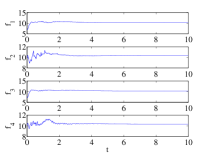
(g) Quadrotors total thrust inputs fisubscript๐‘“๐‘–f_{i}
Refer to caption
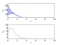
(h) Direction error eqsubscript๐‘’๐‘že_{q}, and angular velocity error eฯ‰subscript๐‘’๐œ”e_{\omega} for the links
Figure 3: Stabilization of a rigid-body connected to multiple quadrotors

The mass properties of quadrotors are chosen as

mi=0.755โ€‹kg,subscript๐‘š๐‘–0.755kg\displaystyle m_{i}=0.755\,\mathrm{kg},
Ji=diag[0.557,โ€„0.557,โ€„1.05]ร—10โˆ’2โ€‹kgm2.subscript๐ฝ๐‘–diag0.5570.5571.05superscript102superscriptkgm2\displaystyle J_{i}=\mathop{\mathrm{diag}}[0.557,\;0.557,\;1.05]\times 10^{-2}\mathrm{kgm^{2}}. (45)

The payload is a box with mass m0=0.5โ€‹kgsubscript๐‘š00.5kgm_{0}=0.5\,\mathrm{kg}, and its length, width, and height are 0.60.60.6, 0.80.80.8, and 0.2โ€‹m0.2m0.2\,\mathrm{m}, respectively. Each cable connecting the rigid body to the i๐‘–i-th quadrotor is considered to be ni=5subscript๐‘›๐‘–5n_{i}=5 rigid links. All the links have the same mass of miโ€‹j=0.01โ€‹kgsubscript๐‘š๐‘–๐‘—0.01kgm_{ij}=0.01\,\mathrm{kg} and length of liโ€‹j=0.15โ€‹msubscript๐‘™๐‘–๐‘—0.15ml_{ij}=0.15\,\mathrm{m}. Each cable is attached to the following points of the payload

ฯ1=[0.3,โˆ’0.4,โˆ’0.1]Tโ€‹m,ฯ2=[0.3,โ€„0.4,โˆ’0.1]Tโ€‹m,formulae-sequencesubscript๐œŒ1superscript0.30.40.1๐‘‡msubscript๐œŒ2superscript0.30.40.1๐‘‡m\displaystyle\rho_{1}=[0.3,\;-0.4,\;-0.1]^{T}\,\mathrm{m},\;\rho_{2}=[0.3,\;0.4,\;-0.1]^{T}\,\mathrm{m},
ฯ3=[โˆ’0.3,โˆ’0.4,โˆ’0.1]Tโ€‹m,ฯ4=[โˆ’0.3,โ€„0.4,โˆ’0.1]Tโ€‹m.formulae-sequencesubscript๐œŒ3superscript0.30.40.1๐‘‡msubscript๐œŒ4superscript0.30.40.1๐‘‡m\displaystyle\rho_{3}=[-0.3,\;-0.4,\;-0.1]^{T}\,\mathrm{m},\;\rho_{4}=[-0.3,\;0.4,\;-0.1]^{T}\,\mathrm{m}.

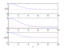
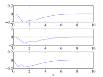
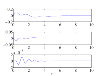
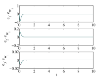
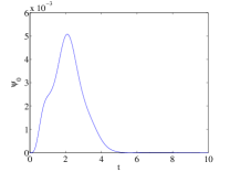
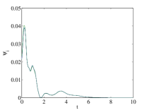
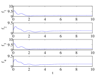
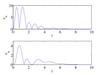
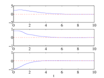
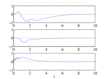
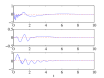
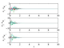
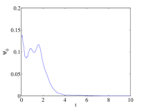
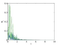
Numerical simulation results are presented at Figure 3, which shows the position and velocity of the payload, and its tracking errors. We have also presented the link direction and link angular velocity errors defined as

eq=โˆ‘i=1mโˆ‘j=1niโ€–qiโ€‹jโˆ’e3โ€–,subscript๐‘’๐‘žsuperscriptsubscript๐‘–1๐‘šsuperscriptsubscript๐‘—1subscript๐‘›๐‘–normsubscript๐‘ž๐‘–๐‘—subscript๐‘’3\displaystyle e_{q}=\sum_{i=1}^{m}\sum_{j=1}^{n_{i}}\|q_{ij}-e_{3}\|, (46)
eฯ‰=โˆ‘i=1mโˆ‘j=1niโ€–ฯ‰iโ€‹jโ€–.subscript๐‘’๐œ”superscriptsubscript๐‘–1๐‘šsuperscriptsubscript๐‘—1subscript๐‘›๐‘–normsubscript๐œ”๐‘–๐‘—\displaystyle e_{\omega}=\sum_{i=1}^{m}\sum_{j=1}^{n_{i}}\|\omega_{ij}\|. (47)

Refer to caption
(a) 3D perspective

Refer to caption
(b) Side view

Refer to caption
(c) Top view
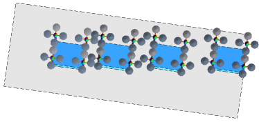
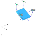
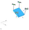
Figure 4: Snapshots of controlled maneuver

Refer to caption
(a) Payload position x0subscript๐‘ฅ0x_{0}:blue, x0dsubscript๐‘ฅsubscript0๐‘‘x_{0_{d}}:red
Refer to caption
(b) Payload velocity v0subscript๐‘ฃ0v_{0}:blue, v0dsubscript๐‘ฃsubscript0๐‘‘v_{0_{d}}:red

Refer to caption
(c) Payload angular velocity ฮฉ0subscriptฮฉ0\Omega_{0}
Refer to caption
(d) Quadrotors angular velocity errors eฮฉisubscript๐‘’subscriptฮฉ๐‘–e_{\Omega_{i}}

Refer to caption
(e) Payload attitude error ฯˆ0subscript๐œ“0\psi_{0}
Refer to caption
(f) Quadrotors attitude errors ฯˆisubscript๐œ“๐‘–\psi_{i}

Refer to caption
(g) Quadrotors total thrust inputs fisubscript๐‘“๐‘–f_{i}
Refer to caption
(h) Direction error eqsubscript๐‘’๐‘že_{q}, and angular velocity error eฯ‰subscript๐‘’๐œ”e_{\omega} for the links
Figure 5: Stabilization of a payload with multiple quadrotors connected with flexible cables.

5.2 Payload Stabilization with Large Initial Attitude Errors

In the second case, we consider large initial errors for the attitude of the payload and quadrotors. Initially, the rigid body is tilted about its b1subscript๐‘1b_{1} axis by 303030 degrees, and the initial direction of the links are chosen such that two cables are curved along the horizontal direction. The initial conditions are given by

x0โ€‹(0)=[2.4,โ€„0.8,โˆ’1.0]T,v0โ€‹(0)=03ร—1,formulae-sequencesubscript๐‘ฅ00superscript2.40.81.0๐‘‡subscript๐‘ฃ00subscript031\displaystyle x_{0}(0)=[2.4,\;0.8,\;-1.0]^{T},\;v_{0}(0)=0_{3\times 1},
ฯ‰iโ€‹jโ€‹(0)=03ร—1,ฮฉiโ€‹(0)=03ร—1formulae-sequencesubscript๐œ”๐‘–๐‘—0subscript031subscriptฮฉ๐‘–0subscript031\displaystyle\omega_{ij}(0)=0_{3\times 1},\;\Omega_{i}(0)=0_{3\times 1}
R0โ€‹(0)=Rxโ€‹(30โˆ˜),ฮฉ0=03ร—1,formulae-sequencesubscript๐‘…00subscript๐‘…๐‘ฅsuperscript30subscriptฮฉ0subscript031\displaystyle R_{0}(0)=R_{x}(30^{\circ}),\;\Omega_{0}=0_{3\times 1},

where Rxโ€‹(30โˆ˜)subscript๐‘…๐‘ฅsuperscript30R_{x}(30^{\circ}) denotes the rotation about the first axis by 30โˆ˜superscript3030^{\circ}. The initial attitude of quadrotors are chosen as

R1โ€‹(0)=Ryโ€‹(โˆ’35โˆ˜),R2โ€‹(0)=I3ร—3,formulae-sequencesubscript๐‘…10subscript๐‘…๐‘ฆsuperscript35subscript๐‘…20subscript๐ผ33\displaystyle R_{1}(0)=R_{y}(-35^{\circ}),\;R_{2}(0)=I_{3\times 3},
R3โ€‹(0)=Ryโ€‹(โˆ’35โˆ˜),R4โ€‹(0)=I3ร—3.formulae-sequencesubscript๐‘…30subscript๐‘…๐‘ฆsuperscript35subscript๐‘…40subscript๐ผ33\displaystyle R_{3}(0)=R_{y}(-35^{\circ}),\;R_{4}(0)=I_{3\times 3}.

The mass properties of quadrotors are chosen as pervious example. The payload is a box with mass m0=0.5โ€‹kgsubscript๐‘š00.5kgm_{0}=0.5\,\mathrm{kg}, and its length, width, and height are 0.60.60.6, 0.80.80.8, and 0.2โ€‹m0.2m0.2\,\mathrm{m}, respectively. Each cable connecting the rigid body to the i๐‘–i-th quadrotor is considered to be ni=5subscript๐‘›๐‘–5n_{i}=5 rigid links. All the links have the same mass of miโ€‹j=0.01โ€‹kgsubscript๐‘š๐‘–๐‘—0.01kgm_{ij}=0.01\,\mathrm{kg} and length of liโ€‹j=0.15โ€‹msubscript๐‘™๐‘–๐‘—0.15ml_{ij}=0.15\,\mathrm{m}. Each cable is attached to the following points of the payload

ฯ1=[0.3,โˆ’0.4,โˆ’0.1]Tโ€‹m,ฯ2=[0.3,โ€„0.4,โˆ’0.1]Tโ€‹m,formulae-sequencesubscript๐œŒ1superscript0.30.40.1๐‘‡msubscript๐œŒ2superscript0.30.40.1๐‘‡m\displaystyle\rho_{1}=[0.3,\;-0.4,\;-0.1]^{T}\,\mathrm{m},\;\rho_{2}=[0.3,\;0.4,\;-0.1]^{T}\,\mathrm{m},
ฯ3=[โˆ’0.3,โˆ’0.4,โˆ’0.1]Tโ€‹m,ฯ4=[โˆ’0.3,โ€„0.4,โˆ’0.1]Tโ€‹m.formulae-sequencesubscript๐œŒ3superscript0.30.40.1๐‘‡msubscript๐œŒ4superscript0.30.40.1๐‘‡m\displaystyle\rho_{3}=[-0.3,\;-0.4,\;-0.1]^{T}\,\mathrm{m},\;\rho_{4}=[-0.3,\;0.4,\;-0.1]^{T}\,\mathrm{m}.

The payload mass is m=1.0โ€‹kg๐‘š1.0kgm=1.0\,\mathrm{kg} , and its length, width, and height are 1.01.01.0, 1.21.21.2, and 0.2โ€‹m0.2m0.2\,\mathrm{m}, respectively.

Refer to caption
(a) t=0๐‘ก0t=0 Sec.
Refer to caption
(b) t=0.14๐‘ก0.14t=0.14 Sec.
Refer to caption
(c) t=0.30๐‘ก0.30t=0.30 Sec.

Refer to caption
(d) t=0.68๐‘ก0.68t=0.68 Sec.
Refer to caption
(e) t=1.10๐‘ก1.10t=1.10 Sec.
Refer to caption
(f) t=1.36๐‘ก1.36t=1.36 Sec.

Refer to caption
(g) t=1.98๐‘ก1.98t=1.98 Sec.
Refer to caption
(h) t=3.48๐‘ก3.48t=3.48 Sec.
Refer to caption
(i) t=10๐‘ก10t=10 Sec.
Figure 6: Snapshots of the controlled maneuver. A short animation is also available at https://www.youtube.com/watch?v=j14tSuHd8oA

Figure 5 illustrates the tracking errors, and the total thrust of each quadrotor. Snapshots of the controlled maneuvers is also illustrated at Figure 6. It is shown that the proposed controller is able to stabilize the payload and cables at their desired configuration even from the large initial attitude errors.

6 EXPERIMENT

In this section, an experimental setup is described and the proposed geometric nonlinear controller is validated with experiments.

6.1 Hardware Description

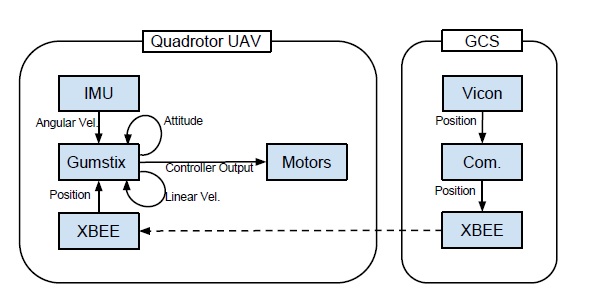
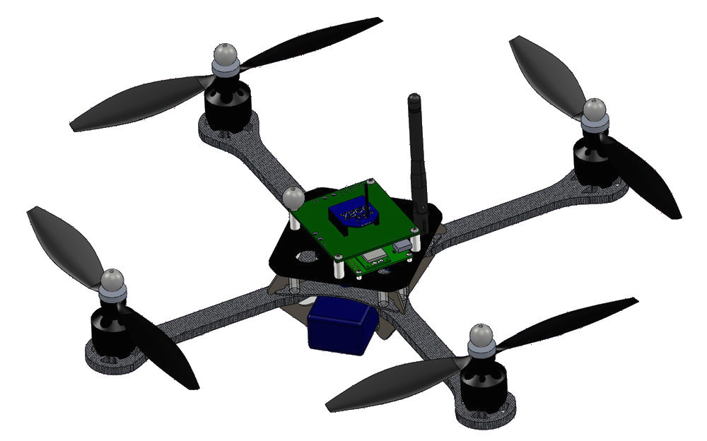
The quadrotor UAV developed at the flight dynamics and control laboratory at the George Washington University is shown at Figureย 7(a), and its parameters are the same as described as the previous section. The angular velocity is measured from inertial measurement unit (IMU) and the attitude is obtained from IMU data. Position of the UAV is measured from motion capture system (Vicon) and the velocity is estimated from the measurement. Ground computing system receives the Vicon data and send it to the UAV via XBee. The Gumstix is adopted as micro computing unit on the UAV. The flight control software has three main threads, namely Vicon thread, IMU thread, and control thread. The Vicon thread receives the Vicon measurement and estimates linear velocity of the quadrotor. In IMU thread, it receives the IMU measurement and estimates the attitude. The last thread handles the control outputs at each time step. Also, control outputs are calculated at 120Hz which is fast enough to run any kind of aggressive maneuvers. Information flow of the system is illustrated in Figure 9.

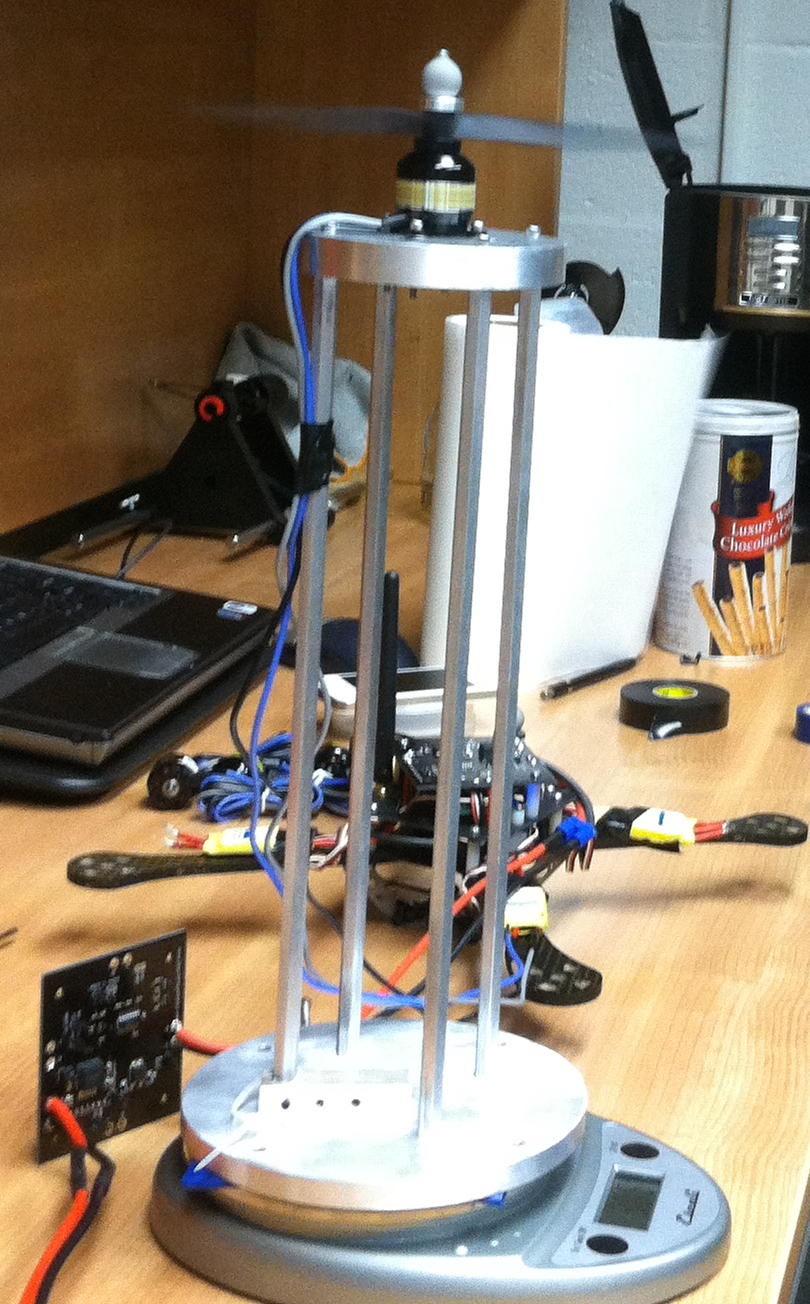
We developed an accurate CAD model as shown in Figureย 8 to identify several parameters of the quadrotor, such as moment of inertia and center of mass. Furthermore, a precise rotor calibration is performed for each rotor, with a custom-made thrust stand as shown in Figureย 7(b) to determine the relation between the command in the motor speed controller and the actual thrust. For various values of motor speed commands, the corresponding thrust is measured, and those data are fitted with a second order polynomial.
Refer to caption OMAP 600MHz Processor Attitude sensor 3DM-GX3 via UART BLDC Motor via I2C Safety Switch XBee RF WIFI to Ground Station LiPo Battery 11.1V, 2200mAh
(a) Hardware configuration
Refer to caption
(b) Motor calibration setup
Figure 7: Hardware development for each quadrotor UAV

Refer to caption

Figure 8: CAD Model

Refer to caption


Figure 9: Information flow of overall system

6.2 Stabilizing a Rod with Two Quadrotors

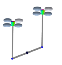
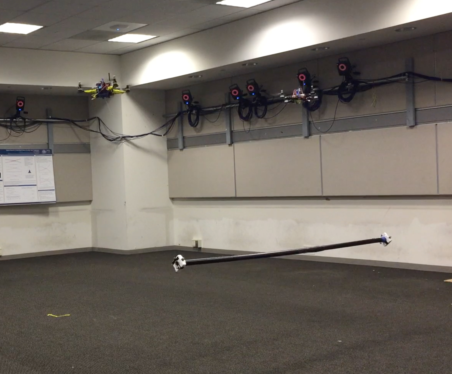
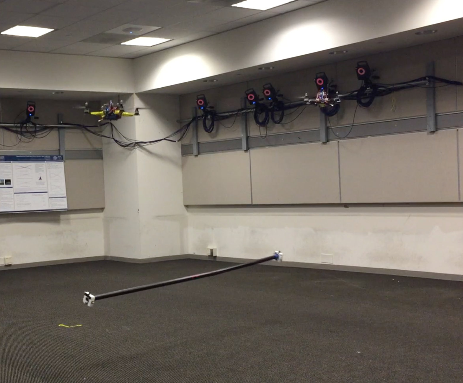
As a special case of rigid body payload, we considered a rod as a payload for experiment as shown in the Figuresย 10. Two quadrotors are enough for this experiment to control the position of the payload.

Refer to caption
(a) Experiment
Refer to caption

m1,J1,x1subscript๐‘š1subscript๐ฝ1subscript๐‘ฅ1m_{1},J_{1},x_{1} โ†“q1,l1โ†“absentsubscript๐‘ž1subscript๐‘™1\downarrow q_{1},l_{1} m0,x0,q0โ†’โ†’subscript๐‘š0subscript๐‘ฅ0subscript๐‘ž0absentm_{0},x_{0},q_{0}\rightarrow l0subscript๐‘™0l_{0} l0subscript๐‘™0l_{0} โ†“q2,l2โ†“absentsubscript๐‘ž2subscript๐‘™2\downarrow q_{2},l_{2} m2,J2,x2subscript๐‘š2subscript๐ฝ2subscript๐‘ฅ2m_{2},J_{2},x_{2}

(b) Simulation
Figure 10: Two quadrotors transporting a rod

We prepared a benchmark and a proposed controller case for this experiment. In both cases, two quadrotors are employed to hover at a fixed position initially while holding a rigid body rod which is at the equilibrium of the whole system. Then we utilized a wire to pull the payload and releasing it to simulate the disturbance. The performance of the proposed controller is then compared to the situation where there is no active controller specially works to stabilize the payload (benchmark). Both cables have length of l1,l2=1.3subscript๐‘™1subscript๐‘™21.3l_{1},l_{2}=1.3 m๐‘šm and rod has mass and length of m0=0.52subscript๐‘š00.52m_{0}=0.52 kโ€‹g๐‘˜๐‘”kg and 2โ€‹l0=2.052subscript๐‘™02.052l_{0}=2.05 m๐‘šm respectively. Each quadrotor has mass of m1=m2=0.755subscript๐‘š1subscript๐‘š20.755m_{1}=m_{2}=0.755 kโ€‹g๐‘˜๐‘”kg and the following moment of inertia which is obtained from the CAD model

J1,J2=[5.57110.0618โˆ’0.02510.061775.57570.0101โˆ’0.025020.010071.05053]ร—10โˆ’2kgm2.formulae-sequencesubscript๐ฝ1subscript๐ฝ2matrix5.57110.06180.02510.061775.57570.01010.025020.010071.05053superscript102superscriptkgm2\displaystyle J_{1},J_{2}=\begin{bmatrix}5.5711&0.0618&-0.0251\\ 0.06177&5.5757&0.0101\\ -0.02502&0.01007&1.05053\end{bmatrix}\times 10^{-2}\quad\mathrm{kgm}^{2}.

The following relations and initial conditions is applied for both cases for this equilibrium condition

q0โ€‹(0)=e1,q1โ€‹(0)=q2โ€‹(0)=e3,formulae-sequencesubscript๐‘ž00subscript๐‘’1subscript๐‘ž10subscript๐‘ž20subscript๐‘’3\displaystyle q_{0}(0)=e_{1},\quad q_{1}(0)=q_{2}(0)=e_{3},
x1โ€‹(0)=x0โ€‹(0)โˆ’l0โ€‹q0โ€‹(0)โˆ’l1โ€‹q1โ€‹(0),subscript๐‘ฅ10subscript๐‘ฅ00subscript๐‘™0subscript๐‘ž00subscript๐‘™1subscript๐‘ž10\displaystyle x_{1}(0)=x_{0}(0)-l_{0}q_{0}(0)-l_{1}q_{1}(0),
x2โ€‹(0)=x0โ€‹(0)+l0โ€‹q0โ€‹(0)โˆ’l1โ€‹q2โ€‹(0),subscript๐‘ฅ20subscript๐‘ฅ00subscript๐‘™0subscript๐‘ž00subscript๐‘™1subscript๐‘ž20\displaystyle x_{2}(0)=x_{0}(0)+l_{0}q_{0}(0)-l_{1}q_{2}(0),
R1=R2=I3,subscript๐‘…1subscript๐‘…2subscript๐ผ3\displaystyle R_{1}=R_{2}=I_{3},
ฮฉ1=ฮฉ2=ฮฉ0=0,subscriptฮฉ1subscriptฮฉ2subscriptฮฉ00\displaystyle\Omega_{1}=\Omega_{2}=\Omega_{0}=0,

6.2.1 Benchmark

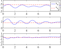
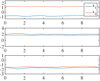
We choose this case as a comparison benchmark and itโ€™s not the result of the proposed controller in this paper. In this case, two quadrotors are hovering above the payload while cables are aligned to the vertical direction and we apply a disturbance to the payload. Here, the cables and payload dynamics are not considered into the control system and geometric nonlinear controller is used for each quadrotor to maintain quadrotors hovering at the fixed position and considers the forces applied to the quadrotors form the payload as disturbance. The payload is pulled by 30โˆ˜superscript3030^{\circ} in the direction of y๐‘ฆy-axis of inertial frame and releases. The payload is oscillating bellow the quadrotors and forces applies to each quadrotor from the cables are just considered as disturbances to the quadrotors, so we experience large oscillations of the payload and cables.
Refer to caption
(a) Rodโ€™s actual and desired positions, x0subscript๐‘ฅ0x_{0}, x0dsubscript๐‘ฅsubscript0๐‘‘x_{0_{d}}
Refer to caption
(b) Quadrotorโ€™s positions, x1subscript๐‘ฅ1x_{1}, x2subscript๐‘ฅ2x_{2}

Refer to caption
(c) First cableโ€™s direction, q1subscript๐‘ž1q_{1}
Refer to caption
(d) Second cableโ€™s direction, q2subscript๐‘ž2q_{2}
Figure 11: Benchmark: quadrotor position control systemย [23]

Numerical results for this experiment are presented in Figuresย 11 which presents the first and secondโ€™s link directions, position of the payload and positions of the quadrotors during this test.

6.2.2 Proposed Dynamical System and Controller

In this case, quadrotors are hovering at a fixed position using the geometric nonlinear controller while holding the payload. The payload is pulled with an external wire up to 30โˆ˜superscript3030^{\circ} angle same as the first case and then releases. Then, the proposed controller is switched in to stabilize the system. In this scenario, dynamic of the cables and payload are considered into the control system and quadrotors cooperatively work to stabilize the payload to the desired fixed position while aligning the cables in the vertical directions and the payload in the desired direction of first inertial axis, e1subscript๐‘’1e_{1}.

Refer to caption
(a) Rodโ€™s actual and desired positions, x0subscript๐‘ฅ0x_{0}, x0dsubscript๐‘ฅsubscript0๐‘‘x_{0_{d}}
Refer to caption
(b) Quadrotorโ€™s positions, x1subscript๐‘ฅ1x_{1}, x2subscript๐‘ฅ2x_{2}

Refer to caption
(c) First cableโ€™s direction, q1subscript๐‘ž1q_{1}
Refer to caption
(d) Second cableโ€™s direction, q2subscript๐‘ž2q_{2}
Figure 12: Proposed Controller: two quadrotors with rigid body payload. (The vertical dotted line indicates the time when controller switched in and stabilizes the system.)

Figureย 12 illustrates the position of the payload and quadrotors during this experiment where we applied the proposed controller. The vertical dotted line indicates the time when geometric nonlinear controller is switched with the proposed controller and stabilizes the system.

As shown in this figure, the proposed controller reduces and eliminates the oscillations of the cables and payload much effectively while considering the payload and cables dynamics. The desired cables directions are along the vertical direction e3=[0,โ€„0,โ€„1]Tsubscript๐‘’3superscript0โ€„01๐‘‡e_{3}=[0,\;0,\;1]^{T} and the desired rodโ€™s directions is along the e1subscript๐‘’1e_{1} axis.

Refer to caption
Refer to caption

Refer to caption
Refer to caption
Figure 13: Snapshots of controlled stabilization of a rod with two quadrotors. A short video of this comparison is available at https://www.youtube.com/watch?v=u65GqIl2skY

Snapshots of the controlled maneuvers is also illustrated at Figure 13.

7 Conclusions

We utilized Euler-Lagrange equations to derive the complete model of multiple quadrotor UAVs transporting a rigid-body connected via flexible cables in 3D space. These derivations are developed in a remarkably compact form which allow us to choose an arbitrary number and any configuration of the links and an arbitrary number of quadrotors. We developed a geometric nonlinear controller to stabilize the links below the quadrotors and payload in the equilibrium position from an initial condition. We expanded these derivations in such a way that there is no need of using local angle coordinates which is an advantageous technique to signalize our derivations. A rigorous Lyapunov stability analysis is also presented to illustrate the stability properties without any time-scale separation. Numerical simulation and experimental results and for multiple cooperative quadrotors stabilizing a rigid-body performed and presented in this paper and shows the the accuracy and performance of the purposed model and control system.

{acknowledgment}

This research has been supported in part by NSF under the grant CMMI-1243000 (transferred from 1029551), CMMI-1335008, and CNS-1337722.

References

  • [1] Mellinger, D., Shomin, M., Michael, N., and Kumar, V., 2013. โ€œCooperative grasping and transport using multiple quadrotorsโ€. In Distributed Autonomous Robotic Systems, Vol.ย 83. Springer Berlin Heidelberg, pp.ย 545โ€“558.
  • [2] Kim, S., Choi, S., and Kim, H.ย J., 2013. โ€œAerial manipulation using a quadrotor with a two dof robotic armโ€. In Intelligent Robots and Systems, pp.ย 4990โ€“4995.
  • [3] Cicolani, L., Kanning, G., and Synnestvedt, R., 1995. โ€œSimulation of the dynamics of helicopter slung load systemsโ€. Journal of the American Helicopter Society, 40(4), pp.ย 44โ€“61.
  • [4] Bernard, M., 2009. โ€œGeneric slung load transportation system using small size helicoptersโ€. In Proceedings of the International Conference on Robotics and Automation, pp.ย 3258โ€“3264.
  • [5] Palunko, I., Cruz, P., and Fierro, R., 2012. โ€œAgile load transportationโ€. IEEE Robotics and Automation Magazine, 19(3), pp.ย 69โ€“79.
  • [6] Michael, N., Fink, J., and Kumar, V., 2011. โ€œCooperative manipulation and transportation with aerial robotsโ€. Autonomous Robots, 30, pp.ย 73โ€“86.
  • [7] Maza, I., Kondak, K., Bernard, M., and Ollero, A., 2010. โ€œMulti-UAV cooperation and control for load transportation and deploymentโ€. Journal of Intelligent and Robotic Systems, 57, pp.ย 417โ€“449.
  • [8] Zameroski, D., Starr, G., Wood, J., and Lumia, R., 2008. โ€œRapid swing-free transport of nonlinear payloads using dynamic programmingโ€. Journal of Dynamic Systems, Measurement, and Control, 130(4), June, p.ย 041001.
  • [9] Schultz, J., and Murphey, T., 2012. โ€œTrajectory generation for underactuated control of a suspended massโ€. In IEEE International Conference on Robotics and Automation, pp.ย 123โ€“129.
  • [10] Palunko, I., Fierro, R., and Cruz, P., 2012. โ€œTrajectory generation for swing-free maneuvers of a quadrotor with suspended payload: A dynamic programming approachโ€. In IEEE International Conference on Robotics and Automation.
  • [11] Lee, T., Sreenath, K., and Kumar, V., 2013. โ€œGeometric control of cooperating multiple quadrotor UAVs with a suspended loadโ€. In Proceedings of the IEEE Conference on Decision and Control, Vol.ย 5510โ€“5515.
  • [12] Goodarzi, F.ย A., Lee, D., and Lee, T., 2014. โ€œGeometric stabilization of quadrotor UAV with a payload connected by flexible cableโ€. In Proceedings of American Control Conference, Portland OR, pp.ย 4925โ€“4930.
  • [13] Goodarzi, F.ย A., Lee, D., and Lee, T., 2015. โ€œGeometric control of a quadrotor uav transporting a payload connected via flexible cableโ€. International Journal of Control, Automation and Systems, 13(6).
  • [14] Lee, T., 2014. โ€œDynamics and control of quadrotor uavs transporting a rigid body connected via flexible cablesโ€. In Proceedings of 53rd IEEE Conference on Decision and Control, pp.ย 6155โ€“6160.
  • [15] Mellinger, D., Michael, N., and Kumar, V., 2012. โ€œTrajectory generation and control for precise aggressive maneuvers with quadrotorsโ€. International Journal Of Robotics Research, 31(5), pp.ย 664โ€“674.
  • [16] Tayebi, A., and McGilvray, S., 2006. โ€œAttitude stabilization of a VTOL quadrotor aircraftโ€. IEEE Transactions on Control System Technology, 14(3), pp.ย 562โ€“571.
  • [17] Bhat, S., and Bernstein, D., 2000. โ€œA topological obstruction to continuous global stabilization of rotational motion and the unwinding phenomenonโ€. Systems and Control Letters, 39(1), pp.ย 66โ€“73.
  • [18] Mayhew, C., Sanfelice, R., and Teel, A., 2011. โ€œQuaternion-based hybrid control for robust global attitude trackingโ€. IEEE Transactions on Automatic Control.
  • [19] Goodarzi, F.ย A., Lee, D., and Lee, T., 2015. โ€œGeometric adaptive tracking control of a quadrotor unmanned aerial vehicle on ๐–ฒ๐–คโ€‹(๐Ÿฅ)๐–ฒ๐–ค3\mathsf{SE(3)} for agile maneuversโ€. Journal of Dynamic Systems, Measurement, and Control, 137(9), September, pp.ย 091007โ€“12.
  • [20] Izadi, M., Bohn, J., Lee, D., Sanyal, A., Butcher, E., and Scheeres, D., 2013. โ€œA nonlinear observer design for a rigid body in the proximity of a spherical asteroidโ€. In Proceedings of the ASME Dynamic Systems and Control Conference, Palo Alto, CA, USA.
  • [21] Izadi, M., Sanyal, A., Barany, E., and Viswanathan, S., 2015. โ€œRigid body motion estimation based on the Lagrangeโ€“dโ€™Alembert principleโ€. In Proceedings of the 54nโ€‹dsuperscript54๐‘›๐‘‘54^{nd} IEEE Conference on Decision and Control.
  • [22] Lee, T., Leok, M., and McClamroch, N., 2012. โ€œNonlinear robust tracking control of a quadrotor UAV on ๐–ฒ๐–คโ€‹(๐Ÿฅ)๐–ฒ๐–ค3\mathsf{SE(3)}โ€. In Proceeding of the American Control Conference, pp.ย 4649โ€“4654.
  • [23] Goodarzi, F., Lee, D., and Lee, T., 2013. โ€œGeometric nonlinear PID control of a quadrotor UAV on ๐–ฒ๐–คโ€‹(๐Ÿฅ)๐–ฒ๐–ค3\mathsf{SE(3)}โ€. In in Proceedings of the European Control Conference, pp.ย 3845โ€“3850.
  • [24] Chaturvedi, N., Sanyal, A., and McClamroch, N., 2011. โ€œRigid-body attitude controlโ€. IEEE Control Systems Magazine, 31(3), pp.ย 30โ€“51.
  • [25] Izadi, M., Sanyal, A., Beard, R., and Bai, H., 2015. โ€œGPS-denied relative motion estimation for fixed-wing UAV using the variational pose estimatorโ€. In Proceedings of the 54nโ€‹dsuperscript54๐‘›๐‘‘54^{nd} IEEE Conference on Decision and Control.
  • [26] Goodarzi, F.ย A., and Lee, T., 2015. โ€œDynamics and control of quadrotor UAVs transporting a rigid body connected via flexible cablesโ€. In Proceedings of American Control Conference 2015, Chicago IL, pp.ย 4677โ€“4682.
  • [27] T.ย Lee, M.ย L., and McClamroch, N., 2013. โ€œNonlinear robust tracking control of a quadrotor UAV on ๐–ฒ๐–คโ€‹(๐Ÿฅ)๐–ฒ๐–ค3\mathsf{SE(3)}โ€. Asian Journal of Control, 15(2), Mar., pp.ย 391โ€“408.
  • [28] Goodarzi, F.ย A., 2015. โ€œGeometric nonlinear controls for multiple cooperative quadrotor UAVs transporting a rigid bodyโ€. PhD thesis, The George Washington University, August.
  • [29] Lee, T., 2008. โ€œComputational geometric mechanics and control of rigid bodiesโ€. PhD thesis, University of Michigan.
  • [30] Lee, T., Leok, M., and McClamroch, N.ย H., 2009. โ€œLagrangian mechanics and variational integrators on two-spheresโ€. International Journal for Numerical Methods in Engineering, 79(9), pp.ย 1147โ€“1174.
  • [31] Khalil, H., 1996. Nonlinear Systems. Prentice Hall, 2nd Edition.
  • [32] Fernando, T., Chandiramani, J., Lee, T., and Gutierrez, H., 2011. โ€œRobust adaptive geometric tracking controls on SO(3) with an application to the attitude dynamics of a quadrotor uavโ€. In Proceedings of the IEEE Conference on Decision and Control, pp.ย 7380โ€“7385.

Appendix A Proof for Proposition 1

A.1 Kinetic Energy

The kinetic energy of the whole system is composed of the kinetic energy of quadrotors, cables and the rigid body, as

T=๐‘‡absent\displaystyle T= 12โ€‹m0โ€‹โ€–xห™0โ€–2+โˆ‘i=1nโˆ‘j=1ni12โ€‹miโ€‹jโ€‹โ€–xห™iโ€‹jโ€–2+12โ€‹โˆ‘i=1nmiโ€‹โ€–xห™iโ€–212subscript๐‘š0superscriptnormsubscriptห™๐‘ฅ02superscriptsubscript๐‘–1๐‘›superscriptsubscript๐‘—1subscript๐‘›๐‘–12subscript๐‘š๐‘–๐‘—superscriptnormsubscriptห™๐‘ฅ๐‘–๐‘—212superscriptsubscript๐‘–1๐‘›subscript๐‘š๐‘–superscriptnormsubscriptห™๐‘ฅ๐‘–2\displaystyle\frac{1}{2}m_{0}\|\dot{x}_{0}\|^{2}+\sum_{i=1}^{n}\sum_{j=1}^{n_{i}}{\frac{1}{2}m_{ij}\|\dot{x}_{ij}\|^{2}}+\frac{1}{2}\sum_{i=1}^{n}{m_{i}\|\dot{x}_{i}\|^{2}}
+12โ€‹โˆ‘i=1nฮฉiโ‹…Jiโ€‹ฮฉi+12โ€‹ฮฉ0โ‹…J0โ€‹ฮฉ0.12superscriptsubscript๐‘–1๐‘›โ‹…subscriptฮฉ๐‘–subscript๐ฝ๐‘–subscriptฮฉ๐‘–โ‹…12subscriptฮฉ0subscript๐ฝ0subscriptฮฉ0\displaystyle+\frac{1}{2}\sum_{i=1}^{n}{\Omega_{i}\cdot J_{i}\Omega_{i}}+\frac{1}{2}\Omega_{0}\cdot J_{0}\Omega_{0}. (48)

Substituting the derivatives of (6) and (7) into the above expression we have

T=๐‘‡absent\displaystyle T= 12โ€‹m0โ€‹โ€–xห™0โ€–2+โˆ‘i=1nโˆ‘j=1ni12โ€‹miโ€‹jโ€‹โ€–xห™0+Rห™0โ€‹ฯiโˆ’โˆ‘a=j+1niliโ€‹aโ€‹qห™iโ€‹aโ€–212subscript๐‘š0superscriptnormsubscriptห™๐‘ฅ02superscriptsubscript๐‘–1๐‘›superscriptsubscript๐‘—1subscript๐‘›๐‘–12subscript๐‘š๐‘–๐‘—superscriptnormsubscriptห™๐‘ฅ0subscriptห™๐‘…0subscript๐œŒ๐‘–superscriptsubscript๐‘Ž๐‘—1subscript๐‘›๐‘–subscript๐‘™๐‘–๐‘Žsubscriptห™๐‘ž๐‘–๐‘Ž2\displaystyle\frac{1}{2}m_{0}\|\dot{x}_{0}\|^{2}+\sum_{i=1}^{n}\sum_{j=1}^{n_{i}}{\frac{1}{2}m_{ij}\|\dot{x}_{0}+\dot{R}_{0}\rho_{i}-\sum_{a=j+1}^{n_{i}}{l_{ia}\dot{q}_{ia}}\|^{2}}
+12โ€‹โˆ‘i=1nmiโ€‹โ€–xห™0+Rห™0โ€‹ฯiโˆ’โˆ‘a=1niliโ€‹aโ€‹qห™iโ€‹aโ€–212superscriptsubscript๐‘–1๐‘›subscript๐‘š๐‘–superscriptnormsubscriptห™๐‘ฅ0subscriptห™๐‘…0subscript๐œŒ๐‘–superscriptsubscript๐‘Ž1subscript๐‘›๐‘–subscript๐‘™๐‘–๐‘Žsubscriptห™๐‘ž๐‘–๐‘Ž2\displaystyle+\frac{1}{2}\sum_{i=1}^{n}{m_{i}\|\dot{x}_{0}+\dot{R}_{0}\rho_{i}-\sum_{a=1}^{n_{i}}{l_{ia}\dot{q}_{ia}}\|^{2}}
+12โ€‹โˆ‘i=1nฮฉiโ‹…Jiโ€‹ฮฉi+12โ€‹ฮฉ0โ‹…J0โ€‹ฮฉ0.12superscriptsubscript๐‘–1๐‘›โ‹…subscriptฮฉ๐‘–subscript๐ฝ๐‘–subscriptฮฉ๐‘–โ‹…12subscriptฮฉ0subscript๐ฝ0subscriptฮฉ0\displaystyle+\frac{1}{2}\sum_{i=1}^{n}{\Omega_{i}\cdot J_{i}\Omega_{i}}+\frac{1}{2}\Omega_{0}\cdot J_{0}\Omega_{0}. (49)

We expand the above expression as follow

T=๐‘‡absent\displaystyle T= 12โ€‹(m0โ€‹โ€–xห™0โ€–2+โˆ‘i=1nโˆ‘j=1nimiโ€‹jโ€‹โ€–xห™0โ€–2+โˆ‘i=1nmiโ€‹โ€–xห™0โ€–2)12subscript๐‘š0superscriptnormsubscriptห™๐‘ฅ02superscriptsubscript๐‘–1๐‘›superscriptsubscript๐‘—1subscript๐‘›๐‘–subscript๐‘š๐‘–๐‘—superscriptnormsubscriptห™๐‘ฅ02superscriptsubscript๐‘–1๐‘›subscript๐‘š๐‘–superscriptnormsubscriptห™๐‘ฅ02\displaystyle\frac{1}{2}(m_{0}\|\dot{x}_{0}\|^{2}+\sum_{i=1}^{n}\sum_{j=1}^{n_{i}}{m_{ij}\|\dot{x}_{0}\|^{2}}+\sum_{i=1}^{n}{m_{i}\|\dot{x}_{0}\|^{2}})
+12โ€‹โˆ‘i=1n(โˆ‘j=1nimiโ€‹jโ€‹โ€–Rห™0โ€‹ฯiโ€–2+miโ€‹โ€–Rห™0โ€‹ฯiโ€–2)12superscriptsubscript๐‘–1๐‘›superscriptsubscript๐‘—1subscript๐‘›๐‘–subscript๐‘š๐‘–๐‘—superscriptnormsubscriptห™๐‘…0subscript๐œŒ๐‘–2subscript๐‘š๐‘–superscriptnormsubscriptห™๐‘…0subscript๐œŒ๐‘–2\displaystyle+\frac{1}{2}\sum_{i=1}^{n}(\sum_{j=1}^{n_{i}}{m_{ij}\|\dot{R}_{0}\rho_{i}\|^{2}}+m_{i}\|\dot{R}_{0}\rho_{i}\|^{2})
+โˆ‘i=1n(โˆ‘j=1nimiโ€‹jโ€‹xห™0โ‹…Rห™0โ€‹ฯi+miโ€‹xห™0โ‹…Rห™0โ€‹ฯi)superscriptsubscript๐‘–1๐‘›superscriptsubscript๐‘—1subscript๐‘›๐‘–โ‹…subscript๐‘š๐‘–๐‘—subscriptห™๐‘ฅ0subscriptห™๐‘…0subscript๐œŒ๐‘–โ‹…subscript๐‘š๐‘–subscriptห™๐‘ฅ0subscriptห™๐‘…0subscript๐œŒ๐‘–\displaystyle+\sum_{i=1}^{n}(\sum_{j=1}^{n_{i}}{m_{ij}\dot{x}_{0}\cdot\dot{R}_{0}\rho_{i}}+m_{i}\dot{x}_{0}\cdot\dot{R}_{0}\rho_{i})
+12โ€‹โˆ‘i=1n(โˆ‘j=1nimiโ€‹jโ€‹โ€–โˆ‘a=j+1niliโ€‹aโ€‹qห™iโ€‹aโ€–2+miโ€‹โ€–โˆ‘a=1niliโ€‹aโ€‹qห™iโ€‹aโ€–2)12superscriptsubscript๐‘–1๐‘›superscriptsubscript๐‘—1subscript๐‘›๐‘–subscript๐‘š๐‘–๐‘—superscriptnormsuperscriptsubscript๐‘Ž๐‘—1subscript๐‘›๐‘–subscript๐‘™๐‘–๐‘Žsubscriptห™๐‘ž๐‘–๐‘Ž2subscript๐‘š๐‘–superscriptnormsuperscriptsubscript๐‘Ž1subscript๐‘›๐‘–subscript๐‘™๐‘–๐‘Žsubscriptห™๐‘ž๐‘–๐‘Ž2\displaystyle+\frac{1}{2}\sum_{i=1}^{n}(\sum_{j=1}^{n_{i}}{m_{ij}\|\sum_{a=j+1}^{n_{i}}{l_{ia}\dot{q}_{ia}}\|^{2}}+{m_{i}\|\sum_{a=1}^{n_{i}}{l_{ia}\dot{q}_{ia}}\|^{2}})
โˆ’โˆ‘i=1n(โˆ‘j=1nimiโ€‹jโ€‹xห™0โ‹…โˆ‘a=j+1niliโ€‹aโ€‹qห™iโ€‹a+xห™0โ‹…โˆ‘a=1niliโ€‹aโ€‹qห™iโ€‹a)superscriptsubscript๐‘–1๐‘›superscriptsubscript๐‘—1subscript๐‘›๐‘–โ‹…subscript๐‘š๐‘–๐‘—subscriptห™๐‘ฅ0superscriptsubscript๐‘Ž๐‘—1subscript๐‘›๐‘–subscript๐‘™๐‘–๐‘Žsubscriptห™๐‘ž๐‘–๐‘Žโ‹…subscriptห™๐‘ฅ0superscriptsubscript๐‘Ž1subscript๐‘›๐‘–subscript๐‘™๐‘–๐‘Žsubscriptห™๐‘ž๐‘–๐‘Ž\displaystyle-\sum_{i=1}^{n}(\sum_{j=1}^{n_{i}}{m_{ij}\dot{x}_{0}}\cdot\sum_{a=j+1}^{n_{i}}{{l_{ia}\dot{q}_{ia}}}+\dot{x}_{0}\cdot\sum_{a=1}^{n_{i}}{l_{ia}\dot{q}_{ia}})
โˆ’โˆ‘i=1n(โˆ‘j=1nimiโ€‹jโ€‹Rห™0โ€‹ฯiโ‹…โˆ‘a=j+1niliโ€‹aโ€‹qห™iโ€‹a+miโ€‹Rห™0โ€‹ฯiโ‹…โˆ‘a=1niliโ€‹aโ€‹qห™iโ€‹a)superscriptsubscript๐‘–1๐‘›superscriptsubscript๐‘—1subscript๐‘›๐‘–โ‹…subscript๐‘š๐‘–๐‘—subscriptห™๐‘…0subscript๐œŒ๐‘–superscriptsubscript๐‘Ž๐‘—1subscript๐‘›๐‘–subscript๐‘™๐‘–๐‘Žsubscriptห™๐‘ž๐‘–๐‘Žโ‹…subscript๐‘š๐‘–subscriptห™๐‘…0subscript๐œŒ๐‘–superscriptsubscript๐‘Ž1subscript๐‘›๐‘–subscript๐‘™๐‘–๐‘Žsubscriptห™๐‘ž๐‘–๐‘Ž\displaystyle-\sum_{i=1}^{n}(\sum_{j=1}^{n_{i}}{m_{ij}\dot{R}_{0}\rho_{i}}\cdot\sum_{a=j+1}^{n_{i}}{l_{ia}\dot{q}_{ia}}+m_{i}\dot{R}_{0}\rho_{i}\cdot\sum_{a=1}^{n_{i}}{l_{ia}\dot{q}_{ia}})
+12โ€‹โˆ‘i=1nฮฉiโ‹…Jiโ€‹ฮฉi+12โ€‹ฮฉ0โ‹…J0โ€‹ฮฉ0,12superscriptsubscript๐‘–1๐‘›โ‹…subscriptฮฉ๐‘–subscript๐ฝ๐‘–subscriptฮฉ๐‘–โ‹…12subscriptฮฉ0subscript๐ฝ0subscriptฮฉ0\displaystyle+\frac{1}{2}\sum_{i=1}^{n}{\Omega_{i}\cdot J_{i}\Omega_{i}}+\frac{1}{2}\Omega_{0}\cdot J_{0}\Omega_{0}, (50)

and substituting (16), (17), it is rewritten as

T=๐‘‡absent\displaystyle T= 12โ€‹MTโ€‹โ€–xห™0โ€–2+12โ€‹โˆ‘i=1nMiโ€‹Tโ€‹โ€–Rห™0โ€‹ฯiโ€–2+โˆ‘i=1n(Miโ€‹Tโ€‹xห™0โ‹…Rห™0โ€‹ฯi)12subscript๐‘€๐‘‡superscriptnormsubscriptห™๐‘ฅ0212superscriptsubscript๐‘–1๐‘›subscript๐‘€๐‘–๐‘‡superscriptnormsubscriptห™๐‘…0subscript๐œŒ๐‘–2superscriptsubscript๐‘–1๐‘›โ‹…subscript๐‘€๐‘–๐‘‡subscriptห™๐‘ฅ0subscriptห™๐‘…0subscript๐œŒ๐‘–\displaystyle\frac{1}{2}M_{T}\|\dot{x}_{0}\|^{2}+\frac{1}{2}\sum_{i=1}^{n}{M_{iT}\|\dot{R}_{0}\rho_{i}\|^{2}}+\sum_{i=1}^{n}({M_{iT}\dot{x}_{0}\cdot\dot{R}_{0}\rho_{i}})
+โˆ‘i=1nโˆ‘j,k=1niM0โ€‹iโ€‹jโ€‹liโ€‹kโ€‹qห™iโ€‹jโ‹…qห™iโ€‹kโˆ’โˆ‘i=1n(xห™0โ‹…โˆ‘j=1niM0โ€‹iโ€‹jโ€‹liโ€‹jโ€‹qห™iโ€‹j)superscriptsubscript๐‘–1๐‘›superscriptsubscript๐‘—๐‘˜1subscript๐‘›๐‘–โ‹…subscript๐‘€0๐‘–๐‘—subscript๐‘™๐‘–๐‘˜subscriptห™๐‘ž๐‘–๐‘—subscriptห™๐‘ž๐‘–๐‘˜superscriptsubscript๐‘–1๐‘›โ‹…subscriptห™๐‘ฅ0superscriptsubscript๐‘—1subscript๐‘›๐‘–subscript๐‘€0๐‘–๐‘—subscript๐‘™๐‘–๐‘—subscriptห™๐‘ž๐‘–๐‘—\displaystyle+\sum_{i=1}^{n}\sum_{j,k=1}^{n_{i}}{M_{0ij}l_{ik}\dot{q}_{ij}\cdot\dot{q}_{ik}}-\sum_{i=1}^{n}({\dot{x}_{0}\cdot\sum_{j=1}^{n_{i}}{M_{0ij}l_{ij}\dot{q}_{ij}}})
โˆ’โˆ‘i=1n(Rห™0โ€‹ฯiโ‹…โˆ‘j=1niM0โ€‹iโ€‹jโ€‹liโ€‹jโ€‹qห™iโ€‹j)superscriptsubscript๐‘–1๐‘›โ‹…subscriptห™๐‘…0subscript๐œŒ๐‘–superscriptsubscript๐‘—1subscript๐‘›๐‘–subscript๐‘€0๐‘–๐‘—subscript๐‘™๐‘–๐‘—subscriptห™๐‘ž๐‘–๐‘—\displaystyle-\sum_{i=1}^{n}({\dot{R}_{0}\rho_{i}}\cdot\sum_{j=1}^{n_{i}}{M_{0ij}l_{ij}\dot{q}_{ij}})
+12โ€‹โˆ‘i=1nฮฉiโ‹…Jiโ€‹ฮฉi+12โ€‹ฮฉ0โ‹…J0โ€‹ฮฉ0.12superscriptsubscript๐‘–1๐‘›โ‹…subscriptฮฉ๐‘–subscript๐ฝ๐‘–subscriptฮฉ๐‘–โ‹…12subscriptฮฉ0subscript๐ฝ0subscriptฮฉ0\displaystyle+\frac{1}{2}\sum_{i=1}^{n}{\Omega_{i}\cdot J_{i}\Omega_{i}}+\frac{1}{2}\Omega_{0}\cdot J_{0}\Omega_{0}. (51)

A.2 Potential Energy

We can derive the potential energy expression by considering the gravitational forces on each part of system as given

V=โˆ’m0โ€‹gโ€‹e3โ‹…x0โˆ’โˆ‘i=1nmiโ€‹gโ€‹e3โ‹…xiโˆ’โˆ‘i=1nโˆ‘j=1nimiโ€‹jโ€‹gโ€‹e3โ‹…xiโ€‹j.๐‘‰โ‹…subscript๐‘š0๐‘”subscript๐‘’3subscript๐‘ฅ0superscriptsubscript๐‘–1๐‘›โ‹…subscript๐‘š๐‘–๐‘”subscript๐‘’3subscript๐‘ฅ๐‘–superscriptsubscript๐‘–1๐‘›superscriptsubscript๐‘—1subscript๐‘›๐‘–โ‹…subscript๐‘š๐‘–๐‘—๐‘”subscript๐‘’3subscript๐‘ฅ๐‘–๐‘—\displaystyle V=-m_{0}ge_{3}\cdot x_{0}-\sum_{i=1}^{n}{m_{i}ge_{3}}\cdot x_{i}-\sum_{i=1}^{n}\sum_{j=1}^{n_{i}}{m_{ij}ge_{3}}\cdot x_{ij}. (52)

Using (6) and (7), we obtain

V=๐‘‰absent\displaystyle V= โˆ’m0โ€‹gโ€‹e3โ‹…x0โˆ’โˆ‘i=1nmiโ€‹gโ€‹e3โ‹…(x0+R0โ€‹ฯiโˆ’โˆ‘a=1niliโ€‹aโ€‹qiโ€‹a)โ‹…subscript๐‘š0๐‘”subscript๐‘’3subscript๐‘ฅ0superscriptsubscript๐‘–1๐‘›โ‹…subscript๐‘š๐‘–๐‘”subscript๐‘’3subscript๐‘ฅ0subscript๐‘…0subscript๐œŒ๐‘–superscriptsubscript๐‘Ž1subscript๐‘›๐‘–subscript๐‘™๐‘–๐‘Žsubscript๐‘ž๐‘–๐‘Ž\displaystyle-m_{0}ge_{3}\cdot x_{0}-\sum_{i=1}^{n}{m_{i}ge_{3}}\cdot(x_{0}+R_{0}\rho_{i}-\sum_{a=1}^{n_{i}}{l_{ia}q_{ia}})
โˆ’โˆ‘i=1nโˆ‘j=1nimiโ€‹jโ€‹gโ€‹e3โ‹…(x0+R0โ€‹ฯiโˆ’โˆ‘a=j+1niliโ€‹aโ€‹qiโ€‹a),superscriptsubscript๐‘–1๐‘›superscriptsubscript๐‘—1subscript๐‘›๐‘–โ‹…subscript๐‘š๐‘–๐‘—๐‘”subscript๐‘’3subscript๐‘ฅ0subscript๐‘…0subscript๐œŒ๐‘–superscriptsubscript๐‘Ž๐‘—1subscript๐‘›๐‘–subscript๐‘™๐‘–๐‘Žsubscript๐‘ž๐‘–๐‘Ž\displaystyle-\sum_{i=1}^{n}\sum_{j=1}^{n_{i}}{m_{ij}ge_{3}}\cdot(x_{0}+R_{0}\rho_{i}-\sum_{a=j+1}^{n_{i}}{l_{ia}q_{ia}}), (53)

and utilizing (17), we can simplify the potential energy as

V=โˆ’MTโ€‹gโ€‹e3โ‹…x0โˆ’โˆ‘i=1nMiโ€‹Tโ€‹gโ€‹e3โ‹…R0โ€‹ฯi+โˆ‘i=1nโˆ‘j=1niM0โ€‹iโ€‹jโ€‹liโ€‹jโ€‹qiโ€‹jโ‹…e3.๐‘‰โ‹…subscript๐‘€๐‘‡๐‘”subscript๐‘’3subscript๐‘ฅ0superscriptsubscript๐‘–1๐‘›โ‹…subscript๐‘€๐‘–๐‘‡๐‘”subscript๐‘’3subscript๐‘…0subscript๐œŒ๐‘–superscriptsubscript๐‘–1๐‘›superscriptsubscript๐‘—1subscript๐‘›๐‘–โ‹…subscript๐‘€0๐‘–๐‘—subscript๐‘™๐‘–๐‘—subscript๐‘ž๐‘–๐‘—subscript๐‘’3\displaystyle V=-M_{T}ge_{3}\cdot x_{0}-\sum_{i=1}^{n}{M_{iT}ge_{3}\cdot R_{0}\rho_{i}}+\sum_{i=1}^{n}\sum_{j=1}^{n_{i}}{M_{0ij}l_{ij}q_{ij}\cdot e_{3}}. (54)

A.3 Derivatives of Lagrangian

We develop the equation of motion for the Lagrangian L=Tโˆ’V๐ฟ๐‘‡๐‘‰L=T-V. The derivatives of the Lagrangian are given by

Dxห™0โ€‹L=MTโ€‹xห™0+โˆ‘i=1nMiโ€‹Tโ€‹Rห™0โ€‹ฯiโˆ’โˆ‘i=1nโˆ‘j=1niM0โ€‹iโ€‹jโ€‹liโ€‹jโ€‹qห™iโ€‹j,subscript๐ทsubscriptห™๐‘ฅ0๐ฟsubscript๐‘€๐‘‡subscriptห™๐‘ฅ0superscriptsubscript๐‘–1๐‘›subscript๐‘€๐‘–๐‘‡subscriptห™๐‘…0subscript๐œŒ๐‘–superscriptsubscript๐‘–1๐‘›superscriptsubscript๐‘—1subscript๐‘›๐‘–subscript๐‘€0๐‘–๐‘—subscript๐‘™๐‘–๐‘—subscriptห™๐‘ž๐‘–๐‘—\displaystyle D_{\dot{x}_{0}}L=M_{T}\dot{x}_{0}+\sum_{i=1}^{n}{M_{iT}\dot{R}_{0}\rho_{i}}-\sum_{i=1}^{n}\sum_{j=1}^{n_{i}}{M_{0ij}l_{ij}\dot{q}_{ij}}, (55)
Dx0โ€‹L=MTโ€‹gโ€‹e3,subscript๐ทsubscript๐‘ฅ0๐ฟsubscript๐‘€๐‘‡๐‘”subscript๐‘’3\displaystyle D_{x_{0}}L=M_{T}ge_{3}, (56)
Dqห™iโ€‹jโ€‹L=โˆ‘i=1nโˆ‘j=1niM0โ€‹iโ€‹jโ€‹liโ€‹kโ€‹qห™iโ€‹kโˆ’โˆ‘i=1nM0โ€‹iโ€‹jโ€‹liโ€‹jโ€‹(xห™0+Rห™0โ€‹ฯi),subscript๐ทsubscriptห™๐‘ž๐‘–๐‘—๐ฟsuperscriptsubscript๐‘–1๐‘›superscriptsubscript๐‘—1subscript๐‘›๐‘–subscript๐‘€0๐‘–๐‘—subscript๐‘™๐‘–๐‘˜subscriptห™๐‘ž๐‘–๐‘˜superscriptsubscript๐‘–1๐‘›subscript๐‘€0๐‘–๐‘—subscript๐‘™๐‘–๐‘—subscriptห™๐‘ฅ0subscriptห™๐‘…0subscript๐œŒ๐‘–\displaystyle D_{\dot{q}_{ij}}L=\sum_{i=1}^{n}\sum_{j=1}^{n_{i}}{M_{0ij}l_{ik}\dot{q}_{ik}}-\sum_{i=1}^{n}{M_{0ij}l_{ij}(\dot{x}_{0}}+{\dot{R}_{0}\rho_{i}}), (57)
Dqiโ€‹jโ€‹L=โˆ’โˆ‘i=1nM0โ€‹iโ€‹jโ€‹liโ€‹jโ€‹e3,subscript๐ทsubscript๐‘ž๐‘–๐‘—๐ฟsuperscriptsubscript๐‘–1๐‘›subscript๐‘€0๐‘–๐‘—subscript๐‘™๐‘–๐‘—subscript๐‘’3\displaystyle D_{q_{ij}}L=-\sum_{i=1}^{n}{M_{0ij}l_{ij}e_{3}}, (58)

where Dxห™0subscript๐ทsubscriptห™๐‘ฅ0D_{\dot{x}_{0}} denote the derivative with respect to xห™0subscriptห™๐‘ฅ0\dot{x}_{0}, and other derivatives are defined similarly. We also have

Dฮฉ0โ€‹L=subscript๐ทsubscriptฮฉ0๐ฟabsent\displaystyle D_{\Omega_{0}}L= J0โ€‹ฮฉ0+โˆ‘i=1nMiโ€‹Tโ€‹ฯ^iโ€‹R0Tโ€‹xห™0,subscript๐ฝ0subscriptฮฉ0superscriptsubscript๐‘–1๐‘›subscript๐‘€๐‘–๐‘‡subscript^๐œŒ๐‘–superscriptsubscript๐‘…0๐‘‡subscriptห™๐‘ฅ0\displaystyle J_{0}\Omega_{0}+\sum_{i=1}^{n}{M_{iT}\hat{\rho}_{i}R_{0}^{T}\dot{x}_{0}},
โˆ’โˆ‘i=1nโˆ‘j=1niM0โ€‹iโ€‹jโ€‹liโ€‹jโ€‹ฯ^iโ€‹R0Tโ€‹qห™iโ€‹jโˆ’โˆ‘i=1nMiโ€‹Tโ€‹ฯ^i2โ€‹ฮฉ0,superscriptsubscript๐‘–1๐‘›superscriptsubscript๐‘—1subscript๐‘›๐‘–subscript๐‘€0๐‘–๐‘—subscript๐‘™๐‘–๐‘—subscript^๐œŒ๐‘–superscriptsubscript๐‘…0๐‘‡subscriptห™๐‘ž๐‘–๐‘—superscriptsubscript๐‘–1๐‘›subscript๐‘€๐‘–๐‘‡superscriptsubscript^๐œŒ๐‘–2subscriptฮฉ0\displaystyle-\sum_{i=1}^{n}\sum_{j=1}^{n_{i}}{M_{0ij}l_{ij}\hat{\rho}_{i}R_{0}^{T}\dot{q}_{ij}}-\sum_{i=1}^{n}{M_{iT}\hat{\rho}_{i}^{2}\Omega_{0}}, (59)

which can be rewritten as

Dฮฉ0โ€‹L=Jยฏ0โ€‹ฮฉ0+โˆ‘i=1nฯ^iโ€‹R0Tโ€‹(Miโ€‹Tโ€‹xห™0โˆ’โˆ‘j=1niM0โ€‹iโ€‹jโ€‹liโ€‹jโ€‹qห™iโ€‹j),subscript๐ทsubscriptฮฉ0๐ฟsubscriptยฏ๐ฝ0subscriptฮฉ0superscriptsubscript๐‘–1๐‘›subscript^๐œŒ๐‘–superscriptsubscript๐‘…0๐‘‡subscript๐‘€๐‘–๐‘‡subscriptห™๐‘ฅ0superscriptsubscript๐‘—1subscript๐‘›๐‘–subscript๐‘€0๐‘–๐‘—subscript๐‘™๐‘–๐‘—subscriptห™๐‘ž๐‘–๐‘—\displaystyle D_{\Omega_{0}}L=\bar{J}_{0}\Omega_{0}+\sum_{i=1}^{n}{\hat{\rho}_{i}R_{0}^{T}(M_{iT}\dot{x}_{0}-\sum_{j=1}^{n_{i}}{M_{0ij}l_{ij}\dot{q}_{ij}})}, (60)

where Jยฏ0subscriptยฏ๐ฝ0\bar{J}_{0} is defined as

Jยฏ0=J0โˆ’โˆ‘i=1nMiโ€‹Tโ€‹ฯ^i2.subscriptยฏ๐ฝ0subscript๐ฝ0superscriptsubscript๐‘–1๐‘›subscript๐‘€๐‘–๐‘‡superscriptsubscript^๐œŒ๐‘–2\displaystyle\bar{J}_{0}=J_{0}-\sum_{i=1}^{n}{M_{iT}\hat{\rho}_{i}^{2}}. (61)

The derivative with respect ti ฮฉisubscriptฮฉ๐‘–\Omega_{i} is simply given by

Dฮฉiโ€‹L=โˆ‘i=1nJiโ€‹ฮฉi.subscript๐ทsubscriptฮฉ๐‘–๐ฟsuperscriptsubscript๐‘–1๐‘›subscript๐ฝ๐‘–subscriptฮฉ๐‘–\displaystyle D_{\Omega_{i}}L=\sum_{i=1}^{n}{J_{i}\Omega_{i}}. (62)

The derivative of the Lagrangian with respect to R0subscript๐‘…0R_{0} along ฮดโ€‹R0=R0โ€‹ฮท^0๐›ฟsubscript๐‘…0subscript๐‘…0subscript^๐œ‚0\delta R_{0}=R_{0}\hat{\eta}_{0} is given by

DR0โ€‹Lโ‹…ฮดโ€‹R0=โ‹…subscript๐ทsubscript๐‘…0๐ฟ๐›ฟsubscript๐‘…0absent\displaystyle D_{R_{0}}L\cdot\delta R_{0}= โˆ‘i=1nMiโ€‹Tโ€‹R0โ€‹ฮท^0โ€‹ฮฉ^0โ€‹ฯiโ‹…xห™0superscriptsubscript๐‘–1๐‘›โ‹…subscript๐‘€๐‘–๐‘‡subscript๐‘…0subscript^๐œ‚0subscript^ฮฉ0subscript๐œŒ๐‘–subscriptห™๐‘ฅ0\displaystyle\sum_{i=1}^{n}{M_{iT}R_{0}\hat{\eta}_{0}\hat{\Omega}_{0}\rho_{i}\cdot\dot{x}_{0}}
โˆ’โˆ‘i=1nR0โ€‹ฮท^0โ€‹ฮฉ^0โ€‹ฯiโ‹…โˆ‘j=1niM0โ€‹iโ€‹jโ€‹liโ€‹jโ€‹qห™iโ€‹jsuperscriptsubscript๐‘–1๐‘›โ‹…subscript๐‘…0subscript^๐œ‚0subscript^ฮฉ0subscript๐œŒ๐‘–superscriptsubscript๐‘—1subscript๐‘›๐‘–subscript๐‘€0๐‘–๐‘—subscript๐‘™๐‘–๐‘—subscriptห™๐‘ž๐‘–๐‘—\displaystyle-\sum_{i=1}^{n}{R_{0}\hat{\eta}_{0}\hat{\Omega}_{0}\rho_{i}\cdot\sum_{j=1}^{n_{i}}{M_{0ij}l_{ij}\dot{q}_{ij}}}
+โˆ‘i=1nMiโ€‹Tโ€‹gโ€‹e3โ‹…R0โ€‹ฮท^0โ€‹ฯi,superscriptsubscript๐‘–1๐‘›โ‹…subscript๐‘€๐‘–๐‘‡๐‘”subscript๐‘’3subscript๐‘…0subscript^๐œ‚0subscript๐œŒ๐‘–\displaystyle+\sum_{i=1}^{n}{M_{iT}ge_{3}\cdot R_{0}\hat{\eta}_{0}\rho_{i}}, (63)

which can be rewritten as

DR0โ€‹Lโ‹…ฮดโ€‹R0=dR0โ‹…ฮท0,โ‹…subscript๐ทsubscript๐‘…0๐ฟ๐›ฟsubscript๐‘…0โ‹…subscript๐‘‘subscript๐‘…0subscript๐œ‚0\displaystyle D_{R_{0}}L\cdot\delta R_{0}=d_{R_{0}}\cdot\eta_{0}, (64)

where

dR0=โˆ‘i=1nsubscript๐‘‘subscript๐‘…0superscriptsubscript๐‘–1๐‘›\displaystyle d_{R_{0}}=\sum_{i=1}^{n} (((ฮฉ^0โ€‹ฯi^R0T(Miโ€‹Txห™0)โˆ’โˆ‘j=1niM0โ€‹iโ€‹jliโ€‹jqห™iโ€‹j)\displaystyle(((\widehat{\hat{\Omega}_{0}\rho_{i}}R_{0}^{T}(M_{iT}\dot{x}_{0})-\sum_{j=1}^{n_{i}}{M_{0ij}l_{ij}\dot{q}_{ij}})
+Miโ€‹Tgฯ^iR0Te3)).\displaystyle+M_{iT}g\hat{\rho}_{i}R_{0}^{T}e_{3})). (65)

A.4 Lagrange-dโ€™Alembert Principle

Consider ๐”Š=โˆซt0tfL๐”Šsuperscriptsubscriptsubscript๐‘ก0subscript๐‘ก๐‘“๐ฟ\mathfrak{G}=\int_{t_{0}}^{t_{f}}{L} be the action integral. Using the equations derived in previous section, the infinitesimal variation of the action integral can beย [9] written as

ฮดโ€‹๐”Š=๐›ฟ๐”Šabsent\displaystyle\delta\mathfrak{G}= โˆซt0tfDxห™0โ€‹Lโ‹…ฮดโ€‹xห™0+Dx0โ‹…ฮดโ€‹x0superscriptsubscriptsubscript๐‘ก0subscript๐‘ก๐‘“โ‹…subscript๐ทsubscriptห™๐‘ฅ0๐ฟ๐›ฟsubscriptห™๐‘ฅ0โ‹…subscript๐ทsubscript๐‘ฅ0๐›ฟsubscript๐‘ฅ0\displaystyle\int_{t_{0}}^{t_{f}}D_{\dot{x}_{0}}L\cdot\delta\dot{x}_{0}+D_{x_{0}}\cdot\delta x_{0}
+Dฮฉ0โ€‹Lโ€‹(ฮทห™0+ฮฉ0ร—ฮท0)+dR0โ€‹Lโ‹…ฮท0subscript๐ทsubscriptฮฉ0๐ฟsubscriptห™๐œ‚0subscriptฮฉ0subscript๐œ‚0โ‹…subscript๐‘‘subscript๐‘…0๐ฟsubscript๐œ‚0\displaystyle+D_{\Omega_{0}}L(\dot{\eta}_{0}+\Omega_{0}\times\eta_{0})+d_{R_{0}}L\cdot\eta_{0}
+โˆ‘i=1nโˆ‘j=1niDqห™iโ€‹jโ€‹Lโ€‹(ฮพห™iโ€‹jร—qiโ€‹j+ฮพiโ€‹jร—qห™iโ€‹j)superscriptsubscript๐‘–1๐‘›superscriptsubscript๐‘—1subscript๐‘›๐‘–subscript๐ทsubscriptห™๐‘ž๐‘–๐‘—๐ฟsubscriptห™๐œ‰๐‘–๐‘—subscript๐‘ž๐‘–๐‘—subscript๐œ‰๐‘–๐‘—subscriptห™๐‘ž๐‘–๐‘—\displaystyle+\sum_{i=1}^{n}\sum_{j=1}^{n_{i}}{D_{\dot{q}_{ij}}L(\dot{\xi}_{ij}\times q_{ij}+\xi_{ij}\times\dot{q}_{ij})}
+โˆ‘i=1nโˆ‘j=1niDqiโ€‹jโ€‹Lโ‹…(ฮพiโ€‹jร—qiโ€‹j)superscriptsubscript๐‘–1๐‘›superscriptsubscript๐‘—1subscript๐‘›๐‘–โ‹…subscript๐ทsubscript๐‘ž๐‘–๐‘—๐ฟsubscript๐œ‰๐‘–๐‘—subscript๐‘ž๐‘–๐‘—\displaystyle+\sum_{i=1}^{n}\sum_{j=1}^{n_{i}}{D_{q_{ij}}L\cdot(\xi_{ij}\times q_{ij})}
+โˆ‘i=1nDฮฉiโ€‹Lโ‹…(ฮทห™i+ฮฉiร—ฮทi).superscriptsubscript๐‘–1๐‘›โ‹…subscript๐ทsubscriptฮฉ๐‘–๐ฟsubscriptห™๐œ‚๐‘–subscriptฮฉ๐‘–subscript๐œ‚๐‘–\displaystyle+\sum_{i=1}^{n}{D_{\Omega_{i}}L\cdot(\dot{\eta}_{i}+\Omega_{i}\times\eta_{i})}. (66)

The total thrust at the i๐‘–i-th quadrotor with respect to the inertial frame is denoted by ui=โˆ’fiโ€‹Riโ€‹e3โˆˆโ„3subscript๐‘ข๐‘–subscript๐‘“๐‘–subscript๐‘…๐‘–subscript๐‘’3superscriptโ„3u_{i}=-f_{i}R_{i}e_{3}\in\mathbb{R}^{3} and the total moment at the i๐‘–i-th quadrotor is defined as Miโˆˆโ„3subscript๐‘€๐‘–superscriptโ„3M_{i}\in\mathbb{R}^{3}. The corresponding virtual work due to the controls and disturbances is given by

ฮดโ€‹W=โˆซt0tf๐›ฟ๐‘Šsuperscriptsubscriptsubscript๐‘ก0subscript๐‘ก๐‘“\displaystyle\delta W=\int_{t_{0}}^{t_{f}} โˆ‘i=1n(ui+ฮ”xi)โ‹…{ฮดโ€‹x0+R0โ€‹ฮท^0โ€‹ฯiโˆ’โˆ‘j=1niliโ€‹jโ€‹ฮพห™iโ€‹jร—qiโ€‹j}superscriptsubscript๐‘–1๐‘›โ‹…subscript๐‘ข๐‘–subscriptฮ”subscript๐‘ฅ๐‘–๐›ฟsubscript๐‘ฅ0subscript๐‘…0subscript^๐œ‚0subscript๐œŒ๐‘–superscriptsubscript๐‘—1subscript๐‘›๐‘–subscript๐‘™๐‘–๐‘—subscriptห™๐œ‰๐‘–๐‘—subscript๐‘ž๐‘–๐‘—\displaystyle{\sum_{i=1}^{n}{(u_{i}+\Delta_{x_{i}})\cdot\{\delta x_{0}+R_{0}\hat{\eta}_{0}\rho_{i}-\sum_{j=1}^{n_{i}}{l_{ij}\dot{\xi}_{ij}\times q_{ij}}}}\}
+(Mi+ฮ”Ri)โ‹…ฮทiโ€‹dโ€‹t.โ‹…subscript๐‘€๐‘–subscriptฮ”subscript๐‘…๐‘–subscript๐œ‚๐‘–๐‘‘๐‘ก\displaystyle+(M_{i}+\Delta_{R_{i}})\cdot\eta_{i}\;dt. (67)

According to Lagrange-d Alembert principle, we have ฮดโ€‹๐”Š=โˆ’ฮดโ€‹W๐›ฟ๐”Š๐›ฟ๐‘Š\delta\mathfrak{G}=-\delta W for any variation of trajectories with fixes end points. By using integration by parts and rearranging, we obtain the following Euler-Lagrange equations

ddโ€‹tโ€‹Dxห™iโ€‹Lโˆ’Dx0โ€‹L=โˆ‘i=1n(ui+ฮ”xi),๐‘‘๐‘‘๐‘กsubscript๐ทsubscriptห™๐‘ฅ๐‘–๐ฟsubscript๐ทsubscript๐‘ฅ0๐ฟsuperscriptsubscript๐‘–1๐‘›subscript๐‘ข๐‘–subscriptฮ”subscript๐‘ฅ๐‘–\displaystyle\frac{d}{dt}D_{\dot{x}_{i}}L-D_{x_{0}}L=\sum_{i=1}^{n}{(u_{i}+\Delta_{x_{i}})}, (68)
ddโ€‹tโ€‹Dฮฉ0+ฮฉ0ร—Dฮฉ0โˆ’dR0=โˆ‘i=1nฯ^iโ€‹R0Tโ€‹(ui+ฮ”xi),๐‘‘๐‘‘๐‘กsubscript๐ทsubscriptฮฉ0subscriptฮฉ0subscript๐ทsubscriptฮฉ0subscript๐‘‘subscript๐‘…0superscriptsubscript๐‘–1๐‘›subscript^๐œŒ๐‘–superscriptsubscript๐‘…0๐‘‡subscript๐‘ข๐‘–subscriptฮ”subscript๐‘ฅ๐‘–\displaystyle\frac{d}{dt}D_{\Omega_{0}}+\Omega_{0}\times D_{\Omega_{0}}-d_{R_{0}}=\sum_{i=1}^{n}{\hat{\rho}_{i}R_{0}^{T}(u_{i}+\Delta_{x_{i}})}, (69)
q^iโ€‹jโ€‹ddโ€‹tโ€‹Dqห™iโ€‹jโ€‹Lโˆ’q^iโ€‹jโ€‹Dqiโ€‹L=โˆ’liโ€‹jโ€‹q^iโ€‹jโ€‹(ui+ฮ”xi),subscript^๐‘ž๐‘–๐‘—๐‘‘๐‘‘๐‘กsubscript๐ทsubscriptห™๐‘ž๐‘–๐‘—๐ฟsubscript^๐‘ž๐‘–๐‘—subscript๐ทsubscript๐‘ž๐‘–๐ฟsubscript๐‘™๐‘–๐‘—subscript^๐‘ž๐‘–๐‘—subscript๐‘ข๐‘–subscriptฮ”subscript๐‘ฅ๐‘–\displaystyle\hat{q}_{ij}\frac{d}{dt}D_{\dot{q}_{ij}}L-\hat{q}_{ij}D_{q_{i}}L=-l_{ij}\hat{q}_{ij}(u_{i}+\Delta_{x_{i}}), (70)
ddโ€‹tโ€‹Dฮฉiโ€‹L+ฮฉiร—Dฮฉiโ€‹L=Mi+ฮ”Ri.๐‘‘๐‘‘๐‘กsubscript๐ทsubscriptฮฉ๐‘–๐ฟsubscriptฮฉ๐‘–subscript๐ทsubscriptฮฉ๐‘–๐ฟsubscript๐‘€๐‘–subscriptฮ”subscript๐‘…๐‘–\displaystyle\frac{d}{dt}D_{\Omega_{i}}L+\Omega_{i}\times D_{\Omega_{i}}L=M_{i}+\Delta_{R_{i}}. (71)

Substituting the derivatives of Lagrangians into the above expression and rearranging, the equations of motion are given by (12), (13), (14), (15).

Appendix B Proof for Proposition 1

The variations of x๐‘ฅx and q๐‘žq are given by (26) and (27). From the kinematics equation qห™iโ€‹j=ฯ‰iโ€‹jร—qiโ€‹jsubscriptห™๐‘ž๐‘–๐‘—subscript๐œ”๐‘–๐‘—subscript๐‘ž๐‘–๐‘—\dot{q}_{ij}=\omega_{ij}\times q_{ij} and

ฮดโ€‹qห™iโ€‹j=ฮพห™iโ€‹jร—e3=ฮดโ€‹ฯ‰iโ€‹jร—e3+0ร—(ฮพiโ€‹jร—e3)=ฮดโ€‹ฯ‰iโ€‹jร—e3.๐›ฟsubscriptห™๐‘ž๐‘–๐‘—subscriptห™๐œ‰๐‘–๐‘—subscript๐‘’3๐›ฟsubscript๐œ”๐‘–๐‘—subscript๐‘’30subscript๐œ‰๐‘–๐‘—subscript๐‘’3๐›ฟsubscript๐œ”๐‘–๐‘—subscript๐‘’3\displaystyle\delta\dot{q}_{ij}=\dot{\xi}_{ij}\times e_{3}=\delta\omega_{ij}\times e_{3}+0\times(\xi_{ij}\times e_{3})=\delta\omega_{ij}\times e_{3}.

Since both sides of the above equation is perpendicular to e3subscript๐‘’3e_{3}, this is equivalent to e3ร—(ฮพห™iโ€‹jร—e3)=e3ร—(ฮดโ€‹ฯ‰iโ€‹jร—e3)subscript๐‘’3subscriptห™๐œ‰๐‘–๐‘—subscript๐‘’3subscript๐‘’3๐›ฟsubscript๐œ”๐‘–๐‘—subscript๐‘’3e_{3}\times(\dot{\xi}_{ij}\times e_{3})=e_{3}\times(\delta\omega_{ij}\times e_{3}), which yields

ฮพห™iโ€‹jโˆ’(e3โ‹…ฮพห™iโ€‹j)โ€‹e3=ฮดโ€‹ฯ‰iโ€‹jโˆ’(e3โ‹…ฮดโ€‹ฯ‰iโ€‹j)โ€‹e3.subscriptห™๐œ‰๐‘–๐‘—โ‹…subscript๐‘’3subscriptห™๐œ‰๐‘–๐‘—subscript๐‘’3๐›ฟsubscript๐œ”๐‘–๐‘—โ‹…subscript๐‘’3๐›ฟsubscript๐œ”๐‘–๐‘—subscript๐‘’3\displaystyle\dot{\xi}_{ij}-(e_{3}\cdot\dot{\xi}_{ij})e_{3}=\delta\omega_{ij}-(e_{3}\cdot\delta\omega_{ij})e_{3}.

Since ฮพiโ€‹jโ‹…e3=0โ‹…subscript๐œ‰๐‘–๐‘—subscript๐‘’30\xi_{ij}\cdot e_{3}=0, we have ฮพห™iโ€‹jโ‹…e3=0โ‹…subscriptห™๐œ‰๐‘–๐‘—subscript๐‘’30\dot{\xi}_{ij}\cdot e_{3}=0. As e3โ‹…ฮดโ€‹ฯ‰iโ€‹j=0โ‹…subscript๐‘’3๐›ฟsubscript๐œ”๐‘–๐‘—0e_{3}\cdot\delta\omega_{ij}=0 from the constraint, we obtain the linearized equation for the kinematics equation of the link as

ฮพห™iโ€‹j=ฮดโ€‹ฯ‰iโ€‹j.subscriptห™๐œ‰๐‘–๐‘—๐›ฟsubscript๐œ”๐‘–๐‘—\displaystyle\dot{\xi}_{ij}=\delta\omega_{ij}. (72)

The infinitesimal variation of R0โˆˆ๐–ฒ๐–ฎโ€‹(๐Ÿฅ)subscript๐‘…0๐–ฒ๐–ฎ3R_{0}\in\mathsf{SO(3)} in terms of the exponential map

ฮดโ€‹R0=ddโ€‹ฯต|ฯต=0โ€‹R0โ€‹expโก(ฯตโ€‹ฮท^0)=R0โ€‹ฮท^0,๐›ฟsubscript๐‘…0evaluated-at๐‘‘๐‘‘italic-ฯตitalic-ฯต0subscript๐‘…0italic-ฯตsubscript^๐œ‚0subscript๐‘…0subscript^๐œ‚0\displaystyle\delta R_{0}=\frac{d}{d\epsilon}\bigg{|}_{\epsilon=0}R_{0}\exp(\epsilon\hat{\eta}_{0})=R_{0}\hat{\eta}_{0}, (73)

for ฮท0โˆˆโ„3subscript๐œ‚0superscriptโ„3\eta_{0}\in\mathbb{R}^{3}. Substituting these into (12), (13), and (14), and ignoring the higher order terms, we obtain the following sets of linearized equations of motion

MTโ€‹ฮดโ€‹xยจ0โˆ’โˆ‘i=1nMiโ€‹Tโ€‹ฯ^iโ€‹ฮดโ€‹ฮฉห™0subscript๐‘€๐‘‡๐›ฟsubscriptยจ๐‘ฅ0superscriptsubscript๐‘–1๐‘›subscript๐‘€๐‘–๐‘‡subscript^๐œŒ๐‘–๐›ฟsubscriptห™ฮฉ0\displaystyle M_{T}\delta\ddot{x}_{0}-\sum_{i=1}^{n}{M_{iT}\hat{\rho}_{i}}\delta\dot{\Omega}_{0}
+โˆ‘i=1nโˆ‘j=1niM0โ€‹iโ€‹jโ€‹liโ€‹jโ€‹e^3โ€‹Cโ€‹(CTโ€‹ฮพยจiโ€‹j)=โˆ‘i=1nฮดโ€‹uisuperscriptsubscript๐‘–1๐‘›superscriptsubscript๐‘—1subscript๐‘›๐‘–subscript๐‘€0๐‘–๐‘—subscript๐‘™๐‘–๐‘—subscript^๐‘’3๐ถsuperscript๐ถ๐‘‡subscriptยจ๐œ‰๐‘–๐‘—superscriptsubscript๐‘–1๐‘›๐›ฟsubscript๐‘ข๐‘–\displaystyle+\sum_{i=1}^{n}\sum_{j=1}^{n_{i}}M_{0ij}l_{ij}\hat{e}_{3}C(C^{T}\ddot{\xi}_{ij})=\sum_{i=1}^{n}{\delta u_{i}} (74)
โˆ‘i=1nMiโ€‹Tโ€‹ฯ^iโ€‹ฮดโ€‹xยจ0+Jยฏ0โ€‹ฮดโ€‹ฮฉห™0+โˆ‘i=1nโˆ‘j=1niM0โ€‹iโ€‹jโ€‹liโ€‹jโ€‹ฯ^iโ€‹e^3โ€‹Cโ€‹(CTโ€‹ฮพยจiโ€‹j)superscriptsubscript๐‘–1๐‘›subscript๐‘€๐‘–๐‘‡subscript^๐œŒ๐‘–๐›ฟsubscriptยจ๐‘ฅ0subscriptยฏ๐ฝ0๐›ฟsubscriptห™ฮฉ0superscriptsubscript๐‘–1๐‘›superscriptsubscript๐‘—1subscript๐‘›๐‘–subscript๐‘€0๐‘–๐‘—subscript๐‘™๐‘–๐‘—subscript^๐œŒ๐‘–subscript^๐‘’3๐ถsuperscript๐ถ๐‘‡subscriptยจ๐œ‰๐‘–๐‘—\displaystyle\sum_{i=1}^{n}{M_{iT}\hat{\rho}_{i}\delta\ddot{x}_{0}}+\bar{J}_{0}\delta\dot{\Omega}_{0}+\sum_{i=1}^{n}\sum_{j=1}^{n_{i}}M_{0ij}l_{ij}\hat{\rho}_{i}\hat{e}_{3}C(C^{T}\ddot{\xi}_{ij})
+โˆ‘i=1nm0nโ€‹gโ€‹ฯ^iโ€‹e^3โ€‹ฮท0=โˆ‘i=1nฯ^iโ€‹ฮดโ€‹ui,superscriptsubscript๐‘–1๐‘›subscript๐‘š0๐‘›๐‘”subscript^๐œŒ๐‘–subscript^๐‘’3subscript๐œ‚0superscriptsubscript๐‘–1๐‘›subscript^๐œŒ๐‘–๐›ฟsubscript๐‘ข๐‘–\displaystyle+\sum_{i=1}^{n}\frac{m_{0}}{n}g\hat{\rho}_{i}\hat{e}_{3}\eta_{0}=\sum_{i=1}^{n}{\hat{\rho}_{i}\delta u_{i}}, (75)
โˆ’M0โ€‹iโ€‹jโ€‹CTโ€‹e^3โ€‹ฮดโ€‹xยจ0+M0โ€‹iโ€‹jโ€‹CTโ€‹e^3โ€‹ฯ^iโ€‹ฮดโ€‹ฮฉห™0+โˆ‘k=1niM0โ€‹iโ€‹jโ€‹liโ€‹kโ€‹I2โ€‹(CTโ€‹ฮพยจiโ€‹j)subscript๐‘€0๐‘–๐‘—superscript๐ถ๐‘‡subscript^๐‘’3๐›ฟsubscriptยจ๐‘ฅ0subscript๐‘€0๐‘–๐‘—superscript๐ถ๐‘‡subscript^๐‘’3subscript^๐œŒ๐‘–๐›ฟsubscriptห™ฮฉ0superscriptsubscript๐‘˜1subscript๐‘›๐‘–subscript๐‘€0๐‘–๐‘—subscript๐‘™๐‘–๐‘˜subscript๐ผ2superscript๐ถ๐‘‡subscriptยจ๐œ‰๐‘–๐‘—\displaystyle-M_{0ij}C^{T}\hat{e}_{3}\delta\ddot{x}_{0}+M_{0ij}C^{T}\hat{e}_{3}\hat{\rho}_{i}\delta\dot{\Omega}_{0}+\sum_{k=1}^{n_{i}}{M_{0ij}l_{ik}I_{2}(C^{T}\ddot{\xi}_{ij})}
=โˆ’CTโ€‹e^3โ€‹ฮดโ€‹ui+(โˆ’Miโ€‹Tโˆ’m0n+M0โ€‹iโ€‹j)โ€‹gโ€‹e3โ€‹I2โ€‹(CTโ€‹ฮพiโ€‹j),absentsuperscript๐ถ๐‘‡subscript^๐‘’3๐›ฟsubscript๐‘ข๐‘–subscript๐‘€๐‘–๐‘‡subscript๐‘š0๐‘›subscript๐‘€0๐‘–๐‘—๐‘”subscript๐‘’3subscript๐ผ2superscript๐ถ๐‘‡subscript๐œ‰๐‘–๐‘—\displaystyle=-C^{T}\hat{e}_{3}\delta u_{i}+(-M_{iT}-\frac{m_{0}}{n}+M_{0ij})ge_{3}I_{2}(C^{T}\xi_{ij}), (76)
ฮทห™i=ฮดโ€‹ฮฉi,ฮทห™0=ฮดโ€‹ฮฉ0,Jiโ€‹ฮดโ€‹ฮฉi=ฮดโ€‹Mi,formulae-sequencesubscriptห™๐œ‚๐‘–๐›ฟsubscriptฮฉ๐‘–formulae-sequencesubscriptห™๐œ‚0๐›ฟsubscriptฮฉ0subscript๐ฝ๐‘–๐›ฟsubscriptฮฉ๐‘–๐›ฟsubscript๐‘€๐‘–\displaystyle\dot{\eta}_{i}=\delta\Omega_{i},\quad\dot{\eta}_{0}=\delta\Omega_{0},\quad J_{i}\delta\Omega_{i}=\delta M_{i}, (77)

which can be written in a matrix form as presented in (28). We used CTโ€‹e^32โ€‹C=โˆ’I2superscript๐ถ๐‘‡superscriptsubscript^๐‘’32๐ถsubscript๐ผ2C^{T}\hat{e}_{3}^{2}C=-I_{2} to simplify these derivations.

Appendix C Proof for Proposition 2

We first show stability of the rotational dynamics of each quadrotor, and later it is combined with the stability analysis for the remaining parts.

C.1 Attitude Error Dynamics

Here, the attitude error dynamics for eRisubscript๐‘’subscript๐‘…๐‘–e_{R_{i}}, eฮฉisubscript๐‘’subscriptฮฉ๐‘–e_{\Omega_{i}} are derived and we find conditions on control parameters to guarantee the stability. The time-derivative of Jiโ€‹eฮฉisubscript๐ฝ๐‘–subscript๐‘’subscriptฮฉ๐‘–J_{i}e_{\Omega_{i}} can be written as

Jiโ€‹eห™ฮฉisubscript๐ฝ๐‘–subscriptห™๐‘’subscriptฮฉ๐‘–\displaystyle J_{i}\dot{e}_{\Omega_{i}} ={Jiโ€‹eฮฉi+di}โˆงโ€‹eฮฉiโˆ’kRโ€‹eRiโˆ’kฮฉโ€‹eฮฉiโˆ’kIโ€‹eIi+ฮ”Ri,absentsuperscriptsubscript๐ฝ๐‘–subscript๐‘’subscriptฮฉ๐‘–subscript๐‘‘๐‘–subscript๐‘’subscriptฮฉ๐‘–subscript๐‘˜๐‘…subscript๐‘’subscript๐‘…๐‘–subscript๐‘˜ฮฉsubscript๐‘’subscriptฮฉ๐‘–subscript๐‘˜๐ผsubscript๐‘’subscript๐ผ๐‘–subscriptฮ”subscript๐‘…๐‘–\displaystyle=\{J_{i}e_{\Omega_{i}}+d_{i}\}^{\wedge}e_{\Omega_{i}}-k_{R}e_{R_{i}}-k_{\Omega}e_{\Omega_{i}}-k_{I}e_{I_{i}}+\Delta_{R_{i}}, (78)

where di=(2โ€‹Jiโˆ’trโ€‹[[Ji]โ€‹I])โ€‹RiTโ€‹Ridโ€‹ฮฉidโˆˆโ„3subscript๐‘‘๐‘–2subscript๐ฝ๐‘–trdelimited-[]delimited-[]subscript๐ฝ๐‘–๐ผsuperscriptsubscript๐‘…๐‘–๐‘‡subscript๐‘…subscript๐‘–๐‘‘subscriptฮฉsubscript๐‘–๐‘‘superscriptโ„3d_{i}=(2J_{i}-\mathrm{tr}[[J_{i}]I])R_{i}^{T}R_{i_{d}}\Omega_{i_{d}}\in\mathbb{R}^{3}ย [23]. The important property is that the first term of the right hand side is normal to eฮฉisubscript๐‘’subscriptฮฉ๐‘–e_{\Omega_{i}}, and it simplifies the subsequent Lyapunov analysis.

C.2 Stability for Attitude Dynamics

Define a configuration error function on ๐–ฒ๐–ฎโ€‹(๐Ÿฅ)๐–ฒ๐–ฎ3\mathsf{SO(3)} as follows

ฮจi=12โ€‹trโ€‹[Iโˆ’RicTโ€‹Ri].subscriptฮจ๐‘–12trdelimited-[]๐ผsuperscriptsubscript๐‘…subscript๐‘–๐‘๐‘‡subscript๐‘…๐‘–\displaystyle\Psi_{i}=\frac{1}{2}\mathrm{tr}[I-R_{{i}_{c}}^{T}R_{i}]. (79)

We introduce the following Lyapunov function

๐’ฑ2=โˆ‘i=1n๐’ฑ2i,subscript๐’ฑ2superscriptsubscript๐‘–1๐‘›subscript๐’ฑsubscript2๐‘–\displaystyle\mathcal{V}_{2}=\sum_{i=1}^{n}{\mathcal{V}_{2_{i}}}, (80)

where

๐’ฑ2i=subscript๐’ฑsubscript2๐‘–absent\displaystyle\mathcal{V}_{2_{i}}= 12โ€‹eฮฉiโ‹…Jiโ€‹eห™ฮฉi+kRโ€‹ฮจiโ€‹(Ri,Rdi)+c2iโ€‹eRiโ‹…eฮฉiโ‹…12subscript๐‘’subscriptฮฉ๐‘–subscript๐ฝ๐‘–subscriptห™๐‘’subscriptฮฉ๐‘–subscript๐‘˜๐‘…subscriptฮจ๐‘–subscript๐‘…๐‘–subscript๐‘…subscript๐‘‘๐‘–โ‹…subscript๐‘subscript2๐‘–subscript๐‘’subscript๐‘…๐‘–subscript๐‘’subscriptฮฉ๐‘–\displaystyle\frac{1}{2}e_{\Omega_{i}}\cdot J_{i}\dot{e}_{\Omega_{i}}+k_{R}\Psi_{i}(R_{i},R_{d_{i}})+c_{2_{i}}e_{R_{i}}\cdot e_{\Omega_{i}} (81)
+12โ€‹kIโ€‹โ€–eIiโˆ’ฮ”RikIโ€–2.12subscript๐‘˜๐ผsuperscriptnormsubscript๐‘’subscript๐ผ๐‘–subscriptฮ”subscript๐‘…๐‘–subscript๐‘˜๐ผ2\displaystyle+\frac{1}{2}k_{I}\|e_{I_{i}}-\frac{\Delta_{R_{i}}}{k_{I}}\|^{2}. (82)

Consider a domain D2subscript๐ท2D_{2} given by

D2={(Ri,ฮฉi)โˆˆ๐–ฒ๐–ฎโ€‹(๐Ÿฅ)ร—โ„3|ฮจiโ€‹(Ri,Rdi)<ฯˆ2i<2}.subscript๐ท2conditional-setsubscript๐‘…๐‘–subscriptฮฉ๐‘–๐–ฒ๐–ฎ3superscriptโ„3subscriptฮจ๐‘–subscript๐‘…๐‘–subscript๐‘…subscript๐‘‘๐‘–subscript๐œ“subscript2๐‘–2\displaystyle D_{2}=\{(R_{i},\Omega_{i})\in\mathsf{SO(3)}\times\mathbb{R}^{3}\,|\,\Psi_{i}(R_{i},R_{d_{i}})<\psi_{2_{i}}<2\}. (83)

In this domain we can show that ๐’ฑ2subscript๐’ฑ2\mathcal{V}_{2} is bounded as followsย [23]

z2iTโ€‹Mi21โ€‹z2i+kI2โ€‹โ€–eIiโˆ’ฮ”RikIโ€–2โ‰ค๐’ฑ2iโ‰คz2iTโ€‹Mi22โ€‹z2i+kI2โ€‹โ€–eIiโˆ’ฮ”RikIโ€–2,superscriptsubscript๐‘งsubscript2๐‘–๐‘‡subscript๐‘€subscript๐‘–21subscript๐‘งsubscript2๐‘–subscript๐‘˜๐ผ2superscriptdelimited-โˆฅโˆฅsubscript๐‘’subscript๐ผ๐‘–subscriptฮ”subscript๐‘…๐‘–subscript๐‘˜๐ผ2subscript๐’ฑsubscript2๐‘–superscriptsubscript๐‘งsubscript2๐‘–๐‘‡subscript๐‘€subscript๐‘–22subscript๐‘งsubscript2๐‘–subscript๐‘˜๐ผ2superscriptdelimited-โˆฅโˆฅsubscript๐‘’subscript๐ผ๐‘–subscriptฮ”subscript๐‘…๐‘–subscript๐‘˜๐ผ2\displaystyle\begin{split}z_{2_{i}}^{T}M_{i_{21}}z_{2_{i}}+&\frac{k_{I}}{2}\|e_{I_{i}}-\frac{\Delta_{R_{i}}}{k_{I}}\|^{2}\leq\mathcal{V}_{2_{i}}\\ &\leq z_{2_{i}}^{T}M_{i_{22}}z_{2_{i}}+\frac{k_{I}}{2}\|e_{I_{i}}-\frac{\Delta_{R_{i}}}{k_{I}}\|^{2},\end{split} (84)

where z2i=[โ€–eRiโ€–,โ€–eฮฉiโ€–]Tโˆˆโ„2subscript๐‘งsubscript2๐‘–superscriptnormsubscript๐‘’subscript๐‘…๐‘–normsubscript๐‘’subscriptฮฉ๐‘–๐‘‡superscriptโ„2z_{2_{i}}=[\|e_{R_{i}}\|,\|e_{\Omega_{i}}\|]^{T}\in\mathbb{R}^{2} and matrices Mi21subscript๐‘€subscript๐‘–21M_{i_{21}}, Mi22โˆˆโ„2ร—2subscript๐‘€subscript๐‘–22superscriptโ„22M_{i_{22}}\in\mathbb{R}^{2\times 2} are given by

Mi21=subscript๐‘€subscript๐‘–21absent\displaystyle M_{i_{21}}= 12โ€‹[kRโˆ’c2iโ€‹ฮปMiโˆ’c2iโ€‹ฮปMiฮปmi],12matrixsubscript๐‘˜๐‘…subscript๐‘subscript2๐‘–subscript๐œ†subscript๐‘€๐‘–subscript๐‘subscript2๐‘–subscript๐œ†subscript๐‘€๐‘–subscript๐œ†subscript๐‘š๐‘–\displaystyle\frac{1}{2}\begin{bmatrix}k_{R}&-c_{2_{i}}\lambda_{M_{i}}\\ -c_{2_{i}}\lambda_{M_{i}}&\lambda_{m_{i}}\end{bmatrix},
Mi22=subscript๐‘€subscript๐‘–22absent\displaystyle M_{i_{22}}= 12โ€‹[2โ€‹kR2โˆ’ฯˆ2ic2iโ€‹ฮปMic2iโ€‹ฮปMiฮปMi].12matrix2subscript๐‘˜๐‘…2subscript๐œ“subscript2๐‘–subscript๐‘subscript2๐‘–subscript๐œ†subscript๐‘€๐‘–subscript๐‘subscript2๐‘–subscript๐œ†subscript๐‘€๐‘–subscript๐œ†subscript๐‘€๐‘–\displaystyle\frac{1}{2}\begin{bmatrix}\frac{2k_{R}}{2-\psi_{2_{i}}}&c_{2_{i}}\lambda_{M_{i}}\\ c_{2_{i}}\lambda_{M_{i}}&\lambda_{M_{i}}\end{bmatrix}.

The time derivative of ๐’ฑ2subscript๐’ฑ2\mathcal{V}_{2} along the solution of the controlled system is given by

๐’ฑห™2=subscriptห™๐’ฑ2absent\displaystyle\dot{\mathcal{V}}_{2}= โˆ‘i=1nโˆ’kฮฉโ€‹โ€–eฮฉiโ€–2โˆ’eฮฉiโ‹…(kIโ€‹eIiโˆ’ฮ”Ri)superscriptsubscript๐‘–1๐‘›subscript๐‘˜ฮฉsuperscriptnormsubscript๐‘’subscriptฮฉ๐‘–2โ‹…subscript๐‘’subscriptฮฉ๐‘–subscript๐‘˜๐ผsubscript๐‘’subscript๐ผ๐‘–subscriptฮ”subscript๐‘…๐‘–\displaystyle\sum_{i=1}^{n}-k_{\Omega}\|e_{\Omega_{i}}\|^{2}-e_{\Omega_{i}}\cdot(k_{I}e_{I_{i}}-\Delta_{R_{i}})
+c2iโ€‹eห™Riโ‹…Jiโ€‹eฮฉi+c2iโ€‹eRiโ‹…Jiโ€‹eห™ฮฉi+(kIโ€‹eIiโˆ’ฮ”Ri)โ€‹eห™Ii.โ‹…subscript๐‘subscript2๐‘–subscriptห™๐‘’subscript๐‘…๐‘–subscript๐ฝ๐‘–subscript๐‘’subscriptฮฉ๐‘–โ‹…subscript๐‘subscript2๐‘–subscript๐‘’subscript๐‘…๐‘–subscript๐ฝ๐‘–subscriptห™๐‘’subscriptฮฉ๐‘–subscript๐‘˜๐ผsubscript๐‘’subscript๐ผ๐‘–subscriptฮ”subscript๐‘…๐‘–subscriptห™๐‘’subscript๐ผ๐‘–\displaystyle+c_{2_{i}}\dot{e}_{R_{i}}\cdot J_{i}e_{\Omega_{i}}+c_{2_{i}}e_{R_{i}}\cdot J_{i}\dot{e}_{\Omega_{i}}+(k_{I}e_{I_{i}}-\Delta_{R_{i}})\dot{e}_{I_{i}}.

We have eห™Ii=c2โ€‹eRi+eฮฉisubscriptห™๐‘’subscript๐ผ๐‘–subscript๐‘2subscript๐‘’subscript๐‘…๐‘–subscript๐‘’subscriptฮฉ๐‘–\dot{e}_{I_{i}}=c_{2}e_{R_{i}}+e_{\Omega_{i}}. Substituting (78), the above equation becomes

๐’ฑห™2=subscriptห™๐’ฑ2absent\displaystyle\dot{\mathcal{V}}_{2}= โˆ‘i=1nโˆ’kฮฉโ€‹โ€–eฮฉiโ€–2+c2iโ€‹eห™Riโ‹…Jiโ€‹eฮฉiโˆ’c2iโ€‹kRโ€‹โ€–eRiโ€–2superscriptsubscript๐‘–1๐‘›subscript๐‘˜ฮฉsuperscriptnormsubscript๐‘’subscriptฮฉ๐‘–2โ‹…subscript๐‘subscript2๐‘–subscriptห™๐‘’subscript๐‘…๐‘–subscript๐ฝ๐‘–subscript๐‘’subscriptฮฉ๐‘–subscript๐‘subscript2๐‘–subscript๐‘˜๐‘…superscriptnormsubscript๐‘’subscript๐‘…๐‘–2\displaystyle\sum_{i=1}^{n}-k_{\Omega}\|e_{\Omega_{i}}\|^{2}+c_{2_{i}}\dot{e}_{R_{i}}\cdot J_{i}e_{\Omega_{i}}-c_{2_{i}}k_{R}\|e_{R_{i}}\|^{2}
+c2iโ€‹eRiโ‹…((Jiโ€‹eฮฉi+di)โˆงโ€‹eฮฉiโˆ’kฮฉโ€‹eฮฉi).โ‹…subscript๐‘subscript2๐‘–subscript๐‘’subscript๐‘…๐‘–superscriptsubscript๐ฝ๐‘–subscript๐‘’subscriptฮฉ๐‘–subscript๐‘‘๐‘–subscript๐‘’subscriptฮฉ๐‘–subscript๐‘˜ฮฉsubscript๐‘’subscriptฮฉ๐‘–\displaystyle+c_{2_{i}}e_{R_{i}}\cdot((J_{i}e_{\Omega_{i}}+d_{i})^{\wedge}e_{\Omega_{i}}-k_{\Omega}e_{\Omega_{i}}).

We have โ€–eRiโ€–โ‰ค1normsubscript๐‘’subscript๐‘…๐‘–1\|e_{R_{i}}\|\leq 1, โ€–eห™Riโ€–โ‰คโ€–eฮฉiโ€–normsubscriptห™๐‘’subscript๐‘…๐‘–normsubscript๐‘’subscriptฮฉ๐‘–\|\dot{e}_{R_{i}}\|\leq\|e_{\Omega_{i}}\|ย [32], and choose a constant B2isubscript๐ตsubscript2๐‘–B_{2_{i}} such that โ€–diโ€–โ‰คBi2normsubscript๐‘‘๐‘–subscript๐ตsubscript๐‘–2\|d_{i}\|\leq B_{i_{2}}. Then we obtain

๐’ฑห™2โ‰คโˆ’โˆ‘i=1nz2iTโ€‹W2iโ€‹z2i,subscriptห™๐’ฑ2superscriptsubscript๐‘–1๐‘›superscriptsubscript๐‘งsubscript2๐‘–๐‘‡subscript๐‘Šsubscript2๐‘–subscript๐‘งsubscript2๐‘–\displaystyle\dot{\mathcal{V}}_{2}\leq-\sum_{i=1}^{n}z_{2_{i}}^{T}W_{2_{i}}z_{2_{i}}, (85)

where the matrix W2iโˆˆโ„2ร—2subscript๐‘Šsubscript2๐‘–superscriptโ„22W_{2_{i}}\in\mathbb{R}^{2\times 2} is given by

W2i=[c2iโ€‹kRโˆ’c2i2โ€‹(kฮฉ+B2i)โˆ’c2i2โ€‹(kฮฉ+B2i)kฮฉโˆ’2โ€‹c2iโ€‹ฮปMi].subscript๐‘Šsubscript2๐‘–matrixsubscript๐‘subscript2๐‘–subscript๐‘˜๐‘…subscript๐‘subscript2๐‘–2subscript๐‘˜ฮฉsubscript๐ตsubscript2๐‘–subscript๐‘subscript2๐‘–2subscript๐‘˜ฮฉsubscript๐ตsubscript2๐‘–subscript๐‘˜ฮฉ2subscript๐‘subscript2๐‘–subscript๐œ†subscript๐‘€๐‘–\displaystyle W_{2_{i}}=\begin{bmatrix}c_{2_{i}}k_{R}&-\frac{c_{2_{i}}}{2}(k_{\Omega}+B_{2_{i}})\\ -\frac{c_{2_{i}}}{2}(k_{\Omega}+B_{2_{i}})&k_{\Omega}-2c_{2_{i}}\lambda_{M_{i}}\end{bmatrix}.

The matrix W2isubscript๐‘Šsubscript2๐‘–W_{2_{i}} is a positive definite matrix if

c2i<minโก{kRโ€‹ฮปmiฮปMi,4โ€‹kฮฉ8โ€‹kRโ€‹ฮปMi+(kฮฉ+Bi2)2}.subscript๐‘subscript2๐‘–subscript๐‘˜๐‘…subscript๐œ†subscript๐‘š๐‘–subscript๐œ†subscript๐‘€๐‘–4subscript๐‘˜ฮฉ8subscript๐‘˜๐‘…subscript๐œ†subscript๐‘€๐‘–superscriptsubscript๐‘˜ฮฉsubscript๐ตsubscript๐‘–22\displaystyle c_{2_{i}}<\min\{\frac{\sqrt{k_{R}\lambda_{m_{i}}}}{\lambda_{M_{i}}},\frac{4k_{\Omega}}{8k_{R}\lambda_{M_{i}}+(k_{\Omega}+B_{i_{2}})^{2}}\}. (86)

This implies that

๐’ฑห™2โ‰คโˆ’โˆ‘i=1nฮปmโ€‹(W2i)โ€‹โ€–z2iโ€–2,subscriptห™๐’ฑ2superscriptsubscript๐‘–1๐‘›subscript๐œ†๐‘šsubscript๐‘Šsubscript2๐‘–superscriptnormsubscript๐‘งsubscript2๐‘–2\displaystyle\dot{\mathcal{V}}_{2}\leq-\sum_{i=1}^{n}{\lambda_{m}(W_{2_{i}})\|z_{2_{i}}\|^{2}}, (87)

which shows stability of the attitude dynamics of quadrotors.

C.3 Error Dynamics of the Payload and Links

We derive the tracking error dynamics and a Lyapunov function for the translational dynamics of a payload and the dynamics of links. Later it is combined with the stability analyses of the rotational dynamics. From (12), (28), (35), and (41), the equation of motion for the controlled dynamic model is given by

๐Œโ€‹๐ฑยจ+๐†๐ฑ=๐โ€‹(uโˆ’ud)+๐”คโ€‹(๐ฑ,๐ฑห™)+๐โ€‹ฮ”x,๐Œยจ๐ฑ๐†๐ฑ๐๐‘ขsubscript๐‘ข๐‘‘๐”ค๐ฑห™๐ฑ๐subscriptฮ”๐‘ฅ\displaystyle\mathbf{M}\ddot{\mathbf{x}}+\mathbf{G}\mathbf{x}=\mathbf{B}(u-u_{d})+\mathfrak{g}(\mathbf{x},\dot{\mathbf{x}})+\mathbf{B}\Delta_{x}, (88)

where ฮ”xโˆˆโ„3โ€‹nร—1subscriptฮ”๐‘ฅsuperscriptโ„3๐‘›1\Delta_{x}\in\mathbb{R}^{3n\times 1} is

ฮ”x=[ฮ”x1ฮ”x2โ‹ฏฮ”xn]T,subscriptฮ”๐‘ฅsuperscriptmatrixsubscriptฮ”subscript๐‘ฅ1subscriptฮ”subscript๐‘ฅ2โ‹ฏsubscriptฮ”subscript๐‘ฅ๐‘›๐‘‡\displaystyle\Delta_{x}=\begin{bmatrix}\Delta_{x_{1}}&\Delta_{x_{2}}&\cdots&\Delta_{x_{n}}\end{bmatrix}^{T}, (89)

and

u=[u1u2โ‹ฎun],ud=[โˆ’(M1โ€‹T+m0n)โ€‹gโ€‹e3โˆ’(M2โ€‹T+m0n)โ€‹gโ€‹e3โ‹ฎโˆ’(Mnโ€‹T+m0n)โ€‹gโ€‹e3],formulae-sequence๐‘ขmatrixsubscript๐‘ข1subscript๐‘ข2โ‹ฎsubscript๐‘ข๐‘›subscript๐‘ข๐‘‘matrixsubscript๐‘€1๐‘‡subscript๐‘š0๐‘›๐‘”subscript๐‘’3subscript๐‘€2๐‘‡subscript๐‘š0๐‘›๐‘”subscript๐‘’3โ‹ฎsubscript๐‘€๐‘›๐‘‡subscript๐‘š0๐‘›๐‘”subscript๐‘’3\displaystyle u=\begin{bmatrix}u_{1}\\ u_{2}\\ \vdots\\ u_{n}\end{bmatrix},\;u_{d}=\begin{bmatrix}-(M_{1T}+\frac{m_{0}}{n})ge_{3}\\ -(M_{2T}+\frac{m_{0}}{n})ge_{3}\\ \vdots\\ -(M_{nT}+\frac{m_{0}}{n})ge_{3}\end{bmatrix}, (90)

and ๐”คโ€‹(๐ฑ,๐ฑห™)๐”ค๐ฑห™๐ฑ\mathfrak{g}(\mathbf{x},\dot{\mathbf{x}}) corresponds to the higher order terms. As ui=โˆ’fiโ€‹Riโ€‹e3subscript๐‘ข๐‘–subscript๐‘“๐‘–subscript๐‘…๐‘–subscript๐‘’3u_{i}=-f_{i}R_{i}e_{3} for the full dynamic model, ฮดโ€‹u=uโˆ’ud๐›ฟ๐‘ข๐‘ขsubscript๐‘ข๐‘‘\delta u=u-u_{d} is given by

ฮดโ€‹u=[โˆ’f1โ€‹R1โ€‹e3+(M1โ€‹T+m0n)โ€‹gโ€‹e3โˆ’f2โ€‹R2โ€‹e3+(M2โ€‹T+m0n)โ€‹gโ€‹e3โ‹ฎโˆ’fnโ€‹Rnโ€‹e3+(Mnโ€‹T+m0n)โ€‹gโ€‹e3].๐›ฟ๐‘ขmatrixsubscript๐‘“1subscript๐‘…1subscript๐‘’3subscript๐‘€1๐‘‡subscript๐‘š0๐‘›๐‘”subscript๐‘’3subscript๐‘“2subscript๐‘…2subscript๐‘’3subscript๐‘€2๐‘‡subscript๐‘š0๐‘›๐‘”subscript๐‘’3โ‹ฎsubscript๐‘“๐‘›subscript๐‘…๐‘›subscript๐‘’3subscript๐‘€๐‘›๐‘‡subscript๐‘š0๐‘›๐‘”subscript๐‘’3\displaystyle\delta u=\begin{bmatrix}-f_{1}R_{1}e_{3}+(M_{1T}+\frac{m_{0}}{n})ge_{3}\\ -f_{2}R_{2}e_{3}+(M_{2T}+\frac{m_{0}}{n})ge_{3}\\ \vdots\\ -f_{n}R_{n}e_{3}+(M_{nT}+\frac{m_{0}}{n})ge_{3}\end{bmatrix}. (91)

The subsequent analyses are developed in the domain D1subscript๐ท1D_{1}

D1={\displaystyle D_{1}=\{ (๐ฑ,๐ฑห™,Ri,eฮฉi)โˆˆโ„D๐ฑร—โ„D๐ฑร—๐–ฒ๐–ฎ(๐Ÿฅ)ร—โ„3|\displaystyle(\mathbf{x},\dot{\mathbf{x}},R_{i},e_{\Omega_{i}})\in\mathbb{R}^{D_{\mathbf{x}}}\times\mathbb{R}^{D_{\mathbf{x}}}\times\mathsf{SO(3)}\times\mathbb{R}^{3}\,|\,
ฮจi<ฯˆ1i<1}.\displaystyle\Psi_{i}<\psi_{1_{i}}<1\}. (92)

In the domain D1subscript๐ท1D_{1}, we can show that

12โ€‹โ€–eRiโ€–2โ‰คฮจiโ€‹(Ri,Rci)โ‰ค12โˆ’ฯˆ1iโ€‹โ€–eRiโ€–2.12superscriptnormsubscript๐‘’subscript๐‘…๐‘–2subscriptฮจ๐‘–subscript๐‘…๐‘–subscript๐‘…subscript๐‘๐‘–12subscript๐œ“subscript1๐‘–superscriptnormsubscript๐‘’subscript๐‘…๐‘–2\displaystyle\frac{1}{2}\left\|e_{R_{i}}\right\|^{2}\leq\Psi_{i}(R_{i},R_{c_{i}})\leq\frac{1}{2-\psi_{1_{i}}}\left\|e_{R_{i}}\right\|^{2}. (93)

Consider the quantity e3Tโ€‹RciTโ€‹Riโ€‹e3superscriptsubscript๐‘’3๐‘‡superscriptsubscript๐‘…subscript๐‘๐‘–๐‘‡subscript๐‘…๐‘–subscript๐‘’3e_{3}^{T}R_{c_{i}}^{T}R_{i}e_{3}, which represents the cosine of the angle between b3i=Riโ€‹e3subscript๐‘subscript3๐‘–subscript๐‘…๐‘–subscript๐‘’3b_{3_{i}}=R_{i}e_{3} and b3ci=Rciโ€‹e3subscript๐‘subscript3subscript๐‘๐‘–subscript๐‘…subscript๐‘๐‘–subscript๐‘’3b_{3_{c_{i}}}=R_{c_{i}}e_{3}. Since 1โˆ’ฮจiโ€‹(Ri,Rci)1subscriptฮจ๐‘–subscript๐‘…๐‘–subscript๐‘…subscript๐‘๐‘–1-\Psi_{i}(R_{i},R_{c_{i}}) represents the cosine of the eigen-axis rotation angle between Rcisubscript๐‘…subscript๐‘๐‘–R_{c_{i}} and Risubscript๐‘…๐‘–R_{i}, we have e3Tโ€‹RciTโ€‹Rโ€‹e3โ‰ฅ1โˆ’ฮจiโ€‹(Ri,Rci)>0superscriptsubscript๐‘’3๐‘‡superscriptsubscript๐‘…subscript๐‘๐‘–๐‘‡๐‘…subscript๐‘’31subscriptฮจ๐‘–subscript๐‘…๐‘–subscript๐‘…subscript๐‘๐‘–0e_{3}^{T}R_{c_{i}}^{T}Re_{3}\geq 1-\Psi_{i}(R_{i},R_{c_{i}})>0 in D1subscript๐ท1D_{1}. Therefore, the quantity 1e3Tโ€‹RciTโ€‹Riโ€‹e31superscriptsubscript๐‘’3๐‘‡superscriptsubscript๐‘…subscript๐‘๐‘–๐‘‡subscript๐‘…๐‘–subscript๐‘’3\frac{1}{e_{3}^{T}R_{c_{i}}^{T}R_{i}e_{3}} is well-defined. We add and subtract fie3Tโ€‹RciTโ€‹Riโ€‹e3โ€‹Rciโ€‹e3subscript๐‘“๐‘–superscriptsubscript๐‘’3๐‘‡superscriptsubscript๐‘…subscript๐‘๐‘–๐‘‡subscript๐‘…๐‘–subscript๐‘’3subscript๐‘…subscript๐‘๐‘–subscript๐‘’3\frac{f_{i}}{e_{3}^{T}R_{c_{i}}^{T}R_{i}e_{3}}R_{c_{i}}e_{3} to the right hand side of (91) to obtain

ฮดโ€‹u=[โˆ’f1e3Tโ€‹Rc1Tโ€‹R1โ€‹e3โ€‹Rc1โ€‹e3โˆ’X1+(M1โ€‹T+m0n)โ€‹gโ€‹e3โˆ’f2e3Tโ€‹Rc2Tโ€‹R2โ€‹e3โ€‹Rc2โ€‹e3โˆ’X2+(M2โ€‹T+m0n)โ€‹gโ€‹e3โ‹ฎโˆ’fne3Tโ€‹RcnTโ€‹Rnโ€‹e3โ€‹Rcnโ€‹e3โˆ’Xn+(Mnโ€‹T+m0n)โ€‹gโ€‹e3].๐›ฟ๐‘ขmatrixsubscript๐‘“1superscriptsubscript๐‘’3๐‘‡superscriptsubscript๐‘…subscript๐‘1๐‘‡subscript๐‘…1subscript๐‘’3subscript๐‘…subscript๐‘1subscript๐‘’3subscript๐‘‹1subscript๐‘€1๐‘‡subscript๐‘š0๐‘›๐‘”subscript๐‘’3subscript๐‘“2superscriptsubscript๐‘’3๐‘‡superscriptsubscript๐‘…subscript๐‘2๐‘‡subscript๐‘…2subscript๐‘’3subscript๐‘…subscript๐‘2subscript๐‘’3subscript๐‘‹2subscript๐‘€2๐‘‡subscript๐‘š0๐‘›๐‘”subscript๐‘’3โ‹ฎsubscript๐‘“๐‘›superscriptsubscript๐‘’3๐‘‡superscriptsubscript๐‘…subscript๐‘๐‘›๐‘‡subscript๐‘…๐‘›subscript๐‘’3subscript๐‘…subscript๐‘๐‘›subscript๐‘’3subscript๐‘‹๐‘›subscript๐‘€๐‘›๐‘‡subscript๐‘š0๐‘›๐‘”subscript๐‘’3\displaystyle\delta u=\begin{bmatrix}\frac{-f_{1}}{e_{3}^{T}R_{c_{1}}^{T}R_{1}e_{3}}R_{c_{1}}e_{3}-X_{1}+(M_{1T}+\frac{m_{0}}{n})ge_{3}\\ \frac{-f_{2}}{e_{3}^{T}R_{c_{2}}^{T}R_{2}e_{3}}R_{c_{2}}e_{3}-X_{2}+(M_{2T}+\frac{m_{0}}{n})ge_{3}\\ \vdots\\ \frac{-f_{n}}{e_{3}^{T}R_{c_{n}}^{T}R_{n}e_{3}}R_{c_{n}}e_{3}-X_{n}+(M_{nT}+\frac{m_{0}}{n})ge_{3}\end{bmatrix}. (94)

where Xiโˆˆโ„3subscript๐‘‹๐‘–superscriptโ„3X_{i}\in\mathbb{R}^{3} is defined by

Xi=fie3Tโ€‹RciTโ€‹Riโ€‹e3โ€‹((e3Tโ€‹RciTโ€‹Riโ€‹e3)โ€‹Riโ€‹e3โˆ’Rciโ€‹e3).subscript๐‘‹๐‘–subscript๐‘“๐‘–superscriptsubscript๐‘’3๐‘‡superscriptsubscript๐‘…subscript๐‘๐‘–๐‘‡subscript๐‘…๐‘–subscript๐‘’3superscriptsubscript๐‘’3๐‘‡superscriptsubscript๐‘…subscript๐‘๐‘–๐‘‡subscript๐‘…๐‘–subscript๐‘’3subscript๐‘…๐‘–subscript๐‘’3subscript๐‘…subscript๐‘๐‘–subscript๐‘’3\displaystyle X_{i}=\frac{f_{i}}{e_{3}^{T}R_{c_{i}}^{T}R_{i}e_{3}}((e_{3}^{T}R_{c_{i}}^{T}R_{i}e_{3})R_{i}e_{3}-R_{c_{i}}e_{3}). (95)

Using

โˆ’fie3Tโ€‹RciTโ€‹Riโ€‹e3Rcie3=โˆ’(โ€–Aiโ€–โ€‹Rciโ€‹e3)โ‹…Riโ€‹e3e3Tโ€‹RciTโ€‹Riโ€‹e3โ‹…โˆ’Aiโ€–Aiโ€–=Ai,\displaystyle-\frac{f_{i}}{e_{3}^{T}R_{c_{i}}^{T}R_{i}e_{3}}R_{c_{i}}e_{3}=-\frac{(\|A_{i}\|R_{c_{i}}e_{3})\cdot R_{i}e_{3}}{e_{3}^{T}R_{c_{i}}^{T}R_{i}e_{3}}\cdot-\frac{A_{i}}{\|A_{i}\|}=A_{i}, (96)

the equation (94) becomes

ฮดโ€‹u=[A1โˆ’X1+(M1โ€‹T+m0n)โ€‹gโ€‹e3A2โˆ’X2+(M2โ€‹T+m0n)โ€‹gโ€‹e3โ‹ฎAnโˆ’Xn+(Mnโ€‹T+m0n)โ€‹gโ€‹e3].๐›ฟ๐‘ขmatrixsubscript๐ด1subscript๐‘‹1subscript๐‘€1๐‘‡subscript๐‘š0๐‘›๐‘”subscript๐‘’3subscript๐ด2subscript๐‘‹2subscript๐‘€2๐‘‡subscript๐‘š0๐‘›๐‘”subscript๐‘’3โ‹ฎsubscript๐ด๐‘›subscript๐‘‹๐‘›subscript๐‘€๐‘›๐‘‡subscript๐‘š0๐‘›๐‘”subscript๐‘’3\displaystyle\delta u=\begin{bmatrix}A_{1}-X_{1}+(M_{1T}+\frac{m_{0}}{n})ge_{3}\\ A_{2}-X_{2}+(M_{2T}+\frac{m_{0}}{n})ge_{3}\\ \vdots\\ A_{n}-X_{n}+(M_{nT}+\frac{m_{0}}{n})ge_{3}\end{bmatrix}. (97)

Substituting (35) into the above equation, (88) becomes

๐Œโ€‹๐ฑยจ+๐†๐ฑ=๐โ€‹(โˆ’K๐ฑโ€‹๐ฑโˆ’K๐ฑห™โ€‹๐ฑห™โˆ’Xโˆ’Kzโ€‹satฯƒ(e๐ฑ)+ฮ”x)+๐”คโ€‹(๐ฑ,๐ฑห™),๐Œยจ๐ฑ๐†๐ฑ๐subscript๐พ๐ฑ๐ฑsubscript๐พห™๐ฑห™๐ฑ๐‘‹subscript๐พ๐‘งsubscriptsat๐œŽsubscript๐‘’๐ฑsubscriptฮ”๐‘ฅ๐”ค๐ฑห™๐ฑ\displaystyle\mathbf{M}\ddot{\mathbf{x}}+\mathbf{G}\mathbf{x}=\mathbf{B}(-K_{\mathbf{x}}\mathbf{x}-K_{\dot{\mathbf{x}}}\dot{\mathbf{x}}-X-K_{z}\mathop{\mathrm{sat}}_{\sigma}(e_{\mathbf{x}})+\Delta_{x})+\mathfrak{g}(\mathbf{x},\dot{\mathbf{x}}), (98)

where X=[X1T,X2T,โ‹ฏ,XnT]Tโˆˆโ„3โ€‹n๐‘‹superscriptsuperscriptsubscript๐‘‹1๐‘‡superscriptsubscript๐‘‹2๐‘‡โ‹ฏsuperscriptsubscript๐‘‹๐‘›๐‘‡๐‘‡superscriptโ„3๐‘›X=[X_{1}^{T},\;X_{2}^{T},\;\cdots,\;X_{n}^{T}]^{T}\in\mathbb{R}^{3n}. This can be rearranged as

๐ฑยจ=โˆ’(๐Œโˆ’1โ€‹๐†+๐Œโˆ’1โ€‹๐โ€‹Kx)โ€‹๐ฑโˆ’(๐Œโˆ’1โ€‹๐โ€‹Kxห™)โ€‹๐ฑห™โˆ’๐Œโˆ’1โ€‹๐โ€‹Xโˆ’๐Œโˆ’1โ€‹๐โ€‹Kzโ€‹satฯƒ(e๐ฑ)+๐Œโˆ’1โ€‹๐”คโ€‹(๐ฑ,๐ฑห™)+๐Œโˆ’1โ€‹๐โ€‹ฮ”x.ยจ๐ฑsuperscript๐Œ1๐†superscript๐Œ1๐subscript๐พ๐‘ฅ๐ฑsuperscript๐Œ1๐subscript๐พห™๐‘ฅห™๐ฑsuperscript๐Œ1๐๐‘‹superscript๐Œ1๐subscript๐พ๐‘งsubscriptsat๐œŽsubscript๐‘’๐ฑsuperscript๐Œ1๐”ค๐ฑห™๐ฑsuperscript๐Œ1๐subscriptฮ”๐‘ฅ\displaystyle\begin{split}\ddot{\mathbf{x}}=&-(\mathbf{M}^{-1}\mathbf{G}+\mathbf{M}^{-1}\mathbf{B}K_{x})\mathbf{x}-(\mathbf{M}^{-1}\mathbf{B}K_{\dot{x}})\dot{\mathbf{x}}\\ &-\mathbf{M}^{-1}\mathbf{B}X-\mathbf{M}^{-1}\mathbf{B}K_{z}\mathop{\mathrm{sat}}_{\sigma}(e_{\mathbf{x}})+\mathbf{M}^{-1}\mathfrak{g}(\mathbf{x},\dot{\mathbf{x}})+\mathbf{M}^{-1}\mathbf{B}\Delta_{x}.\end{split} (99)

Using the definitions for ๐”ธ๐”ธ\mathds{A}, ๐”น๐”น\mathds{B}, and z1subscript๐‘ง1z_{1} presented before, the above expression can be rearranged as

zห™1=subscriptห™๐‘ง1absent\displaystyle\dot{z}_{1}= ๐”ธโ€‹z1+๐”นโ€‹(โˆ’๐โ€‹X+๐”คโ€‹(๐ฑ,๐ฑห™)โˆ’๐โ€‹Kzโ€‹satฯƒ(e๐ฑ)+๐โ€‹ฮ”x).๐”ธsubscript๐‘ง1๐”น๐๐‘‹๐”ค๐ฑห™๐ฑ๐subscript๐พ๐‘งsubscriptsat๐œŽsubscript๐‘’๐ฑ๐subscriptฮ”๐‘ฅ\displaystyle\mathds{A}z_{1}+\mathds{B}(-\mathbf{B}X+\mathfrak{g}(\mathbf{x},\dot{\mathbf{x}})-\mathbf{B}K_{z}\mathop{\mathrm{sat}}_{\sigma}(e_{\mathbf{x}})+\mathbf{B}\Delta_{x}). (100)

C.4 Lyapunov Candidate for Simplified Dynamics

From the linearized control system developed at section 3, we use matrix P๐‘ƒP to introduce the following Lyapunov candidate for translational dynamics

๐’ฑ1=z1Tโ€‹Pโ€‹z1+2โ€‹โˆซpeโ€‹qe๐ฑ(๐โ€‹Kzโ€‹satฯƒ(ฮผ)โˆ’๐โ€‹ฮ”x)โ‹…๐‘‘ฮผ.subscript๐’ฑ1superscriptsubscript๐‘ง1๐‘‡๐‘ƒsubscript๐‘ง12superscriptsubscriptsubscript๐‘๐‘’๐‘žsubscript๐‘’๐ฑโ‹…๐subscript๐พ๐‘งsubscriptsat๐œŽ๐œ‡๐subscriptฮ”๐‘ฅdifferential-d๐œ‡\displaystyle\mathcal{V}_{1}=z_{1}^{T}Pz_{1}+2\int_{p_{eq}}^{e_{\mathbf{x}}}{(\mathbf{B}K_{z}\mathop{\mathrm{sat}}_{\sigma}(\mu)-\mathbf{B}\Delta_{x})}\cdot d\mu. (101)

The last integral term of the above equation is positive definite about the equilibrium point e๐ฑ=peโ€‹qsubscript๐‘’๐ฑsubscript๐‘๐‘’๐‘že_{\mathbf{x}}=p_{eq} where

peโ€‹q=[ฮ”xkz,0,0,โ‹ฏ],subscript๐‘๐‘’๐‘žsubscriptฮ”๐‘ฅsubscript๐‘˜๐‘ง00โ‹ฏ\displaystyle p_{eq}=[\frac{\Delta_{x}}{k_{z}},0,0,\cdots], (102)

if ฮด<kzโ€‹ฯƒ๐›ฟsubscript๐‘˜๐‘ง๐œŽ\delta<k_{z}\sigma, considering the fact that satฯƒy=ysubscriptsat๐œŽ๐‘ฆ๐‘ฆ\mathop{\mathrm{sat}}_{\sigma}{y}=y if y<ฯƒ๐‘ฆ๐œŽy<\sigma. The time derivative of the Lyapunov function using the Leibniz integral rule is given by

๐’ฑ1ห™=zห™1Tโ€‹Pโ€‹z1+z1Tโ€‹Pโ€‹zห™1+2โ€‹eห™๐ฑโ‹…(๐โ€‹Kzโ€‹satฯƒ(e๐ฑ)โˆ’๐โ€‹ฮ”x).ห™subscript๐’ฑ1superscriptsubscriptห™๐‘ง1๐‘‡๐‘ƒsubscript๐‘ง1superscriptsubscript๐‘ง1๐‘‡๐‘ƒsubscriptห™๐‘ง1โ‹…2subscriptห™๐‘’๐ฑ๐subscript๐พ๐‘งsubscriptsat๐œŽsubscript๐‘’๐ฑ๐subscriptฮ”๐‘ฅ\displaystyle\dot{\mathcal{V}_{1}}=\dot{z}_{1}^{T}Pz_{1}+z_{1}^{T}P\dot{z}_{1}+2\dot{e}_{\mathbf{x}}\cdot(\mathbf{B}K_{z}\mathop{\mathrm{sat}}_{\sigma}(e_{\mathbf{x}})-\mathbf{B}\Delta_{x}). (103)

Since eห™๐ฑT=((Pโ€‹๐”น)Tโ€‹z1)T=z1Tโ€‹Pโ€‹๐”นsuperscriptsubscriptห™๐‘’๐ฑ๐‘‡superscriptsuperscript๐‘ƒ๐”น๐‘‡subscript๐‘ง1๐‘‡superscriptsubscript๐‘ง1๐‘‡๐‘ƒ๐”น\dot{e}_{\mathbf{x}}^{T}=((P\mathds{B})^{T}z_{1})^{T}=z_{1}^{T}P\mathds{B} from (36), the above expression can be written as

๐’ฑ1ห™=zห™1Tโ€‹Pโ€‹z1+z1Tโ€‹Pโ€‹zห™1+2โ€‹z1Tโ€‹Pโ€‹๐”นโ€‹(๐โ€‹Kzโ€‹satฯƒ(e๐ฑ)โˆ’๐โ€‹ฮ”x).ห™subscript๐’ฑ1superscriptsubscriptห™๐‘ง1๐‘‡๐‘ƒsubscript๐‘ง1superscriptsubscript๐‘ง1๐‘‡๐‘ƒsubscriptห™๐‘ง12superscriptsubscript๐‘ง1๐‘‡๐‘ƒ๐”น๐subscript๐พ๐‘งsubscriptsat๐œŽsubscript๐‘’๐ฑ๐subscriptฮ”๐‘ฅ\displaystyle\dot{\mathcal{V}_{1}}=\dot{z}_{1}^{T}Pz_{1}+z_{1}^{T}P\dot{z}_{1}+2z_{1}^{T}P\mathds{B}(\mathbf{B}K_{z}\mathop{\mathrm{sat}}_{\sigma}(e_{\mathbf{x}})-\mathbf{B}\Delta_{x}). (104)

Substituting (100) into (104), it reduces to

๐’ฑห™1=z1Tโ€‹(๐”ธTโ€‹P+Pโ€‹๐”ธ)โ€‹z1+2โ€‹z1Tโ€‹Pโ€‹๐”นโ€‹(โˆ’๐โ€‹X+๐”คโ€‹(๐ฑ,๐ฑห™)).subscriptห™๐’ฑ1superscriptsubscript๐‘ง1๐‘‡superscript๐”ธ๐‘‡๐‘ƒ๐‘ƒ๐”ธsubscript๐‘ง12superscriptsubscript๐‘ง1๐‘‡๐‘ƒ๐”น๐๐‘‹๐”ค๐ฑห™๐ฑ\displaystyle\dot{\mathcal{V}}_{1}=z_{1}^{T}(\mathds{A}^{T}P+P\mathds{A})z_{1}+2z_{1}^{T}P\mathds{B}(-\mathbf{B}X+\mathfrak{g}(\mathbf{x},\dot{\mathbf{x}})). (105)

Let c3=2โ€‹โ€–Pโ€‹๐”นโ€‹๐โ€–2โˆˆโ„subscript๐‘32subscriptnorm๐‘ƒ๐”น๐2โ„c_{3}=2\|P\mathds{B}\mathbf{B}\|_{2}\in\mathbb{R} and using ๐”ธTโ€‹P+Pโ€‹๐”ธ=โˆ’Qsuperscript๐”ธ๐‘‡๐‘ƒ๐‘ƒ๐”ธ๐‘„\mathds{A}^{T}P+P\mathds{A}=-Q, we have

๐’ฑห™1โ‰คโˆ’z1Tโ€‹Qโ€‹z1+c3โ€‹โ€–z1โ€–โ€‹โ€–Xโ€–+2โ€‹z1Tโ€‹Pโ€‹๐”นโ€‹๐”คโ€‹(๐ฑ,๐ฑห™).subscriptห™๐’ฑ1superscriptsubscript๐‘ง1๐‘‡๐‘„subscript๐‘ง1subscript๐‘3normsubscript๐‘ง1norm๐‘‹2superscriptsubscript๐‘ง1๐‘‡๐‘ƒ๐”น๐”ค๐ฑห™๐ฑ\displaystyle\dot{\mathcal{V}}_{1}\leq-z_{1}^{T}Qz_{1}+c_{3}\|z_{1}\|\|X\|+2z_{1}^{T}P\mathds{B}\mathfrak{g}(\mathbf{x},\dot{\mathbf{x}}). (106)

The second term on the right hand side of the above equation corresponds to the effects of the attitude tracking error on the translational dynamics. We find a bound of Xisubscript๐‘‹๐‘–X_{i}, defined at (95), to show stability of the coupled translational dynamics and rotational dynamics in the subsequent Lyapunov analysis. Since

fi=โ€–Aiโ€–โ€‹(e3Tโ€‹RciTโ€‹Riโ€‹e3),subscript๐‘“๐‘–normsubscript๐ด๐‘–superscriptsubscript๐‘’3๐‘‡superscriptsubscript๐‘…subscript๐‘๐‘–๐‘‡subscript๐‘…๐‘–subscript๐‘’3\displaystyle f_{i}=\|A_{i}\|(e_{3}^{T}R_{c_{i}}^{T}R_{i}e_{3}), (107)

we have

โ€–Xiโ€–โ‰คโ€–Aiโ€–โ€‹โ€–(e3Tโ€‹RciTโ€‹Riโ€‹e3)โ€‹Riโ€‹e3โˆ’Rciโ€‹e3โ€–.normsubscript๐‘‹๐‘–normsubscript๐ด๐‘–normsuperscriptsubscript๐‘’3๐‘‡superscriptsubscript๐‘…subscript๐‘๐‘–๐‘‡subscript๐‘…๐‘–subscript๐‘’3subscript๐‘…๐‘–subscript๐‘’3subscript๐‘…subscript๐‘๐‘–subscript๐‘’3\displaystyle\|X_{i}\|\leq\|A_{i}\|\|(e_{3}^{T}R_{c_{i}}^{T}R_{i}e_{3})R_{i}e_{3}-R_{c_{i}}e_{3}\|. (108)

The last term โ€–(e3Tโ€‹RciTโ€‹Riโ€‹e3)โ€‹Riโ€‹e3โˆ’Rciโ€‹e3โ€–normsuperscriptsubscript๐‘’3๐‘‡superscriptsubscript๐‘…subscript๐‘๐‘–๐‘‡subscript๐‘…๐‘–subscript๐‘’3subscript๐‘…๐‘–subscript๐‘’3subscript๐‘…subscript๐‘๐‘–subscript๐‘’3\|(e_{3}^{T}R_{c_{i}}^{T}R_{i}e_{3})R_{i}e_{3}-R_{c_{i}}e_{3}\| represents the sine of the angle between b3i=Riโ€‹e3subscript๐‘subscript3๐‘–subscript๐‘…๐‘–subscript๐‘’3b_{3_{i}}=R_{i}e_{3} and b3ci=Rciโ€‹e3subscript๐‘subscript3subscript๐‘๐‘–subscript๐‘…subscript๐‘๐‘–subscript๐‘’3b_{3_{c_{i}}}=R_{c_{i}}e_{3}, since (b3ciโ‹…b3i)โ€‹b3iโˆ’b3ci=b3iร—(b3iร—b3ci)โ‹…subscript๐‘subscript3subscript๐‘๐‘–subscript๐‘subscript3๐‘–subscript๐‘subscript3๐‘–subscript๐‘subscript3subscript๐‘๐‘–subscript๐‘subscript3๐‘–subscript๐‘subscript3๐‘–subscript๐‘subscript3subscript๐‘๐‘–(b_{3_{c_{i}}}\cdot b_{3_{i}})b_{3_{i}}-b_{3_{c_{i}}}=b_{3_{i}}\times(b_{3_{i}}\times b_{3_{c_{i}}}). The magnitude of the attitude error vector, โ€–eRiโ€–normsubscript๐‘’subscript๐‘…๐‘–\|e_{R_{i}}\| represents the sine of the eigen-axis rotation angle between Rcisubscript๐‘…subscript๐‘๐‘–R_{c_{i}} and Risubscript๐‘…๐‘–R_{i}. Therefore, โ€–(e3Tโ€‹RciTโ€‹Riโ€‹e3)โ€‹Riโ€‹e3โˆ’Rciโ€‹e3โ€–โ‰คโ€–eRiโ€–normsuperscriptsubscript๐‘’3๐‘‡superscriptsubscript๐‘…subscript๐‘๐‘–๐‘‡subscript๐‘…๐‘–subscript๐‘’3subscript๐‘…๐‘–subscript๐‘’3subscript๐‘…subscript๐‘๐‘–subscript๐‘’3normsubscript๐‘’subscript๐‘…๐‘–\|(e_{3}^{T}R_{c_{i}}^{T}R_{i}e_{3})R_{i}e_{3}-R_{c_{i}}e_{3}\|\leq\|e_{R_{i}}\| in D1subscript๐ท1D_{1}. It follows that

โ€–(e3Tโ€‹RciTโ€‹Riโ€‹e3)โ€‹Riโ€‹e3โˆ’Rciโ€‹e3โ€–normsuperscriptsubscript๐‘’3๐‘‡superscriptsubscript๐‘…subscript๐‘๐‘–๐‘‡subscript๐‘…๐‘–subscript๐‘’3subscript๐‘…๐‘–subscript๐‘’3subscript๐‘…subscript๐‘๐‘–subscript๐‘’3\displaystyle\|(e_{3}^{T}R_{c_{i}}^{T}R_{i}e_{3})R_{i}e_{3}-R_{c_{i}}e_{3}\| โ‰คโ€–eRiโ€–=ฮจiโ€‹(2โˆ’ฮจi)absentnormsubscript๐‘’subscript๐‘…๐‘–subscriptฮจ๐‘–2subscriptฮจ๐‘–\displaystyle\leq\|e_{R_{i}}\|=\sqrt{\Psi_{i}(2-\Psi_{i})}
โ‰ค{ฯˆ1iโ€‹(2โˆ’ฯˆ1i)โ‰œฮฑi}<1,absentโ‰œsubscript๐œ“subscript1๐‘–2subscript๐œ“subscript1๐‘–subscript๐›ผ๐‘–1\displaystyle\leq\{\sqrt{\psi_{1_{i}}(2-\psi_{1_{i}})}\triangleq\alpha_{i}\}<1, (109)

therefore

โ€–Xiโ€–normsubscript๐‘‹๐‘–\displaystyle\|X_{i}\| โ‰คโ€–Aiโ€–โ€‹โ€–eRiโ€–absentnormsubscript๐ด๐‘–normsubscript๐‘’subscript๐‘…๐‘–\displaystyle\leq\|A_{i}\|\|e_{R_{i}}\|
โ‰คโ€–Aiโ€–โ€‹ฮฑi.absentnormsubscript๐ด๐‘–subscript๐›ผ๐‘–\displaystyle\leq\|A_{i}\|\alpha_{i}. (110)

We find an upper boundary for

Ai=โˆ’K๐ฑโ€‹๐ฑโˆ’K๐ฑห™โ€‹๐ฑห™โˆ’Kzโ€‹satฯƒ(e๐ฑ)+uid.subscript๐ด๐‘–subscript๐พ๐ฑ๐ฑsubscript๐พห™๐ฑห™๐ฑsubscript๐พ๐‘งsubscriptsat๐œŽsubscript๐‘’๐ฑsubscript๐‘ขsubscript๐‘–๐‘‘\displaystyle A_{i}=-K_{\mathbf{x}}\mathbf{x}-K_{\dot{\mathbf{x}}}\dot{\mathbf{x}}-K_{z}\mathop{\mathrm{sat}}_{\sigma}(e_{\mathbf{x}})+u_{i_{d}}. (111)

We define Kmโ€‹aโ€‹x,Kzmโˆˆโ„subscript๐พ๐‘š๐‘Ž๐‘ฅsubscript๐พsubscript๐‘ง๐‘šโ„K_{max},K_{z_{m}}\in\mathbb{R}

Kmax=maxโก{โ€–K๐ฑโ€–,โ€–K๐ฑห™โ€–},subscript๐พnormsubscript๐พ๐ฑnormsubscript๐พห™๐ฑ\displaystyle K_{\max}=\max\{\|K_{\mathbf{x}}\|,\|K_{\dot{\mathbf{x}}}\|\},
Kzm=โ€–Kzโ€–,subscript๐พsubscript๐‘ง๐‘šnormsubscript๐พ๐‘ง\displaystyle K_{z_{m}}=\|K_{z}\|,

by defining โ€–uidโ€–โ‰คB1inormsubscript๐‘ขsubscript๐‘–๐‘‘subscript๐ตsubscript1๐‘–\|u_{i_{d}}\|\leq B_{1_{i}}, the upper bound of Aisubscript๐ด๐‘–A_{i} is given by

โ€–Aiโ€–normsubscript๐ด๐‘–\displaystyle\|A_{i}\| โ‰คKmaxโ€‹(โ€–๐ฑโ€–+โ€–๐ฑห™โ€–)+ฯƒโ€‹Kzm+B1iabsentsubscript๐พnorm๐ฑnormห™๐ฑ๐œŽsubscript๐พsubscript๐‘ง๐‘šsubscript๐ตsubscript1๐‘–\displaystyle\leq K_{\max}(\|\mathbf{x}\|+\|\dot{\mathbf{x}}\|)+\sigma K_{z_{m}}+B_{1_{i}} (112)
โ‰ค2โ€‹Kmaxโ€‹โ€–z1โ€–+(B1i+ฯƒโ€‹Kzm),absent2subscript๐พnormsubscript๐‘ง1subscript๐ตsubscript1๐‘–๐œŽsubscript๐พsubscript๐‘ง๐‘š\displaystyle\leq 2K_{\max}\|z_{1}\|+(B_{1_{i}}+\sigma K_{z_{m}}), (113)

Using the above steps we can show that

โ€–Xโ€–norm๐‘‹\displaystyle\|X\| โ‰คโˆ‘i=1n((2โ€‹Kmaxโ€‹โ€–z1โ€–+(B1i+ฯƒโ€‹Kzm))โ€‹โ€–eRiโ€–)absentsuperscriptsubscript๐‘–1๐‘›2subscript๐พnormsubscript๐‘ง1subscript๐ตsubscript1๐‘–๐œŽsubscript๐พsubscript๐‘ง๐‘šnormsubscript๐‘’subscript๐‘…๐‘–\displaystyle\leq\sum_{i=1}^{n}((2K_{\max}\|z_{1}\|+(B_{1_{i}}+\sigma K_{z_{m}}))\|e_{R_{i}}\|)
โ‰ค(2โ€‹Kmaxโ€‹โ€–z1โ€–+(B1i+ฯƒโ€‹Kzm))โ€‹ฮฑ,absent2subscript๐พnormsubscript๐‘ง1subscript๐ตsubscript1๐‘–๐œŽsubscript๐พsubscript๐‘ง๐‘š๐›ผ\displaystyle\leq(2K_{\max}\|z_{1}\|+(B_{1_{i}}+\sigma K_{z_{m}}))\alpha, (114)

where ฮฑ=โˆ‘i=1nฮฑi๐›ผsuperscriptsubscript๐‘–1๐‘›subscript๐›ผ๐‘–\alpha=\sum_{i=1}^{n}\alpha_{i}. Then, we can simplify (106) as

๐’ฑห™1โ‰คsubscriptห™๐’ฑ1absent\displaystyle\dot{\mathcal{V}}_{1}\leq โˆ’(ฮปminโ€‹(Q)โˆ’2โ€‹c3โ€‹Kmaxโ€‹ฮฑ)โ€‹โ€–z1โ€–2subscript๐œ†๐‘„2subscript๐‘3subscript๐พ๐›ผsuperscriptnormsubscript๐‘ง12\displaystyle-(\lambda_{\min}(Q)-2c_{3}K_{\max}\alpha)\|z_{1}\|^{2}
+โˆ‘i=1n+c3โ€‹(B1i+ฯƒโ€‹Kzm)โ€‹โ€–z1โ€–โ€‹โ€–eRiโ€–+2โ€‹z1Tโ€‹Pโ€‹๐”นโ€‹๐”คโ€‹(๐ฑ,๐ฑห™).superscriptsubscript๐‘–1๐‘›subscript๐‘3subscript๐ตsubscript1๐‘–๐œŽsubscript๐พsubscript๐‘ง๐‘šnormsubscript๐‘ง1normsubscript๐‘’subscript๐‘…๐‘–2superscriptsubscript๐‘ง1๐‘‡๐‘ƒ๐”น๐”ค๐ฑห™๐ฑ\displaystyle+\sum_{i=1}^{n}+c_{3}(B_{1_{i}}+\sigma K_{z_{m}})\|z_{1}\|\|e_{R_{i}}\|+2z_{1}^{T}P\mathds{B}\mathfrak{g}(\mathbf{x},\dot{\mathbf{x}}). (115)

C.5 Lyapunov Candidate for the Complete System

Let ๐’ฑ=๐’ฑ1+๐’ฑ2๐’ฑsubscript๐’ฑ1subscript๐’ฑ2\mathcal{V}=\mathcal{V}_{1}+\mathcal{V}_{2} be the Lyapunov function for the complete system. The time derivative of ๐’ฑ๐’ฑ\mathcal{V} is given by

๐’ฑห™=๐’ฑห™1+๐’ฑห™2.ห™๐’ฑsubscriptห™๐’ฑ1subscriptห™๐’ฑ2\displaystyle\dot{\mathcal{V}}=\dot{\mathcal{V}}_{1}+\dot{\mathcal{V}}_{2}. (116)

Substituting (C.4) and (87) into the above equation

๐’ฑห™โ‰คห™๐’ฑabsent\displaystyle\dot{\mathcal{V}}\leq โˆ’(ฮปminโ€‹(Q)โˆ’2โ€‹c3โ€‹Kmaxโ€‹ฮฑ)โ€‹โ€–z1โ€–2+2โ€‹z1Tโ€‹Pโ€‹๐”นโ€‹๐”คโ€‹(๐ฑ,๐ฑห™)subscript๐œ†๐‘„2subscript๐‘3subscript๐พ๐›ผsuperscriptnormsubscript๐‘ง122superscriptsubscript๐‘ง1๐‘‡๐‘ƒ๐”น๐”ค๐ฑห™๐ฑ\displaystyle-(\lambda_{\min}(Q)-2c_{3}K_{\max}\alpha)\|z_{1}\|^{2}+2z_{1}^{T}P\mathds{B}\mathfrak{g}(\mathbf{x},\dot{\mathbf{x}})
+โˆ‘i=1n+c3โ€‹(B1i+ฯƒโ€‹Kzm)โ€‹โ€–z1โ€–โ€‹โ€–eRiโ€–โˆ’โˆ‘i=1nฮปmโ€‹(W2i)โ€‹โ€–z2iโ€–2,superscriptsubscript๐‘–1๐‘›subscript๐‘3subscript๐ตsubscript1๐‘–๐œŽsubscript๐พsubscript๐‘ง๐‘šnormsubscript๐‘ง1normsubscript๐‘’subscript๐‘…๐‘–superscriptsubscript๐‘–1๐‘›subscript๐œ†๐‘šsubscript๐‘Šsubscript2๐‘–superscriptnormsubscript๐‘งsubscript2๐‘–2\displaystyle+\sum_{i=1}^{n}+c_{3}(B_{1_{i}}+\sigma K_{z_{m}})\|z_{1}\|\|e_{R_{i}}\|-\sum_{i=1}^{n}\lambda_{m}(W_{2_{i}})\|z_{2_{i}}\|^{2}, (117)

and using โ€–eRiโ€–โ‰คโ€–z2iโ€–normsubscript๐‘’subscript๐‘…๐‘–normsubscript๐‘งsubscript2๐‘–\|e_{R_{i}}\|\leq\|z_{2_{i}}\|, it can be written as

๐’ฑห™โ‰คห™๐’ฑabsent\displaystyle\dot{\mathcal{V}}\leq โˆ’(ฮปminโ€‹(Q)โˆ’2โ€‹c3โ€‹Kmaxโ€‹ฮฑ)โ€‹โ€–z1โ€–2+2โ€‹z1Tโ€‹Pโ€‹๐”นโ€‹๐”คโ€‹(๐ฑ,๐ฑห™)subscript๐œ†๐‘„2subscript๐‘3subscript๐พ๐›ผsuperscriptnormsubscript๐‘ง122superscriptsubscript๐‘ง1๐‘‡๐‘ƒ๐”น๐”ค๐ฑห™๐ฑ\displaystyle-(\lambda_{\min}(Q)-2c_{3}K_{\max}\alpha)\|z_{1}\|^{2}+2z_{1}^{T}P\mathds{B}\mathfrak{g}(\mathbf{x},\dot{\mathbf{x}})
+โˆ‘i=1nc3โ€‹(B1i+ฯƒโ€‹Kzm)โ€‹โ€–z1โ€–โ€‹โ€–z2iโ€–โˆ’โˆ‘i=1nฮปmโ€‹(W2i)โ€‹โ€–z2iโ€–2.superscriptsubscript๐‘–1๐‘›subscript๐‘3subscript๐ตsubscript1๐‘–๐œŽsubscript๐พsubscript๐‘ง๐‘šnormsubscript๐‘ง1normsubscript๐‘งsubscript2๐‘–superscriptsubscript๐‘–1๐‘›subscript๐œ†๐‘šsubscript๐‘Šsubscript2๐‘–superscriptnormsubscript๐‘งsubscript2๐‘–2\displaystyle+\sum_{i=1}^{n}c_{3}(B_{1_{i}}+\sigma K_{z_{m}})\|z_{1}\|\|z_{2_{i}}\|-\sum_{i=1}^{n}\lambda_{m}(W_{2_{i}})\|z_{2_{i}}\|^{2}. (118)

The 2โ€‹z1Tโ€‹Pโ€‹๐”นโ€‹๐”คโ€‹(๐ฑ,๐ฑห™)2superscriptsubscript๐‘ง1๐‘‡๐‘ƒ๐”น๐”ค๐ฑห™๐ฑ2z_{1}^{T}P\mathds{B}\mathfrak{g}(\mathbf{x},\dot{\mathbf{x}}) term in the above equation is indefinite. But, the function ๐”คโ€‹(๐ฑ,๐ฑห™)๐”ค๐ฑห™๐ฑ\mathfrak{g}(\mathbf{x},\dot{\mathbf{x}}) satisfies

โ€–๐”คโ€‹(๐ฑ,๐ฑห™)โ€–โ€–z1โ€–โ†’0asโ€–z1โ€–โ†’0.formulae-sequenceโ†’norm๐”ค๐ฑห™๐ฑnormsubscript๐‘ง10asโ†’normsubscript๐‘ง10\displaystyle\frac{\|\mathfrak{g}(\mathbf{x},\dot{\mathbf{x}})\|}{\|z_{1}\|}\rightarrow 0\quad\mbox{as}\quad\|z_{1}\|\rightarrow 0.

Then, for any ฮณ>0๐›พ0\gamma>0 there exists r>0๐‘Ÿ0r>0 such that

โ€–๐”คโ€‹(๐ฑ,๐ฑห™)โ€–<ฮณโ€‹โ€–z1โ€–โˆ€โ€–z1โ€–<r.formulae-sequencenorm๐”ค๐ฑห™๐ฑ๐›พnormsubscript๐‘ง1for-allnormsubscript๐‘ง1๐‘Ÿ\displaystyle\|\mathfrak{g}(\mathbf{x},\dot{\mathbf{x}})\|<\gamma\|z_{1}\|\quad\forall\|z_{1}\|<r.

Therefore

2โ€‹z1Tโ€‹Pโ€‹๐”นโ€‹๐”คโ€‹(๐ฑ,๐ฑห™)โ‰ค2โ€‹ฮณโ€‹โ€–Pโ€–2โ€‹โ€–z1โ€–2.2superscriptsubscript๐‘ง1๐‘‡๐‘ƒ๐”น๐”ค๐ฑห™๐ฑ2๐›พsubscriptnorm๐‘ƒ2superscriptnormsubscript๐‘ง12\displaystyle 2z_{1}^{T}P\mathds{B}\mathfrak{g}(\mathbf{x},\dot{\mathbf{x}})\leq 2\gamma\|P\|_{2}\|z_{1}\|^{2}. (119)

Substituting the above inequality into (C.5)

๐’ฑห™โ‰คห™๐’ฑabsent\displaystyle\dot{\mathcal{V}}\leq โˆ’(ฮปminโ€‹(Q)โˆ’2โ€‹c3โ€‹Kmaxโ€‹ฮฑ)โ€‹โ€–z1โ€–2+2โ€‹ฮณโ€‹โ€–Pโ€–2โ€‹โ€–z1โ€–2subscript๐œ†๐‘„2subscript๐‘3subscript๐พ๐›ผsuperscriptnormsubscript๐‘ง122๐›พsubscriptnorm๐‘ƒ2superscriptnormsubscript๐‘ง12\displaystyle-(\lambda_{\min}(Q)-2c_{3}K_{\max}\alpha)\|z_{1}\|^{2}+2\gamma\|P\|_{2}\|z_{1}\|^{2}
+โˆ‘i=1nc3โ€‹(B1i+ฯƒโ€‹Kzm)โ€‹โ€–z1โ€–โ€‹โ€–z2iโ€–โˆ’โˆ‘i=1nฮปmโ€‹(W2i)โ€‹โ€–z2iโ€–2,superscriptsubscript๐‘–1๐‘›subscript๐‘3subscript๐ตsubscript1๐‘–๐œŽsubscript๐พsubscript๐‘ง๐‘šnormsubscript๐‘ง1normsubscript๐‘งsubscript2๐‘–superscriptsubscript๐‘–1๐‘›subscript๐œ†๐‘šsubscript๐‘Šsubscript2๐‘–superscriptnormsubscript๐‘งsubscript2๐‘–2\displaystyle+\sum_{i=1}^{n}c_{3}(B_{1_{i}}+\sigma K_{z_{m}})\|z_{1}\|\|z_{2_{i}}\|-\sum_{i=1}^{n}\lambda_{m}(W_{2_{i}})\|z_{2_{i}}\|^{2}, (120)

and rearranging

๐’ฑห™โ‰คโˆ’โˆ‘i=1n(\displaystyle\dot{\mathcal{V}}\leq-\sum_{i=1}^{n}( ฮปminโ€‹(Q)โˆ’2โ€‹c3โ€‹Kmaxโ€‹ฮฑnโ€‹โ€–z1โ€–2subscript๐œ†๐‘„2subscript๐‘3subscript๐พ๐›ผ๐‘›superscriptnormsubscript๐‘ง12\displaystyle\frac{\lambda_{\min}(Q)-2c_{3}K_{\max}\alpha}{n}\|z_{1}\|^{2}
โˆ’c3(B1i+ฯƒKzm)โˆฅz1โˆฅโˆฅz2iโˆฅ+ฮปm(W2i)โˆฅz2iโˆฅ2)\displaystyle-c_{3}(B_{1_{i}}+\sigma K_{z_{m}})\|z_{1}\|\|z_{2_{i}}\|+\lambda_{m}(W_{2_{i}})\|z_{2_{i}}\|^{2})
+2โ€‹ฮณโ€‹โ€–Pโ€–2โ€‹โ€–z1โ€–2,2๐›พsubscriptnorm๐‘ƒ2superscriptnormsubscript๐‘ง12\displaystyle+2\gamma\|P\|_{2}\|z_{1}\|^{2}, (121)

we obtain

๐’ฑห™โ‰คโˆ’โˆ‘i=1n(๐ณiTโ€‹Wiโ€‹๐ณi)+2โ€‹ฮณโ€‹โ€–Pโ€–2โ€‹โ€–z1โ€–2,ห™๐’ฑsuperscriptsubscript๐‘–1๐‘›superscriptsubscript๐ณ๐‘–๐‘‡subscript๐‘Š๐‘–subscript๐ณ๐‘–2๐›พsubscriptnorm๐‘ƒ2superscriptnormsubscript๐‘ง12\displaystyle\dot{\mathcal{V}}\leq-\sum_{i=1}^{n}(\mathbf{z}_{i}^{T}W_{i}\mathbf{z}_{i})+2\gamma\|P\|_{2}\|z_{1}\|^{2}, (122)

where ๐ณi=[โ€–z1โ€–,โ€–z2iโ€–]Tโˆˆโ„2subscript๐ณ๐‘–superscriptnormsubscript๐‘ง1normsubscript๐‘งsubscript2๐‘–๐‘‡superscriptโ„2\mathbf{z}_{i}=[\|z_{1}\|,\|z_{2_{i}}\|]^{T}\in\mathbb{R}^{2} and

Wi=[ฮปminโ€‹(Q)โˆ’2โ€‹c3โ€‹(B1i+ฯƒโ€‹Kzm)โ€‹ฮฑnโˆ’c3โ€‹B1i2โˆ’c3โ€‹(B1i+ฯƒโ€‹Kzm)2ฮปmโ€‹(W2i)].subscript๐‘Š๐‘–matrixsubscript๐œ†๐‘„2subscript๐‘3subscript๐ตsubscript1๐‘–๐œŽsubscript๐พsubscript๐‘ง๐‘š๐›ผ๐‘›subscript๐‘3subscript๐ตsubscript1๐‘–2subscript๐‘3subscript๐ตsubscript1๐‘–๐œŽsubscript๐พsubscript๐‘ง๐‘š2subscript๐œ†๐‘šsubscript๐‘Šsubscript2๐‘–\displaystyle W_{i}=\begin{bmatrix}\frac{\lambda_{\min}(Q)-2c_{3}(B_{1_{i}}+\sigma K_{z_{m}})\alpha}{n}&-\frac{c_{3}B_{1_{i}}}{2}\\ -\frac{c_{3}(B_{1_{i}}+\sigma K_{z_{m}})}{2}&\lambda_{m}(W_{2_{i}})\end{bmatrix}. (123)

By using โ€–z1โ€–โ‰คโ€–๐ณiโ€–normsubscript๐‘ง1normsubscript๐ณ๐‘–\|z_{1}\|\leq\|\mathbf{z}_{i}\|, we obtain

๐’ฑห™โ‰คโˆ’โˆ‘i=1n(ฮปminโ€‹(Wi)โˆ’2โ€‹ฮณโ€‹โ€–Pโ€–2n)โ€‹โ€–๐ณiโ€–2.ห™๐’ฑsuperscriptsubscript๐‘–1๐‘›subscript๐œ†subscript๐‘Š๐‘–2๐›พsubscriptnorm๐‘ƒ2๐‘›superscriptnormsubscript๐ณ๐‘–2\displaystyle\dot{\mathcal{V}}\leq-\sum_{i=1}^{n}(\lambda_{\min}(W_{i})-\frac{2\gamma\|P\|_{2}}{n})\|\mathbf{z}_{i}\|^{2}. (124)

Choosing ฮณโ€‹<nโ€‹(ฮปminโ€‹(Wi))/2โˆฅโ€‹Pโˆฅ2evaluated-at๐›พbra๐‘›subscript๐œ†subscript๐‘Š๐‘–2๐‘ƒ2\gamma<n(\lambda_{\min}(W_{i}))/2\|P\|_{2}, and

ฮปmโ€‹(W2i)>nโ€‹โ€–c3โ€‹(B1i+ฯƒโ€‹Kzm)2โ€–2ฮปminโ€‹(Q)โˆ’2โ€‹c3โ€‹Kmaxโ€‹ฮฑ,subscript๐œ†๐‘šsubscript๐‘Šsubscript2๐‘–๐‘›superscriptnormsubscript๐‘3subscript๐ตsubscript1๐‘–๐œŽsubscript๐พsubscript๐‘ง๐‘š22subscript๐œ†๐‘„2subscript๐‘3subscript๐พ๐›ผ\displaystyle\lambda_{m}(W_{2_{i}})>\frac{n\|\frac{c_{3}(B_{1_{i}}+\sigma K_{z_{m}})}{2}\|^{2}}{\lambda_{\min}(Q)-2c_{3}K_{\max}\alpha}, (125)

ensures that ๐’ฑห™ห™๐’ฑ\dot{\mathcal{V}} is negative semi-definite. This implies that the zero equilibrium of tracking errors is stable in the sense of Lyapunov and ๐’ฑ๐’ฑ\mathcal{V} is non-increasing. Therefore all of error variables z1subscript๐‘ง1z_{1}, z2isubscript๐‘งsubscript2๐‘–z_{2_{i}} and integral control terms eIisubscript๐‘’subscript๐ผ๐‘–e_{I_{i}}, e๐ฑsubscript๐‘’๐ฑe_{\mathbf{x}} are uniformly bounded. Also, from Lasalle-Yoshizawa theoremย [31, Thm 3.4], we have ๐ณiโ†’0โ†’subscript๐ณ๐‘–0\mathbf{z}_{i}\rightarrow 0 as tโ†’โˆžโ†’๐‘กt\rightarrow\infty.