Next Generation Multicuts for Semi-Planar Graphs
Abstract
We study the problem of multicut segmentation. We introduce modified versions of the Semi-PlanarCC based on bounding Lagrange multipliers. We apply our work to natural image segmentation.
1 Introduction
In this work, we formulate image segmentation from the perspective of constructing a multicut [9] over the set of image pixels/superpixels [13] that agrees closely with an input set of noisy pairwise affinities. A multicut is a partition of a graph into an arbitrary number of connected components. However the number of components is not a user defined hyper-parameter that must be hand tuned but arises naturally as a function of the noisy pairwise affinities. Finding the optimal multicut is NP-hard even on a planar graph [4] however there has been much successful work concerning the application of multicuts despite this fundamental difficulty [11, 5, 2]. We focus on the case where the input affinities are specified by a planar graph augmented with a specific class of long range interactions which [3] calls repulsive. These interactions create hard constraints that require that given pairs of non-adjacent nodes be in separate components.
Consider a planar graph that is defined by a set of edges and a set of nodes . We index using or . We refer to the nodes connected by an edge as and respectively. We define a partitioning (also called a multicut) of into an arbitrary number of components using a vector and index using . We use to indicate that the two nodes and are in separate components and use otherwise. For short hand we refer to an edge as “cut” if and are in separate components and otherwise refer to as “uncut”.
We denote the set of that define a multicut using . We define using the following notation. Let denote the set of all cycles in and index with . An element is itself a set where its elements are the edges on the cycle . We use to refer to the set of edges in cycle excluding edge . We express in terms of constraints as follows [1][2]. For every cut edge and for every cycle containing there must be a cut edge in addition to on the cycle. Constraints of this form are called “cycle inequalities”. We formally describe below.
The LP relaxation of to the range [0,1] is denoted . Multicuts are associated with a cost using a real valued problem instance specific vector . We use the dot product of and or to define the cost of a multicut or . The objectives that are minimized over and respectively are and .
2 An Alternative Representation of Multicut: The Cut Cone
We represent multicuts in a different manner using the method of [17] which we now discuss. We refer to the set of 2-colorable multicuts of as and index it with . We use a matrix to represent where . We use to indicate that edge is cut in multicut . Similarly indicates that edge is not cut in multicut . We define to be a non-negative real valued vector with cardinality which we use to express a multicut. We use to refer to the value of for edge . In [17] the following properties of are established.
| (1) |
The cut cone is associated with an extension of the cut cone called the expanded cut cone [17] which only restricts to be non-negative. The expanded cut cone is associated with a slack term which is used to provide a penalty for cutting edges more than once. That penalty is , denoted , is of cardinality and is indexed by . Here . We write optimization over the expanded cut cone below.
| (2) |
It is established that the introduction of does not alter the value of the LP relaxation [17]. We use to refer to the element-wise minimum of and . In [17] it is established that given any solution that lies in , Furthermore if then . The expanded cut cone is useful in the setting in which we are unable to access the full set of columns of . This additional flexibility allows for the application of efficient delayed column generation algorithms [17, 18].
We now present our novel contribution. Consider a set of pairs of nodes in denoted which is indexed by . The nodes on pair are denoted and and need not be adjacent in . We require that for each that and are in separate components in any multicut. We refer to the set of all paths between pairs in as and index it with . Here each is defined by a connected path of edges in . Each path is associated with a pair in and the first and last nodes on the path are and respectively. We now write a constrained optimization over the expanded cut cone to enforce that pairs in are in separate components.
| (3) |
Inspired by the slack terms used in [17] which the authors denote we introduce a set of slack terms to assist in satisfying . We allow any edge to be cut more than as described in but at a cost. We denote the cost vector as where . We indicate the slack term for cutting edges as . For notational ease we introduce a matrix . Here has one row for each path and is indexed by . Here if and only if edge is on the path . We write the modified LP below.
| (4) |
3 Dual Formulation
Solving the primal problem in Eq 4 is challenging because of the exponential number of primal constraints and primal variables. Past work has employed cutting plane methods in the dual. Thus we analyze the dual form of this objective which we write below using to denote transpose.
| (5) |
We rely on a column generation and cutting plane methods jointly to construct a sufficient subset of the columns of and so as to fully optimize the objective. We denote these subsets as and . Observe that the introduction of and results in bounds on the Lagrange multipliers and . We observe in experiments that without these bounds the optimization fails to converge on most problems.
Observe that is defined on the planar graph . We write the most violated constraint of that form as the solution as to the following objective: . Finding the lowest cost 2-colorable multicut of a planar graph is solvable in time [14, 18, 6, 7, 8, 10]. In practice after computing , all cuts isolating a component are added to .
Naively finding violated primal constraints can be done by studying the solution to the primal problem. First we obtain the primal solution from the LP solver after solving the dual. We then find violated paths in the primal solution via shortest path calculation [1] between nodes in each pair .
3.1 Finding Better Primal Constraints via Path Pursuit
Inspired by the cycle pursuit approach of [16, 15] we introduce an approach that we call “path pursuit” designed to find paths that increase the dual objective as quickly as possible. We apply the approximation that all paths cross a 2-colorable multicut cut no more than once. We now consider a set of slack variables of cardinality which is indexed by and defined as follows.
| (6) |
Consider any path . We can increase greedily by the smallest on the path without violating identified constraints. Finding the path that maximizes the minimum slack is called the widest path problem which solvable in time equal to shortest path calculation. Once this path is identified we set to the maximum value allowed given that all other dual variables are fixed. If no path of non zero width exists then we use the naive approach. We now formalize our approach in Algorithm 1.
If widest path computation is used we refer to the algorithm as Alg 1 and otherwise as Alg 2.
3.2 Computing Upper and Lower Bounds
At any time one can identify an upper bound on the optimal multicut. First one produces an . This is obtained for “free” because the CPLEX LP solver provides the primal solution whenever it solves for . Next for unique value in set . Then uncut all edges in the middle of a component. Next check for all that are in separate components. If this is satisfied compute the value and retain the solution if it is the lowest value solution computed so far. In practice we only use a few values of such as
In Section A we establish that at any time a lower bound on the optimal integer solution is equal to the value of the LP plus times the the value of .
4 Experiments
We evaluate our two algorithms on the Berkeley segmentation data set (BSDS)[12]. For each image in the BSDS test set we are provided with superpixels, and potentials defined between adjacent superpixels by the authors of [18]. For each image we then select a number of random pairs of superpixels that are in separate components according to at least two ground truth annotators. We constructed examples with pairs. For a baseline we employed the original Semi-PlanarCC algorithm of [3] but it does not converge on most of our problems so we did not plot it. This is interesting because the major difference between our algorithm with naive addition of constraints (not widest path calculation) is simply the introduction of which thus establishes the value of the term.
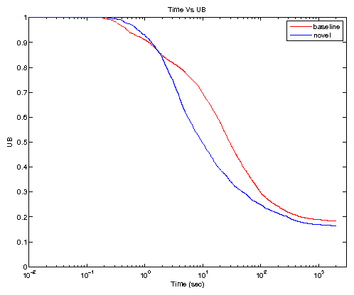
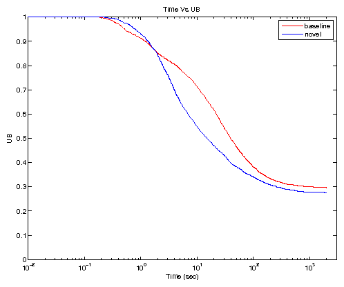
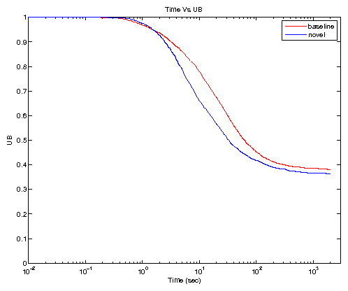
Hence we simply compare our two approaches and demonstrate that our algorithms are able to solve the problems in our data set. We demonstrate the convergence of the upper bound as a function of time in Fig 1. For each algorithm we produce as a function of time the proportion of the problems that algorithm has solved up to a satisfactory level. This level is computed as follows. We first compute the maximum lower bound between the two algorithms for a given problem which we denote as . We denote the least upper bound produced as a function of time as . We create a measure called the normalized gap which we define as . We show rapid convergence and that widest path computation helps improve performance.
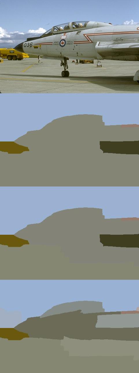
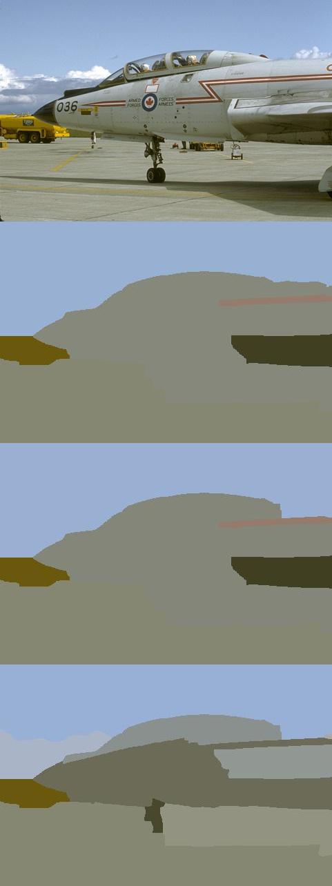
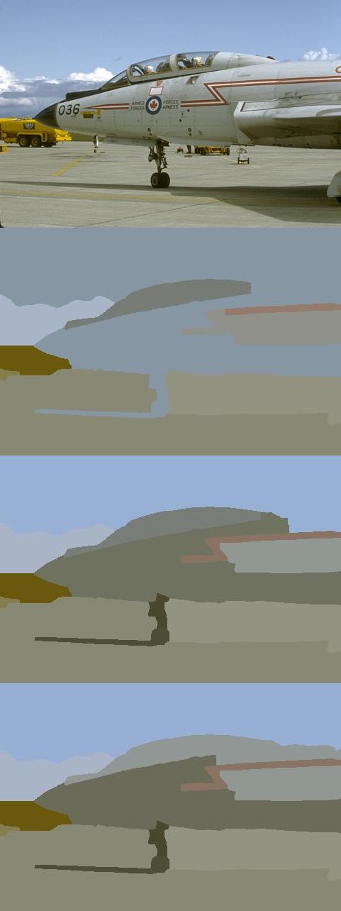
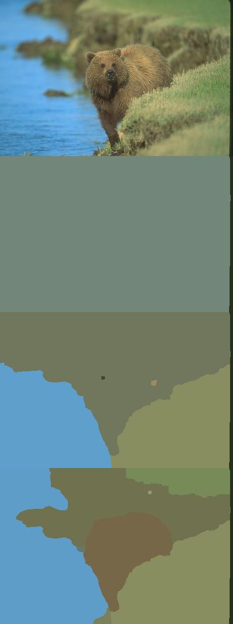
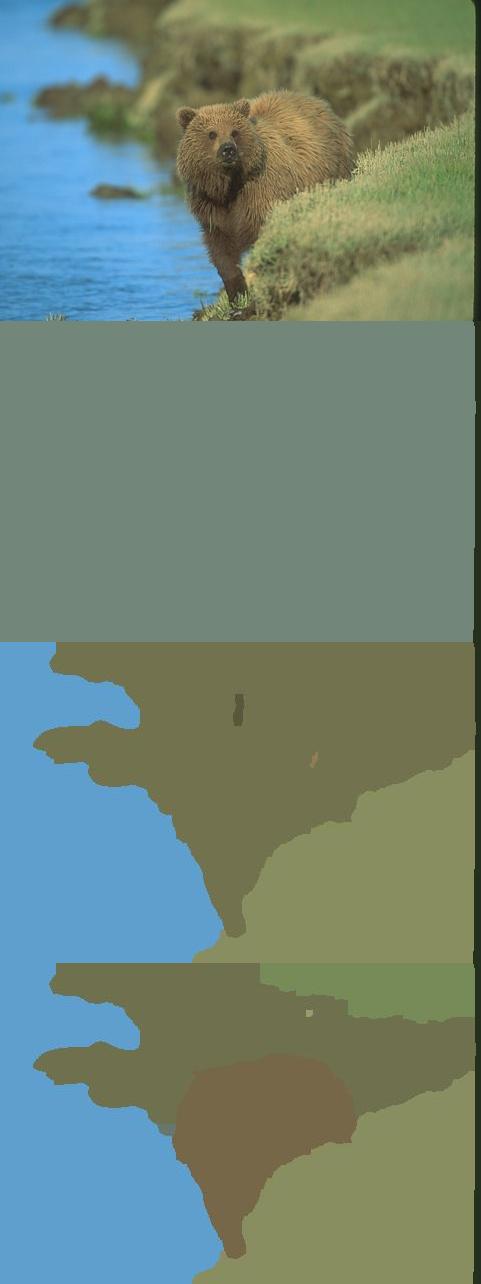
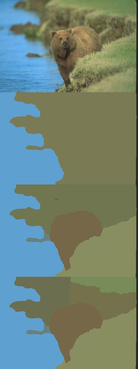
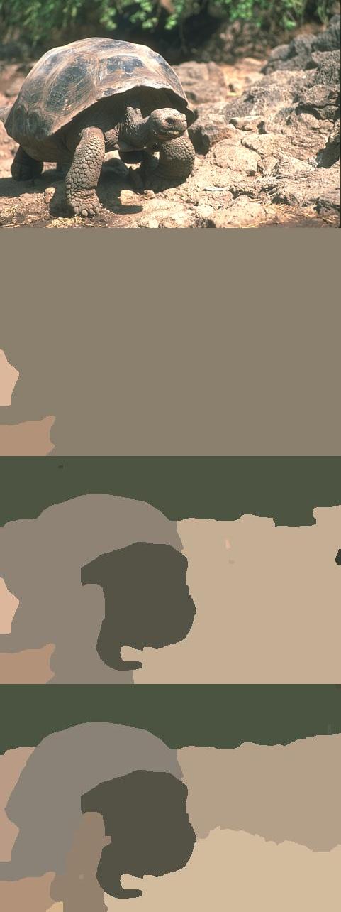
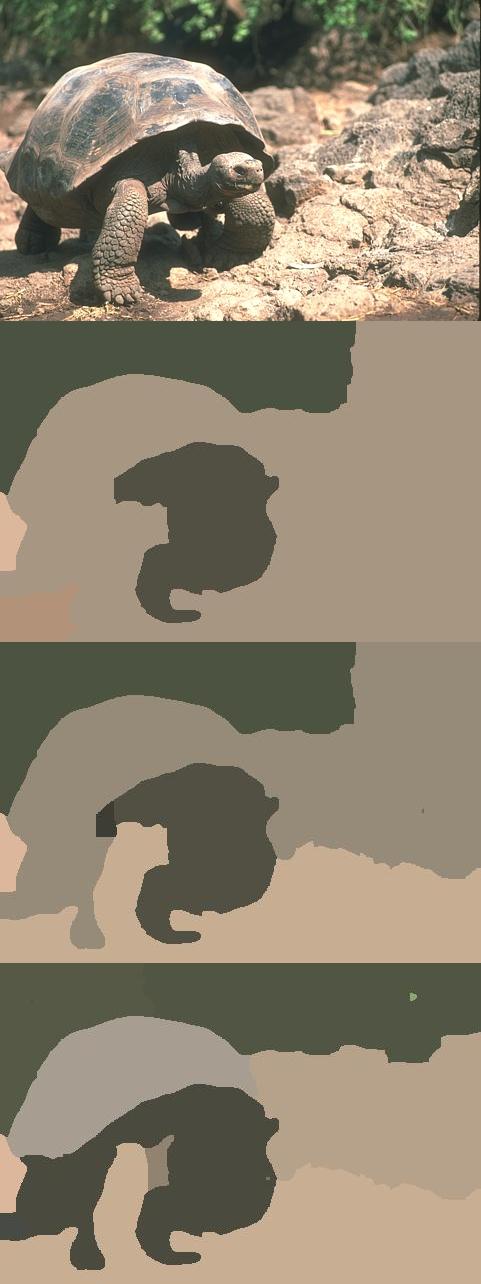
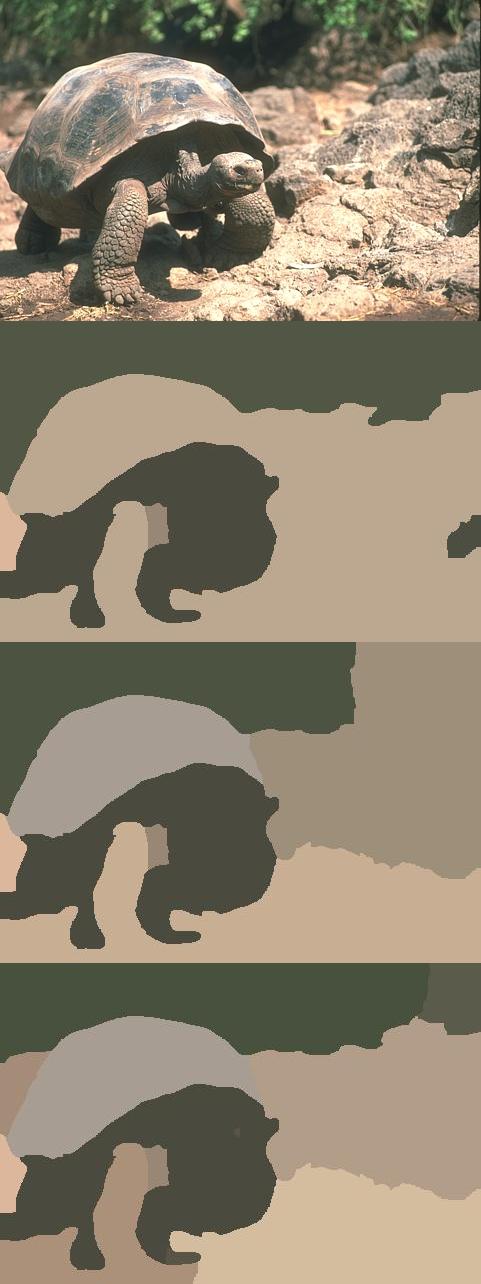
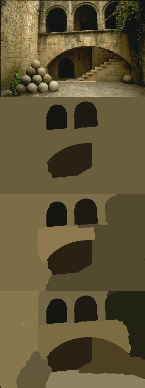
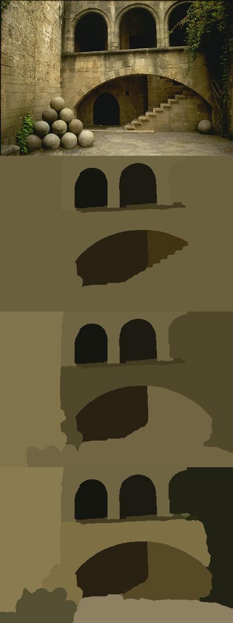
We now study some qualitative results from Alg 1 on various problems. For any given problem instance we produce the lowest cost multicut during optimization. Next for each component in the multicut we compute the mean color of the pixels in that component and color each pixel in the component with that color. Results are displayed in Fig 1. We observe large qualitative improvements in the results. However when smaller numbers of pairs are used we also often see tiny components created. However these often disappear and better boundaries emerge as more pairs are used.


References
- [1] B. Andres, J. H. Kappes, T. Beier, U. Kothe, and F. A. Hamprecht. Probabilistic image segmentation with closedness constraints. In Proceedings of the Fifth International Conference on Computer Vision (ICCV-11), pages 2611–2618, 2011.
- [2] B. Andres, T. Kroger, K. L. Briggman, W. Denk, N. Korogod, G. Knott, U. Kothe, and F. A. Hamprecht. Globally optimal closed-surface segmentation for connectomics. In Proceedings of the Twelveth International Conference on Computer Vision (ECCV-12), 2012.
- [3] B. Andres, J. Yarkony, B. S. Manjunath, S. Kirchhoff, E. Turetken, C. Fowlkes, and H. Pfister. Segmenting planar superpixel adjacency graphs w.r.t. non-planar superpixel affinity graphs. In Proceedings of the Ninth Conference on Energy Minimization in Computer Vision and Pattern Recognition (EMMCVPR-13), 2013.
- [4] Y. Bachrach, P. Kohli, V. Kolmogorov, and M. Zadimoghaddam. Optimal coalition structures in graph games. CoRR, abs/1108.5248, 2011.
- [5] S. Bagon and M. Galun. Large scale correlation clustering. In CoRR, abs/1112.2903, 2011.
- [6] F. Barahona. On the computational complexity of ising spin glass models. Journal of Physics A: Mathematical, Nuclear and General, 15(10):3241–3253, april 1982.
- [7] F. Barahona. On cuts and matchings in planar graphs. Mathematical Programming, 36(2):53–68, november 1991.
- [8] F. Barahona and A. Mahjoub. On the cut polytope. Mathematical Programming, 60(1-3):157–173, September 1986.
- [9] M. Deza and M. Laurent. Geometry of cuts and metrics, volume 15. Springer Science & Business Media, 1997.
- [10] M. E. Fisher. On the dimer solution of planar ising models. Journal of Mathematical Physics, 7(10):1776–1781, 1966.
- [11] S. Kim, S. Nowozin, P. Kohli, and C. D. Yoo. Higher-order correlation clustering for image segmentation. In Advances in Neural Information Processing Systems,25, pages 1530–1538, 2011.
- [12] D. Martin, C. Fowlkes, D. Tal, and J. Malik. A database of human segmented natural images and its application to evaluating segmentation algorithms and measuring ecological statistics. In Proceedings of the Eighth International Conference on Computer Vision (ICCV-01), pages 416–423, 2001.
- [13] X. Ren and J. Malik. Learning a classification model for segmentation. In Ninth IEEE International Conference on Computer Vision and Pattern Recognition (CVPR 2003), pages 10–17 vol.1, Oct 2003.
- [14] W.-K. Shih, S. Wu, and Y. Kuo. Unifying maximum cut and minimum cut of a planar graph. Computers, IEEE Transactions on, 39(5):694–697, May 1990.
- [15] D. Sontag, D. K. Choe, and Y. Li. Efficiently searching for frustrated cycles in MAP inference. In Proceedings of the Twenty-Eighth Conference on Uncertainty in Artificial Intelligence (UAI-12), pages 795–804, Corvallis, Oregon, 2012. AUAI Press.
- [16] D. Sontag, T. Meltzer, A. Globerson, T. Jaakkola, and Y. Weiss. Tightening lp relaxations for map using message passing. In Proceedings of the Twenty-Fourth Conference Annual Conference on Uncertainty in Artificial Intelligence (UAI-08), pages 503–510, july 2008.
- [17] J. Yarkony and C. Fowlkes. Planar ultrametrics for image segmentation. In Neural Information Processing Systems, 2015.
- [18] J. Yarkony, A. Ihler, and C. Fowlkes. Fast planar correlation clustering for image segmentation. In Proceedings of the 12th European Conference on Computer Vision(ECCV 2012), 2012.
Appendix A Computing Any Time Lower Bounds
In this section we construct a lower bound on the value of the optimal integer multicut that obeys all of the path inequalities. This lower bound is a function of and . Let denote the set of integer multicuts that obey all path inequalities. We use to denote a member of this set. We write formally below, along with the optimization over .
| (7) | |||
| (8) |
We now insert Lagrange multipliers corresponding to the constraints in the primal objective in Eq 5.
| (9) |
Observe that since must lie in KMCUT these multipliers have their global optimum at zero value. Let any particular setting of be chosen and denoted ,. Notice that this produces a lower bound on the true objective written below.
| (10) |
We now relax the constraint that the solution lie in to instead lie in the expanded space .
| (11) |
Solving for is exactly Planar Correlation Clustering which is known to be NP hard [4]. However [18] establishes that the times the value of the minimum 2-colorable multicut lower bounds the value of the optimal multicut. We use this fact to construct a lower bound on Eq 11 below.
| (12) |
Since computing the minimum 2-colorable multicut is solvable in we can produce a lower bound on the true objective given any setting of and which is written below.
| (13) |
Observe that at convergence of Alg 1,2 the value of and hence the value of the lower bound is exactly equal to that of the LP relaxation in Eq 5. During Alg1,2 we are able to produce a lower bound on our objective each time the dual LP solver produces a new setting of .
Appendix B Proof Cut
We now establish that at termination of Alg 1,2 lies in . First observe that given from Alg 1,2 we can greedily decrease values in until each and is a term in a tight constraint or is zero valued. This operation only effects terms associated with zero value in the primal objective.
We use these reduced and terms in the remainder of the proof. We call property that each and term is involved in a tight constraint or is zero valued .
To establish that we must establish the following for all cycles and edges in .
| (14) |
On any cycle inequality we refer to the edge on the right side of the inequality as the pivot edge. For short hand we use to refer to the set of all pairs of cycle and edge contained in the cycle. A member of is written as which denotes the cycle and pivot edge. We associate with non-overlapping subsets and whose union is . An element of denoted is in if and only if .
We now establish that all cycle inequalities are obeyed by first considering an cycle inequalities in and then in .
B.1 For
To establish that the cycle inequality associated with every pair we use proof by contradiction. Consider a violated cycle inequality over pair . We write this below.
| (15) |
Since then . Therefore we write Eq 15 without .
| (16) |
Recall that [17] establishes that for all thus the following is true.
| (17) |
Since is non-negative then the following is true which establishes a contradiction with Eq 16.
| (18) |
Therefor the cycle inequalities over members of are satisfied.
B.2 For
To establish that the cycle inequality associated with every pair is satisfied we use proof by contradiction. Consider a violated cycle inequality over pair . We write this below.
| (19) |
Observe that otherwise would cause a violation of . We now alter Eq 19 based on the observation that .
| (20) |
Clearly there must be a path inequality including edge that is tight otherwise is violated. Denote this path as and let it connect pair . We now write the expression for that path inequality and alter it.
| (21) | |||
| (22) |
| (23) |
Observe that the union of and is itself a path between a pair though one which may include edges multiple times. We denote this path as . Now observe the following.
| (24) | |||
However since path connects a pair then the sum of the edges on the path must be greater than or equal to one. Thus we have established a contradiction and therefore the pair is not associated with a violated cycle inequality.
B.3 Conclusion
Since every pair the associated cycle inequality is satisfied then all cycle inequalities are satisfied and thus .