Distributed User Association in Energy Harvesting Small Cell Networks: A Competitive Market Model with Uncertainty

Abstract

We consider a distributed user association problem in the downlink of a small cell network, where small cells obtain the required energy for providing wireless services to users through ambient energy harvesting. Since energy harvesting is opportunistic in nature, the amount of harvested energy is a random variable, without a priori known characteristics. We model the network as a competitive market with uncertainty, where self-interested small cells, modeled as consumers, are willing to maximize their utility scores by selecting users, represented by commodities. The utility scores of small cells depend on the amount of harvested energy, formulated as natures’ state. Under this model, the problem is to assign users to small cells, so that the aggregate network utility is maximized. The solution is the general equilibrium under uncertainty, also called Arrow-Debreu equilibrium. We show that in our setting, such equilibrium not only exists, but also is unique and is Pareto optimal in the sense of expected aggregate network utility. We use the Walras’ tatonnement process with some modifications in order to implement the equilibrium efficiently.

I Introduction

Due to the ever-increasing need for mobile services, we expect a massive growth in demand for wireless data delivery in the years to come. Facing an influx in data traffic, 5G networks are foreseen to alleviate this problem by deploying dense small cells to underlay the legacy macro cellular networks. This takes advantage from low-power and short-range base stations that operate (preferably) using the same radio spectrum as the macro base stations (MBSs) and offload macro cell traffic [1], [2]. However, deployment of small cell networks poses a variety of new challenges to system designers. Examples include synchronization [3], resource allocation [4], interference mitigation [5], handover management [6], and user association.

In this paper we address the problem of user association in a small cell network where the small cells are powered by the energy harvested from the ambient environment. The association to the MBS is not considered here. The motivations for the users to associate to the small cell base stations (SBSs) include smaller transmission power and the potential of better link quality and hence better coverage and capacity. Obviously, the users which are unable to associate to any of the SBSs, may associate with the MBS. As user association to the base stations is the focus of this paper, in the following we discuss some important related research works in more detail.

In [7], the authors propose a context-aware user-cell association approach for small cell networks that exploits the information about the velocity and trajectory of users. While taking the quality of service (QoS) requirements into account, matching theory is used to design a novel algorithm to solve the user association problem. Similarly, in [8], matching theory is applied to solve the user association problem in dense small cell networks. Reference [9] formulates the uplink user association as a college admission game and proposes an algorithm based on coalitional games to solve the problem. Joint user association and resource allocation is investigated in [10], where a belief propagation algorithm is proposed for joint user association, sub-channel allocation, and power control. Energy-efficient and traffic-aware user association are studied in [11] and [12], correspondingly. Both studies show the potential of exploiting the available context-aware information, for example, users’ measurements and requirements, as well as knowledge of the network, to associate the users in an energy- and spectrum-efficient way. A cross-layer framework for user association control in wireless networks is investigated in [13]. Reference [14] considers the problem of user association for load balancing. User association in conjunction with energy harvesting in small cell network is considered in [15]. Therein, stochastic geometry is used to develop a modeling framework for $K$-tier uplink cellular networks with RF energy harvesting from the concurrent cellular transmissions.

I-A Motivation and Contribution

In a vast majority of previous research works, the proposed user association scheme is centralized or only partially distributed, which necessitates the availability of global channel state information (CSI) at a central node, resulting in high computational cost and/or overhead. Therefore, it becomes imperative to develop distributed user association schemes that are able to cope with information shortage. Furthermore, in order to maintain low cost, small cells need to be self-organizing and self-healing. Specifically, the required energy of small cells is desired to be harvested locally from the ambient environment [16], rather than being provided by using a fixed power supply (which might require frequent recharging), or through energy transfer from a power beacon (which might result in transfer costs and energy wastes). This sort of energy-independency is in particular feasible in small cell network, since small cells normally provide limited services to a small number of users; that is, the energy obtained through energy harvesting might suffice to satisfy users’ requirements. However, since energy harvesting is opportunistic in general, uncertainty is a natural attribute of the amount of residual energy in small cells. In the presence of uncertainty, distributed user association becomes even more challenging, since assignment is performed before any information regarding the amount of energy in each small cell is disclosed. Moreover, it should be mentioned that, in a large body of previous literature, the proposed user association method is designated for a specific energy harvesting model, for example, random Poisson process [17] or Bernoulli energy arrival [18]. Furthermore, the proposed approach depends highly on a specific performance metric, so that by a small change in the utility function, the approach is not applicable anymore.

In the above context, we develop a new theoretical framework to analyze the user assignment problem in small cell networks, while taking the aforementioned issues into account. We assume that each SBS has the statistical CSI of all users with respect to itself, i.e., the local CSI; nevertheless, in contrast to centralized approaches, no central controller is in possession of global CSI. Moreover, the energy of each small cell is harvested on-site through its own energy harvesting units. In order to cope with the hidden uncertainty raised by allowing opportunistic energy harvesting, we model the network as a competitive market with uncertainty. More precisely, small cells are represented by consumers, which selfishly aim at maximizing their utility scores by selecting users, despite being uncertain about the amount of harvested energy. Under this model, we show the existence of equilibrium and describe its characteristics, including optimality and uniqueness. Moreover, based on the well-known Walras’ tatonnement process, we develop an approach to implement equilibrium efficiently. In sharp contrast to previous works, our solution is generic in the sense that it does not rely on a specific energy harvesting model, and can be used in conjunction with a variety of performance metrics. Moreover, apart from user association, our proposed model is applicable to a variety of resource allocation problems under uncertainty. An instance is the channel selection problem in cognitive radio networks for secondary users, where the statistics of channel availability is unknown a priori. In Table I, we compare some user association methods in heterogeneous networks in conjunction with energy harvesting.

TABLE I: User Association in Conjunction with Energy Harvesting in Heterogeneous Networks

	Approach	Metric	Uncertainty	Information	Concentration	Specific Energy Model
[19]	Gradient Descent	User-Acceptance Rate	No	Global CSI	Centralized	No
[18]	Stochastic Geometry	Traffic Offloading	No	Global CSI	Centralized	Yes
[17]	Stochastic Geometry	Aggregate Throughput	No	Global CSI	Centralized	Yes
[20]	Convex Optimization	Delay-Load Trade-off	No	Local CSI	Distributed	Yes
[21]	Convex Optimization	Delay-Energy Balance	No	Global CSI	Centralized	Yes
[22]	Convex Optimization	Energy Efficiency	No	Global CSI	Centralized	Yes
Our Work	Exchange Economy	Aggregate Throughput	Yes	Local CSI	Distributed	No

I-B Paper Organization

The rest of the paper is organized as follows. In Section II, we describe the system model and formulate the user association problem. In Section III, we briefly introduce competitive market model and exchange economy under uncertainty, by providing some basic definitions and results. We also describe the Walras’ tatonnement procedure. In Section IV, we model the user association problem as an exchange economy under uncertainty, and we characterize the equilibrium. We also show that in an exchange economy with indivisible goods, the demand calculation can be formulated and solved as a static knapsack problem. Section V includes numerical results. Section VI summarizes the paper and adds some concluding remarks.

I-C Notation

Throughout the paper we denote a set and its cardinality by a unique letter, and distinguish them by using calligraphic and italic fonts, such as $\mathcal{A}$ and $A$, respectively. Matrices are shown by bold upper case letters, for instance $\mathbf{A}$. Moreover, $\mathbf{A}_{l}$ denotes the $l$-th row of matrix $\mathbf{A}$. $[\mathbf{A}]_{l,m}$ stands for the element of matrix $\mathbf{A}$ located at $l$-th row and $m$-th column. Unit vectors are shown by bold lower case letters, for example, a. The Hadamard (element-wise) product of two matrices $\mathbf{A}$ and $\mathbf{B}$ is shown as $\mathbf{A}{\circ}\mathbf{B}$. Furthermore, by $\mathbf{A}=\mathbf{B^{{}^{\circ\frac{1}{2}}}}$ we mean that matrix $\mathbf{B}$ is the element-wise square of matrix $\mathbf{A}$.

II System Model and Problem Formulation

We consider a small cell network consisting of an MBS, a set $\mathcal{M}=\{1,...,M\}$ of users and a set $\mathcal{N}=\{1,...,N\}$ of small cells. Every small cell $n\in\mathcal{N}$ provides wireless services to a set of users, $\mathcal{M}_{n}\subseteq\mathcal{M}$. Define the assignment matrix $\mathbf{X}=\left[x_{nm}\right]_{N\times M}$. Traditionally, each user can associate to a single SBS; that is,

$$\begin{matrix}x_{nm}\in\left\{0,1\right\},&\forall~{}m\in\mathcal{M},n\in\mathcal{N}\end{matrix},$$ (1)

and,

$$\begin{matrix}\sum_{n\in\mathcal{N}}x_{nm}=1,&\forall~{}m\in\mathcal{M}\end{matrix}.$$ (2)

Multiple simultaneous associations, however, would enhance the system throughput and reduce the outage ratio, particularly for cell edge users [1]. Therefore, in this paper, we develop a framework that can also be applied to the continuous case, where, from every user $m\in\mathcal{M}$, a fraction $x_{nm}\in\left[0,1\right]$ is assigned to small cell $n\in\mathcal{N}$; that is,

$$\begin{matrix}x_{nm}\in\left[0,1\right],&\forall~{}m\in\mathcal{M},n\in\mathcal{N}\end{matrix},$$ (3)

where also (2) holds. The fraction $x_{nm}$ can be interpreted as some sort of handover: Small cell $n$ provides $x_{nm}$ fraction of the required spectrum resources for user $m$, or supports it for $x_{nm}$ fraction of the transmission time. As mentioned before, by $\mathbf{X}_{n}$, we denote the $n$-th row of matrix $\mathbf{X}$, which provides information about the users assigned to small cell $n\in\mathcal{N}$. Clearly, for the discrete and continuous cases, we have $\mathbf{X}_{n}\subset\{0,1\}^{M}$ and $\mathbf{X}_{n}\subset\left[0,1\right]^{M}$, respectively. In our work, we distinguish those results and algorithms that cannot be directly applied to the continuous model, and provide substitute solutions.

We assume that energy harvesting is independent across small cells. In other words, each small cell $n\in\mathcal{N}$ has its own energy harvesting units, so that by utilizing these units, its required energy is locally obtained from the ambient environment. The energy is then spent by the small cell to serve its assigned users. We assume that the network operates in two consecutive time intervals. In the first interval, user association and scheduling decisions are made; that is done while SBSs are harvesting the energy, but before any information about the amount of harvested energy is disclosed. Transmissions are performed in the second interval, after each SBS knows the exact amount of harvested energy. In general and regardless of the specific method, energy harvesting is opportunistic; hence, for every small cell, the amount of harvested (or residual) energy is random in nature. Therefore, we model the residual energy as a random variable. We do not make any assumption on the probability density function of this random variable. For each small cell $n\in\mathcal{N}$, we refer to every possible level of residual energy as one state, which belongs to a finite set of integer values $\mathcal{S}_{n}$. The state space of the environment can be then written as

$$\mathcal{S}=\bigotimes_{n=1}^{N}\mathcal{S}_{n},$$ (4)

where $\bigotimes$ is the Cartesian product. From (4), at each time, the nature’s state is defined as the collection of residual energy levels of all small cells.

We assume that each small cell is provided with sufficient spectrum resources to guarantee orthogonal transmission to its assigned users; that is, inside every small cell, transmissions are corrupted only by zero-mean additive white Gaussian noise (AWGN) with variance $N_{0}$. For each small cell $n\in\mathcal{N}$, the intercell interference experienced by every user $m\in\mathcal{M}_{n}$, denoted by $I_{nm}\geq 0$, is regarded as noise and is assumed to be fixed and known. The average channel gain between user $m\in\mathcal{M}$ and small cell $n\in\mathcal{N}$ (including Rayleigh fading and path loss) is denoted by $h_{nm}$. We assume that each SBS $n\in\mathcal{N}$ is provided with statistical CSI of every link $n\to m$ for all $m\in\mathcal{M}$. We focus on downlink transmission. The model can be used in combination with various power allocation and/or transmission scenarios in each cell. As few examples, we consider the following transmission scenarios.

• Fixed-power transmission: Every SBS transmits to each of its assigned users with some fixed power $P_{n}$. Since the total available transmission power is a monotone increasing function of the bounded harvested energy, every SBS is able to serve only a limited number of users. Let $P^{(s)}_{n}\in\mathcal{R}_{+}-\left\{\infty\right\}$ be the total available power at small cell $n\in\mathcal{N}$. Thus, at most $\alpha^{(s)}_{n}=\left\lfloor\frac{P^{(s)}_{n}}{P_{n}}\right\rfloor$ users can be served. If $\alpha^{(s)}_{n}<M_{n}$, then a subset of users, say $\mathcal{M}^{\prime}_{n}\subset\mathcal{M}_{n}$ has to be selected to be served, where $M^{\prime}_{n}\leq\alpha^{(s)}_{n}$. For each $m\in\mathcal{M}_{n}$, the achievable transmission rate is given by

  $$r_{nm}(h_{nm})=\log\left(1+\frac{P_{n}h_{nm}}{N_{0}+I_{nm}}\right).$$ (5)

  To define $\mathcal{M}^{\prime}_{n}$, each small cell orders the assigned users based on achievable transmission rate. Let $\mathcal{M}_{n,\max}^{(s)}\subseteq\mathcal{M}_{n}$ denote the set of $\alpha^{(s)}_{n}$ users that yield the largest transmission rates; that is, the first $\alpha^{(s)}_{n}$ users in the descending ordering of achievable transmission rates are collected in the set $\mathcal{M}_{n,\max}^{(s)}$. The utility of small cell $n$ from user $m$ is then defined as

  $$u_{nm}^{(s)}=\begin{cases}r_{nm}&m\in\mathcal{M}_{n,\max}^{(s)}\\ 0&\text{o.w.}\end{cases}.$$ (6)

  That is, only the best $\alpha^{(s)}_{n}$ users are served, which thus yields benefit.

• Full-power transmission: Each SBS can broadcast the data with the entire available power to all its assigned users, in case every user in a small cell is interested in receiving all information. Such scenario arises often in multimedia transmission, online gaming, and file downloading. In this case, at every state $s$, the utility of SBS $n$ from every user $m\in\mathcal{M}_{n}$ is given by (5) after replacing $P_{n}$ with $P^{(s)}_{n}$.

• Equal-power transmission: Every SBS transmits to its entire assigned users with equal power; that is, the available power is shared by all users equally. Then, at each state $s$, the utility is given by (5) with $P_{n}=P^{(s)}_{n}/M_{n}$.

Regardless of the transmission model, for every small cell $n\in\mathcal{N}$, we define the utility function $u_{n}:\{0,1\}^{M}\to\mathcal{R}_{+}-\left\{\infty\right\}$ (or $\left[0,1\right]^{M}\to\mathcal{R}_{+}-\left\{\infty\right\}$, for the continuous case) as the aggregate data rate experienced by the users assigned to that specific small cell. Formally,

$$u_{n}^{(s)}(\mathbf{X}_{n})=\sum_{m\in\mathcal{M}}u_{nm}^{(s)}[\mathbf{X}]_{n,m},$$ (7)

where $[\mathbf{X}]_{n,m}$ stands for the element of matrix $\mathbf{X}$ located at $n$-th row and $m$-th column.

As described before, user association is performed before energy harvesting; that is, at the time of user association, the amount of energy in each small cell, or, in other words, the nature’s state, is unknown. Under this uncertainty, the problem is to assign users to small cells in a distributed manner. By (7), for every small cell, the utility is state-dependent. Thus, the assignment matrix might be state-dependent as well. For any state $s\in\mathcal{S}$, we define the assignment matrix as $\mathbf{X}^{(s)}=\left[x_{nm}^{(s)}\right]_{N\times M}$. Let $\mathcal{X}$ be the set of all possible assignment matrices. Ideally, desired is to find $x_{nm}^{(s)}$ for all $m\in\mathcal{M}$ and $n\in\mathcal{N}$, so that at every state $s\in\mathcal{S}$, $\mathbf{X}^{(s)}$ is a solution of the following optimization problem:

$$\underset{\mathbf{X}^{(s)}\in\mathcal{X}}{\textup{maximize}}~{}\sum_{n\in\mathcal{N}}u_{n}^{(s)}\left(\mathbf{X}_{n}^{(s)}\right),$$ (8)

where for the discrete problem formulation, the problem is subject to (1) and (2), while (3) and (2) are the constraints for the continuous case.

However, since the nature’s state is unknown a priori, (8) is infeasible. Therefore, we opt for a less ambitious goal, described in the following. Assume that each small cell $n\in\mathcal{N}$ assigns probability vector $\mathbf{a}_{n}=\left(a_{n}^{(1)},...,a_{n}^{(S)}\right)$ to the set of states, $\mathcal{S}$. Then the expected utility yields

$$\bar{u}_{n}=\sum_{s=1}^{S}a_{n}^{(s)}u_{n}^{(s)}\left(\mathbf{X}_{n}^{(s)}\right).$$ (9)

We define the goal of user association as follows: For every state $s$, find an assignment matrix $\mathbf{X}$ that is a solution of the following optimization problem:

$$\underset{\mathbf{X}^{(s)}\in\mathcal{X}}{\textup{maximize}}~{}\sum_{n\in\mathcal{N}}\bar{u}_{n}\left(\mathbf{X}_{n}^{(s)}\right),$$ (10)

subject to (1), (2) for the discrete problem and (3), (2) for the continuous case. That is, the goal is defined as to maximize the aggregate expected utility of all SBSs.

III Exchange Economy with Uncertainty

According to the system model described in Section II, the problem is to assign users to small cells, before any information about energy harvesting is disclosed, in a way that the expected aggregate network utility is maximized. We aim at solving the problem in a distributed manner, by allowing every small cell to select users on its own. In doing so, the selfishness of small cells should be taken into account: Naturally, every small cell would like to select as many users as possible so as to maximize its own reward given by (7); nonetheless, the utility that can be achieved by each small cell, or, in other words, the contribution of each small cell to the network aggregate utility, is dictated by the amount of harvested energy in that small cell. The energy, however, is obtained through energy harvesting rather than a fixed power supply, and therefore can be regarded as a random variable whose realization is unknown a priori. Therefore, a mechanism is required to prevent SBSs from overestimating their energy resources while selecting users.

In this paper, we model the small cell network as a competitive market, accommodating an exchange economy with uncertainty. In this model, there is no producer. Consumers, each provided with an initial endowment, trade the available commodities while being ambitious to maximize their own utilities, and uncertain about the nature’s state. Under this model, the solution of problem (8) is the general equilibrium under uncertainty, also called Arrow-Debreu equilibrium.

In this section, we describe some basic notions of exchange economy and equilibrium under uncertainty. In Section IV, we describe our proposed model and analyze the formulated user association problem based on exchange economy.

III-A Exchange Economy

An exchange economy $\Omega$ consists of a set of consumers, $n\in\mathcal{N}$, and a set of commodities (goods), $m\in\mathcal{M}$. Let $\mathbf{I}=\left(i_{1},...,i_{M}\right)$ stand for the endowment of goods, with $i_{m}\in\mathcal{Z}$, $m\in\mathcal{M}$. For each consumer $n\in\mathcal{N}$, a bundle of commodities is a row matrix $\mathbf{X}_{n}\in\mathcal{Z}^{M}$ for indivisible goods and $\mathbf{X}_{n}\in\mathcal{R}_{+}^{M}$ for divisible goods. Each consumer is supplied with an initial endowment of commodities gathered in a row matrix $\mathbf{Q}_{n}\in\mathcal{Z}^{M}$ or $\textbf{Q}_{n}\in\mathcal{R}_{+}^{M}$ for indivisible and divisible goods, respectively, so that $\sum_{n\in\mathcal{N}}\mathbf{Q}_{n}=\mathbf{I}$. The model captures the idea of exchanging goods, without production, where the allocation of a given amount of each commodity implies its final consumption, associated with some utility score. A map $u_{n}:\mathcal{Z}^{M}\to\mathcal{R}$ (or $u_{n}:\mathcal{R}_{+}^{M}\to\mathcal{R}$, for divisible goods) is called a utility function on the commodity set $\mathcal{M}$ for every consumer $n\in\mathcal{N}$. Since utilities and initial endowments are the main blocks of exchange economy, we define any exchange economy $\Omega$ as $\Omega:\left\{u_{n},\mathbf{Q}_{n}\right\}_{n\in\mathcal{N}}$. In the following we define the monotonicity of utility functions.

Definition 1 (Monotonicity).

A utility function $u_{n}:\mathcal{Z}^{M}\to\mathcal{R}$ is monotone if for all $\mathbf{X}^{{}^{\prime}}_{n}\leq\mathbf{X}_{n},u_{n}(\mathbf{X}^{{}^{\prime}}_{n})\leq u_{n}\left(\mathbf{X}_{n}\right)$.

In a deterministic model of exchange economy, all information are provided to all individuals a priori, whereas under uncertainty, the nature can have different states, modeled as the outcomes of some random variable, unknown a priori. Let $\mathcal{S}$ denote the set of all possible states of the nature. We make the following assumption.

Assumption A1.

We assume the following on the set of space’s states, $\mathcal{S}$.

1. $\mathcal{S}$ is a finite set.

2. All elements in $\mathcal{S}$ are mutually exclusive.

3. $\mathcal{S}$ is exhaustive.

4. $\mathcal{S}$ is known to all individuals.

For $S$ states of nature and $M$ commodities, there exist $MS$ state contingent commodities. In simple words, state contingency means that a commodity $m$ in state $s$ is regarded as another commodity, say $m^{\prime}$, when the state changes to $s^{\prime}$. Arrow and Debreu show that the basic notions and theorems for a deterministic exchange economy with $M$ goods, for instance the two Welfare theorems [23], hold also for an exchange economy under uncertainty with $S$ possible space states and $M$ goods, simply by building a new exchange economy with $MS$ goods, i.e., state contingent commodities [24]. In such an economy, we define the allocation of a state contingent commodity as follows.

Definition 2 (Allocation).

An allocation of state contingent commodity $ms$, denoted by $x_{nm}^{(s)}\in\mathcal{Z}$ (or $x_{nm}^{(s)}\in\mathcal{R}_{+}$, for divisible goods), describes the number of units (or the amount) of commodity $m\in\mathcal{M}$ that can be consumed by individual $n\in\mathcal{N}$, if and only if state $s\in\mathcal{S}$ occurs.

Therefore, a state contingent allocation vector can be written as $\mathbf{X}_{n}=\left(x_{n1}^{(1)},...,x_{nM}^{(1)},...,x_{n1}^{(S)},...,x_{nM}^{(S)}\right)$. Throughout the paper, at each state $s\in\mathcal{S}$, we denote the vector of commodities allocated to consumer $n\in\mathcal{N}$ as $\mathbf{X}_{n}^{(s)}$. In a competitive market with uncertainty, the initial endowment of each consumer is in general random and state-dependent. Formally, initial endowments yields $\mathbf{Q}_{n}=\left(q_{n1}^{(1)},...,q_{nM}^{(1)},...,q_{n1}^{(S)},...,q_{nM}^{(S)}\right)$. Moreover, $\mathbf{Q}_{n}^{(s)}$ is the vector of initial endowments of consumer $n\in\mathcal{N}$ at state $s\in\mathcal{S}$. Every individual has to pay a price for every unit of each commodity under each state. That is, a price $p_{m}^{(s)}$ has to be paid for every unit of a state contingent commodity $ms$, $m\in\mathcal{M}$ and $s\in\mathcal{S}$. Hence we denote the price vector by $\mathbf{P}=\left(p_{1}^{(1)},...,p_{M}^{(1)},...,p_{1}^{(S)},...,p_{M}^{(S)}\right)\in\mathcal{R}_{+}^{MS}$. Also, at each state $s$, the price vector is denoted by $\mathbf{P}^{(s)}\in\mathcal{R}_{+}^{M}$.

Now assume that consumer $n\in\mathcal{N}$ assigns probability vector $\mathbf{a}_{n}=\left(a_{n}^{(1)},...,a_{n}^{(S)}\right)$ to the set of states, $\mathcal{S}$. Consumers do not have to agree on a specific probability distribution. So, the expected utility is given by (9). Then, consumers’ preferences, denoted by $\succeq_{n}$ on $\mathcal{R}_{+}^{MS}$, $n\in\mathcal{N}$, are state-dependent and can be represented as

$$\mathbf{X^{\prime}}_{n}^{(s)}\succeq_{n}\mathbf{X}_{n}^{(s)}\Leftrightarrow\bar{u}_{n}^{(s)}\left(\mathbf{X^{\prime}}_{n}^{(s)}\right)\geq\bar{u}_{n}^{(s)}\left(\mathbf{X}_{n}^{(s)}\right).$$ (11)

Let the utility of each consumer $n\in\mathcal{N}$ from commodity $m\in\mathcal{M}$ be denoted by $u_{nm}$. Then, at state $s$, its net benefit yields

$$v_{n}^{(s)}\left(\mathbf{X}_{n}^{(s)},\mathbf{P}^{(s)}\right)=\sum_{m\in\mathcal{M}}u_{nm}\left[\mathbf{X}_{n}^{(s)}\right]_{1,m}-\sum_{m\in\mathcal{M}}\left[\mathbf{P}^{(s)}\right]_{1,m}.$$ (12)

At each state $s\in\mathcal{S}$, given the prices of commodities, the demand correspondence of a consumer $n\in\mathcal{N}$ is defined as

$$\mathcal{D}_{n}^{(s)}\left(\mathbf{P}^{(s)}\right):=\left\{\mathbf{X}_{n}^{(s)}|v_{n}^{(s)}\left(\mathbf{X}_{n}^{(s)},\mathbf{P}^{(s)}\right)\geq v_{n}^{(s)}\left(\mathbf{X^{\prime}}_{n}^{(s)},\mathbf{P}^{(s)}\right)\right\},$$ (13)

where $\mathbf{X}_{n}^{(s)}\in\mathcal{Z}^{M}$ and $\mathbf{X}_{n}^{(s)}\in\mathcal{R}_{+}^{M}$ for indivisible and divisible commodities, respectively. Thus the final consumption depends on the state of nature; this means that same quantities of a given commodity might result in different utility scores in different states. We now define gross substitutes, which is an important concept in exchange economy.

Definition 3 (Gross Substitutes).

Let $\mathcal{D}_{n}\left(\mathbf{P}\right)$ be the demand correspondence for consumer $n$, given price vector $\mathbf{P}$, defined by (13). A utility function $u_{n}:\mathcal{Z}^{M}\to\mathcal{R}$ (or $u_{n}:\mathcal{R}^{M}_{+}\to\mathcal{R}_{+}$) satisfies the gross substitutes condition if for any two price vectors $\mathbf{P}$ and $\mathbf{P}^{\prime}$ where $\mathbf{P}^{\prime}\geq\mathbf{P}$, and for any $\mathbf{X}_{n}\subset\mathcal{D}_{n}\left(\mathbf{P}\right)$, there exists $\mathbf{X}^{\prime}_{n}\subset\mathcal{D}_{n}\left(\mathbf{P}^{\prime}\right)$ such that for all $m\in\mathcal{M}$, $x_{nm}=x^{\prime}_{nm}$ if $p_{m}=p^{\prime}_{m}$.

In words, gross substitutes means that if a consumer demands a bundle of commodities and the prices of some good increase, it would still demand the goods in that bundle whose prices did not change.

Next we state some conventional assumptions on the utility function.

Assumption A2.

For all $n\in\mathcal{N}$ and $u_{n}:\mathcal{R}_{+}^{M}\to\mathcal{R}$,

1. $u_{n}$ is continuous,

2. $u_{n}$ is increasing,

3. $u_{n}$ is concave, and

4. $\mathbf{Q}_{n}>0$.

Assumption A3.

For all $n\in\mathcal{N}$ and $u_{n}:\mathcal{Z}^{M}\to\mathcal{R}$,

1. $u_{n}$ is monotone, and

2. it satisfies the gross substitutes condition.

We gather all individual demands $\left[\mathbf{X}_{n}\right]_{1\times M}$, $n\in\mathcal{N}$, in a matrix $\left[\mathbf{X}\right]_{N\times M}$. Each consumer selects its consumption so as to maximize its expected utility; that is, consumer $n\in\mathcal{N}$ solves for

$$\begin{aligned} \underset{\mathbf{X}_{n}}{\textup{maximize}}&~{}~{}\bar{u}_{n}(\mathbf{X}_{n})\\ \textup{s.t.}~{}~{}~{}~{}&\mathbf{P}\cdot\mathbf{X}_{n}\leq\mathbf{P}\cdot\mathbf{Q}_{n}\end{aligned},$$ (14)

where $\mathbf{P}.\mathbf{X}_{n}\leq\mathbf{P}.\mathbf{Q}_{n}$ is the budget constraint. In general, the budget set writes

$$\mathcal{B}_{n}(\mathbf{P})=\left\{\mathbf{X}_{n}:\mathbf{P}\cdot\mathbf{X}_{n}\leq\mathbf{P}\cdot\mathbf{Q}_{n}\right\}.$$

At some price vector $\mathbf{P}$ and for a good $m\in\mathcal{M}$, the excess demand is defined as

$$z_{m}(\mathbf{P})=\sum_{n\in\mathcal{N}}d_{nm}(\mathbf{P},\mathbf{P}.\mathbf{Q}_{n})-\sum_{n\in\mathcal{N}}q_{nm},$$ (15)

where $d_{nm}(\cdot)$ is the demand of consumer $n\in\mathcal{N}$ for good $m\in\mathcal{M}$. Now we define Pareto optimal allocation.

Definition 4 (Feasible Allocation).

In an exchange economy $\Omega$, an allocation $\mathbf{X}$ is feasible if $\sum_{n\in\mathcal{N}}\mathbf{X}_{n}\leq\sum_{n\in\mathcal{N}}\mathbf{Q}_{n}$.

Definition 5 (Pareto Optimal Allocation).

A feasible allocation $\mathbf{X}$ is Pareto optimal if there is no other feasible allocation $\mathbf{X}^{\prime}$ such that $\bar{u}_{n}(\mathbf{X^{\prime}}_{n})\geq\bar{u}_{n}(\mathbf{X}_{n})$ for all $n\in\mathcal{N}$ with strict inequality for some $n\in\mathcal{N}$.

Before we proceed to the next section, we state two lemmas that we use later to prove some characteristics of our proposed solution.

Lemma 1 ([25]).

Additive concave and separable additive utility functions satisfy the gross substitutes property.

Lemma 2 ([26]).

If each individual has a utility function satisfying the gross substitutes condition, then both the individual and aggregate excess demand functions satisfy gross substitutes condition as well.

III-B Arrow-Debreu Equilibrium

The outcome of a deterministic competitive market (exchange economy) is the general equilibrium, also called Walrasian equilibrium. In an uncertain environment, however, deterministic equilibrium is insufficient, and extensions should be provided. One extension is the general equilibrium under uncertainty, also called Arrow-Debreu equilibrium. In this notion of equilibrium, prices are not state contingent, whereas allocations are. In other words, commitments are made before the state is known, at date 0, while allocations follow after revealing the state, at date 1. The sequence of events in an Arrow-Debreu model is described in Algorithm 1.

Algorithm 1 Arrow-Debreu Sequence of Events

1:  At $t=0$, nature’s state is unknown. Commitments are however made in this stage, i.e., under the uncertainty. This means that, at $t=0$, each agent $n\in\mathcal{N}$ determines its optimal demand and buys $x_{nm}^{(s)}$ units (amount) of each good $m\in\mathcal{M}$ if state $s\in\mathcal{S}$ occurs, and signs a contract in which it commits to pay the price.

2:  At $t=1$, the state $s$ is revealed. The contracts under state $s$ are executed, and all other contracts become void; that is, each individual receives the purchased goods under current state and pays the associated price.

For a competitive market, the Arrow-Debreu equilibrium is defined as follows [24].

Definition 6 (Arrow-Debreu Equilibrium).

An allocation matrix $\mathbf{X}$, together with a price vector $\mathbf{P}$ are an Arrow-Debreu equilibrium if

1. $\forall n\in\mathcal{N}$, $\mathbf{X}_{n}$ maximizes $\bar{u}_{n}$ on $\mathcal{B}_{n}$;

2. Market clears, that is, for all $m\in\mathcal{M}$

   $$\sum_{n\in\mathcal{N}}x_{nm}=\sum_{n\in\mathcal{N}}q_{nm}.$$ (16)

Now we are in a position to describe some results regarding the existence and optimality of Arrow-Debreu equilibrium. It should be mentioned that the following results are originally developed for the outcome of a deterministic competitive market model, i.e., Walrasian equilibrium [25]. Nonetheless, in [24], it is shown that these results hold also for competitive market with uncertainty, with its outcome being Arrow-Debreu equilibrium.

Theorem 1 (Existence of Arrow-Debreu Equilibrium).

Arrow-Debreu equilibrium $\left(\mathbf{X},\mathbf{P}\right)$ exists for

1. an economy with divisible goods that satisfies Assumption (A2) [23], and

2. an economy with indivisible goods that satisfies Assumption (A3) [25].

Theorem 2 (Optimality of Arrow-Debreu Equilibrium).

Let $\left(\mathbf{X},\mathbf{P}\right)$ be an Arrow-Debreu equilibrium. Then,

1. the allocation $\mathbf{X}$ is Pareto optimal for an economy $\Omega$ with divisible goods if Assumption A2-b holds [25].

2. the allocation $\mathbf{X}$ is Pareto optimal for an economy $\Omega$ with indivisible goods if Assumption A3-a holds [23];

Theorem 3 (Uniqueness of Arrow-Debreu Equilibrium [26]).

For an economy $\Omega$ with divisible goods, if the aggregate excess demand function $z(\cdot)$ satisfies the gross substitutes condition, then the economy has at most one Arrow-Debreu equilibrium, i.e., $z\left(\mathbf{P}\right)=0$ has at most one (normalized) solution.

In the next section we describe a method to achieve equilibrium in an exchange economy.

III-C Walras’ Tatonnement Process

In previous sections, we discussed an exchange economy under uncertainty, and described the notion of equilibrium in such setting. Still, it is important to describe how the equilibrium prices are reached, or, in other words, how equilibrium is implemented. To this end, Walras developed a price adjustment process, namely Walras’ tatonnement, known also as Walrasian auction. The process requires a coordinator, called Walrasian auctioneer, which, at each round, announces the prices, starting at some random initial point. Afterwards, consumers disclose their demands at those prices, so that the auctioneer can adjust prices to demands. The process continues until market clears; that is, when a set of prices yields a demand equal to supply. At this point, prices and demands are final, and the auction process terminates, i.e., trade occurs [27]. Let $z\left(\mathbf{P}\right)$ be the excess demand given price vector $\mathbf{P}$. For divisible goods, the price adjustment rule for the auctioneer is [26]

$$\mathbf{P}(t+1)=\mathbf{P}(t)+\alpha z\left(\mathbf{P}(t)\right),$$ (17)

for a sufficiently small $\alpha>0$. Clearly the only stationary points of this process are prices $\mathbf{P}$ at which $z(\mathbf{P})=0$, i.e., equilibrium prices [26]. For indivisible goods, the price adjustment rule yields [28]

$$\mathbf{P}(t+1)=\mathbf{P}(t)+\alpha\Delta\left(\mathbf{P}(t)\right),$$ (18)

where $\Delta=\left(\delta_{1},...,\delta_{M}\right)$, and $\delta_{m}=1$ if $m\in\mathcal{M}$ is in excess demand and zero otherwise. The procedure is summarized in Algorithm 2. Note that conventional auction methods such as VCG mechanism [29], although exhibiting nice properties such as incentive-compatibility, are not guaranteed to converge to an equilibrium in an exchange economy with uncertainty. Thus, we use the Walras’ tatonnement process and prove its convergence in our setting.

Algorithm 2 Walras’ Tatonnement Process

1:  Select the price adjustment factor $\alpha\to 0$.

2:  Initialize the price of each good, $p_{m}\to 0$, $m\in\mathcal{M}$.

3:  repeat

4:     

• Auctioneer announces the prices.

• Each consumer announces its demand.

• Auctioneer observes excess demands.

• Auctioneer adjusts the prices using (17) or (18).

5:  until Market clears.

The following theorem describes the convergence characteristics of Walras’ tatonnement process.

Theorem 4 (Convergence of Walras’ Tatonnement).

Consider an economy $\Omega$ and suppose that $\mathbf{P}$ is a Walrasian (or Arrow-Debreu) equilibrium price vector.

• Suppose that goods are divisible and the aggregate excess demand function $z(\cdot)$ satisfies the gross substitutes condition. Then the tatonnement process with price adjustment rule (17) converges to the relative prices of $\mathbf{P}$ as $t\to\infty$ for any initial condition $\mathbf{P}(0)$ [26].

• Suppose that goods are indivisible and users’ preferences satisfy the gross substitutes condition. Then the tatonnement process with price adjustment rule (18) converges to the relative prices of $\mathbf{P}$ in a finite number of steps for initial prices $\mathbf{P}(0)\to\mathbf{0}$ [25], [28].

IV Competitive Market Model of Small Cell Networks

As described shortly in Section III, in this paper, we model the small cell network by an exchange economy under uncertainty. The joint residual energy level of small cells corresponds to nature’s state, which varies randomly and is unknown a priori, hence counts as the source of uncertainty. Consumers and commodities, on the other hand, represent respectively small cells and users. This implies that in our market model only one unit of each commodity exists. As described in Section III-A, in an exchange economy, goods can be divisible or indivisible; this generality of our model allows us to associate every user to a single SBS, or let it be served by multiple SBSs. We assume that the initial user endowment of each small cell is determined by the MBS. For the continuous case, we assume that initially the MBS assigns to each SBS some positive fraction of each user. Although this can be done simply at random, a smarter choice is to allocate initial endowments based on the possible amount of harvested energy. The reason is as follows. According to the competitive market model described in Section III-A, each SBS has to pay a price for each user. Larger initial endowment thus might correspond to higher budget, thereby higher purchase ability; that is, it is reasonable to allocate larger endowments, thus larger budget, to those small cells that might harvest larger amount of energy and vice versa. In the case of ambient energy harvesting, this could be done, for instance, by using weather history and/or forecast.

At state $s$, the net utility of small cell $n\in\mathcal{N}$ yields:

$$v_{n}^{(s)}=\sum_{m\in\mathcal{M}}u_{nm}^{(s)}x_{nm}^{(s)}-\sum_{m\in\mathcal{M}}p_{m}^{(s)}x_{nm}^{(s)},$$ (19)

where $u_{nm}^{(s)}$ is defined based on the transmission model, as described previously in Section II. Moreover, $x_{nm}^{(s)}$ is the fraction of user $m$ associated to small cell $n$ if state $s$ occurs, where $x\in\{0,1\}$ and $x\in\left[0,1\right]$ for discrete and continuous cases, respectively. In cases of fixed-power and equal-power transmission models (see Section II), for every SBS $n$, the utility achieved by serving any user $m\in\mathcal{M}$ depends on the set of assigned user, $\mathcal{M}_{n}$, which is unknown when the optimization problem (14) is solved by the SBS. In order to solve this issue, we modify the defined utility functions, by assuming the following: 1) In fixed-power transmission, each SBS $n$ transmits to all (not only a subset of) its assigned users $m\in\mathcal{M}_{n}$ with fixed power $P_{n}$. By using this approximation, the optimization problem actually maximizes an upper-bound of the expected utility. 2) In equal-power transmission, each SBS $n$ transmits to all its assigned users with power $P_{n}^{(s)}=P^{(s)}_{n}/M$. By using this approximation, the optimization problem actually maximizes a lower-bound of the expected utility. In Section V-B and by means of numerical evaluations, we show that such approximations perform well. For the full-power transmission model no approximation is required.

Based on the model of exchange economy under uncertainty, users are assigned to small cells before the nature’s state is known, i.e., before the uncertainty is revealed. Thus, every small cell has to pay the price of each one of its selected users, regardless of being able to appropriately serve that user or not. In other words, even if low (or no) benefit can be made from some user at the occurred state (due to lack of energy), the price of that specific user has to be paid. By (19), in such cases, the net utility of a small cell can become even negative. This mechanism prevents the SBSs from overestimating their ability to harvest the energy, and guides the system towards optimality and truthfulness. Moreover, this implies that the utility score of each individual depends on the energy level, or in other words, the state of nature, which is a random variable (see Section II). In essence, the difference between conventional deterministic competitive market models (for an example in the context of channel assignment, see [28]) and that under uncertainty is as follows: In the latter, every small cell (consumer) pays a price for every user (unit of commodity) before it knows its actual energy level (state of the nature), whereas in the former, all information are given a priori, excluding all forms of uncertainty. The following theorem describes the equilibrium’s characteristics in our setting.

Theorem 5.

Arrow-Debreu equilibrium exists in our setting and is Pareto optimal. Moreover, it is unique for the case where a user can be assigned multiple SBSs.

Proof:

IV-1 Existence and Pareto optimality

1. Divisible goods: The utility function defined by (7) is the sum of continuous, increasing and concave functions. Therefore Assumption A2-a through A2-c holds. On the other hand, A2-d holds due to our system model described in Section IV. Hence, by Theorem 1-a, Arrow-Debreu equilibrium exists, which is also Pareto optimal due to Theorem 2-a.

2. Indivisible goods: The utility function defined by (7) is additive separable, since it is completely specified by the values it assigns to singletons. Then, by Lemma 1, it satisfies the gross substitutes condition. As it is also monotone, it satisfies the axioms of Assumption A3. Then, by Theorem 1-b, Arrow-Debreu equilibrium exists, which is also Pareto optimal due to Theorem 2-b.

IV-2 Uniqueness

Since the utility function given by (7) is additive separable, it satisfies the gross substitutes property by Lemma 1. Then, by Lemma 2, the excess demand function also satisfies the gross substitutes property. The result therefore follows by Theorem 3. ∎ The Walras’ tatonnement process described in Section III-C can be used to implement equilibrium. The entire user association procedure is summarized in Algorithm 3.

Algorithm 3 User Selection with Exchange Economy Model under Uncertainty

1:  At $t=0$, when the amount of harvested energy at each node is unknown:

• The MBS assigns each SBS an initial (probably state-dependent) endowment, either using available information or at random or simply equally (deterministic).

• Each SBS assigns a probability distribution to the set of states. If no information is available, select a distribution uniformly randomly from the $S$-dimensional probability space.

• Perform the Walras’ tatonnement process described in Algorithm 2.

• Make commitments.

2:  At $t=1$, the amount of available energy in each small cell, i.e., the natures’ state is revealed. Each SBS serves the users it has bought under the occurred state $s$, and pays the price.

IV-A Characteristics of Walras’ Tatonnement Process in Our Setting

Primarily, the Walras’ tatonnement process necessitates the existence of a coordinator, also called auctioneer; nevertheless, it can be implemented in a distributed manner, as it is asynchronous and decentralized with respect to both agents and markets [30]. That is, the price adjustment process is not required to be simultaneous for all commodities or for all states. In a small cell network, the MBS can act as an auctioneer, since the process imposes low overhead and computational cost, and requires no information except for bids. However, as mentioned above, in case an MBS is not available, the Walras’ tatonnement process can be performed also in a distributed manner, in which SBSs exchange their demands with each other. Each SBS then updates the price and announces its new demand to others, until market clears. The following theorem describes the convergence characteristics of Walras’ process in our model.

Theorem 6.

Let $\left(\mathbf{X},\mathbf{P}\right)$ be Arrow-Debreu equilibrium. Then, in our setting, the Walras’ tatonnement process with price adjustment rule (17) or (18) converges to $\left(\mathbf{X},\mathbf{P}\right)$.

Proof:

As described in the proof of Theorem 5, the utility function given by (7) satisfies the gross substitutes condition for both divisible and indivisible goods. Then by Lemma 2, the excess demand function satisfies the gross substitutes condition as well. Therefore, the result follows by Theorems 4-a and 4-b respectively for divisible and indivisible goods. ∎

The convergence speed of Walrasian auction cannot be determined rigorously. In essence, the price adjustment path is the main determinant of the speed of convergence, which itself depends on excess demand function ($z\left(\mathbf{P}\right)$) as well as the price increment factor $\alpha$. On the one hand, larger $\alpha$ yields larger adjustment steps and increases the speed of convergence; on the other hand, $\alpha$ being too large prevents the convergence, since some commodities would not be interesting to any users if the price becomes suddenly too large, and the market does not clear.

The complexity of Arrow-Debreu equilibrium is linear in the number of agents $N$, since excess demand function should be built up based on individual demands. Moreover, calculating such equilibrium requires to solve a fixed point equation that yields a complexity exponential in the number of state contingent commodities, i.e., $SM$ [31].

IV-B Demand Calculation as a Static Knapsack Problem

Now we will describe how the demand of a consumer can be modeled and calculated as a static knapsack problem. As described in Section III-A and by (14), each consumer has to calculate its demand given prices. For divisible goods, where the utility function is concave, the demand can be calculated efficiently using conventional convex analysis methods. For indivisible goods, however, the problem is more challenging due to its combinatorial nature. Hence, in what follows, we provide a model to efficiently calculate the consumers’ demands in an economy with indivisible goods.

We model the demand calculation as a knapsack problem. The knapsack problem is an instance of combinatorial optimization, stated as follows: Given a set of items, each item with a size and a value, desired is to determine the number of each item to include in a collection so that the total size of selected items does not exceed a pre-determined limit (capacity), while the total value is maximized. Let $\mathcal{M}$ be the set of items. For each item $m\in\mathcal{M}$, $q_{m}$ is the number of available copies, and $x_{m}$ denotes the quantity of item $m$ to be included in the collection. The value and size of each item $m\in\mathcal{M}$ are, respectively, shown by $u_{m}$ and $p_{m}$. Also, let $B$ stand for the limit (capacity). The problem can be stated formally as follows:

$$\begin{matrix}\textup{maximize}&\sum_{m\in\mathcal{M}}u_{m}x_{m}\\ \textup{s.t.}&\sum_{m\in\mathcal{M}}p_{m}x_{m}\leq B\end{matrix}.$$ (20)

In 0-1 knapsack problem, there exists only one copy of each item. That is, either an object is included in the selected collection or not ($x_{m}\in\{0,1\}$).

In an exchange economy with indivisible goods, for each state $s\in\mathcal{S}$ and each consumer $n\in\mathcal{N}$, calculating the demand of commodities can be modeled as a knapsack problem, where initial endowment and budget represent number of copies and limit (capacity), respectively. Value and size, on the other hand, stand for utility and price, correspondingly. Note that, if there exists only one unit of each commodity, i.e., $y_{m}\in\left\{0,1\right\}$ (as in our setting), then the problem boils down to 0-1 knapsack problem. The knapsack problem has been under investigation for over a century, and a variety of efficient approximation solutions have been developed. Examples can be found in [32]. Thus, using this model, efficient algorithmic approximate solutions can be used by each consumer to calculate her demand.

V Numerical Results and Discussions

In this section, in two separate parts, we investigate the proposed model and solution numerically. First, we discuss some toy examples in general exchange economy, with our goal being to clarify the theoretical model and the solution. Afterwards, we perform extensive simulations in a wireless network, in order to evaluate the performance of the proposed model.

V-A Toy Examples

V-A1 Example One

In order to describe the exchange economy model with an example, we consider a competitive market with two divisible goods ($M=2$), two consumers ($N=2$), and one state ($S=1$). A single-state scenario implies the absence of uncertainty. For the auction process, we let the price increasing factor $\alpha=10^{-4}$. The allocation vector is of the form $\mathbf{X}_{i}=(x_{i1},x_{i2})$, $i\in\{1,2\}$. Let the utility functions $u_{1}$ and $u_{2}$ be given as

$$u_{1}\left(\mathbf{X}_{1}\right)=0.67x_{11}+0.13x_{12},$$ (21)

and

$$u_{2}\left(\mathbf{X}_{2}\right)=1.62x_{21}+6.01x_{22}.$$ (22)

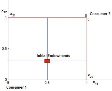
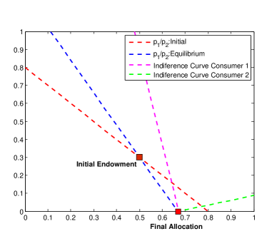
For this simple example, the reward sharing can be illustrated by using the Edgeworth box [23], shown in Fig. 1. The Edgeworth box is a rectangular diagram with consumer 1 and consumer 2 origins being located on bottom left and upper right corners, respectively. The width and height of the box show the total amount of commodities, here one. The bottom line is the $x$-axis for consumer 1 and the left side is the $y$-axis. For consumer 2, everything is flipped upside down and backward. Every point in the box represents a non-wasteful division of available commodities between the two consumers [26]. For instance, from Fig. 1, initial endowments read $(x_{11},x_{12})=(0.5,0.3)$ and $(x_{21},x_{22})=(0.5,0.7)$. Given the price vector $\mathbf{P}=(p_{1},p_{2})$, the budget line, i.e., the line with slope $p_{1}/p_{2}$ through the endowment point, divides the Edgeworth box into two budget sets $\mathcal{B}_{1}\left(\mathbf{P}\right)$ and $\mathcal{B}_{2}\left(\mathbf{P}\right)$. Then each consumer selects its demand so as to maximize its utility given the budget, by using the well-known indifference curves. When supply equals demand, market clears and equilibrium is reached. For the exemplary economy described before and for both initial and equilibrium prices, the budget lines are shown in Fig. 2. Moreover, by using indifference curves, convergence to equilibrium is illustrated. It can be seen that through the auction process, prices change; as a result, demands change until the convergence condition, i.e., market clearing, is satisfied. At equilibrium, $(x_{11},x_{12})=(0.67,0)$ and $(x_{21},x_{22})=(0.33,1)$. Note that in the presence of uncertainty, 1) commodities are state contingent and 2) expected utility functions are maximized; The overall procedure is however similar.

Figure 1: Edgeworth box, Example one.

Figure 2: Convergence to equilibrium, Example one.

V-A2 Example Two

In order to clarify the model and solution concept, in this section we consider an exchange economy consisting of two indivisible goods ($M=2$) and two consumers ($N=2$). We assume that the nature has two states ($S=2$). For consumer 1 and consumer 2, $\mathbf{a}_{1}=\left(0.2,0.8\right)$ and $\mathbf{a}_{2}=\left(0.5,0.5\right)$ denote, respectively, the probability vectors assigned to the set of possible states. Also, as before, we choose $\alpha=10^{-4}$. For states 1 and 2, utility matrices $\left[\mathbf{U}^{(i)}\right]_{N\times M}$, $i\in\{1,2\}$, are given as $\mathbf{U}^{(1)}=\begin{bmatrix}0.10&1.75\\ 2.20&2.20\end{bmatrix}$ and $\mathbf{U}^{(2)}=\begin{bmatrix}0.02&0.68\\ 0.96&0.96\end{bmatrix}$. Using $\mathbf{U}^{(i)}$ and $\mathbf{a}_{i}$, the expected utility functions $\bar{u}_{i}$, $i\in\{1,2\}$, yield

$$\bar{u}_{1}\left(\mathbf{X}_{1}\right)=0.02x^{(1)}_{11}+0.35x^{(1)}_{12}+0.016x^{(2)}_{11}+0.54x^{(2)}_{12},$$ (23)

and

$$\bar{u}_{2}\left(\mathbf{X}_{2}\right)=1.10x^{(1)}_{21}+1.10x^{(1)}_{22}+0.48x^{(2)}_{21}+0.48x^{(2)}_{22}.$$ (24)

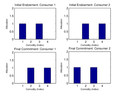
We assume that initial endowments are allocated randomly. Initial endowments and final allocations are shown in Figure 3. It can be seen that each consumer is assigned one good initially. Moreover, from the figure and also by (23) and (24), the Pareto optimal equilibrium is to allocate good 1 and good 2 respectively to consumer 2 and consumer 1, regardless of the occurred state. Note that in this specific example, contracts are identical for all states; this is however not the case in general. Relative prices are here $p^{(1)}_{1}/p^{(1)}_{2}=1$ and $p^{(2)}_{1}/p^{(2)}_{2}=1$.

Figure 3: Initial endowments and final commitments for Example two (indivisible goods). Indices are as follows: $1:x^{(1)}_{i1},2:x^{(1)}_{i2},3:x^{(2)}_{i1},4:x^{(2)}_{i2}$, where $i=1$ for consumer 1 and $i=2$ for consumer 2.

V-A3 Example Three

Our third example is similar to the second one, i.e., $M=2$, $N=2$, and $S=2$. Moreover, $\alpha=10^{-4}$. In this example, however, we assume that 1) goods are divisible, and 2) $\mathbf{a}_{1}=\left(0.8,0.2\right)$ and $\mathbf{a}_{2}=\left(0.5,0.5\right)$. Let $\mathbf{U}^{(1)}=\begin{bmatrix}1.25&2.12\\ 0.34&2.36\end{bmatrix}$ and $\mathbf{U}^{(2)}=\begin{bmatrix}2.55&1.55\\ 0.46&2.20\end{bmatrix}$. Then the expected utility functions $\bar{u}_{1}$ and $\bar{u}_{2}$ yield

$$\bar{u}_{1}\left(\mathbf{X}_{1}\right)=x^{(1)}_{11}+1.7x^{(1)}_{12}+0.31x^{(2)}_{11}+0.51x^{(2)}_{12},$$ (25)

and

$$\bar{u}_{2}\left(\mathbf{X}_{2}\right)=0.17x^{(1)}_{21}+1.18x^{(1)}_{22}+0.23x^{(2)}_{21}+1.10x^{(2)}_{22}.$$ (26)

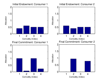
The initial endowments and final allocations are shown in Fig. 4.

Figure 4: Initial endowments and final commitments for Example three (divisible goods). Indices are as follows: $1:x^{(1)}_{i1},2:x^{(1)}_{i2},3:x^{(2)}_{i1},4:x^{(2)}_{i2}$, where $i=1$ for consumer 1 and $i=2$ for consumer 2.

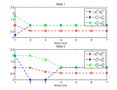
For both states, relative prices and relative demands of goods are shown in Fig. 5. It can be seen that the prices of goods in excess demand increase, yielding the demands to decrease. As a result, the demands of other goods either do not change or increase, since goods are gross substitutes. The process continues until market clears; that is, a price vector is reached in which demand equals supply.

Figure 5: Relative prices and aggregate demands, Example three.

V-B Performance Evaluation

In this section, we consider a network with ten users ($M=10$) and four SBSs ($N=4$). The average channel gain matrix between SBSs and users, $\left[\mathbf{H}\right]_{N\times M}$, is given as

$\mathbf{H^{{}^{\circ\frac{1}{2}}}}=10^{-2}\times\begin{bmatrix}10&71&8&99&99&99&49&99&21&89\\ 11&91&96&95&89&9&21&37&17&30\\ 1&9&92&91&96&11&52&88&52&18\\ 99&19&4&89&92&91&39&7&61&14\end{bmatrix}$.

The components of $\mathbf{H}$ are selected randomly. As conventional, we assume that the matrix $\mathbf{H}$ can be written as $\mathbf{H}=\mathbf{F}{\circ}\mathbf{G}$, where $\mathbf{F}$ and $\mathbf{G}$ are average fading gain and path-loss matrices. We let

$\mathbf{F^{{}^{\circ\frac{1}{2}}}}=10^{-2}\times\begin{bmatrix}10&19&50&21&9&29&4&9&25&8\\ 41&88&32&45&90&9&19&21&8&12\\ 5&6&1&93&98&9&24&40&15&5\\ 50&15&18&92&97&89&8&7&1&2\end{bmatrix}$.

According to our system model, initially we assume that every SBS $i$ knows only $\mathbf{H}_{i}$; that is, each SBS has only local statistical CSI. The antenna gain is initially $G=3$. Noise plus interference power is normalized to one. We assume that the nature accepts one of the four possible states; that is, $\mathcal{S}=\left\{s_{1},s_{2},s_{3},s_{4}\right\}$, where $s_{1}=\left\{2,2,2,2\right\}$, $s_{2}=\left\{6,2,1,5\right\}$, $s_{3}=\left\{3,2,4,7\right\}$, and $s_{4}=\left\{1,3,2,5\right\}$. In $s_{i}$, $i\in\left\{1,2,3,4\right\}$, the $j$-th component is the energy level of SBS $j$ at state $i$. The probability distributions assigned to nature’s states by SBSs are as follows: $\mathbf{a}_{1}=\left(0.10,0.50,0.20,0.20\right)$, $\mathbf{a}_{2}=\left(0.25,0.25,0.10,0.40\right)$, $\mathbf{a}_{3}=\left(0.35,0.15,0.10,0.40\right)$, and $\mathbf{a}_{4}=\left(0.20,0.30,0.30,0.20\right)$. These probability distributions are selected uniformly randomly from the 4-dimensional probability space. Moreover, we choose $\alpha=10^{-4}$. It is clear that four sets of energy levels (nature’s states) and ten users (commodities) result in 40 state contingent commodities. Each SBS (consumer) determines its demand so as to maximize its expected average utility, as discussed in Section III and also by simple examples in Section V-A2. For evaluations, we consider the following scenarios:

• Maximum Received Power Assignment (MRP): In this scenario, user association is performed by a central unit given average channel gain matrix, $\mathbf{H}$. By means of exhaustive search, every user is assigned to the SBS to which it has the maximum average channel gain. Assignment based on received power has been widely used to solve the user association problem (e.g., in [33]).

• Nearest SBS Assignment (NSBS): In this scenario, user association is performed by a central unit given geographical location of users and SBSs, as well as the path-loss exponent. In our model, the path-loss matrix $\mathbf{G}$ follows by element-wise division of $\mathbf{H}$ into $\mathbf{F}$. We assume that the path-loss exponent is equal for all links; thus larger distance yields larger path loss and vice versa. By means of exhaustive search, every user is assigned to the SBS to which it has the minimum path-loss. It is clear that the performance of MRP method serves as an upper-bound for that of NSBS. Distance-based assignment is a conventional method to solve different types of association problems (e.g., in [34]).

• Maximum Weighted Matching Assignment (MWM): Given the average channel matrix $\mathbf{H}$, the user association problem is cast as a maximum-weighted matching problem. More precisely, we construct a bipartite graph, with one party being the users and the other party being the SBSs. The weight of each edge connecting an SBS to a user is the average channel gain. The Hungarian algorithm [35] is used to assign users to SBSs in a way that each user is associated to only one SBS. Matching theory has been widely used to solve the resource allocation as well as association problems (e.g., in [36]).

• Auction Assignment (AUC): In this scenario, our proposed model and algorithm is used for distributed user association under uncertainty.

• Random Assignment (RND): Users are associated randomly.

It should be also mentioned that many user association methods cannot be directly compared to each other. This is because, as discussed in Section I and also summarized in Table I, every method is designed for a specific system model and aims at optimizing a particular performance metric.

In the next step, the MRP, AUC, and RND association methods are used in conjunction with the three transmission scenarios described in Section II.

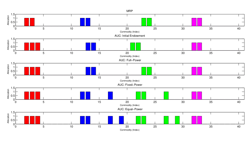
For SBS 1, the allocation by MRP, as well as initial endowments and allocations by using the auction process for different transmission models are shown in Fig. 6. Note that the MRP allocation is based on average channel gain only, hence does not depend on the state and/or transmission model. The results are similar for other SBSs.

Figure 6: Initial endowments and final commitments. Indices $1,2,...,39,40$ correspond to $x_{i1}^{(1)},x_{i2}^{(1)},...,x_{i9}^{(4)},x_{i10}^{(4)}$, with $i=1$ representing SBS 1.

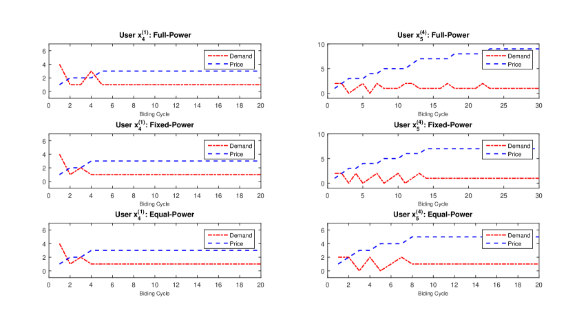
For AUC and for two exemplary state contingent commodities (User 4 at State 1, $x_{4}^{(1)}$, and User 5 at State 4, $x_{5}^{(4)}$), variations in prices and aggregate demands are depicted in Fig. 7, as a function of auctions’ iterations (biding cycles), for different transmission models. As expected, excess demand results in price growth. The curves for the rest of state contingent commodities are similar.

Figure 7: Variations in prices and aggregate demands for two exemplary state contingent commodities.

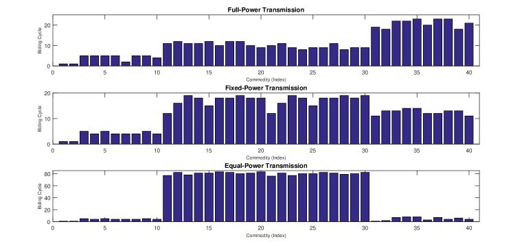
The required number of iterations for the price and demand of each good to converge, or, in other words, the required number of biding cycles for three (out of four) SBSs to leave the auction, is depicted in Fig. 8. As discussed in Section IV-A, the convergence time depends on initial endowments and utilities, and cannot be described by a general formula.

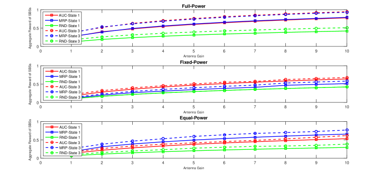
The performance of the proposed model and solution in terms of aggregate network utility is illustrated in Fig. 9, for State 1 and State 3. The curves for the other two states follow similar paths.

Figure 8: Required number of biding cycles to converge for each state contingent commodity. Indices $1,2,...,39,40$ correspond to $x_{1}^{(1)},x_{2}^{(1)},...,x_{9}^{(4)},x_{10}^{(4)}$.

Figure 9: Performance of auction model under uncertainty. Aggregate rewards are normalized.

Finally, in Fig. 10, we show the performance of the AUC assignment approach in comparison with other methods described before, i.e., MRP, NSBS, MWM and RND. As exemplary states, we consider State 3 and State 4 in conjunction with fixed-power transmission scenario.

Figure 10: Performance of the proposed approach compared to some other user association methods. Aggregate rewards are normalized.

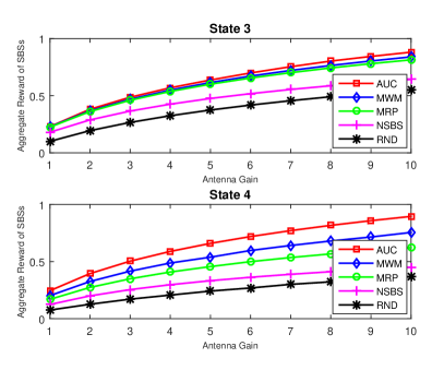
From Fig. 9 and Fig. 10, it can be concluded that the auction model performs well. Moreover, as expected, the performance gain of the auction model depends on the transmission model and also varies in different state. The best performance appears in fixed-power transmission, where some users might not be served as the result of lack of energy. Note that in any case the approach requires little information, yield equilibrium, and is implementable in a distributed manner. The occasional small inefficiency is mainly due to the uncertainty, as described in the following:

• In the auction process, SBSs are assigned initial endowments, thereby a budget. As a result, they can select only a specific number of users, depending on the initial endowments. Initial endowments, however, are granted simply at random, leading to an inefficiency in using the harvested energy. Nonetheless, if some information is available at the MBS, for instance some sample data from the past, initial endowments can be granted in a more efficient way, so that an SBS with (possibly) larger harvested energy receives larger budget. Using this policy, the performance of the auction process would be dramatically improved.

• In the auction process, optimization is performed based on expected utility functions, which, by (9), depends on probability distributions assigned to the set of states by the SBSs. In the auction model, in general, these distributions are considered to be simply the uniform distribution. However, similar to the previous argument, this assumption yields inefficiency, since it might yield the expected utility functions to be different from true ones. Therefore, a smarter choice is to select a distribution based on past sample data, and/or by using some forecasting procedure to reduce the effect of uncertainty, so that the expected utility functions are similar to true ones.

VI Conclusion

We have considered the user association problem in small cell networks, where each small cell obtains its energy by using its local energy harvesting units. Desired is to develop a distributed user association scheme that is able to cope with the uncertainty hidden in the problem, caused by the opportunistic nature of energy harvesting. We have modeled the small cell network as a competitive market, and the user association as an exchange economy with uncertainty. In our setting, we established the existence of Arrow-Debreu equilibrium, and investigated its characteristics such as uniqueness and optimality. We have used the Walras’ tatonnement procedure, combined with the static knapsack problem, to implement equilibrium prices efficiently.

References

- [1] E. Hossain, M. Rasti, H. Tabassum, and A. Abdelnasser, “Evolution toward 5G multi-tier cellular wireless networks: An interference management perspective,” IEEE Wireless Communications, vol. 21, no. 3, pp. 118–127, June 2014.
- [2] G. Fodor, E. Dahlman, G. Mildh, S. Parkvall, N. Reider, G. Miklós, and Z. Turányi, “Design aspects of network assisted device-to-device communications,” IEEE Communications Magazine, vol. 50, no. 3, pp. 170–177, March 2012.
- [3] K.J. Zou, K.W. Yang, M. Wang, B. Ren, J. Hu, J. Zhang, M. Hua, and X. You, “Network synchronization for dense small cell networks,” IEEE Wireless Communications, vol. 22, no. 2, pp. 108–117, April 2015.
- [4] R. Amin and J. Martin, “Assessing performance gains through global resource control of heterogeneous wireless networks,” IEEE Transactions on Mobile Computing, vol. PP, no. 99, pp. 1–1, 2015.
- [5] H. Zhang, Y. Wang, and H. Ji, “Resource optimization based interference management for hybrid self-organized small cell network,” IEEE Transactions on Vehicular Technology, vol. PP, no. 99, pp. 1–1, 2015.
- [6] H. Zhang, C. Jiang, and J. Cheng, “Cooperative interference mitigation and handover management for heterogeneous cloud small cell networks,” IEEE Wireless Communications, vol. 22, no. 3, pp. 92–99, June 2015.
- [7] N. N. Namvar, W. Saad, B. Maham, and S. Valentin, “A context-aware matching game for user association in wireless small cell networks,” in IEEE International Conference on Acoustics, Speech and Signal Processing, May 2014, pp. 439–443.
- [8] O. Semiari, W. Saad, S. Valentin, M. Bennis, and B. Maham, “Matching theory for priority-based cell association in the downlink of wireless small cell networks,” in IEEE International Conference on Acoustics, Speech and Signal Processing, May 2014, pp. 444–448.
- [9] W. Saad, Z. Han, R. Zheng, M. Debbah, and H.V. Poor, “A college admissions game for uplink user association in wireless small cell networks,” in Proceedings IEEE INFOCOM, April 2014, pp. 1096–1104.
- [10] Y. Chen, J. Li, W. Chen, Z. Lin, and B. Vucetic, “Joint user association and resource allocation in the downlink of heterogeneous networks,” IEEE Transactions on Vehicular Technology, vol. PP, no. 99, pp. 1–1, 2015.
- [11] A. Mesodiakaki, F. Adelantado, L. Alonso, and C. Verikoukis, “Energy-efficient user association in cognitive heterogeneous networks,” IEEE Communications Magazine, vol. 52, no. 7, pp. 22–29, July 2014.
- [12] S.O. Elbassiouny, A. Elhamy, and A.S. Ibrahim, “Traffic-aware user association technique for dynamic on/off switching of small cells,” in IEEE Wireless Communications and Networking Conference, March 2015, pp. 866–871.
- [13] G. Athanasiou, T. Korakis, O. Ercetin, and L. Tassiulas, “A cross-layer framework for association control in wireless mesh networks,” IEEE Transactions on Mobile Computing, vol. 8, no. 1, pp. 65–80, Jan 2009.
- [14] Q. Ye, B. Rong, Y. Chen, M. Al-Shalash, C. Caramanis, and J.G. Andrews, “User association for load balancing in heterogeneous cellular networks,” IEEE Transactions on Wireless Communications, vol. 12, no. 6, pp. 2706–2716, June 2013.
- [15] A. H. Sakr and E. Hossain, “Analysis of k-tier uplink cellular networks with ambient RF energy harvesting,” IEEE Journal on Selected Areas in Communications, vol. PP, no. 99, pp. 1–1, 2015.
- [16] S. Sudevalayam and P. Kulkarni, “Energy harvesting sensor nodes: Survey and implications,” IEEE Communications Surveys Tutorials, vol. 13, no. 3, pp. 443–461, March 2011.
- [17] Y. Song, M. Zhao, W. Zhou, and H. Han, “Throughput-optimal user association in energy harvesting relay-assisted cellular networks,” in International Conference on Wireless Communications and Signal Processing, Oct 2014, pp. 1–6.
- [18] P.-S. Yu, J. Lee, T.Q.S. Quek, and Y.-W.P. Hong, “Energy harvesting personal cells-traffic offloading and network throughput,” in IEEE International Conference on Communications, June 2015, pp. 2184–2189.
- [19] D. Liu, Y. Chen, K.-K. Chai, T. Zhang, and C. Pan, “Adaptive user association in hetnets with renewable energy powered base stations,” in International Conference on Telecommunications, May 2014, pp. 93–97.
- [20] H. Xu, T. Zhang, Z. Zeng, and D. Liu, “Distributed user association for delay-load tradeoffs in energy harvesting enabled hetnets,” in IEEE Wireless Communications and Networking Conference Workshops, March 2015, pp. 386–390.
- [21] D. Liu, Y. Chen, K.-K. Chai, and T. Zhang, “Two dimensional optimization on user association and green energy allocation for hetnets with hybrid energy sources,” IEEE Transactions on Communications, vol. PP, no. 99, pp. 1–1, 2015.
- [22] J. Rubio, A. Pascual-Iserte, J. del Olmo, and J. Vidal, “User association for load balancing in heterogeneous networks powered with energy harvesting sources,” in Globecom Workshops, Dec 2014, pp. 1248–1253.
- [23] A. Mas-Colell, M. D. Whinston, and J. R. Green, Microeconomic Theory, Oxford University Press, 1985.
- [24] G. Debreu, Theory of Value: An Axiomatic Analysis of Economic Equilibrium, Yale University Press, 1987.
- [25] F. Gul and E. Stacchetti, “Walrasian Equilibrium with Gross Substitutes,” Journal of Economic Theory, vol. 87, no. 1, pp. 95–124, July 1999.
- [26] J. Levin, “General equilibrium,” Availabl online at: http://www.stanford.edu/ jdlevin/Econ%20202/General%20Equilibrium.pdf, 2006.
- [27] H. Uzawa, “Walras’ t tonnement in the theory of exchange,” The Review of Economic Studies, vol. 27, no. 3, pp. 182–194, June 1960.
- [28] R. Mochaourab, B. Holfeld, and T. Wirth, “Distributed channel assignment in cognitive radio networks: Stable matching and walrasian equilibrium,” IEEE Transactions on Wireless Communications, vol. 14, no. 7, pp. 3924–3936, July 2015.
- [29] N. Nisan, T. Roughgarden, E. Tardos, and V.V. Vazirani, Algorithmic Game Theory, Cambridge University Press, New York, NY, USA, 2007.
- [30] J. Q. Cheng and M. P. Wellman, “The WALRAS algorithm: A convergent distributed implementation of general equilibrium outcomes,” Computational Economics, vol. 12, no. 1, pp. 1–24, 1998.
- [31] R. Axtell, “The complexity of exchange,” The Economic Journal, vol. 115, pp. F193–F210, 2005.
- [32] S. Martello and P. Toth, Knapsack Problems: Algorithms and Computer Implementations, John Wiley & Sons, Inc., 1990.
- [33] Y. Lin, W. Bao, W. Yu, and B. Liang, “Optimizing user association and spectrum allocation in hetnets: A utility perspective,” IEEE Journal on Selected Areas in Communications, vol. 33, no. 6, pp. 1025–1039, June 2015.
- [34] K. Son, H. Kim, Y. Yi, and B. Krishnamachari, “Base station operation and user association mechanisms for energy-delay tradeoffs in green cellular networks,” IEEE Journal on Selected Areas in Communications, vol. 29, no. 8, pp. 1525–1536, September 2011.
- [35] H.W. Kuhn, “The Hungarian method for the assignment problem,” Naval Research Logistic Quarterly, vol. 2, no. 1, pp. 83–97, 1955.
- [36] S. Maghsudi and S. Stanczak, “Joint power allocation and relay selection for network-coded two-way relaying,” in Annual Conference on Information Sciences and Systems, March 2012, pp. 1–6.