Local equilibrium in bird flocks

Abstract

The correlated motion of flocks is an instance of global order emerging from local interactions. An essential difference with analogous ferromagnetic systems is that flocks are active: animals move relative to each other, dynamically rearranging their interaction network. The effect of this off-equilibrium element is well studied theoretically, but its impact on actual biological groups deserves more experimental attention. Here, we introduce a novel dynamical inference technique, based on the principle of maximum entropy, which accodomates network rearrangements and overcomes the problem of slow experimental sampling rates. We use this method to infer the strength and range of alignment forces from data of starling flocks. We find that local bird alignment happens on a much faster timescale than neighbour rearrangement. Accordingly, equilibrium inference, which assumes a fixed interaction network, gives results consistent with dynamical inference. We conclude that bird orientations are in a state of local quasi-equilibrium over the interaction length scale, providing firm ground for the applicability of statistical physics in certain active systems.

Animal groups moving in concert such as mammal herds, fish schools, and bird flocks show that in biology, just as in physics, local coordination can result in large-scale order Camazine2001 ; krause2002 ; sumpter2010 . However flocks differ from classical statistical physics in that their constituents are active: they constantly move by self-propulsion, pumping energy into the system and keeping it out of equilibrium Toner1998 ; Review ; vicsek2012 ; marchetti2013 . The key element is the rearrangement of the interaction network due to the active motion of individuals relative to each other, continuously changing their neighbours. Theoretical studies show that network rearrangement has major consequences, which include enhancing collective order, reducing from 3 to 2 the lower critical dimension, and affecting the critical exponents Toner1995 ; Toner1998 .

However, the importance of activity must be assessed with respect to the relevant time scales of the system. The impact of network rearrangement depends on the interplay between its characteristic time scale, $\tau_{\rm network}$, defined as the average time it takes an individual to change its interaction neighbours, and the local relaxation time scale, $\tau_{\rm relax}$, defined as the time needed to relax locally the order parameter if the interaction network were fixed. If $\tau_{\rm network}\leq\tau_{\rm relax}$, the interaction network rearranges at least as fast as the order parameter relaxes, and the system remains far from equilibrium. If on the other hand $\tau_{\rm relax}\ll\tau_{\rm network}$, the relaxation of the order parameter is adiabatic, closely following the network as it slowly evolves. In this case, even though the system behaves in an out-of-equilibrium manner on the longest scales, it locally obeys a condition of equilibrium, and we expect some of the tools of equilibrium statistical physics to be applicable.

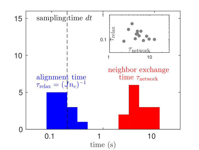
Here, we explicitly address the impact of network activity by developing a new inference method based on the exact integration of maximum-entropy dynamical equations, thus accounting for the reshuffling of the network. We apply the method to data of starling flocks of up to 600 individuals Ballerini2008a ; Cavagna2008b ; Cavagna2008a ; Attanasi2015 (see Materials and Methods and Table S1 for data summary), inferring the relevant parameters of the interactions between individuals. We find that the alignment relaxation time, $\tau_{\rm relax}$, is more than one order of magnitude shorter than the network rearrangement time, $\tau_{\rm network}$. Consistently, we show that the parameters learned from the dynamics are consistent with those obtained by an equilibrium-like inference, which assumes a fixed network Bialek2012 . Our results suggest that natural flocks are in a state of local quasi-equilibrium over the interaction length scale, meaning that the relatively slow rearrangement of the local interaction network does not affect the ordering dynamics up to certain scales.

Figure 1: Performance of the inference methods on the predicted interaction range $n_{c}$. A. Inferred versus real $n_{c}$ obtained by applying our new inference method to simulated data generated with Eq. 1 at various interaction ranges. The method performs well for different values of the sampling rate $dt$. B. Dependence of the inferred $n_{c}$ on the sampling time $dt$. On simulated data with $n_{c}=10$ (dashed line), the inference method based on exact integration (red points) performs well regardless of the sampling time $dt$. By contrast, the inference method based on Euler’s integration method (green points) overestimates the true interaction range at large $dt$. C. A similar trend is observed when we apply the two inference procedures to real flocking data, as illustrated here on one flocking event. Note that in this case the true value is not known. Error bars represent standard errors over time frames.

To compare the relevant time scales of the ordering process in flocks, we first need to learn the dynamical rules of their behaviour. Learning these rules usually relies on inferring the parameter of a chosen model directly from the data, as has been recently done in surf scoters Lukeman:2010p9518 , prawns mann2012 and fish schools Katz2011a ; Herbert-Read2011 ; Gautrais2012 ; strandburg2013 ; Rosenthal2015 . Although in these studies the local rules of interaction were often learned using small groups, in some cases they could also be used to predict large-group behavior Gautrais2012 ; Rosenthal2015 . Here, instead of assuming a model a priori, we apply the principle of maximum entropy to the trajectories of all birds in the group Cavagna2013 . We look for a distribution of the stochastic process that is as random as possible, while agreeing with the data on a key set of experimental observables.

In a flock of size $N$, we call $\vec{s}_{i}(t)$ the three-dimensional flight orientation of bird $i$ at time $t$. The maximum entropy distribution over possible flock trajectories that is consistent with the correlation functions $\langle\vec{s}_{i}(t)\cdot\vec{s}_{j}(t)\rangle$, as well as their derivatives $\langle d\vec{s}_{i}(t)/dt\cdot\vec{s}_{j}(t)\rangle$, can be exactly mapped, in the limit of strong polarization $P\equiv(1/N)\|\sum_{i}\vec{s}_{i}\|\approx 1$, onto the following stochastic differential equation (see SI and Ref. Cavagna2013 ):

$$\frac{d\vec{s}_{i}}{dt}=\left(\sum_{j}J_{ij}\vec{s}_{j}+\vec{\xi}_{i}\right)_{\perp},$$ (1)

where $\vec{\xi}_{i}$ is a random white noise, and where the projection $\vec{x}_{\perp}\equiv\vec{x}-\vec{s}_{i}(\vec{x}\cdot\vec{s}_{i})$ onto the plane perpendicular to $\vec{s}_{i}$ ensures that $\vec{s}_{i}$ remains of norm 1. Equation (1) can be viewed as a generalization of the Vicsek model Vicsek1995 : each bird modifies its flight direction according to a weighted average of the directions of its neighbours. The interaction matrix $J_{ij}$ encodes how much bird $i$ is influenced by (i.e. interacts with) bird $j$. Given the experimentally measured correlation functions, entropy maximization yields equations that fix the values of the noise amplitude and the interaction matrix $J_{ij}$. This matrix has too many parameters to be reliably determined from the data, but we can reduce its complexity by parametrising it. It was shown in Cavagna2015a that the interaction decays exponentially with the topological distance $k_{ij}$ between birds,

$$J_{ij}=J\exp(-k_{ij}/n_{c})\ ,$$ (2)

where $k_{ij}$ denotes the (time-dependent) rank of bird $j$ among the neighbours of bird $i$ ranked by distance. This interaction matrix has just two parameters: $n_{c}$ is the topological interaction range, while $J$ is the overall strength of the interaction. The noise is uncorrelated among birds and of uniform magnitude $T$, by analogy with physical temperature: $\langle\vec{\xi}_{i}(t)\cdot\vec{\xi}_{j}(t^{\prime})\rangle=2\,d\,T\,\delta_{ij}\delta(t-t^{\prime})$, where $d$ is the space dimension ($d=3$ in the following).

In principle, to learn the parameters of Eq. 1 one needs actual continuous-time derivatives. In practice, we only have configurations separated by the finite experimental sampling time $dt$. A common solution is to use Euler’s approximation:

$$\vec{s}_{i}(t+dt)\approx\vec{s}_{i}(t)+dt\,\sum_{j}J_{ij}\vec{s_{j}}_{\perp}+\sqrt{2Tdt}\,\vec{\eta_{i}}_{\perp},$$ (3)

where $\vec{\eta}_{i}$ is a normally distributed vector of variance 1 in each direction. The conditional likelihood of the data given the model, $P[\{\vec{s}_{i}(t+dt)\}|\{\vec{s}_{i}(t)\}]$, can be written in Gaussian form after expanding Eq. (3) in the spin-wave approximation (see Materials and Methods). Maximising this likelihood yields values for the alignment parameters $n_{c}$, $J$ and $T$ (see Ref. Cavagna2013 and SI).

Euler’s approximation is used by virtually all methods that try to fit a dynamical equation to a discrete time series Katz2011a ; Herbert-Read2011 ; Gautrais2012 . However, it is inappropriate when the experimental sampling time, $dt$, is larger than the intrinsic relaxation timescale, $\tau_{\rm relax}$. In this case information spreads between subsequent frames beyond the directly interacting neighbours and Euler’s approximation overestimates the range of the interaction, as we shall see below. To overcome this issue, we rewrite Eq. 1 by formally subtracting $\sum_{l}J_{il}\vec{s_{i}}_{\perp}=0$ from it:

$$\frac{d\vec{\bf s}}{dt}=-J{\bm{\Lambda}}\vec{\bf s}_{\perp}+\vec{\bm{\xi}}_{\perp}.$$ (4)

Bold symbols denote vectors and matrices over bird indices; the matrix $\Lambda_{ij}\equiv\delta_{ij}\sum_{l}n_{il}-n_{ij}$, where $n_{ij}=e^{-k_{ij}/n_{c}}$ is the connectivity matrix (2). ${\bm{\Lambda}}$ is analogous to a Laplacian defined on a lattice, and obeys the sum rule: $\sum_{j}\Lambda_{ij}=0$. In the spin-wave approximation, where all orientations $\vec{s}_{i}$ point in almost the same direction, this relation ensures that ${\bm{\Lambda}}\vec{\bf s}$ has almost no contribution along the common direction of flight, implying $({\bm{\Lambda}}\vec{\bf s})_{\perp}\approx{\bm{\Lambda}}\vec{\bf s}$ (see Materials and Methods and SI). Equation 4 is now linear and it can be integrated exactly:

$$\vec{\bf s}(t+dt)=e^{-J{\bm{\Lambda}}dt}\vec{\bf s}(t)+\int_{0}^{dt}du\,e^{-J{\bm{\Lambda}}(dt-u)}\vec{\bm{\xi}}_{\perp}(t+u)\ .$$ (5)

This result assumes a constant $J_{ij}$ in the interval $dt$, which is a good approximation if $dt\ll\tau_{\rm network}$. Fortunately, this same condition is necessary for the very possibility to collect data: tracking requires to follow each individual across time, which is only possible if individuals do not significantly change their neighbourhood between consecutive frames. The integrated noise in the right-hand side of (5) is Gaussian, of mean zero and covariance $4T\int_{0}^{dt}du\,e^{-J{\bm{\Lambda}}u}e^{-J{\bm{\Lambda}}^{\dagger}u}$. Using the exact solution (5) we can write an explicit expression for the (Gaussian) conditional likelihood $P[\{\vec{s}_{i}(t+dt)\}|\{\vec{s}_{i}(t)\}]$, which can then be maximised over the parameters of the model (see Materials and Methods).

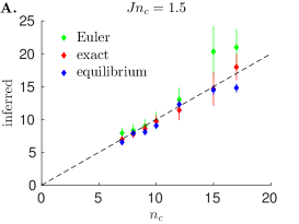
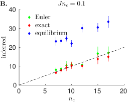
We first tested our dynamical inference method on synthetic data simulated using the model of Eq. 1, with $\tau_{\mathrm{relax}}\approx 0.7$, for various values of the interaction range $n_{c}$ (see Materials and Methods). We infer the parameters of the model using either Euler’s rule or the result of exact integration, for different values of the sampling time ranging from $dt=0.2$ to $dt=0.8$. The method based on exact integration predicts the interaction range $n_{c}$ well, regardless of $dt$ (Fig. 1A and B), while the method based on Euler’s approximation largely overestimates $n_{c}$ at large $dt$ (Fig. 1B). We can now apply our dynamical inference to real flocks and learn the model parameters. First, we used data of natural flocks to check the effect of changing the sampling time $dt$, from the real sampling time of our setup, $dt=0.2$ s (see Materials and Methods), to $0.8$ s. Although we cannot compare the inferred value of $n_{c}$ to the ground truth as in simulations, we observe a similar trend as a function of $dt$ (Fig. 1C), with the exact integration and Euler’s approximation methods agreeing only at small $dt$. This suggests that the sampling time of $0.2$ s is of the same order as the orientation relaxation time $\tau_{\rm relax}$, as we will confirm below. It also indicates that the inference method based on exact integration is extracting the parameters of alignment reliably.

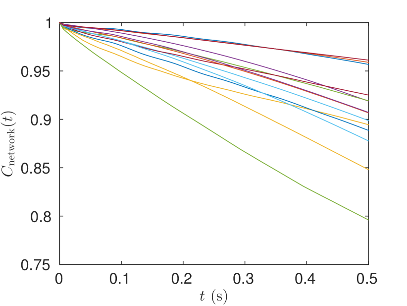
Using the model parameters learned from the data, we evaluate the two time scales of interest for activity, namely relaxation of the orientations and network rearrangement. We estimated the network rearrangement time $\tau_{\rm network}$ experimentally for each flocking event as the characteristic decay time of its autocorrelation function $C_{\rm network}(t)=\sum_{ij}n_{ij}(t_{0})n_{ij}(t_{0}+t)$, by fitting $C_{\rm network}(t)\approx C_{0}\exp(-t/\tau_{\rm network})$ (Fig. S1).

Working out the time scale of relaxation is more subtle. The relevant quantity is the product of the interaction strength $J$, which has units of inverse time, by the dimensionless connectivity matrix, $\bm{\Lambda}$, as can be seen from Eq. (4). Since there are $n_{c}$ neighbours acting on each individual, the total alignment force is of order $Jn_{c}$, suggesting that the characteristic time scale of relaxation of the orientations is $\tau_{\rm relax}\sim(Jn_{c})^{-1}$. This result, however, seems at odds with the well-known fact that systems with spontaneously broken continuous symmetry - such as flocks - have correlation length and relaxation time that diverge with the system size $L$ (Goldstone theorem Parisi ). On the other hand, we do not expect the large-scale modes responsible for this divergence to affect the local relaxation dynamics and its interplay with network reshuffling. To clarify this issue we calculate the dynamical autocorrelation function of the fluctuations of the order parameter, $C_{\mathrm{relax}}(t)=\langle\delta\vec{s}_{i}(t_{0})\cdot\delta\vec{s}_{i}(t_{0}+t)\rangle$, where $\delta\vec{s}_{i}=\vec{s}_{i}-\langle\vec{s}_{i}\rangle$. We consider a fixed lattice, because we need to gauge relaxation in absence of network rearrangements, resulting in the autocorrelation function (see SI):

$$C_{\mathrm{relax}}(t)=\int_{1/L}^{1/a}d^{d}k\ \frac{e^{-Ja^{2}n_{c}\,k^{2}t}}{Ja^{2}n_{c}\,k^{2}}\ ,$$ (6)

where $a$ is the lattice spacing. The infrared divergence at small $k$, which correspond to large-scale modes, makes the integral divergent in the $L\to\infty$ limit for $d=2$ (Mermin-Wagner theorem Mermin ). In $d=3$ the integral is finite, but the correlation function is a power law, so that the relaxation time diverges with $L$ (Goldstone theorem). The small $k$ modes in (6) correspond to long wavelengths fluctuations spanning the entire flock, causing the local order parameter to relax slowly. However, these long wavelength fluctuations do not contribute to the disordering of the local interaction network: if the wavelength of a fluctuation is much larger than the interaction range, all directions of motion in the interaction neighbourhood fluctuate in unison, causing no change in the mutual positions of the birds. We conclude that the autocorrelation function that impacts on local network rearrangements only includes contributions from wavelengths up to the local interaction range (let us call it $r_{c}$). This amounts to restricting the integral in (6) to the modes $r_{c}^{-1}\leq k\leq a^{-1}$, thus eliminating the infrared divergent modes $k\sim 1/L$. The resulting correlation function is exponentially decaying (see SI for the calculation of the integral), with finite relaxation time equal to $\tau_{\mathrm{relax}}=(Jn_{c})^{-1}$, consistent with our initial guess. We note that, by considering wavelengths up to the interaction range, we are still dealing with a coarse-grained field theory, as in most biological systems the scale of interaction extends over tens of neighbours.

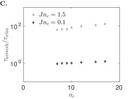
We can now proceed with the comparison of $\tau_{\rm network}$ and $\tau_{\rm relax}$. Results are summarised in Fig. 2. The two time scales clearly separate, with local relaxation almost two orders of magnitude faster than network reshuffling. This separation of time scales suggests that flocks are in a state of local equilibrium. The network of interactions changes slowly enough for the dynamics of flight orientations to catch up before neighbours reshuffle. In other words, the orientation dynamics tracks network changes adiabatically. Note that this statement holds only locally, at the scale of the interaction range, as both $\tau_{\rm network}$ and $\tau_{\rm relax}$ are defined on that scale.

Figure 2: Comparison between the two relevant time scales of active matter, as inferred in 14 natural flocks using our inference method based on exact integration. Histograms of the neighbour exchange time $\tau_{\rm network}$ versus the local alignment time $\tau_{\rm relax}=1/Jn_{c}$, show that the relaxation of orientations is much faster than the turnover of neighbours. Note that the experimental sampling time $dt=0.2$ s (dashed line) is of the same order as the alignment time, justifying the use of exact integration. Inset: the scatter plot of $\tau_{\rm relax}$ versus $\tau_{\rm network}$ shows no correlation between the two quantities.

Since flocks behave as if they were in local equilibrium, an equilibrium inference procedure, which takes as input the local spatial correlation computed from a snapshot of the birds’ flight orientation Bialek2012 , should be consistent with the results of the dynamical inference. To check this prediction, we recall the equilibrium-like inference method of Bialek2012 . For symmetric $J_{ij}$, Eq. 1 is the Langevin equation derived from the Hamiltonian of the Heisenberg model

$$\mathcal{H}=-\frac{1}{2}\sum_{i,j}J_{ij}\vec{s}_{i}\cdot\vec{s}_{j}.$$ (7)

When $J_{ij}$ varies slowly in time, the fluctuations of $\vec{s}_{i}$ are in quasi-equilibrium and distributed according to Boltzmann’s law:

$$P(\vec{s}_{1},\ldots,\vec{s}_{N})\sim\exp\left(-{\mathcal{H}}/{T}\right).$$ (8)

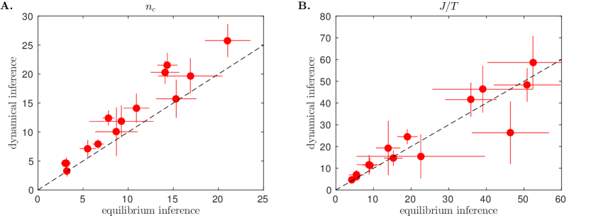
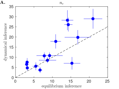
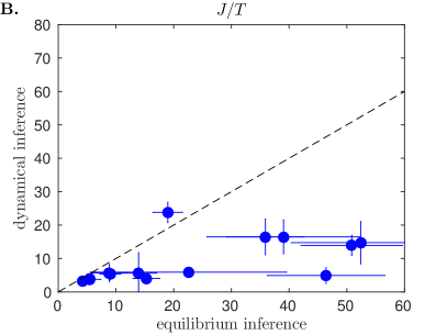
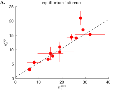
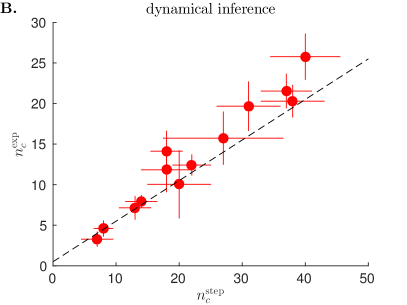
We recognise the maximum entropy distribution consistent with the local correlation index $\sum_{ij}n_{ij}\langle\vec{s}_{i}\vec{s}_{j}\rangle$ fitted in Ref. Bialek2012 . In practice, the equilibrium inference consists in maximising the likelihood of Eq. 8 over its parameters $n_{c}$ and $J/T$ (see Materials and Methods and SI). If the variations of $n_{ij}$ are slow compared to the dynamics of $\vec{s}_{i}$, $\tau_{\rm network}\gg\tau_{\rm relax}$, this inference procedure should give an accurate estimate of the alignment parameters. If however the two time scales are comparable, we expect the equilibrium inference to overestimate the true $n_{c}$, as the frequent exchange of neighbours results in an effective number of interaction partners that is larger than the instantaneous one. We verified both these expectations on simulated data, by showing that the equilibrium inference is accurate for $\tau_{\rm network}\sim 100\tau_{\rm relax}$, but overestimates $n_{c}$ for $\tau_{\rm network}\sim\tau_{\rm relax}$ (see Fig. S2). When applied to empirical data, the dynamical and equilibrium inferences give consistent results, and predict the same interaction range, $n_{c}$, and coupling-to-noise ratio, $J/T$ (Fig. 3) Note that, while the dynamical inference provides the strength of the interaction, $J$, and the strength of the noise, $T$, separately, the equilibrium inference only gives the ratio $J/T$, which is the quantity to compare. To better appreciate this result, recall that the two inference procedures are based on independent pieces of information: the equilibrium inference uses instantaneous orientations, while the dynamical inference exploits how these orientations change in time. Their agreement confirms that the alignment dynamics of flocks are in an effective state of equilibrium over the range $n_{c}$.

Figure 3: Inference on natural flocks. For each of the 14 flocking events, the parameters of the model were inferred using either the dynamical inference method presented here, with $dt=0.2$ s, or an equilibrium inference method as in Bialek2012 . A. Both methods agree well on the predicted value of the alignment range $n_{c}$. B. While the dynamical method infers the alignment strength $J$ and the noise amplitude $T$ separately, the equilibrium method only infers their ratio $J/T$, the value of which is consistent between the two methods. Error bars represent standard errors over time frames.

Theoretical studies of active matter indicate that out-of-equilibrium effects induced by the rearrangement of the interaction network play a major role in the ordering of the system Toner1998 ; Review . In this light, any attempt to understand the properties of active biological systems based on equilibrium approaches may seem inappropriate. Does it mean that we should we always relinquish the methods of equilibrium statistical mechanics when dealing with active systems? Our results address this question by showing that bird flocks are in a state of local equilibrium, due to the rapid relaxation of orientations compared to the slow rearrangement of the network, over the local scale of interaction. As a consequence, an equilibrium inference method, which assumes a fixed interaction network, gives equivalent results to a full dynamical treatment.

Equilibrium inference seems to be justified in this system, not only as a formal mathematical equivalence allowing for useful insights and predictions, but as a tool to extract bona fide biological parameters. The equilibrium approach is mathematically simpler and computationally less expensive than the dynamical one in the limit of strong polarisation, making it easier to analyse larger groups. Although a dynamical approach such as the one presented here is still necessary for extracting the precise relaxation timescale of the ordering mechanism, there may be more straightforward ways to evaluate its order of magnitude and get a quick assessment of the local equilibrium hypothesis.

Our results do not mean that natural flocks are in global equilibrium and that network rearrangements play no role. The interaction network, far from being fixed as if individuals were linked by springs Ferrante2013 , completely reshuffles on long time scales Cavagna2013a . The directions of motion relax on a faster time scale than the network over the local scale of interaction, but the network does move on longer time scales, and over larger length scales, with important consequences. To appreciate this point we must stress again the difference between local, short-wavelength modes, which set the balance between relaxation and network rearrangement, and long-wavelength modes, which govern the long time and long distance correlations. Capturing these large-scale properties requires to describe the active fluid using a hydrodynamic approach Toner1998 . Equilibrium inference works despite the existence of these large-scale modes because it only uses information at the local scale of interaction, where relaxation is fast.

The local equilibrium we have uncovered in natural flocks is not merely the consequence of the high degree of polarisation of this system. A high polarisation certainly implies slow network rearrangements, but it does not constrain the relaxation time, which could be even slower, as illustrated in our simulations (Fig. S2). Conversely, there may be unpolarised systems where local relaxation is faster than network rearrangement – a limit easily obtained theoretically by considering weakly interacting, slowly moving individuals. Midge swarms may be such an example: they are not polarized, poised below the ordering transition Attanasi2014a , yet have been successfully analysed using standard equilibrium tools of critical phenomena Attanasi2014b . In general, one must carefully quantify these two time scales to determine to what degree the tools of equilibrium statistical mechanics may be applied to a given active system.

Materials and methods

Flocking data.

The three-dimensional trajectories of all birds were reconstructed using imaging techniques. Stereoscopic experiments on natural flocks of European starlings were performed in the field in Rome using three high speed machine vision cameras shooting at 170 fps . The stereoscopic video acquisitions were then processed using a novel purpose-built three-dimensional tracking algorithm based on a recursive global optimization method Attanasi2015 . This algorithm is extremely powerful, allowing for the reconstruction of full 3D trajectories of all individuals in groups of several hundreds individuals. We collected 3D data from 12 flocking events with sizes ranging from 50 to 600 individuals, and lasting from 2s to 6s (for details on the experiments and the dataset see Table S1 and Cavagna2008b ; attanasi2014 ). To avoid interference from birds flapping, which occurs at frequency $\approx 10$ Hz, we subsampled all the 3D sequences so that two snapshots are separated by $dt^{\prime}=0.1$ s. The instantaneous flight orientations were estimated by $\vec{s}_{i}(t)=[{\vec{r}_{i}(t+dt^{\prime})-\vec{r}_{i}(t)}]/{\|r_{i}(t+dt^{\prime})-\vec{r}_{i}(t)\|}.$ To avoid overlap between two subsequent evaluations of $\vec{s}_{i}(t)$, we used $dt=2dt^{\prime}=0.2$ s. The lower sampling rates of Fig. 1C, were obtained by taking $dt^{\prime}=0.2$, $0.3$, and $0.4$ s.

Simulated data.

Data were simulated in three dimensions with the continuous Vicsek model of Eq. 1 with the interaction matrix of Eq. 2. The positions $\vec{r}_{i}$ of individuals are updated according to $d\vec{r}_{i}/dt=v_{0}\vec{s}_{i}$, with $v_{0}=1$. The simulations were set in a $8\times 8\times 8$ box with periodic boundary conditions, and $N=512$ birds, so that density is exactly 1. We set $\sqrt{2T}=0.15$ to obtain a polarization $P\approx 0.99$ similar to natural flocks. Eq. 1 was integrated using Euler’s method with a simulation step $dt_{\rm sim}=0.01$ that is much smaller than any other time scale in the system. The interaction range $n_{c}$ varied from $7$ to $25$, and the interaction strength was picked so that $Jn_{c}=1.5$, hence $\tau_{\mathrm{relax}}=(Jn_{c})^{-1}\sim 0.7$. The flocks were first brought to a steady state before taking snapshots for analysis.

Spin-wave approximation.

The polarization $P$ quantifies the level of order in the system. When $P\approx 1$, we can expand each $\vec{s}_{i}$ around the common direction of flight $\vec{n}\equiv(1/NP)\sum_{i}\vec{s}_{i}$. This expansion gives $\vec{s}_{i}=\vec{\pi}_{i}+\sqrt{1-\vec{\pi}_{i}^{2}}\vec{n}\approx\vec{\pi}_{i}+(1-\vec{\pi}_{i}^{2}/2)\vec{n}$, with $\vec{n}\cdot\vec{\pi}_{i}=0$. At leading order in $\vec{\pi}_{i}\ll 1$, Eq. 4 becomes

$$\frac{d\vec{\pi}_{i}}{dt}=-J\sum_{j}\Lambda_{ij}\vec{\pi}_{j}+\vec{\xi}_{i\perp},$$ (9)

with $\langle\vec{\xi}_{i\perp}(t)\vec{\xi}_{j\perp}(t^{\prime})\rangle=4T\delta_{ij}\delta(t-t^{\prime})$. Similarly, the equilibrium distribution (Eq. 8) can be expanded into

$$P(\vec{\bm{\pi}})=\frac{1}{Z}e^{-(J/T)\sum_{ij}\Lambda_{ij}\vec{\pi}_{i}\cdot\vec{\pi}_{j}}.$$ (10)

Since this distribution is Gaussian, $Z$ can be calculated analytically and reads: $Z=({2\pi T}/{J})^{(N-1)}\prod_{\lambda_{k}>0}\lambda_{k}^{-1}$, where $\lambda_{k}$ are the eigenvalues of the matrix $\Lambda_{ij}$.

Maximum likelihood Inference.

The equilibrium inference is performed by maximising the likelihood of the data given by Eq. 10 over the parameters $n_{c}$ and $(J/T)$ (see SI for detailed formulas).

The dynamical inference based on Euler’s rule is implemented by maximising the likelihood $P(\{\vec{\pi}_{i}(t+dt)\}|\{\vec{\pi}_{i}(t)\})$ calculated from Euler’s formula (Eq. 3). This likelihood reads

$${(4\pi Tdt)}^{-N}e^{-\frac{1}{4Tdt}\sum_{i}[\vec{\pi}_{i}(t+dt)-\vec{\pi}_{i}+Jdt\sum_{j}\Lambda_{ij}\vec{\pi}_{j}]^{2}}.$$ (11)

The dynamical inference based on exact integration uses Eq. 5, rewritten as $\vec{\bm{\pi}}(t+dt)=e^{-J{\bm{\Lambda}}dt}\vec{\bm{\pi}}(t)+\vec{\bm{\epsilon}}$, where $\vec{\bm{\epsilon}}$ is a zero-mean Gaussian vector of covariance $\langle\vec{\bm{\epsilon}}\vec{\bm{\epsilon}}^{\dagger}\rangle=4T\int_{0}^{dt}du\,e^{-J{\bm{\Lambda}}u}e^{-J{\bm{\Lambda}}^{\dagger}u}={\bf X}^{-1}$. The conditional likelihood $P(\{\vec{\pi}_{i}(t+dt)\}|\{\vec{\pi}_{i}(t)\})$ now reads

$$\frac{\mathrm{det}({\bf X})}{(2\pi)^{N}}e^{-\frac{1}{2}[\vec{\bm{\pi}}(t+dt)-e^{-J{\bm{\Lambda}}dt}\vec{\bm{\pi}}(t)]^{\dagger}{\bf X}[\vec{\bm{\pi}}(t+dt)-e^{-J{\bm{\Lambda}}dt}\vec{\bm{\pi}}(t)]}.$$ (12)

Depending on whether one uses Euler’s or exact integration rules, Eq. 11 or 12 is maximised over $J$, $T$ and $n_{c}$ (see SI for detailed formulas).

In all three inference procedures, the parameters are learned for each time $t$. Then the median and the associated standard error are calculated for each flocking event.

Data Availability.

The data that support the plots within this paper and other findings of this study are available from the corresponding author upon request.

Acknowledgements.

Work in Paris was supported European Research Council Starting Grant 306312. Work in Rome was supported by IIT-Seed Artswarm, European Research Council Starting Grant 257126, and US Air Force Office of Scientific Research Grant FA95501010250 (through the University of Maryland). F.G. acknowledges support from EU Marie Curie ITN grant n. 64256 (COSMOS) and Marie Curie CIG PCIG13-GA-2013-618399.

Appendix A Dynamical maximum entropy model

Call $\vec{s}_{i}(t)$ the $d$-dimensional flight orientation of bird $i$ as a function of time, of unit norm $\|\vec{s}\|=1$. We look for a probability disribution over whole flock trajectories, $(\vec{s}_{1}(t),\ldots,\vec{s}_{N}(t))$, that has maximum entropy, but with the constraints that the correlation functions:

$$\langle\vec{s}_{i}(t)\cdot\vec{s}_{j}(t)\rangle$$ (13)

and

$$\left\langle\frac{d\vec{s}_{i}(t)}{dt}\cdot\vec{s}_{j}(t)\right\rangle$$ (14)

agree with the data. After time discretization, these constraints are equivalent to imposing the values of $\langle\vec{s}_{i}(t)\cdot\vec{s}_{j}(t)\rangle$ and $\langle\vec{s}_{i}(t+dt)\cdot\vec{s}_{j}(t)\rangle$, with $dt$ an infinitesimal increment. Using the technique of Lagrange multipliers, one can show that the distribution over trajectories then takes the form Jaynes1 ; Jaynes2 :

$$\begin{split}P(\{\vec{s}_{i}(t)\})&=\frac{1}{\mathcal{Z}}\exp\left(\sum_{ij,t}J^{(1)}_{ij;t}\vec{s}_{i}(t)\cdot\vec{s}_{j}(t)\right.\\ &\left.+\sum_{ij,t}J^{(2)}_{ij;t}\vec{s}_{i}(t+dt)\cdot\vec{s}_{j}(t)\right)\prod_{i,t}\delta(\|\vec{s}_{i}(t)\|-1)\end{split}$$ (15)

where sums and products over $t$ run over a discrete set of times separated by $dt$, and where $\delta(\cdot)$ denotes the Dirac-delta function.

In Cavagna2013 , it was shown that, in the spin-wave approximation, the stochastic process described by this probability distribution is equivalent to a random walk:

$$\vec{s}_{i}(t)=\frac{\sum_{j}M_{ij;t}\vec{s}_{j}(t)+\vec{\eta}_{i}(t)}{\|\sum_{j}M_{ij;t}\vec{s}_{j}(t)+\vec{\eta}_{i}(t)\|},$$ (16)

with $\eta_{i}(t)$ is a Gaussian variable of zero mean and covariance $\langle\eta_{i}(t)\cdot\eta_{j}(t^{\prime})\rangle=d(A_{t}^{-1})_{ij}\delta_{t,t^{\prime}}$. The matrices $M_{ij;t}$ and $A_{ij;t}$ can be expressed in terms of the matrices $J^{(1)}_{ij;t}$ and $J^{(2)}_{ij;t}$. In order to take the limit $dt\to 0$, the matrices need reparametrizing as:

$$M_{ij;t} = \delta_{ij}+dt\,J_{ij;t}$$ (17)

$$(A_{t}^{-1})_{ij} = dt\,X_{ij;t}.$$ (18)

Then the random walk reduces to the Langevin equation:

$$\frac{d\vec{s}_{i}}{dt}=-\vec{s}_{i}\times\left(\vec{s}_{i}\times\left(\sum_{j}J_{ij}(t)\vec{s}_{j}+\vec{\xi}_{i}\right)\right)$$ (19)

where $J_{ij}(t)$ denotes the influence of bird $j$ on bird $i$’s orientation, and $\vec{\xi}(t)$ is a Gaussian random $d$-dimensional noise with $\langle\vec{\xi}_{i}(t)\vec{\xi}_{j}(t^{\prime})\rangle=dX_{ij}(t)\delta(t-t^{\prime})$. To simplify, we assume that $X_{ij}(t)=2T\delta_{ij}$; $T$ quantifies the noise in alignment, and can be mapped onto a temperature, as we’ll see later. In the following, for ease of notation we drop the dependency of $J_{ij}$ on $t$.

The triple cross-product is easier to understand if we note that, for any vector $\vec{a}$, this cross-product reduces to

$$-\vec{s}\times(\vec{s}\times\vec{a})=\vec{a}-(\vec{s}\cdot\vec{a})\vec{s}\equiv\vec{a}_{\perp},$$ (20)

which is just the projection of $\vec{a}$ onto the hyperplane orthogonal to $\vec{s}$. Since $\vec{s}_{i}$ lives on the unit sphere, its variations must be perpendicular to itself. The triple cross-product just implements this projection by subtracting the parallel part. This projection ensures the conservation of the norm:

$$\frac{d\|\vec{s}_{i}\|^{2}}{dt}=2\vec{s}_{i}\cdot\frac{d\vec{s}_{i}}{dt}=0.$$ (21)

The norm of $\vec{s}_{i}$ stays constant and equal to one.

We rewrite $J_{ij}=Jn_{ij}$, where $J$ quantifies the aligning strength, and $n_{ij}$ how $j$ is taken into account by $i$ ($n_{ij}$ does not have to be an integer). $J$ has the dimension of an inverse time, $n_{ij}$ is dimensionless. Since anything inside the parentheses of Eq. 19 that is parallel to $\vec{s}_{i}$ is discarded, we can rewrite it as:

$$\frac{d\vec{s}_{i}}{dt}=J\vec{s}_{i}\times\left(\vec{s}_{i}\times\left(\sum_{j}\Lambda_{ij}\vec{s}_{j}\right)\right)+\vec{\xi}_{i\perp}$$ (22)

where we have denoted $\Lambda_{ij}=\sum_{k}n_{ik}\delta_{ij}-n_{ij}$, and where now $\langle\vec{\xi}_{i\perp}(t)\vec{\xi}_{j\perp}(t^{\prime})\rangle=2(d-1)T\delta_{ij}\delta(t-t^{\prime})$. The $(d-1)$ factor replaces $d$ because of the projection of the noise term onto the hyperplane orthogonal to $\vec{s}_{i}$. The diagonal term in $\Lambda_{ij}$ was chosen so as to balance each row of the matrix ($\sum_{j}\Lambda_{ij}=0$).

There is a link with the statistical description of flock configurations inferred in Bialek2012 . If $\Lambda_{ij}$ is symmetric and constant in time, the steady-state probability distribution of the set of $(\vec{s}_{1},\ldots,\vec{s}_{N})$ is given by the Boltzmann distribution

$$P(\vec{s}_{1},\ldots,\vec{s}_{N})\propto\exp\left[-\frac{H(s)}{T}\right]$$ (23)

with Hamiltonian:

$$H(s)=-\frac{J}{2}\sum_{ij}n_{ij}\vec{s}_{i}\vec{s}_{j}.$$ (24)

We can expand Eq. 22 within the spin-wave approximation. In this limit, all vectors $\vec{s}_{i}$ almost point in a common direction, denoted by $\vec{n}$, so that we can write $\vec{s}_{i}=\vec{\pi}_{i}+\sqrt{1-\vec{\pi}_{i}^{2}}\vec{n}\approx\vec{\pi}_{i}+(1-\vec{\pi}_{i}^{2}/2)\vec{n}$, where $\vec{\pi}_{i}$ is the projection of $\vec{s}_{i}$ onto the hyperplane orthogonal to $\vec{n}$: $\vec{n}\cdot\vec{\pi}_{i}=0$. Expanding at first order yields:

$$\frac{d\vec{\pi}_{i}}{dt}=-J\sum_{j}\Lambda_{ij}\vec{\pi}_{j}+\vec{\xi}_{i\perp}.$$ (25)

In practice, this is the equation we will use for the inference.

Event ID	$N$	$T$ (s)	$P$	$v_{0}$ (m/s)	$r_{0}$ (m)
20110208_ACQ3	179	5.5	0.984	8.7	0.85
20110211_ACQ1	595	4.5	0.971	8.5	0.95
20110217_ACQ2	407	2.1	0.986	11.0	0.70
20111124_ACQ1	125	1.8	0.993	11.1	0.66
20111125_ACQ1	50	5.6	0.987	12.4	1.21
20111125_ACQ2	530	4.4	0.957	9.2	0.85
20111201_ACQ3_1	137	2.9	0.987	10.1	0.74
20111201_ACQ3_4	489	2.3	0.9763	10.5	0.74
20111214_ACQ4_1	157	2.9	0.993	11.4	0.74
20111214_ACQ4_2	162	4.1	0.973	11.6	1.08
20111215_ACQ1	401	5.7	0.987	11.0	0.82
20111220_ACQ2	200	1.7	0.984	16.2	0.62
20111222_ACQ1	59	3.5	0.984	11.7	1.24
20120209_ACQ1	412	3.5	0.997	29.2	0.80

Table S1: Summary of the data used in the analysis. $N$ is the number of birds, $T$ the duration of the film, $P=(1/N)\|\sum_{i}\vec{s}_{i}\|$ the polarization of the flock, $v_{0}$ the average bird velocity, and $r_{0}$ the average interbird distance. The event ID contains its date and its acquisition index.

Figure S1: Normalized autocorrelation function of the network for all 14 flocking events. The decay is approximately exponential, allowing for the definition of a characteristic decay time $\tau_{\rm relax}$ for each event.

Figure S2: Simulations of fast versus slow relaxation. A. Inferred interaction range $n_{c}$ using dynamical Euler (green), dynamical exact integration (red), or equilibrium-like inference (blue), versus the true $n_{c}$ for fast relaxation dynamics relative to network rearrangement. The parameters are: $Jn_{c}=1.5$, $\sqrt{2T}=0.15$, bird speed $v_{0}=1$, unit bird density (512 birds in an 8 x 8 x 8 box with periodic boundary conditions), inference $dt=0.2$. Polarization is $\approx 0.99$. The equilibrium inference gives the same result as the dynamical one, since the orientation dynamics is fast compared to network reshuffling. B. Same as A., but with slow relaxation of orientations. The parameters are chosen to keep a similar polarization of $0.99$: $Jn_{c}=0.1$, $\sqrt{2T}=0.05$, bird speed $v_{0}=1$, unit bird density, inference $dt=1$. The equilibrium inference systematically overestimates the true $n_{c}$, while the dynamical inferences predict it accurately. C. Comparison of $\tau_{\rm network}$ and $\tau_{\rm relax}$ in the two simulations of A. and B. The relaxation time $\tau_{\rm relax}$ is taken to be $1/(Jn_{c})$, while $\tau_{\rm network}$ is estimated as explained in the main text, by fitting an exponential decay to the overlap autocorrelation function, as in Fig. S1.

Figure S3: Comparison between the equilibrium inference method (abcissa) and the dynamical inference method using Euler’s rule (ordinate), for (A) the interaction range $n_{c}$ and (B) the interaction parameter $J/T$. The agreement is relatively poor, especially for the prediction of $J/T$.

Figure S4: Comparison of the interaction range $n_{c}$ inferred assuming a step-function interaction function ($n_{c}^{\rm step}$, abscissa) or an exponentially decaying interaction function ($n_{c}^{\rm exp}$, ordinate), using (A) the equilibrium inference method and (B) the dynamical inference method. We expect a correspondance between $n_{c}^{\rm step}$ and $n_{c}^{\rm exp}$: $n_{c}^{\rm exp}=n_{c}^{\rm step}/2$. Here this correspondance is verified for both inference methods.

Appendix B Inference from data

B.1 Static inference

We start by recalling how to do the steady-state inference based on the steady-state distribution of Eqs. 23 and 24. We assume that the flock is very polarized, so that the spin-wave approximation is valid. In this approximation, the steady-state distribution reads:

$$P(\vec{\bm{\pi}}|\vec{n})=\frac{1}{Z}\exp\left(-\frac{J}{2T}\sum_{ij}\Lambda_{ij}\vec{\pi}_{i}\vec{\pi}_{j}\right)\delta\left(\sum_{i}\vec{\pi}_{i}\right)$$ (26)

where the common direction $\vec{n}$ is chosen so that $\sum_{i}\vec{\pi}_{i}=\vec{0}$, and where for simplicity $n_{ij}$ is assumed to be symmetric. Integrating over $\vec{\bm{\pi}}$ satisfying that condition gives the normalization constant:

$$Z={\left(\frac{2\pi T}{J}\right)}^{(N-1)(d-1)/2}\prod_{\lambda_{k}>0}\lambda_{k}^{-(d-1)/2}$$ (27)

where $\lambda_{k}$ are the eigenvalues of the matrix $\Lambda_{ij}$. Since $\sum_{j}\Lambda_{ij}=0$ for all $i$, we know that one of these eigenvalues is $0$. It is the one corresponding to variations along the direction $(1,\ldots,1)$. These variations are entirely suppressed by the condition $\sum_{i}\vec{\pi}_{i}=0$, and this direction does not contribute to the Gaussian integral, hence the condition $\lambda_{k}>0$.

In summary, the minus-log-likelihood of the data reads:

$$-\ln P(\vec{\bm{\pi}}|\vec{n})=\frac{J}{2T}\mathrm{Tr}({\bf C}{\bm{\Lambda}}^{\dagger})-\frac{(d-1)(N-1)}{2}\ln\left(\frac{J}{T}\frac{1}{2\pi}\right)-\frac{d-1}{2}\sum_{\lambda_{k}>0}\ln\lambda_{k},$$ (28)

where ${\bf C}=\vec{\bm{\pi}}\vec{\bm{\pi}}^{\dagger}$.

We want to minimize this quantity according to the principle of maximum likelihood. Taking the derivative with respect to $J/T$ gives:

$$(J/T)^{*}=\frac{(d-1)(N-1)}{\mathrm{Tr}({\bf C}{\bm{\Lambda}}^{\dagger})}\approx\frac{d-1}{C_{\rm int}}$$ (29)

with the definition $C_{\rm int}=(1/N)\mathrm{Tr}({\bf C}{\bm{\Lambda}}^{\dagger})$.

Replacing into Eq. 28 gives:

$$-\ln P(\vec{\bm{\pi}}|\vec{n},(J/T)^{*})=\frac{(d-1)(N-1)}{2}\left[1+\ln C_{\rm int}+\ln(2\pi/(d-1))\right]-\frac{d-1}{2}\sum_{\lambda_{k}>0}\ln\lambda_{k}.$$ (30)

Finally, this quantity must be minimized over the parameters defining $\Lambda_{ij}$, or equivalently, ignoring the constants and prefactors:

$$\ln C_{\rm int}-\frac{1}{N-1}\sum_{\lambda_{k}>0}\ln\lambda_{k}.$$ (31)

B.2 Dynamical inference using Euler’s method

We now move to the dynamical inference from data using Eq. 25. Let us start by assuming that we have a series of data points separated by a small $dt$. We can write Euler’s approximation to the stochastic differential equation:

$$\vec{\pi}_{i}(t+dt)=\vec{\pi}_{i}(t)-Jdt\sum_{j}\Lambda_{ij}\vec{\pi}_{j}+\vec{\epsilon}_{i}$$ (32)

where $\vec{\epsilon}_{i}$ is Gaussian noise of variance $2(d-1)Tdt$.

Or, in matrix form:

$$\vec{\bm{\pi}}(t+dt)=\vec{\bm{\pi}}(t)-Jdt{\bm{\Lambda}}\vec{\bm{\pi}}+\vec{\bm{\epsilon}}.$$ (33)

Let us denote $\vec{\bm{\pi}}^{\prime}=\vec{\bm{\pi}}(t+dt)$. Then the probability of $\vec{\bm{\pi}}^{\prime}$ given $\vec{\bm{\pi}}$ is:

$$P(\vec{\bm{\pi}}^{\prime}|\vec{\bm{\pi}})={(4\pi Tdt)}^{-N(d-1)/2}\exp\left[-\frac{1}{4Tdt}(\vec{\bm{\pi}}^{\prime}-\vec{\bm{\pi}}+Jdt{\bm{\Lambda}}\vec{\bm{\pi}})^{2}\right].$$ (34)

The associated minus-log-likelihood, $\mathcal{L}=-\ln P(\vec{\bm{\pi}}^{\prime}|\vec{\bm{\pi}})$, is thus given by:

$$\mathcal{L}=N\frac{d-1}{2}\ln(4\pi Tdt)+\frac{1}{4Tdt}\mathrm{Tr}\left[{\bf C}^{\prime}+{\bf C}-2{\bf G}+2Jdt({\bf G}-{\bf C}){\bm{\Lambda}}^{\dagger}+(Jdt)^{2}{\bm{\Lambda}}{\bf C}{\bm{\Lambda}}^{\dagger}\right],$$ (35)

where ${\bf C}=\vec{\bm{\pi}}\vec{\bm{\pi}}^{\dagger}$, ${\bf C}^{\prime}=\vec{\bm{\pi}}^{\prime}\vec{\bm{\pi}}^{\prime\dagger}$ and ${\bf G}=\vec{\bm{\pi}}^{\prime}\vec{\bm{\pi}}^{\dagger}$. Or, in short-hand:

$$\frac{\mathcal{L}}{N} =\frac{d-1}{2}\ln(4\pi Tdt)+\frac{1}{4Tdt}\left[C^{\prime}_{\rm s}+C_{\rm s}-2G_{s}+2Jdt(G_{\rm int}-C_{\rm int})+(Jdt)^{2}C_{\rm int^{2}}\right]$$ (36)

$$\equiv\frac{d-1}{2}\ln(4\pi Tdt)+\frac{\hat{\mathcal{L}}}{4Tdt},$$ (37)

with $C^{\prime}_{\rm s}=\mathrm{Tr}(\mathbf{C^{\prime}})/N$, $C_{\rm s}=\mathrm{Tr}(\mathbf{C})/N$, $G_{\rm s}=\mathrm{Tr}(\mathbf{G})/N$, $G_{\rm int}=\mathrm{Tr}(\mathbf{G}{\bm{\Lambda}}^{\dagger})/N$, $C_{\rm int}=\mathrm{Tr}(\mathbf{C}{\bm{\Lambda}}^{\dagger})/N$, and $C_{\rm int^{2}}=\mathrm{Tr}({\bm{\Lambda}}\mathbf{G}{\bm{\Lambda}}^{\dagger})/N$

Following the principle of maximum likelihood, which is equivalent to solving the inverse maximum entropy model in the spin-wave approximation, we minimize this quantity over the parameters $J,T$, and the parameters of $\Lambda_{ij}$. Let us start with the temperature $T$. $\partial\mathcal{L}/\partial T=0$ gives:

$$T^{*}=\frac{\hat{\mathcal{L}}}{2(d-1)dt}.$$ (38)

We can now minimize $\mathcal{L}$ taken at that value of $T=T^{*}$,

$$\frac{\mathcal{L}(T^{*})}{N}=\frac{d-1}{2}\left[1+\ln\hat{\mathcal{L}}+\ln(2\pi/(d-1))\right].$$ (39)

In other words, we want to minimize $\hat{\mathcal{L}}$ over the remaining parameters $J$ and $n_{c}$. Writing the condition for $J$, $\partial\hat{\mathcal{L}}/\partial J=0$ gives:

$$J^{*}=\frac{C_{\rm int}-G_{\rm int}}{dtC_{\rm int^{2}}}.$$ (40)

And replacing into $\hat{\mathcal{L}}$ gives:

$$\hat{\mathcal{L}}(J^{*})=C^{\prime}_{\rm s}+C_{\rm s}-2G_{s}-\frac{(G_{\rm int}-C_{\rm int})^{2}}{C_{\rm int^{2}}}.$$ (41)

The first three terms do not depend on the choice of $\Lambda$. The last step is to maximize ${(G_{\rm int}-C_{\rm int})^{2}}/{C_{\rm int^{2}}}$ over the paramters defining $\Lambda_{ij}$.

B.3 Dynamical inference using exact integration

In general $n_{ij}$ and $\Lambda_{ij}$ may depend on time, because they will evolve with the local neighbours of each birds. But on short time scales such that neighbours do not change significantly, we can view them as constant. If on this time scale the main direction of the flock has not changed much, we can consider Eq. 25 as valid with constant $\Lambda_{ij}$. This linear stochastic equation can actually be solved analytically:

$$\vec{\bm{\pi}}(t+dt)=e^{-J{\bm{\Lambda}}dt}\vec{\bm{\pi}}(t)+\int_{0}^{dt}du\,e^{-J{\bm{\Lambda}}(dt-u)}\vec{\bm{\xi}}_{\perp}(t+u).$$ (42)

We define the integrated noise term as:

$$\vec{\bm{\epsilon}}=\int_{0}^{dt}du\,e^{-J{\bm{\Lambda}}(dt-u)}\vec{\bm{\xi}}_{\perp}(t+u).$$ (43)

Since it is a sum of Gaussian variables, $\vec{\bm{\epsilon}}$ is also Gaussian, of mean zero and covariance:

$$\langle\vec{\bm{\epsilon}}\vec{\bm{\epsilon}}^{\dagger}\rangle=2(d-1)T\int_{0}^{dt}du\,e^{-J{\bm{\Lambda}}u}e^{-J{\bm{\Lambda}}^{\dagger}u}$$ (44)

In the limit $dt\to 0$, we recover Euler’s approximation, Eq. 32.

With this new, exact integration formula, we can write the minus-log-likelihood:

$$\mathcal{L}=N\frac{d-1}{2}\ln(4\pi Tdt)+\frac{d-1}{2}\ln\det{\bf B}+N\frac{\hat{\mathcal{L}}}{4Tdt},$$ (45)

with:

$$\hat{\mathcal{L}}=\frac{1}{N}\mathrm{Tr}\left[{\bf C}^{\prime}{\bf A}-2{\bf G}e^{-J{\bm{\Lambda}}^{\dagger}dt}{\bf A}+e^{-J{\bm{\Lambda}}dt}{\bf C}e^{-J{\bm{\Lambda}}^{\dagger}dt}\right],$$ (46)

$${\bf A}={\bf B}^{-1}\quad\textrm{and}\quad{\bf B}=\frac{1}{dt}\int_{0}^{dt}du\,e^{-J{\bm{\Lambda}}u}e^{-J{\bm{\Lambda}}^{\dagger}u}.$$ (47)

As before, we can solve for $T$ easily:

$$T^{*}=\frac{\hat{\mathcal{L}}}{2(d-1)dt},$$ (48)

yielding:

$$\frac{\mathcal{L}(T^{*})}{N}=\frac{d-1}{2}\left[1+\ln\hat{\mathcal{L}}+\frac{1}{N}\ln\det{\bf B}+\ln(2\pi/(d-1))\right].$$ (49)

Note that now ${\bf A}$ and therefore ${\bf B}$ depend on $J$ as well as $\Lambda_{ij}$. The sum $[\ln\hat{\mathcal{L}}+(1/N)\ln\det{\bf B}]$ must be minimized numerically with respect to both $J$ and the parameters defining ${\bm{\Lambda}}$.

B.4 Two parametrizations for $n_{ij}$

We now need to specify the matrix $\Lambda_{ij}$. Here we only consider topological distance for the interaction matrix. Let us denote $k_{ij}$ the rank of $j$ among the neighbors of $i$, from the closest in distance to the farthest.

In the first parametrization, already used in previous work, we say that a bird interacts with its $n_{c}^{\rm step}$ closest neighbours. This corresponds to:

$$\textrm{step:}\qquad n_{ij}=\Theta(n_{c}^{\rm step}-k_{ij}),$$ (50)

where $\Theta(x)=1$ if $x\geq 0$ and $0$ otherwise. Numerically, $J^{*}$ is calculated for each integer value of $n_{c}^{\rm step}$ using a simple iterative 1D optimization algorithm.

In the second parametrization, we assume an exponentially decaying interaction as a function of rank:

$$\textrm{exp:}\qquad n_{ij}=\exp(-k_{ij}/n_{c}^{\rm exp}).$$ (51)

Numerically, we implement a 1D iterative optimization algorithm for $n_{c}^{\rm step}$, where $J^{*}(n_{c}^{\rm exp})$ is calculated for each $n_{c}^{\rm step}$ as before, in a nested loop.

Can we compare the two parametrizations? In the first case, the average rank of an interacting neighbour is $(n_{c}^{\rm step}+1)/2\approx n_{c}^{\rm step}/2$. In the second case, this average rank is $\approx n_{c}^{\rm exp}$. It makes sense to hypothesize this average rank should be invariant, regardless of the choice of parametrization. Then, if we infer models with data using the two parametrizations, we expect:

$$n_{c}^{\rm exp}\approx\frac{n_{c}^{\rm step}}{2}.$$ (52)

The second important effective parameter is the total interaction strength $J\sum_{j}n_{ij}$, equal to $J_{\rm step}n_{c}^{\rm step}$ is the first case, and to $\approx J_{\rm exp}n_{c}^{\rm exp}$ in the second one. Requiring that these quantities are equal in the two parametrizations yields:

$$J_{\rm exp}\approx 2J_{\rm step}.$$ (53)

Figure S4 shows that the effective $n_{c}^{\rm step}$ and $n_{c}^{\rm exp}$ learned from data follow these relations accurately.

Appendix C Orientation relaxation time

In our work we compare the relaxation time of the orientational degrees of freedom, $\tau_{\mathrm{relax}}$, to the reshuffling time of the network, $\tau_{\mathrm{network}}$, finding the first one to be much smaller than the second one. This may seem an odd result, as in a fixed-lattice theory with spontaneously broken continuous symmetry both the correlation length and the relaxation time diverge with the system size $L$. Hence, in what sense can $\tau_{\mathrm{relax}}$ be small?

In the following we consider a fixed lattice for the following reason: we need to compare the relaxation time to the network reshuffling time; to do this consistently, we need to work out the relaxation time of the order parameter it in absence of the effect of network reshuffling. To fix ideas we also work on a regular lattice in the continuum limit; the following arguments, though, are valid in general. In this limit Eq. 25 now reads:

$$\frac{d\vec{\pi}}{dt}=Jn_{c}a^{2}\Delta\vec{\pi}+\vec{\xi}_{\perp}.$$ (54)

where $\Delta$ is the Laplacian operator and $a$ the lattice spacing. In Fourier space, this equation becomes:

$$i\omega\vec{\pi}(k,\omega)=-{Jn_{c}(ka)^{2}}\vec{\pi}(k,\omega)+\vec{\xi}_{\perp}(k,\omega)$$ (55)

and its solution is:

$$\vec{\pi}(k,\omega)=G(k,\omega)\vec{\xi}_{\perp}(k,\omega),$$ (56)

were the dynamical propagator (or dynamic response) of the Gaussian spin-wave theory in Fourier space is:

$$G(k,\omega)=\frac{1}{i\omega+Ja^{2}n_{c}k^{2}}\ ,$$ (57)

We need now to compute the dynamical self-correlation function, that is the correlation of the fluctuations at the same position $x$ (or site $i$), namely,

$$C_{\mathrm{relax}}(t)=\langle\vec{\pi}(x,t_{0})\cdot\vec{\pi}(x,t_{0}+t)\rangle\ .$$ (58)

From (56) and (57) we have,

$$C_{\mathrm{relax}}(t)=2(d-1)T\int_{1/L}^{1/a}d^{d}k\ \int d\omega\ \frac{e^{-i\omega t}}{(i\omega+Ja^{2}n_{c}k^{2})(i\omega-Ja^{2}n_{c}k^{2})}=2(d-1)T\int_{1/L}^{1/a}d^{d}k\ \frac{e^{-Ja^{2}n_{c}k^{2}t}}{Ja^{2}n_{c}k^{2}}\ ,$$ (59)

which (up to constant prefactors) is the self-correlation function reported in the main text. The absence of a mass term (zero mode) implies that in $d=3$ the function $C_{\mathrm{relax}}(t)$ is a power law, so that the self-relaxation time diverges with $L$. However, as we explain the main, the modes that contribute to the rearrangement of the network are only those with short wavelength, comparable with the interaction range $r_{c}$; hence, only $k$ larger to $1/r_{c}$ contributes to the network reshuffling in the integral above, and we therefore define the effective correlation function,

$$C_{\mathrm{relax}}^{*}(t)\equiv 2(d-1)T\int_{1/r_{c}}^{1/a}d^{d}k\ \frac{e^{-Ja^{2}n_{c}k^{2}t}}{Ja^{2}n_{c}k^{2}}\ .$$ (60)

This correlation function has now an exponential behavior for large $t$, with finite relaxation time equal to $(1/Jn_{c})\cdot(r_{c}/a)^{2}$. The ratio between interaction range and lattice spacing, $(r_{c}/a)$, is in general of order $1$ for short range interaction (as it is the case in flocks) and therefore the time scale of relaxation of the orientational degrees of freedom is $\tau_{\mathrm{relax}}=(Jn_{c})^{-1}$, which is what we study in the main text.

If we do not assume a regular lattice, instead of a differential Laplacian operator, we have to deal with the generic Laplacian matrix $\bm{\Lambda}$ in equation (4) in the main text, and with its eigenvalues, let us call them $\Lambda$. In this case the self-correlation function is given by,

$$C_{\mathrm{relax}}(t)\equiv 2(d-1)T\int_{\Lambda_{min}}^{\Lambda_{max}}d\Lambda\ \rho(\Lambda)\ \frac{e^{-Jn_{c}\,\Lambda t}}{Jn_{c}\,\Lambda}\ ,$$ (61)

where $\rho(\Lambda)$ is the eigenvalue spectrum of $\bm{\Lambda}$. In a spatially homogeneous network $\Lambda$ scales as an inverse length squared, playing the same role as $k^{2}$ in a regular lattice. Thus, $\Lambda_{min}\sim 1/L^{2}$ and $\Lambda_{max}\sim 1/a^{2}$, $a$ being the average nearest neighbors distance. The absence of a $\Lambda$-independent term at the denominator is equivalent to the absence of a $k$-independent term the case of a regular lattice (zero mode). Similarly, the largest contribution to the integral comes from the modes near the lower extreme of integration, $\Lambda_{min}\sim 1/L^{2}$. The previous argument then requires to restrict the integral for $\Lambda>1/r_{c}^{2}$, hence giving

$$C_{\mathrm{relax}}^{*}(t)\equiv 2(d-1)T\int_{1/r_{c}^{2}}^{1/a^{2}}d\Lambda\ \rho(\Lambda)\ \frac{e^{-Jn_{c}\Lambda t}}{Jn_{c}\Lambda}\ .$$ (62)

which (as in the regular lattice case) gives exponential relaxation with $\tau_{\mathrm{relax}}=(Jn_{c})^{-1}$.

Our argument to restrict the $k$ integral in the self-correlation function to short wavelength modes, $k>1/r_{c}$, finds a strong consistency check in the following fact: even the network correlation function, $C_{\rm network}(t)$, does depend on a local scale, exactly as $C_{\mathrm{relax}}^{*}$ depends on $r_{c}$. When we ask what is the degree of reshuffling of the interaction network within a time $t$, we are effectively asking how much the network changes over a spatial scale $n_{c}$. We could, for example, ask what is the time needed to disrupt the entire network, i.e. the reshuffling over a scale $N$, and this would give a much larger time, scaling with $N$ (for a computation of this time and its connetcion to mutual diffusion in space see Cavagna2013a ). In a similar way, when we integrate in (59) down to $1/L$ we get a time scale which scales with $L$. Hence, when comparing orientation relaxation and network reshuffling we need to fix a scale for both phenomena. Since we are interested here in inferring the interaction rules, the right scale is the scale of interaction, namely $r_{c}$ or $n_{c}$. On the other hand, as we discuss in the conclusions of the main text, were we interested in studying (or predicting) the large size behaviour in the long time limit, we should assess the divergence of both time scales with the size, which is the realm of the hydrodynamic theory. In general, both timescales $\tau_{relax}$ and $\tau_{\rm network}$ can be defined on a given spatial scale $r$ (or the equivalent topological scale $n$). What we expect is that, as this scale $r$ increases, $\tau_{relax}$ and $\tau_{\rm network}$ become closer and, at given $r^{\star}$, one has $\tau_{relax}(r^{\star})\sim\tau_{\rm network}(r^{\star})$. This lengthscale $r^{\star}$ represents a crossover scale above which the motility of individuals becomes relevant and the system behaves in a non-equilibrium way. When $r^{\star}\gg r_{c}$ we are in the condition of local equilibrium that we discussed in this paper. Note that an estimate of the crossover length can also be computed using scaling arguments within the hydrodynamic approach, see e.g. toner2005hydrodynamics

References

- (1) Camazine S, et al. (2001) Self-Organization in Biological Systems (Princeton University Press, Princeton, NJ, USA).
- (2) Krause J, Ruxton GD (2002) Living in groups (Oxford University Press).
- (3) Sumpter DJ (2010) Collective animal behavior (Princeton University Press).
- (4) Toner J, Tu Y (1998) Flocks , herds , and schools : A quantitative theory of flocking. Phys Rev E 58:4828–4858.
- (5) Ramaswamy S (2010) The mechanics and statistics of active matter. Annu. Rev. Condens. Matter Phys. 1:323.
- (6) Vicsek T, Zafeiris A (2012) Collective motion. Physics Reports 517:71–140.
- (7) Marchetti M, et al. (2013) Hydrodynamics of soft active matter. Reviews of Modern Physics 85:1143.
- (8) Toner J, Tu Y (1995) Long-range order in a Two-Dimensional Dynamical XY Model: How Birds Fly Together. Phys Rev Lett 75:4326.
- (9) Ballerini M, et al. (2008) Empirical investigation of starling flocks: a benchmark study in collective animal behaviour. Anim. Behav. 76:201–215.
- (10) Cavagna A, et al. (2008) The STARFLAG handbook on collective animal behaviour: 1. Empirical methods. Anim. Behav. 76:217–236.
- (11) Cavagna A, Giardina I, Orlandi A, Parisi G, Procaccini A (2008) The STARFLAG handbook on collective animal behaviour: 2. Three-dimensional analysis. Anim. Behav. 76:237–248.
- (12) Attanasi A, et al. (2015) GReTA – a novel Global and Recursive Tracking Algorithm in three dimensions. IEEE Trans. Pattern Anal. Mach. Intell. X:1–14.
- (13) Bialek W, et al. (2012) Statistical mechanics for natural flocks of birds. Proc. Natl. Acad. Sci. U. S. A. 109:4786–91.
- (14) Lukeman R, Li YX, Edelstein-Keshet L (2010) Inferring individual rules from collective behavior. Proc Natl Acad Sci USA.
- (15) Mann R, et al. (2012) Multi-scale inference of interaction rules in animal groups using bayesian.
- (16) Katz Y, Tunstrom K, Ioannou CC, Huepe C, Couzin ID (2011) Inferring the structure and dynamics of interactions in schooling fish. Proc. Natl. Acad. Sci. 108:18720–18725.
- (17) Herbert-Read JE, et al. (2011) Inferring the rules of interaction of shoaling fish. Proc. Natl. Acad. Sci. 108:18726–18731.
- (18) Gautrais J, et al. (2012) Deciphering Interactions in Moving Animal Groups. PLoS Comput. Biol. 8:e1002678.
- (19) Strandburg-Peshkin A, et al. (2013) Visual sensory networks and effective information transfer in animal groups. Current Biology 23:R709–R711.
- (20) Rosenthal SB, Twomey CR, Hartnett AT, Wu HS, Couzin ID (2015) Revealing the hidden networks of interaction in mobile animal groups allows prediction of complex behavioral contagion. Proc. Natl. Acad. Sci. 112:201420068.
- (21) Cavagna A, et al. (2014) Dynamical maximum entropy approach to flocking. Phys. Rev. E 89:1–10.
- (22) Vicsek T, Czirók A, Ben-Jacob E, Cohen I, Shochet O (1995) Novel Type of Phase Transition in a System of Self-Driven Particles. Phys Rev Lett 75:1226.
- (23) Cavagna A, et al. (2015) Short-range interactions versus long-range correlations in bird flocks. Phys Rev E 012705:1–15.
- (24) Parisi G (1988) Statistical field theory, Frontiers in Physics (Addison-Wesley, Redwood City, CA).
- (25) Mermin ND, Wagner H (1966) Absence of ferromagnetism or antiferromagnetism in one- or two-dimensional isotropic heisenberg models. Phys. Rev. Lett. 17:1133–1136.
- (26) Ferrante E, Turgut AE, Dorigo M, Huepe C (2013) Elasticity-Based Mechanism for the Collective Motion of Self-Propelled Particles with Springlike Interactions: A Model System for Natural and Artificial Swarms. Phys. Rev. Lett. 111:268302.
- (27) Cavagna a, Duarte Queirós SM, Giardina I, Stefanini F, Viale M (2013) Diffusion of individual birds in starling flocks. Proc. Biol. Sci. 280:20122484.
- (28) Attanasi A, et al. (2014) Finite-Size Scaling as a Way to Probe Near-Criticality in Natural Swarms. Phys. Rev. Lett. 113:238102.
- (29) Attanasi A, et al. (2014) Collective behaviour without collective order in wild swarms of midges. PLoS Comput. Biol. 10:e1003697.
- (30) Attanasi A, et al. (2014) Information transfer and behavioural inertia in starling flocks. Nat. Phys. 1:1–6.
- (31) Jaynes ET (1957) Information theory and statistical mechanics. Physical Review 106:620.
- (32) Jaynes ET (1957) Information theory and statistical mechanics. ii. Physical Review 108:171.
- (33) Toner J, Tu Y, Ramaswamy S (2005) Hydrodynamics and phases of flocks. Annals of Physics 318:170–244.