Feature-based Diversity Optimization for Problem Instance Classification

Abstract

Understanding the behaviour of heuristic search methods is a challenge. This even holds for simple local search methods such as $2$-OPT for the Traveling Salesperson problem. In this paper, we present a general framework that is able to construct a diverse set of instances which are hard or easy for a given search heuristic. Such a diverse set is obtained by using an evolutionary algorithm for constructing hard or easy instances which are diverse with respect to different features of the underlying problem. Examining the constructed instance sets, we show that many combinations of two or three features give a good classification of the TSP instances in terms of whether they are hard to be solved by $2$-OPT.

Keywords

Combinatorial optimization, Travelling Salesman Problem, Feature selection, Classification, Evolving Instances

1 Introduction

Heuristic search methods such as local search, simulated annealing, evolutionary algorithms and ant colony optimization have been shown to be very successful for various combinatorial optimization problems. Although they usually don’t come with performance guarantees on their runtime and/or approximation behaviour, they often perform very well in several situations. Understanding the conditions under which optimization algorithms perform well is essential for automatic algorithm selection, configuration and effective algorithm design. In both the artificial intelligence (AI) (Xu et al.,, 2008; Hutter et al.,, 2014; Vilalta and Drissi,, 2002; Eggensperger et al.,, 2015; Feurer et al.,, 2015) and operational research (Smith-Miles and Lopes,, 2012; van Hemert,, 2006) communities, this topic has become a major point of interest.

The feature-based analysis of heuristic search algorithms has become an important part in understanding such type of algorithms (Mersmann et al.,, 2013; Smith-Miles et al.,, 2010). This approach characterizes algorithms and their performance for a given problem based on features of problem instances. Thereby, it provides an important tool for bridging the gap between pure experimental investigations and mathematical methods for analysing the performance of search algorithms (Neumann and Witt,, 2010; Kötzing et al.,, 2012; Englert et al.,, 2014). Current methods for the feature-based analysis are based on constructing hard and easy instances for an investigated search heuristic and a given optimization problem by evolving instances using an evolutionary algorithm (Mersmann et al.,, 2013; Nallaperuma et al.,, 2013, 2014). This evolutionary algorithm constructs problem instances where the examined algorithm either shows a bad (good) approximation behaviour and/or requires a large (small) computational effort to come up with good or optimal solutions. Although the evolutionary algorithm for constructing such instances is usually run several times to obtain a large set of hard (easy) instances, the question arises whether the results in terms of features of the instances obtained give a good characterization of problem difficulty.

In the paper, we propose a new approach of constructing hard and easy instances. Following some recent work on using evolutionary algorithms for generating diverse sets of instances that are all of high quality (Ulrich et al., 2010a, ; Ulrich et al., 2010b, ), we introduce an evolutionary algorithm which maximizes diversity of the obtained instances in terms of a given feature. The recent work of  Smith-Miles and Bowly, (2015) also considers diversity aspect of the instances. However, our notion of diversity is fundamentally different from this work. Our notion of diversity follows from the evolutionary diversity optimization mechanisms where as theirs considers a notion of the distance from manually specified target points. Our approach allows to generate a set of instances that is much more diverse with respect to the problem feature at hand. Carrying out this process for several features of the considered problem and algorithm gives a much better classification of instances according to their difficulty of being solved by the considered algorithm.

To show the benefit of our approach compared to previous methods, we consider the classical $2$-OPT algorithm for the TSP. Previous feature-based analyses have already considered hard and easy instances in terms of approximation ratio and analyzed the features of such hard (easy) instances obtained by an evolutionary algorithm. The experimental results of our new approach show that diversity optimization of the features results in an improved coverage of the feature space over classical instance generation methods. In particular, the results show that for some combinations of two features, it is possible to classify hard and easy instances into two clusters with a wider coverage of the feature space compared to the classical methods. Moreover, the three-feature combinations further improve the classification of hard and easy instances for most of the feature combinations. Furthermore, a classification model is built using these diverse instances that can classify TSP instances based on hardness for $2$-OPT.

This paper is extended from its conference version which was published in PPSN 2016 (Gao et al.,, 2016). The approach proposed in the conference paper has been applied in artistic image variants analysis (Alexander et al.,, 2017) and examined with different diversity measurement such as discrepancy (Neumann et al.,, 2018) and popular indicators from the area of evolutionary multi-objective optimisation (Neumann et al.,, 2019). Our further research focuses on a weighted version of feature-based population diversity measurement and involving problem hardness as an extra feature value, which will be detailed in Section 5.2 and 7.

The remainder of this paper is organized as follows. Firstly, we introduce the Euclidean TSP and the background on feature based analysis in Section 2. Afterwards, we state our diversity optimization approach for evolving instances according to feature values in Section 3 and report on the impact of diversity optimization in terms of the range of feature values in Section 4. As feature values can be very diverse both for easy and hard instances, in Section 5 we consider the combinations of several features for instance classification afterwards. We then build a classification model that can classify instances based on hardness and the results are included in Section 6. Section 7 discusses how to maximize the diversity over problem hardness and the classification. The paper is finalized with some conclusions in Section 8.

2 Background

We consider the classical NP-hard Euclidean Traveling Salesperson problem (TSP) as the example problem for evolving hard and easy instances which have a diverse set of features. Our methodology can be applied to any optimization problem, but using the TSP in our study has the advantage that it has already been investigated extensively from different perspectives including the area of feature-based analysis.

The input of the problem is given by a set $V=\{v_{1},...,v_{n}\}$ of $n$ cities in the Euclidean plane and Euclidean distances $d:V\times V\rightarrow\mathds{R}_{\geq 0}$ between the cities. The goal is to find a Hamiltonian cycle whose sum of distances is minimal. A candidate solution for the TSP is often represented by a permutation $\pi=(\pi_{1},\ldots,\pi_{n}$) of the $n$ cities and the goal is to find a permutation $\pi^{*}$ which minimizes the tour length given by

$$c(\pi)=d(\pi_{n},\pi_{1})+\sum_{i=1}^{n-1}d(\pi_{i},\pi_{i+1}).$$

For our investigations cities are always in the normalized plane $[0,1]^{2}$, i. e. each city has an $x$- and $y$-coordinate in the interval $[0,1]$. In following, a TSP instance always consists of a set of $n$ points in $[0,1]^{2}$ and the Euclidean distances between them.

Local search heuristics have been shown to be very successful when dealing with the TSP and the most prominent local search operator is the $2$-OPT operator (Croes,, 1958). The resulting local search algorithm starts with a random permutation of the cities and repeatedly checks whether removing two edges and reconnecting the two resulting paths by two other edges leads to a shorter tour. If no improvement can be found by carrying out any $2$-OPT operation, the tour is called locally optimal and the algorithm terminates.

The key factor in the area of feature-based analysis is to identify the problem features and their contribution to the problem hardness for a particular algorithm and problem combination. This can be achieved through investigating hard and easy instances of the problem. Using an evolutionary algorithm, it is possible to evolve sets of hard and easy instances by maximizing or minimizing the fitness (tour length in the case of the TSP) of each instance (van Hemert,, 2006; Smith-Miles and Lopes,, 2012; Mersmann et al.,, 2013; Smith-Miles et al.,, 2010). However, none of these approaches have considered the diversity of the instances explicitly. Within this study we expect to improve the evolutionary algorithm based instance generation approach by introducing diversity optimization.

The structural features are dependent on the underlying problem. In Mersmann et al., (2013), there are 47 features in different feature classes used to provide an understanding of algorithm performance for the TSP. The different feature classes established are distance features, mode features, cluster features, centroid features, MST features, angle features and convex hull features. The feature values are regarded as indicators which allow to predict the performance of a given algorithm on a given instance.

3 Feature-Based Diversity Optimization

1 Initialize the population $P$ with $\mu$ TSP instances of approximation ratio at least $\alpha_{h}$.

2 Let $C\subseteq P$ where $|C|=\lambda$.

3 For each $I\in C$, produce an offspring $I^{\prime}$ of $I$ by mutation. If $\alpha_{A}(I^{\prime})\geqslant\alpha_{h}$, add $I^{\prime}$ to $P$.

4 While $|P|>\mu$, remove an individual $I=\arg\min_{J\in P}d(J,P)$ uniformly at random.

5

6Repeat step 2 to 4 until termination criterion is reached.

Algorithm 1 $(\mu+\lambda)$-$EA_{D}$

In this section, we introduce our approach of evolving a diverse set of easy or hard instances which are diverse with respect to important problem features. As in previous studies, we measure hardness of a given instance by the ratio of the solution quality obtained by the considered algorithm and the value of an optimal solution.

The approximation ratio of an algorithm $A$ for a given instance $I$ is defined as

$$\alpha_{A}(I)=A(I)/OPT(I)$$

where $A(I)$ is the value of the solution produced by algorithm $A$ for the given instance $I$, and $OPT(I)$ is value of an optimal solution for instance $I$. Within this study, $A(I)$ is the tour length obtained by $2$-OPT for a given TSP instance $I$ and $OPT(I)$ is the optimal tour length which we obtain in our experiments by using the exact TSP solver Concorde (Applegate et al.,, 2002).

We propose to use an evolutionary algorithm to construct sets of instances of the TSP that are quantified as either easy or hard in terms of approximation and are diverse with respect to underlying features of the produced problem instances. Our evolutionary algorithm (shown in Algorithm 1) evolves instances which are diverse with respect to given features and meet given approximation ratio thresholds.

The algorithm is initialized with a population $P$ consisting of $\mu$ TSP instances which have an approximation ratio at least $\alpha_{h}$ in the case of generating a diverse set of hard instances. In the case of easy instances, we start with a population where all instances have an approximation ratio of at most $\alpha_{e}$ and only instances of approximation ratio at most $\alpha_{e}$ can be accepted for the next iteration. In each iteration, $\lambda\leq\mu$ offspring are produced by selecting $\lambda$ parents and applying mutation to the selected individuals. Offsprings that don’t meet the approximation threshold are rejected immediately.

The new parent population is formed by reducing the set consisting of parents and offsprings satisfying the approximation threshold until a set of $\mu$ solutions is achieved. This is done by removing instances one by one based on their contribution to the diversity according to the considered feature.

The core of our algorithm is the selection among individuals meeting the threshold values for the approximation quality according to feature values. Let $I_{1},\ldots,I_{k}$ be the elements of $P$ and $f(I_{i})$ be their feature values. Furthermore, assume that $f(I_{i})\in[0,R]$, i.e. feature values are non-negative and upper bounded by $R$.

We assume that $f(I_{1})\leq f(I_{2})\leq\ldots\leq f(I_{k})$ holds. The feature-based diversity contribution of an instance $I$ to a population of instances $P$ is denoted as $d(I,P)$ which is based on other individuals in the population.

Let $I_{i}$ be an individual for which $f(I_{i})\not=f(I_{1})$ and $f(I_{i})\not=f(I_{k})$. We set

$$d(I_{i},P)=(f(I_{i})-f(I_{i-1}))\cdot(f(I_{i+1})-f(I_{i}))$$

which assigns the diversity contribution of an individual based on the next smaller and next larger feature values. If $f(I_{i})=f(I_{1})$ or $f(I_{i})=f(I_{k})$, we set $d(I_{i},P)=R^{2}$ if there is no other individual $I\not=I_{i}$ in $P$ with $f(I)=f(I_{i})$ and $d(I_{i},P)=0$ otherwise. This implies an individual $I_{i}$ with feature value equal to any other instances in the population gains $d(I_{i},P)=0$.

Furthermore, an individual with the unique smallest and largest feature value always stays in the population when working with $\mu\geq 2$.

In Mersmann et al., (2013), $47$ features of TSP instances for characterizing easy and hard TSP instances have been studied. We consider $7$ features coming from different feature classes which have shown to be well suited for classification and prediction. These features are:

• angle_mean :- mean value of the angles made by each point with its two nearest neighbor points

• centroid_mean_distance_to_centroid :- mean value of the distances from the points to the centroid

• chull_area : - area covered by the convex hull

• cluster_10pct_mean_distance_to_centroid :- mean value of the distances to cluster centroids at $10\%$ levels of reachability

• mst_depth_mean :- mean depth of the minimum spanning tree

• nnds_mean :- mean distance between nearest neighbours

• mst_dists_mean :- mean distance of the minimum spanning tree

We refer the reader to Mersmann et al., (2013) for a detailed explanation for each feature. We carry out our diversity optimization approach for these features and use the evolutionary algorithm to evolve for each feature a diverse population of instances that meets the approximation criteria for hard/easy instances given by the approximation ratio thresholds.

All programs in our experiments are written in R and run in R environment (R Core Team,, 2015). We use the functions in tspmeta package (Mersmann et al.,, 2013) to compute the feature values.

The setting of the evolutionary algorithm for diversity optimization used in our experiments is as follows. We use $\mu=30$ and $\lambda=5$ for the parent and offspring population size, respectively. The $2$-OPT algorithm is executed on each instance $I$ five times with different initial solutions and we set $A(I)$ to the average tour length obtained. The examined instance sizes $n$ are $25$, $50$ and $100$, which are denoted by the number of cities in one instance. Based on previous investigations in Mersmann et al., (2013) and initial experimental investigations, we set $\alpha_{e}=1$ for instances of size $25$ and $50$, and $\alpha_{e}=1.03$ for instances of size $100$. Evolving hard instances, we use $\alpha_{h}=1.15,1.18,1.2$ for instances of size $n=25,50,100$, respectively. The mutation operator picks in each step one city for the given parent uniformly at random and changes its $x$- and $y$-coordinator by choosing an offset according to the Normal-distribution with standard deviation $\sigma$. Coordinates that are out of the interval are reset to the value of the parent. Based on initial experiments we use two mutation operators with different values of $\sigma$. We use $\sigma=0.025$ with probability $0.9$ and $\sigma=0.05$ with probability $0.1$ in a mutation step. The evolutionary algorithm terminates after $10,000$ generations which allows to obtain a good diversity for the considered features. For each $n=25,50,100$ and each of the $7$ features, a set of easy and hard instances are generated, which results in $42$ independent runs of the ($\mu$+$\lambda$)-EA_D.

Figure 1: (left)The boxplots show the distribution of centroid_mean_distance_to_centroid feature values of a population consisting of $100$ different hard or easy TSP instances of different number of cities without or with diversity mechnism.(right)The boxplots show the distribution of cluster_$10\%$_mean_distance_to_centroid feature values of a population consisting of $100$ different hard or easy TSP instances of different number of cities without or with diversity mechnism. Easy and hard instances from conventional approach and diversity optimization are indicated by e(a), h(a) and e(b), h(b) respectively.

4 Range of Feature Values

We first evaluate our diversity optimization approach in terms of the diversity that is obtained with respect to a single feature. Focusing on a single feature in each run provides the insight of the possible range of a certain feature value for hard or easy instances. The previous study (Mersmann et al.,, 2013), suggests that there are some differences in the possible range of feature values for easy and hard instances. We study the effect of the diversity optimization on the range of features by comparing the instances generated by diversity optimization to the instances generated by the conventional approach in (Mersmann et al.,, 2013). Evolving hard instances based on the conventional evolutionary algorithm, the obtained instances have mean approximation ratios of $1.12$ for $n=25$, $1.16$ for $n=50$, and $1.18$ for $n=100$. For easy instances, the mean approximation ratios are $1$ for $n=25,50$ and $1.03$ for $n=100$.

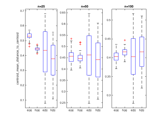
Figure 1 (left) presents the variation of the mean distance of the distances between points and the centroid feature (centroid_mean_distance_to_centroid) for hard and easy instances of the three considered sizes $25$, $50$ and $100$. Each set consists of 100 instances generated by independent runs (Mersmann et al.,, 2013). As shown in Figure 1 (left), the feature values of easy and hard instances are in different ranges. For example, for the hard instances of size $100$ the median value (indicated by the red line) is $0.4157$ while it is only $0.4032$ for the easy instances. The respective range of the feature value is $0.0577$ for the hard instances and $0.0645$ for the easy instances. For the instances generated by diversity optimization (easy and hard instances are indicated by e (b) and h (b) respectively), there is a difference in the median feature values for the hard and easy instances similar to the instances generated by the conventional approach. Additionally, the range of the feature values for both the hard and easy instances has significantly increased. For example, for the instance size $100$, the median value for easy instances is $0.4028$ and the range is $0.2382$. For the hard instances of the same size, the median is $0.04157$ while the range is $0.1917$ (see Figure 1 (left)).

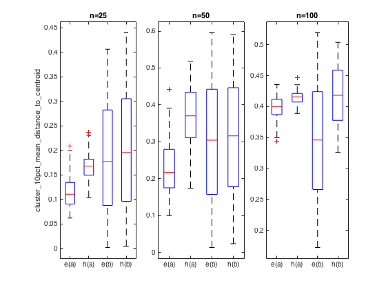
Similarly, Figure 1 (right) presents the variation of cluster $10\%$ distance to centroid (cluster_10pct_distance_to_centroid) feature for the hard and easy instances generated by the conventional approach (indicated by (e (a) and h (a)) and for the hard and easy instances generated by diversity optimization (indicated by (e (b) and h (b))). The general observations from these box plots are quite similar to the observations from the mst_dist_mean shown in Figure 1 (left). For the easy instances of size $100$, the range of the feature value is $0.0919$ for conventional instances and $0.3471$ for the instances generated by diversity optimization. Similarly, for the hard instances the range of the feature values has increased from $0.0577$ to $0.1776$ by the diversity optimization approach. As shown in Figure 1 (right), there is a significant increase in the range for other instance sizes as well. Improved ranges in feature values are observed for all considered feature.

			centroid_mean_distance_to_centroid				distance_mean				nnd_mean
n		algorithm	min	max	avg	stdev	min	max	avg	std	min	max	avg	std
25	easy	conventional	0.4603	0.5708	0.5303	0.0214	0.6125	0.7613	0.7078	0.0276	0.1923	0.4053	0.2881	0.0497
		FB-div	0.0788	0.6812	0.4570	0.0810	0.1204	0.8570	0.6139	0.1025	0.0471	0.7736	0.2884	0.0934
	hard	conventional	0.4117	0.4669	0.4446	0.0116	0.5697	0.6512	0.6126	0.0156	0.2387	0.4186	0.3161	0.0336
		FB-div	0.1076	0.5571	0.4090	0.0589	0.1641	0.7456	0.5598	0.0768	0.1033	0.7381	0.3359	0.0932
50	easy	conventional	0.4176	0.5349	0.4624	0.0287	0.5756	0.7061	0.6311	0.0310	0.1834	0.3990	0.3036	0.0479
		FB-div	0.2480	0.6456	0.4486	0.0625	0.3565	0.8200	0.6086	0.0720	0.1121	0.5538	0.3037	0.0749
	hard	conventional	0.4115	0.5185	0.4497	0.0197	0.5638	0.6752	0.6067	0.0202	0.2450	0.3852	0.3039	0.0329
		FB-div	0.2662	0.6039	0.4401	0.0506	0.3802	0.7756	0.5905	0.0611	0.1504	0.6089	0.3174	0.0551
100	easy	conventional	0.3736	0.4355	0.4047	0.0137	0.5225	0.5837	0.5540	0.0150	0.2686	0.3905	0.3241	0.0270
		FB-div	0.2789	0.5171	0.4028	0.0312	0.4027	0.6834	0.5485	0.0377	0.1909	0.4662	0.3301	0.0468
	hard	conventional	0.3954	0.4468	0.4153	0.0096	0.5408	0.6027	0.5658	0.0114	0.2971	0.3539	0.3241	0.0162
		FB-div	0.3193	0.5110	0.4146	0.0282	0.4436	0.6781	0.5628	0.0348	0.2336	0.4193	0.3254	0.0263

Table 1: In this table, for each instance size, different hardness and algorithms, the minimum value, maximum value, average value and the standard deviation are included for three different feature values, which are the centroid_mean_distance_to_centroid, distance_mean and nnd_mean. The algorithms to be compared with are the conventional approach and the feature-based diversity maximization approach.

Figure 2: $2$D Plots of feature combinations from the conventional approach. The blue dots and orange dots represent hard and easy instances respectively. The separation is mainly because the coverage of feature space is not large enough.

Figure 3: $2$D Plots of feature combinations which provide a separation between easy and hard instances. The blue dots and orange dots represent hard and easy instances respectively.

Figure 4: $2$D plots of feature combinations which do not provide a clear separation between easy and hard instances. The blue dots and orange dots represent hard and easy instances respectively.

In Table 1, some statistics are included to show the different ranges of the feature values of the instances found by the conventional approach and the diversity maximization EA. Since the conventional approach uses elitism to keep the best solution in each run, the data are gathered from $50$ independent runs of the conventional approach that generates TSP instance of acceptable quality for a certain problem size. The hard and easy instances here are classified with the same approximation ratio bound discussed previously in this section. The data to be compared with for the feature-based diversity optimization approach are obtained by a single run with population size $50$. In the table, three different features are selected from different categories to show the difference in range. From the table, it is clear that the diversity optimization approach generates TSP instances with feature values in a wider range compared to the conventional approach.

The above results suggest that the diversity optimization approach has resulted in a significant increase in the coverage over the feature space. Having the threshold for approximation ratios ($\alpha_{e}$ and $\alpha_{h}$) our method guarantees the hardness of the instances. These approximation thresholds are more extreme than the mean approximation values obtained by the conventional method. Furthermore, starting with initial population of duplicated instances and a hard coded threshold, the modified $(\mu+\lambda)$-EA is able to achieve hard instances with approximation ratio $1.347$, $1.493$ and $1.259$, respectively for instance size $25$, $50$ and $100$. The majority of the instances are clustered in a small region in the feature space while some other points are dispersed across the whole space. This is evident in the median values similar to the values for the instances with respect to conventional approach and with significantly larger range in feature value. The conventional approach has failed to explore certain regions in the feature space and missed some instances existing in those regions. Being able to discover all these instances spread in the whole feature space, our approach provides a strong basis for more effective feature based prediction.

As a result of the increased ranges and the similar gap in median feature values for hard and easy instances compared to the conventional instances, there is a strong overlap in the ranges of the features for easy and hard instances generated by the diversity optimization. This is observed in the results for mst_dist_mean and cluster_10pct_distance_to_centroid shown in Figure 1. Similar pattern holds for the other features as well. This prevents a good classification of problem instances based on single feature value.

5 Classification Based on Multiple Features

As a single feature is not capable in clearly classifying the hard/easy instances, combinations of two or three different features are examined in the following. Our analysis mainly focuses on combinations of the $7$ previously introduced features.

5.1 Diversity Maximization over Single Feature Value

Firstly, we represent the instances according to the combination of two different features in the $2$-dimensional feature value space (see Figure 3 for an example).

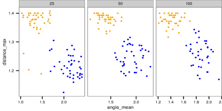
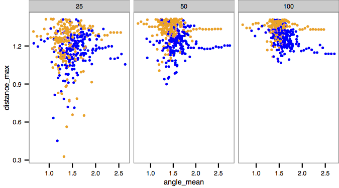
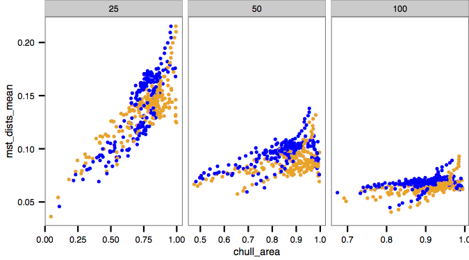
According to the observation and discussion in  (Mersmann et al.,, 2013), the two features distance _max and angle_mean can be considered together to provide an accurate classification of the hard and easy instances (see Figure 2). Whereas after increasing the diversity over the seven different feature values and a wider coverage of the $2$D space is achieved, the separation of easy and hard instances is not so obvious. Comparing to Figure 3 and  4, the clear separation shown in Figure 2 is mainly due to the instances generated from the conventional approach do not have a good coverage over the feature space. The clusters of dots representing hard and easy instances have some overlapping as shown in the left graphs of Figure 3. There are large overlapping areas lying between the two groups of instances. Another example of some separation given by two-feature combination is mst_dists_mean and chull_area which measure the mean distance of the minimum spanning tree and the area of the convex hull. However, as the number of cities in an instance increases, the overlapping area becomes larger. It is hard to do classification based on this.

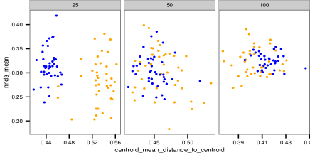
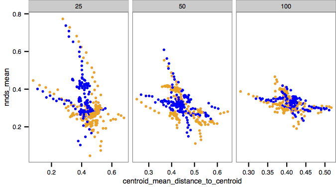
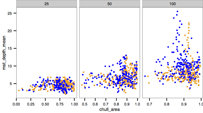
After examining the $21$ different combinations of two features out of the seven features, we found out that some combinations of two features provide a fair separation between hard and easy instances after increasing the diversity over different feature values. As shown in Figure 3, taking both mst_dists_mean and chull_area features into consideration, some separations can be spotted between hard and easy instances. However, most combinations are not able to give a clear classification between hard and easy instances, for example in Figure 4, neither the combination of features nnds_mean and centroid_mean_distance_to_centroid nor features mst_depth_mean and chull_area shows clear classification between instances of different hardness. Moreover, along with the instance size increment, the overlapping area of the dots standing for hard and easy instances grows.

Since the majority of two-feature combinations are not capable of classifying easy and hard instances, the idea of combining three different features is put forward. As in the analysis of two-feature combination, the values of the three selected features are plotted in $3$D space.

Figure 5: $3$D Plots of combining experiment results from maximizing the diversity over features mst_dists_mean, nnds_mean and chull_area, which provides a good separation of easy and hard instances. Hard and easy instances are represented as blue dots and red circles respectively. The SVM accuracy of SVM with RBF kernel is $0.9714$, $0.9857$ and $0.9667$.

Figure 6: $3$D Plots of combining experiment results from maximizing the diversity over features mst_dists_mean, chull_area and centroid_mean_distance_to_centroid, which provides a good separation of easy and hard instances. Legend is the same as that in Figure 5. The SVM accuracy of SVM with RBF kernel is $0.9714$, $0.9714$ and $0.8381$.

Figure 7: $3$D Plots of combining experiment results from maximizing the diversity over features mst_dists_mean, chull_area and mst_depth_mean, which provides a good separation of easy and hard instances. Legend is the same as that in Figure 5. The SVM accuracy of SVM with RBF kernel is $0.9476$, $0.9738$ and $0.9833$.

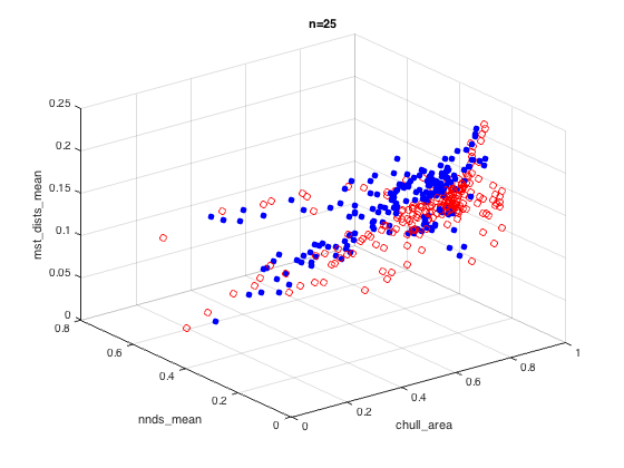
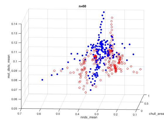
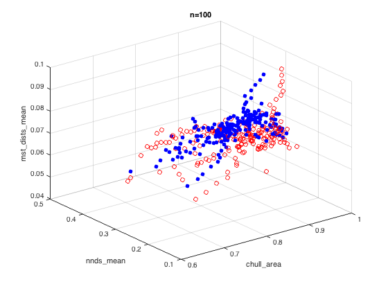
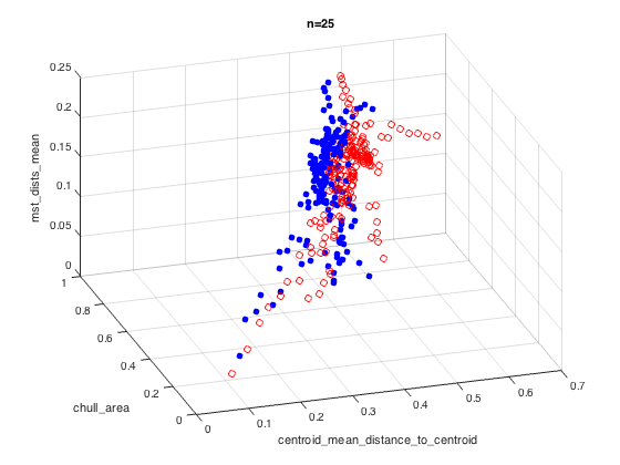
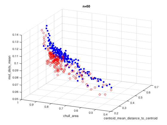
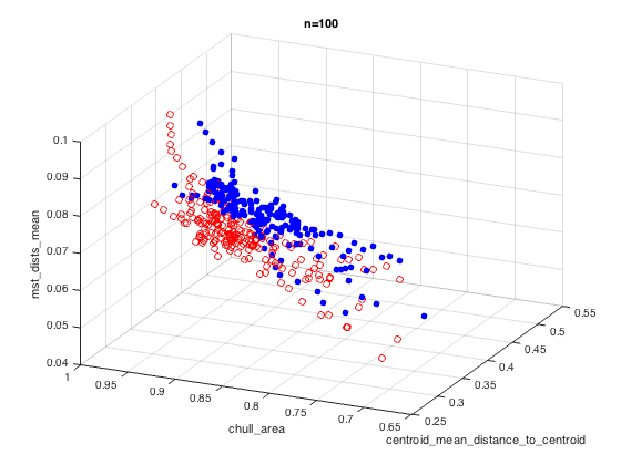
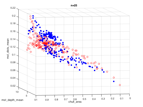
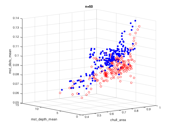
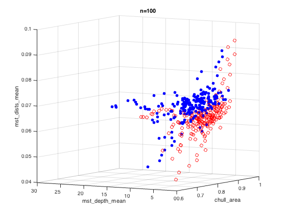
By considering a third feature in the combination, in the $35$ different combinations, it is clear that there are some separations between the two groups of $210$ instances from the $3$D-plots. A good selection of features results in an accurate classification of the instances. The three-feature combinations with the features measuring statistics about minimum spanning tree always provide good separation between hard and easy instances as shown in Figure 5 and Figure 6. Although there is an overlapping in the area between the two clusters of hard and easy instances, from the $3$D-plots, we can spot some areas where there are only dots for instances of certain hardness.

Taken another feature value into consideration, the two-feature combination that is not able to provide good separation can give some clear classification in hard and easy instances. An example illustrating this is included as Figure 7, where together with an additional feature mst_dists_mean, the two-feature combination of features mst_depth_mean and chull_area shows a clear separation between easy and hard instances comparing to the results shown in the left graph in Figure 4.

From the investigation of both the two-feature combination and three-feature combination, we found out that the range of feature values for larger TSP instances is smaller. Some of the good combinations for classifying the hardness of smaller instances may not work for larger instances, such as centroid features which perform well when combining with another feature in classifying the hardness of instances of $25$ cities while do not show a clear separation with instance size $50$ and $100$ in our study. However, there exist some three-feature combinations that give good classification of easy and hard instances without regarding to the instance size, for example mst_dists_mean, chull_area and nnds_mean, and mst_dists_mean, chull_area and mst_depth_mean.

5.2 Diversity Maximization over Multiple Feature Values

In order to examine the relationship between feature combination and hardness of the instances, a weighted population diversity based on multiple features is introduced. The weighted population diversity for a certain set of features $\{f_{1},f_{2},...,f_{k}\}$ is defined as the weighted sum of the normalised population diversity over these $k$ features. The contribution of an instance $I$ to the weighted population diversity is defined as

$$d^{\prime}(I,P)=\sum^{k}_{i=1}(w_{i}\cdot d_{f_{i}}(I,P)),$$

where $d_{f_{i}}(I,P)$ denotes the normalised contribution to the population diversity $d(I,P)$ over certain feature $i$ and $w_{i}$ represents the weight of feature $i$. The contribution of an individual to the population diversity on certain feature is normalised based on the maximum population diversity on the feature, in order to reduce the bias among different features.

This weighted population diversity is used in Algorithm 1 to gain some insight of the relationship between features combination and instance quality. The same parent and offspring population sizes are used for these experiments, which are $\mu=30$ and $\lambda=5$. The instance sizes examined are still $25$, $50$ and $100$. The $2$-OPT algorithm is executed five times to obtain the approximation quality. In the experiments, ($\mu$+$\lambda$)-EA_D execute for $10,000$ generation as previous. Since it is shown in Section 4 that a combination of three features is able to provide a good separation between hard and easy instances, some of the good three-feature combinations are chosen for exploration. The weight distributions for $\{f_{1},f_{2},f_{3}\}$ considered in the experiments are $\{1,1,1\}$, $\{2,1,1\}$, $\{1,2,1\}$, $\{1,1,2\}$, $\{2,2,1\}$, $\{2,1,2\}$, $\{1,2,2\}$. The same hardness thresholds are used in these experiments as previous. After the seven independent runs for easy and hard instances, the final solution sets are put together. Therefore the results set has $210$ instances for each instance size and hardness type, which is the same as previous experiments. The results are plotted in $3$D space and compared to the previous experiments on single feature discussed in Section 3 and  4.

The weighted population diversity offers a way to examine the overlapping area of hard and easy instances. With the weighting technique, it takes consideration about the relationship between the different features examined. Since most of these features are not independent from each others and the weighted population diversity considers multiple features at the same time, it is predictable that with the weighted population diversity the extreme value for each single feature may not reach.

Figure 8: $3$D Plots of combining experiment results from maximizing the diversity over features mst_dists_mean, nnds_mean and chull_area with considering of weighting, which provides a good separation of easy and hard instances. Hard and easy instances are represented as blue dots and orange dots respectively.

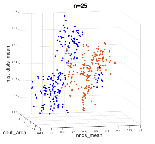
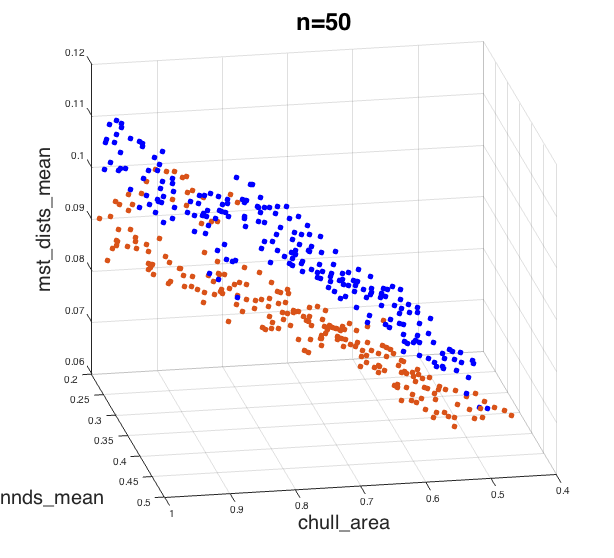
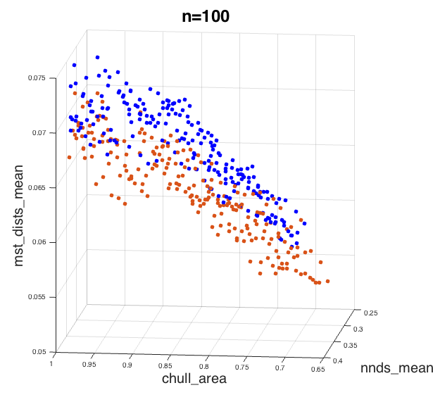
An example is shown in Figure 8 focusing on maximizing the weighted population diversity over the combination of features mst_dists_mean, nnds_mean and chull_area, which is shown to be a good combination for separating the hard and easy instances. From the comparison between Figure 5 and Figure 8, we can see that although the results from maximizing weighted population diversity does not cover a wider search space, it provides a detailed insight into the intersection between the hard and easy instances. The $3$D plots of different instance sizes show that the combination of these three certain features provide a clear separation between hard and easy instances. There are some overlapping areas in the search space, but it is clear that this combination of features provide some hints for predicting of hard or easy instances. It is expected that additional features might increase the separability. Because each additional feature contributes to an additional constraint on the hard/easy classification. However, due to visualization limitations we consider up to 3 features for graphical analysis.

6 Instances Classification Using Support Vector Machine

Support vector machines (SVMs) are well-known supervised learning models in machine learning which can be used for classification, regression and outliers detection  (Cortes and Vapnik,, 1995; Gunn,, 1998). In order to quantify the separation between instances of different hardness based on the feature values, SVM models are constructed for each combination of features.

6.1 Linear SVM

The linear classifier is the first model tried in classifying the dataset. In SVM the linear classifiers that can separate the data with maximum margin is termed as the optimal separating hyper-plane. From the plots in Figure 3, 4, 5 and 6, it is clear that none of the datasets are linearly separable. Taken the trade-off between maximizing the margin and minimizing the number of misclassified data points into consideration, the soft-margin SVM is used for classification.

Let $ACC_{n}$ be the training accuracy of a feature combination in separating the hard and easy instances of size $n$. We define $ACC_{n}$ as the ratio of number of instances which are correctly classified by the model to the total number of instances in the dataset. All classification experiments are done in R with library$\{e1071\}$ (Meyer et al.,, 2015). The training data of the SVM models are the population of 420 instances generated as in Section 3 and the training accuracy is regarded as a quantified measurement of the separation between hard and easy instances. The feature combinations used for classification are the $21$ two-feature combinations and $35$ three-feature combinations discussed in Section 5.

From experiment results, $ACC_{25}$ for two-feature combinations lie in the range of $0.5095$ to $0.7548$ with an average accuracy of $0.6672$, while the $ACC_{25}$ for three-feature combinations lie between $0.6286$ to $0.7786$ with average value $0.7079$. In the case of instances with city number of $50$, two-feature combination results in $ACC_{50}$ lying in the range of $0.5286$ to $0.7738$ with an average of $0.6544$ while $ACC_{50}$ of three-feature combinations are from $0.5381$ to $0.85$ with average accuracy equal to $0.6969$. For larger instance size, $ACC_{100}$ are in the range between $0.5738$ and $0.8119$ with average $0.6986$ for two-feature combinations, whereas those for three-feature combinations lie in the scope of $0.6238$ to $0.8524$ with average $0.7382$.

Although three-feature combinations show better accuracy in separation of hard and easy instances than those two-feature combinations, there is no significant difference in $ACC$ for two-feature combinations and three-feature combinations. Moreover, the general low accuracy implies the high possibility that the linear models are not suitable for separating the hard and easy instances based on most of the feature combinations.

We then move to applying kernel function for non-linear mapping of the feature combination.

6.2 Nonlinear Classification with RBF Kernel

The linearly non-separable features can become linearly separable after mapped to a higher dimension feature space. The Radial Basis Function (RBF) kernel is one of the well-known kernel function used in SVM classification.

There are two parameters need to be selected when applying RBF, which are $C$(cost) and $\gamma$. The parameter setting for RBF is crucial, since increasing $C$ and $\gamma$ leads to accurate separation of the training data but at the same time causes over-fitting Cherkassky and Ma, (2004). The SVMs here are generated for quantifying the separation rate between hard and easy instances rather than constructing a model for classification of other instances. After some initial trials, $(C,\gamma)$ is set to $(100,2)$ in all the tests to avoid over-fitting to the selected training set. This parameter setting may not be the best parameters for the certain feature combination in SVM classifying, but it helps us to gain some understanding of the separation of hard and easy instances generated from previous experiments based on the same condition.

Table 2 and  3 show the accuracy of different two features or three features combination in hard and easy instances separation. With RBF kernel, SVM with certain parameter setting can generate a model separating the dataset with average accuracy of $0.8170$, $0.8244$ and $0.8346$ in $2$D feature space for instance size $25$, $50$ and $100$ respectively. Whereas with three features, SVM with the same parameter setting provides a separation with average accuracy of $0.9503$, $0.9584$ and $0.9422$ for instance size $25$, $50$ and $100$ respectively.

From the results, it can be concluded that there are better separations between hard and easy instances in the $3$D feature space.

Feature 1	Feature 2	$ACC_{25}$	$ACC_{50}$	$ACC_{100}$
angle_mean	centroid_mean_distance_to_centroid	0.8476	0.8071	0.8071
angle_mean	chull_area	0.7857	0.7810	0.7929
angle_mean	cluster_10pct_mean_distance_to_centroid	0.7810	0.7786	0.8000
angle_mean	mst_depth_mean	0.7524	0.7381	0.8000
angle_mean	nnds_mean	0.8167	0.8833	0.8452
angle_mean	mst_dists_mean	0.8119	0.8024	0.8405
centroid_mean_distance_to_centroid	chull_area	0.8619	0.7667	0.8381
centroid_mean_distance_to_centroid	cluster_10pct_mean_distance_to_centroid	0.8524	0.8357	0.7548
centroid_mean_distance_to_centroid	mst_depth_mean	0.8381	0.7643	0.8095
centroid_mean_distance_to_centroid	nnds_mean	0.8786	0.9524	0.8476
centroid_mean_distance_to_centroid	mst_dists_mean	0.8905	0.8571	0.8762
chull_area	cluster_10pct_mean_distance_to_centroid	0.8000	0.7881	0.8548
chull_area	mst_depth_mean	0.7429	0.7429	0.7571
chull_area	nnds_mean	0.8071	0.8905	0.8452
chull_area	mst_dists_mean	0.8619	0.8643	0.9024
cluster_10pct_mean_distance_to_centroid	mst_depth_mean	0.7619	0.7714	0.7929
cluster_10pct_mean_distance_to_centroid	nnds_mean	0.8190	0.8833	0.8643
cluster_10pct_mean_distance_to_centroid	mst_dists_mean	0.8095	0.8095	0.8738
mst_depth_mean	nnds_mean	0.7786	0.8595	0.8405
mst_depth_mean	mst_dists_mean	0.8095	0.8214	0.8810
nnds_mean	mst_dists_mean	0.8500	0.9143	0.9024

Table 2: This table lists the accuracy of SVM with RBF kernel separating the hard and easy instances in 21 different two-feature space.

Feature 1	Feature 2	Feature 3	$ACC_{25}$	$ACC_{50}$	$ACC_{100}$
angle_mean	centroid_mean_distance_to_centroid	chull_area	0.9500	0.9190	0.9452
angle_mean	centroid_mean_distance_to_centroid	cluster	0.9405	0.9357	0.8214
angle_mean	centroid_mean_distance_to_centroid	mst_depth_mean	0.9548	0.9548	0.9214
angle_mean	centroid_mean_distance_to_centroid	nnds_mean	0.9452	0.9952	0.9833
angle_mean	centroid_mean_distance_to_centroid	mst_dists_mean	0.9571	0.9500	0.9524
angle_mean	chull_area	cluster	0.9524	0.9310	0.8881
angle_mean	chull_area	mst_depth_mean	0.9357	0.9238	0.9500
angle_mean	chull_area	nnds_mean	0.9405	0.9714	0.9571
angle_mean	chull_area	mst_dists_mean	0.9667	0.9619	0.9143
angle_mean	cluster	mst_depth_mean	0.9214	0.9143	0.9810
angle_mean	cluster	nnds_mean	0.9476	0.9690	0.9333
angle_mean	cluster	mst_dists_mean	0.9571	0.9143	0.9405
angle_mean	mst_depth_mean	nnds_mean	0.9310	0.9762	0.9238
angle_mean	mst_depth_mean	mst_dists_mean	0.9476	0.9262	0.9476
angle_mean	nnds_mean	mst_dists_mean	0.9429	0.9762	0.8833
centroid_mean_distance_to_centroid	chull_area	cluster	0.9476	0.9333	0.9310
centroid_mean_distance_to_centroid	chull_area	mst_depth_mean	0.9595	0.8762	0.9762
centroid_mean_distance_to_centroid	chull_area	nnds_mean	0.9667	0.9881	0.9929
centroid_mean_distance_to_centroid	chull_area	mst_dists_mean	0.9714	0.9714	0.8381
centroid_mean_distance_to_centroid	cluster	mst_depth_mean	0.9476	0.9286	0.8571
centroid_mean_distance_to_centroid	cluster	nnds_mean	0.9643	0.9905	0.8810
centroid_mean_distance_to_centroid	cluster	mst_dists_mean	0.9500	0.9595	0.9190
centroid_mean_distance_to_centroid	mst_depth_mean	nnds_mean	0.9500	0.9881	0.9595
centroid_mean_distance_to_centroid	mst_depth_mean	mst_dists_mean	0.9548	0.9548	0.9595
centroid_mean_distance_to_centroid	nnds_mean	mst_dists_mean	0.9667	1.0000	0.9952
chull_area	cluster	mst_depth_mean	0.9286	0.9524	0.9333
chull_area	cluster	nnds_mean	0.9524	0.9667	0.9667
chull_area	cluster	mst_dists_mean	0.9595	0.9595	0.9929
chull_area	mst_depth_mean	nnds_mean	0.9381	0.9857	0.9476
chull_area	mst_depth_mean	mst_dists_mean	0.9476	0.9738	0.9833
chull_area	nnds_mean	mst_dists_mean	0.9714	0.9857	0.9667
cluster	mst_depth_mean	nnds_mean	0.9214	0.9857	0.9738
cluster	mst_depth_mean	mst_dists_mean	0.9500	0.9476	0.9643
cluster	nnds_mean	mst_dists_mean	0.9643	0.9833	0.9976
mst_depth_mean	nnds_mean	mst_dists_mean	0.9429	0.9929	0.9929

Table 3: This table lists the accuracy of SVM with RBF kernel separating the hard and easy instances in 35 different three-feature space. The cluster feature in the table refers to the cluster_10pct_mean_distance_to_centroid feature.

7 Diversity optimization for Instance Hardness

In the experiments in previous sections, the main focus of diversity maximization is the feature values. The quality of solutions is guaranteed by a predefined threshold. In order to have an insight into the relationship between the feature values and problem hardness, we conduct another experiment about population diversity optimization with instance hardness. The experiment is based on the TSP and Algorithm 1 as well. In this case, the approximation ratio is taken as a feature value. Maximizing the diversity over approximation ratio results in a set of individuals with different quality. By doing this, we obtain knowledge about the relationship between feature values and instance hardness from another point of view.

1 Initialize the population $P$ with $\mu$ TSP instances of certain size.

2 Let $C\subseteq P$ where $|C|=\lambda$.

3 For each $I\in C$, produce an offspring $I^{\prime}$ of $I$ by mutation and add $I^{\prime}$ to $P$.

4 While $|P|>\mu$, remove an individual $I=\arg\min_{J\in P}d_{ar}(J,P)$ uniformly at random.

5 Repeat step 2 to 4 until termination criterion is reached.

Algorithm 2 $(\mu+\lambda)$-$EA_{DA}$

In this case, the algorithm needs to be modified in the solution quality check phase. The evolutionary algorithm without hard coded solution quality threshold is shown in Algorithm 2. The population diversity measurement $d_{ar}(I,P)$ in step 4 follows the formulation proposed in Section 3 with the approximation ratio as the target feature value. In the survivor selection phase, the individual that contributes the least to the population diversity over approximation ratio is removed.

For the purpose of reasonable coverage over the whole space, the population size and offspring population size is set to $400$ and $10$ respectively, in this experiment. The other parameters are all kept the same with previous experiments. Then the R program is run for 30,000 generations to obtain some stable results.

Figure 9: $3$D Plots of experiment results from maximizing the diversity over approximation ratio in the feature space of feature combination chull_area, mst_dist_mean and mst_depth_mean. The color of the dot reflects the hardness of the problem and the easier problem is indicated with lighter color.

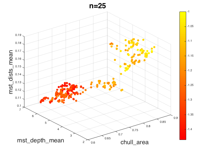
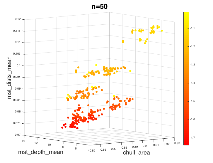
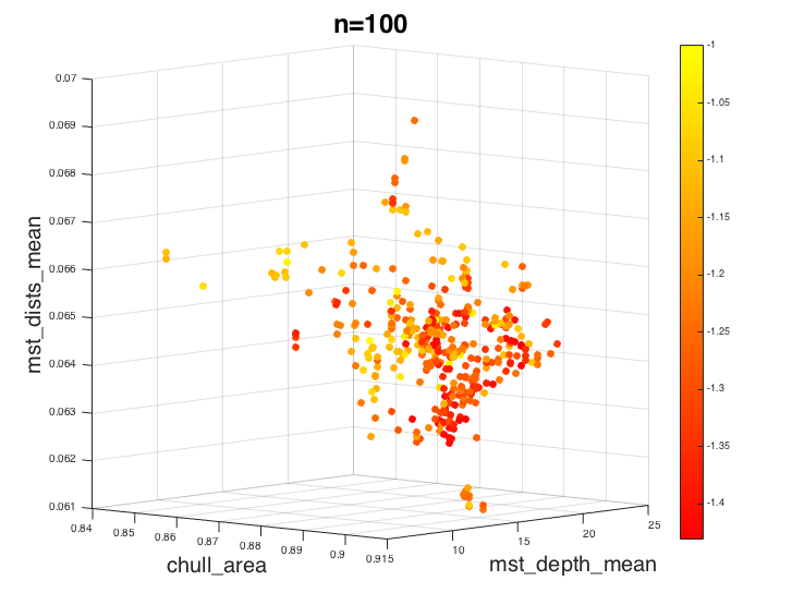
Figure 9 and 10 show some example $3$D plots of the experimental results. The $400$ individuals are plotted in the $3$D feature space with consideration over different feature combinations. The vertical colorbar lying on the right side of each plot illustrates the relationship between color and problem hardness and indicates the mapping of approximation ratio into the different colors. The dots in lighter color imply easier instances.

The plots in Figure 9 present the resulting instances in the space of feature chull_area, mst_dist_mean and mst_depth_mean. There is clear separation between the red dots and yellow dots in the figure for different problem sizes. The red and yellow dots refer to instances with extreme approximation ratio in each case. For larger instances, there is no clear cluster of instances with different hardness but we can still find areas where hard or easy instances gather. On the other hand, for problem instances with approximation ratio lying in the range of $1.1$ to $1.2$, $1.2$ to $1.4$ and $1.15$ to $1.2$ which are represented by orange dots in the plots, the locations are hard to classify.

Figure 10: $3$D Plots of experiment results from maximizing the diversity over approximation ratio in the feature space of feature combination chull_area, angle_mean and cluster_$10$pct_mean_distance_to_centroid. The colors of the dots reflect the hardness of the problem.

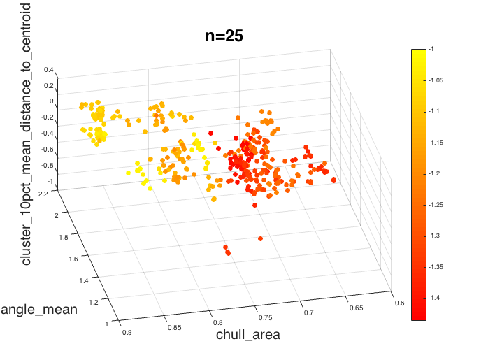
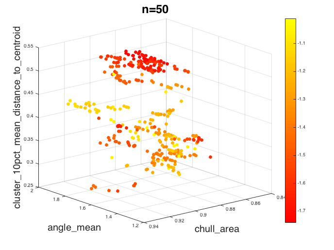
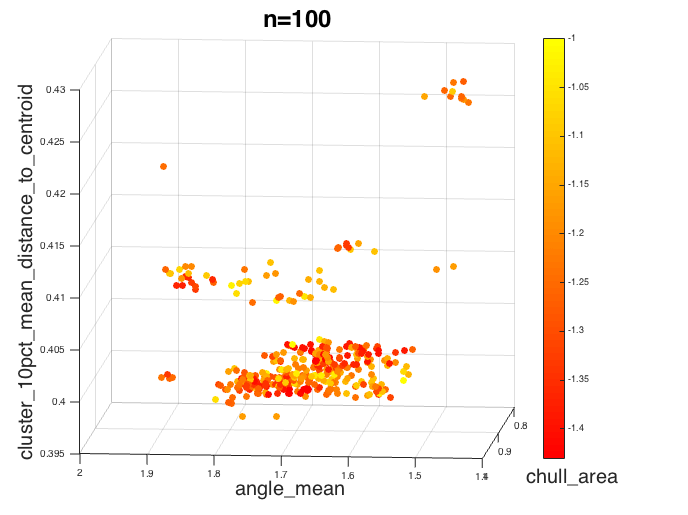
The plots in Figure 10 show the relationship of problem hardness with the feature combination chull_area, angle_mean and cluster_$10$pct_mean_distance_to_centroid. Similar observation can be obtained. The separation for problem size $25$ is clear. However, when the number of cities in each instance increases, the overlapping area becomes larger.

Algorithm 2 allows us to generate a set of solutions with different hardness. The approximation ratio for problem size $25$, $50$ and $100$ is maximized to $1.434$, $1.739$ and $1.430$ in this experiment which implies the populations cover a even wider range than those from previous experiments.

8 Conclusions

With this paper, we have introduced a new methodology of evolving easy/hard instances which are diverse with respect to feature sets of the optimization problem at hand. Using our diversity optimization approach we have shown that the easy and hard instances obtained by our approach cover a much wider range in the feature space than previous methods. The diversity optimization approach provides instances which are diverse with respect to the investigated features. The proposed population diversity measurements provide a good evaluation of the diversity over single or multiple feature values. Our experimental investigations for $2$-OPT and TSP provide evidence that the large set of diverse instances can be classified quite well into easy and hard instances when considering a suitable combination of multiple features which provide some guidance for predication as the next step. In particular, the SVM classification model built with the diverse instances that can classify TSP instances based on problem hardness provides a strong basis for future performance prediction models that lead to automatic algorithm selection and configuration. Building such models would require further experimentation to determine the minimal set of strong features that can predict performance accurately.

References

- Alexander et al., (2017) Alexander, B., Kortman, J., and Neumann, A. (2017). Evolution of artistic image variants through feature based diversity optimisation. In Proceedings of the Genetic and Evolutionary Computation Conference, GECCO 2017, Berlin, Germany, July 15-19, 2017, pages 171–178.
- Applegate et al., (2002) Applegate, D., Cook, W., Dash, S., and Rohe, A. (2002). Solution of a min-max vehicle routing problem. INFORMS Journal on Computing, 14(2):132–143.
- Cherkassky and Ma, (2004) Cherkassky, V. and Ma, Y. (2004). Practical selection of svm parameters and noise estimation for svm regression. Neural Networks, 17(1):113 – 126.
- Cortes and Vapnik, (1995) Cortes, C. and Vapnik, V. (1995). Support-vector networks. Machine Learning, 20(3):273–297.
- Croes, (1958) Croes, G. A. (1958). A method for solving traveling-salesman problems. Operations Research, 6(6):791–812.
- Eggensperger et al., (2015) Eggensperger, K., Hutter, F., Hoos, H. H., and Leyton-Brown, K. (2015). Efficient benchmarking of hyperparameter optimizers via surrogates. In Proceedings of the Twenty-Ninth AAAI Conference on Artificial Intelligence, January 25-30, 2015, Austin, Texas, USA., pages 1114–1120.
- Englert et al., (2014) Englert, M., Röglin, H., and Vöcking, B. (2014). Worst case and probabilistic analysis of the 2-opt algorithm for the TSP. Algorithmica, 68(1):190–264.
- Feurer et al., (2015) Feurer, M., Springenberg, J. T., and Hutter, F. (2015). Initializing bayesian hyperparameter optimization via meta-learning. In Proceedings of the Twenty-Ninth AAAI Conference on Artificial Intelligence, January 25-30, 2015, Austin, Texas, USA., pages 1128–1135.
- Gao et al., (2016) Gao, W., Nallaperuma, S., and Neumann, F. (2016). Feature-based diversity optimization for problem instance classification. In Parallel Problem Solving from Nature - PPSN VII, 7th International Conference, Edingburgh, UK, September 17-21, 2016, Proceedings.
- Gunn, (1998) Gunn, S. R. (1998). Support vector machines for classification and regression.
- Hutter et al., (2014) Hutter, F., Xu, L., Hoos, H. H., and Leyton-Brown, K. (2014). Algorithm runtime prediction: Methods & evaluation. Artif. Intell., 206:79–111.
- Kötzing et al., (2012) Kötzing, T., Neumann, F., Röglin, H., and Witt, C. (2012). Theoretical analysis of two ACO approaches for the traveling salesman problem. Swarm Intelligence, 6(1):1–21.
- Mersmann et al., (2013) Mersmann, O., Bischl, B., Trautmann, H., Wagner, M., Bossek, J., and Neumann, F. (2013). A novel feature-based approach to characterize algorithm performance for the traveling salesperson problem. Annals of Mathematics and Artificial Intelligence, 69(2):151–182.
- Meyer et al., (2015) Meyer, D., Dimitriadou, E., Hornik, K., Weingessel, A., and Leisch, F. (2015). e1071: Misc Functions of the Department of Statistics, Probability Theory Group (Formerly: E1071), TU Wien. R package version 1.6-7.
- Nallaperuma et al., (2014) Nallaperuma, S., Wagner, M., and Neumann, F. (2014). Parameter prediction based on features of evolved instances for ant colony optimization and the traveling salesperson problem. In PPSN XIII - 13th International Conference, Ljubljana, Slovenia, September 13-17, 2014. Proceedings, pages 100–109.
- Nallaperuma et al., (2013) Nallaperuma, S., Wagner, M., Neumann, F., Bischl, B., Mersmann, O., and Trautmann, H. (2013). A feature-based comparison of local search and the christofides algorithm for the travelling salesperson problem. In FOGA ’13, pages 147–160.
- Neumann et al., (2018) Neumann, A., Gao, W., Doerr, C., Neumann, F., and Wagner, M. (2018). Discrepancy-based evolutionary diversity optimization. In Proceedings of the Genetic and Evolutionary Computation Conference, GECCO 2018, Kyoto, Japan, July 15-19, 2018, pages 991–998.
- Neumann et al., (2019) Neumann, A., Gao, W., Wagner, M., and Neumann, F. (2019). Evolutionary diversity optimization using multi-objective indicators. In Auger, A. and Stützle, T., editors, Proceedings of the Genetic and Evolutionary Computation Conference, GECCO 2019, Prague, Czech Republic, July 13-17, 2019, pages 837–845. ACM.
- Neumann and Witt, (2010) Neumann, F. and Witt, C. (2010). Bioinspired Computation in Combinatorial Optimization:Algorithms and Their Computational Complexity. Springer-Verlag New York, Inc., New York, NY, USA, 1st edition.
- R Core Team, (2015) R Core Team (2015). R: A Language and Environment for Statistical Computing. R Foundation for Statistical Computing, Vienna, Austria.
- Smith-Miles and Bowly, (2015) Smith-Miles, K. and Bowly, S. (2015). Generating new test instances by evolving in instance space. Computers & OR, 63:102–113.
- Smith-Miles and Lopes, (2012) Smith-Miles, K. and Lopes, L. (2012). Measuring instance difficulty for combinatorial optimization problems. Computers & OR, 39(5):875–889.
- Smith-Miles et al., (2010) Smith-Miles, K., van Hemert, J., and Lim, X. Y. (2010). Understanding TSP difficulty by learning from evolved instances. In 4th International Conference on Learning and Intelligent Optimization (LION), LION’10, pages 266–280. Springer.
- (24) Ulrich, T., Bader, J., and Thiele, L. (2010a). Defining and optimizing indicator-based diversity measures in multiobjective search. In Parallel Problem Solving from Nature - PPSN XI, 11th International Conference, Kraków, Poland, September 11-15, 2010, Proceedings, Part I, pages 707–717.
- (25) Ulrich, T., Bader, J., and Zitzler, E. (2010b). Integrating decision space diversity into hypervolume-based multiobjective search. In Genetic and Evolutionary Computation Conference, GECCO 2010, Proceedings, Portland, Oregon, USA, July 7-11, 2010, pages 455–462.
- van Hemert, (2006) van Hemert, J. I. (2006). Evolving combinatorial problem instances that are difficult to solve. Evolutionary Computation, 14(4):433–462.
- Vilalta and Drissi, (2002) Vilalta, R. and Drissi, Y. (2002). A perspective view and survey of meta-learning. Artificial Intelligence Review, 18(2):77–95.
- Xu et al., (2008) Xu, L., Hutter, F., Hoos, H. H., and Leyton-Brown, K. (2008). Satzilla: portfolio-based algorithm selection for sat. Journal of Artificial Intelligence Research, 32(1):565–606.