Writhe induced phase transition in unknotted self-avoiding polygons.

Abstract

Recently it has been argued that weighting the writhe of unknotted self-avoiding polygons can be related to possible experiments that turn double stranded DNA. We first solve exactly a directed model and demonstrate that in such a subset of polygons the problem of weighting their writhe is associated with a phase transition. We then analyse simulations using the Wang-Landau algorithm to observe scaling in the fluctuations of the writhe that is compatible with a second-order phase transition in a undirected self-avoiding polygon model. The transition can be clearly detected when the polygon is stretched with a strong pulling force.

1 Introduction

Over the past two decades, experiments [1, 2, 3, 4, 5, 6, 7] that turn single molecules of twist-storing polymers like DNA have been performed. A DNA molecule which is pulled and twisted simultaneously can move from a stretched state into a state induced by supercoiling [1]. The conformational transition associated with these experiments attracts continuing interest.

Figure 1.1: Sketch of the thought experiment. Both sides of a DNA like polymer are attached to the apparatus. The depicted cylinder can be rotated (black arrows). The twist-storing polymer exerts a force $f$ on the cylinder which attacks at a distance $r$ from the centre (green arrow). On the other hand, a force $F$ (red arrow) can be applied at a distance $R$ from the centre. Then, the net torque exerted on the cylinder reads $F\,R-f\,r$.

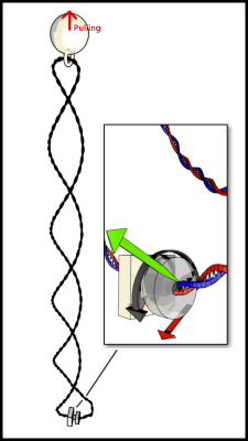
We propose a thought experiment that is slightly different from the experiments currently performed on DNA. We consider a two sided apparatus as shown in Figure 1.1. On one side the twist-storing polymer is attached to an immobile part of the apparatus, on the other side, the twist-storing polymer is connected to a turn-able cylindrical structure, which is used to control the linking number between the two strands of the double stranded molecule. In order to apply a pulling force, we take a magnetic bead, attach a loop to it and pass one end of the twist-storing polymer through the loop before it is attached to the apparatus. Via a magnetic field, a constant pulling force can be applied to the polymer. Note that the force does not attack at a specific point of the twist-storing polymer. In fact, it is important that there is as little as possible interaction between the loop material and the twist-storing. Instead of controlling the number of turns, we can imagine to keep the polymer at a constant torque $\beta_{l}$. This is called the constant torque ensemble.

In the literature [8, 9, 10, 11, 12, 13, 14] the mechanics of twist-storing double-stranded DNA has been modeled using ribbons [9, 15, 16, 17]. The boundary curves of the ribbon can be thought to represent the strands of a DNA molecule. Only if the knot type of the polymer is conserved, the linking number between these curves is controlled by the number of turns and according to the CFW theorem [9, 15, 16, 17], the linking number can be absorbed either in the form of twist or in the form of writhe,

$$Lk=Wr+Tw\,.$$ (1.1)

In this paper, we wish to use a lattice model of ribbons [18, 19]. Conveniently, the linking number of a lattice ribbon was recently proved to be equal to the writhe of the centre line of the lattice ribbon in [20], itself a self-avoiding polygon on the sc lattice. In this way, we use a single self-avoiding polygon instead of the more complicated model of lattice ribbons. While not every self-avoiding polygon on the simple cubic lattice can be the centre line of the lattice ribbon, the condition for polygons that are is merely local, so that we conjecture that the critical structure remains unaffected by extending the ensemble to all SAPs. Therefore, we model our thought experiment by weighting the writhe of self-avoiding polygons (SAP) on the simple cubic (sc) lattice. We are interested in observing the typical signs that are associated with real phase transitions.

2 Model

2.1 The SAW as model of phase transitions

The self-avoiding walk (SAW) in three dimensions is one of the simplest models of polymers [21]. It reduces polymers down to two features. First, it represents the fact that a polymer is composed from a large number of repeating subunits. Second, the self-avoidance reflects the fact that polymers cannot be compressed arbitrarily. As a model of long polymers in statistical mechanics, the SAW is known to make correct predictions about the scaling of the end-to-end distance or equivalently the radius of gyration of a polymer in a good solvent at thermal equilibrium. When we denote the length of the SAW by $n$, the expectation value of the squared radius of gyration is predicted to obey the scaling form

$$\left\langle R_{g}^{2}\right\rangle_{n}=A_{g}\,n^{2\,\nu}\left(1+b_{g}\,n^{-\Delta}+\ldots\right)$$ (2.1)

where $A_{g}$ and $b_{g}$ are constants specific to the lattice on which the SAW lives. In contrast, the exponents $\nu$ and $\Delta$ are considered to be universal. They have been determined from simulations [22] as well as from calculations in the context of the renormalization group idea. This is due to a mapping of the SAW onto the magnetic $N$-vector model in the formal limit $N\rightarrow 0$. Recent predictions [23] are $\nu=0.587597\pm 0.000007$ and $\Delta=0.528\,\pm 0.012$. The predictions for the leading scaling exponent $\nu$ agree with experiments on DNA [24] that for long molecules of DNA fit their results to $\left\langle R_{g}\right\rangle\sim L^{\nu}$, where $L$ is the length of the DNA.

In addition SAWs are used as configurations of various standard models of single polymer phase transitions. Most notable are the collapse and adsorption transitions. In the latter case, one considers all SAWs above a plane in three dimensions or above a line in two dimensions and weights the SAWs by the number of contacts made with the wall (surface or line, respectively). Denote a SAW by $\varphi=\left\{\varphi_{i}\right\}_{i=1,..,n+1}$, where $\varphi_{i}$ are the vertices. Denote by $a$ the number of visits to the wall, then the SAWs of length $n$ are distributed according the Boltzmann distribution

$$p\left(\varphi\right)=Z_{n}^{-1}\,e^{\beta_{a}a\left(\varphi\right)},$$ (2.2)

where $a\left(\varphi\right)$ measures the number of visits in $\varphi$, $Z_{n}=\sum_{\varphi\in\Omega_{n}}e^{\beta_{a}a\left(\varphi\right)}$ is the partition function and $\beta_{a}$ is related to the interaction strength between the polymer and the wall. We remark that we use the subscript in the coupling $\beta_{a}$ only as a label, not an index so that when we denote by $C_{n\,a}$ the number of SAWs of length $n$ with $a$ visits, we may write the partition function as

$$Z_{n}\left(\beta_{a}\right)=\sum_{a}C_{n\,a}e^{\beta_{a}\,a}.$$ (2.3)

The finite size free energy is defined as $f_{n}\left(\beta_{a}\right)=n^{-1}\log Z_{n}\left(\beta_{a}\right)$ so that in the thermodynamic limit $n\rightarrow\infty$, it is known that there is a critical value $\beta_{a}^{\left(\infty\right)}$ at which the free energy $f=\lim_{n\rightarrow\infty}f_{n}$ becomes non-analytic. When the critical value is crossed from below the system undergoes a continuous phase transition from a desorbed phase into the adsorbed phase. In the desorbed phase the first derivative of the free energy with respect to $\beta_{a}$ vanishes, while in the adsorbed phase a certain fraction of the vertices is expected to be in contact with the wall. Correspondingly, the transition is associated with a discontinuity in the second derivative $\partial^{2}f\left(\beta_{a}\right)/\partial\beta_{a}^{2}$, which jumps from zero to some finite value at $\beta_{a}^{\left(\infty\right)}$. At finite size, the singular part of the free energy near $\beta_{a}^{\left(\infty\right)}$ obeys a standard scaling Ansatz

$$f_{n}^{\left(sing\right)}\left(\tau\right)=n^{-1}\,h\left(n^{\phi}\tau\right).$$ (2.4)

where $\tau=\beta_{a}-\beta_{a}^{\left(\infty\right)}$, $h\left(x\right)$ is a scaling function and $\phi$ is called the crossover exponent. In the case of the adsorbed walk, the crossover exponent takes a mean field value of $1/2$ at the transition [25]. An exact solution for certain directed SAWs in two dimensions is given in [26], which also includes an expression for the scaling function. In the following, we will consider SAP which are SAWs, the first and last vertex of which are adjacent.

2.2 The Writhe of SAPs on the sc lattice

The writhe is a quantity associated with the topology and geometry of a space curve. For a $C^{1}$ curve $R$, it is given by

$$Wr\left(R\right)=\frac{1}{4\pi}\int_{S^{2}}d\mathbf{d}\,Lk\left(R,\,R+\epsilon\mathbf{d}\right),$$ (2.5)

where $Lk\left(R,\,R+\epsilon\mathbf{d}\right)$ is the linking number between the curve $R$ and a copy of $R$ pushed off into the direction of $\mathbf{d}$.

In the lattice polymer literature [27, 28, 29, 30, 31], the writhe of a SAP is usually computed based on a theorem by Laing and Sumners [32], who realized that the expression for the writhe simplifies for a SAP $\varphi$ on the sc lattice by considering the linking number between $\varphi$ and four copies of it translated by $\mathbf{d}=\left(\pm 1/2,\,\pm 1/2,\,\pm 1/2\right)$, leading to

$$Wr\left(\varphi\right)=\frac{1}{4}\,\left\{Lk\left(\varphi,\,\varphi+\frac{1}{2}\left(1,\,1,\,1\right)^{T}\right)+Lk\left(\varphi,\,\varphi+\frac{1}{2}\left(1,\,-1,\,1\right)^{T}\right)+...\right\}.$$ (2.6)

It was shown in [33] that this can further be rewritten as

$$Wr\left(\varphi\right)=Lk\left(\varphi,\,\varphi+\frac{1}{2}(1,1,1)^{T}\right)-\frac{1}{8}\sum_{i=1}^{n}\left[\hat{\varphi}_{i-1},\,\hat{\varphi}_{i},\,(1,1,1)^{T}\right]\left\langle(1,1,1)^{T},\,\hat{\varphi}_{i-1}+\hat{\varphi}_{i}\right\rangle.$$ (2.7)

where the square brackets denote the triple product and $\hat{\varphi_{i}}$ denotes the unit vector from $\varphi_{i}$ to $\varphi_{i+1}$. It is this latter formula that will be used in our simulations.

2.3 Model: Self-Avoiding Unknot on the sc lattice

Figure 2.1: A self-avoiding unknot (SAUK) above a surface of length $n=28$. The step furthest away from the surface defines the extension $h$.

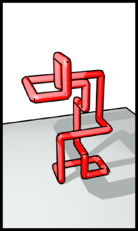
As mentioned in the introduction, we consider a model in which we weight the writhe of self-avoiding polygons on the sc lattice. To model our thought experiment, we need to restrict the knot type of the self-avoiding polygons to be the unknot. We refer to these as self-avoiding unknots (SAUK). Imagine a surface at $x_{3}=0$, so that the SAUK is tethered to the origin and restricted to the positive half space $\left(\varphi_{i}\right)_{3}\geq 0$. In the thought experiment, the energy associated with pulling is proportional to the distance $h$ of the bead from the plane $x_{3}=0$. At least for strong pulling forces this should typically be identical to the $x_{3}$-component of the vertex furthest away from the surface. We define

$$h=\max_{i=1,..,n}\left(\varphi_{i}\right)_{3}.$$ (2.8)

The second parameter $w$ is an appropriate multiple of the writhe. Then, the partition function reads

$$Z_{n}\left(\beta_{l},\,\beta_{h}\right)=\sum_{w,\,h}C_{n\,w\,h}e^{\beta_{l}w+\beta_{h}h}\,,$$ (2.9)

where $C_{n\,w\,h}$ is the number of SAUKs of length $n$, writhe $w$ and extension $h$. The finite size free energy is given by $f_{n}\left(\beta_{l},\,\beta_{h}\right)=n^{-1}\log\,Z_{n}\left(\beta_{l},\,\beta_{h}\right)$.

2.4 Overview

The remainder of this paper is structured as follows. In Section 3 we will define a directed version of a SAUK. We use it to show via an exact solution that weighting the writhe of certain unknotted polygons induces a real phase transition. By construction, this transition must be associated with the SAUK wrapping around itself. In Section 3 we use simulations to weight the writhe of pulled SAUK on the sc lattice. We summarize and discuss the results in Section 4.

3 An exactly solved model of twist-storing polymers

In this section, we solve a directed version of a SAUK on the sc lattice, weighted by its writhe. When a general SAUK is under strong stretching force and not too much torque, we might expect that a typical conformation may be approximated by two SAWs, directed in the pulling direction, that begin at the origin and join at a point on some plane $x_{3}=h$. The directedness of the SAWs guarantees that the joined object is indeed an unknot. Hence, to model the strong pulling regime it may be sensible to consider twist-storing polymers using these configurations. However, on any fixed $x_{3}$-plane one still has two non-intersecting self-avoiding walks to consider. Not surprisingly, such a model is resistent to being solved directly. We simplify the model in two further steps, firstly restricting one of the SAWs to be a simple straight line along the pulling direction $\hat{x}_{3}$, and secondly restricting the other SAW by confining it to a thin slab and further restricting the allowed steps. The thus simplified model turns out to be exactly solvable and is shown to have a phase transition on varying the torque fugacity.

Figure 3.1: Directed SAUK with axis of length 24.

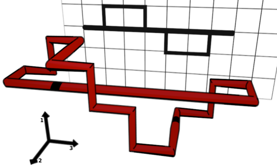
When restricting one of the SAWs to step only along the pulling direction axis, the resulting object shall be called a directed SAUK with axis. An example of such a directed SAUK with axis (which is also constrained according to the rules defined below) is shown in Figure 3.1. More precisely, choosing the lattice base vector $\hat{x}_{3}$ on the sc lattice and a root vertex $\varphi_{1}$ , we define a directed SAUK with axis $\varphi$ of length $n$ as a two component lattice object. The first component is a directed self-avoiding walk comprising of vertices $\varphi_{1},\,\varphi_{2},\,...\varphi_{m}$ such that

1. The walk ends on the axis defined by $\hat{x}_{3}$ and the root, i.e. $\varphi_{m}=\varphi_{1}+\left(n-m+1\right)\,\hat{x}_{3}$,

2. No vertex of the walk except $\varphi_{1}$ and $\varphi_{m}$ lie on the axis, i.e. $\varphi_{i}\neq\,\left(\varphi_{1}+j\,\hat{x}_{3}\right)$ for all $j\in\mathbb{N}$ and all $i=2,..,m-1$,

3. The walk is directed and makes no steps against the $\hat{x}_{3}$ direction, i.e. $\left(\varphi_{i+1}-\varphi_{i}\right)\cdot\hat{x}_{3}\geq 0$ for all $i=2,..,m-1$.

The second component is a walk of length $n-m$ that connects the vertices $\varphi_{m}$ and $\varphi_{1}$. The vertex positions are given as $\varphi_{i}=\varphi_{1}+\left(n-i+1\right)\,\hat{x}_{3}$ for all $i=m+1,...,n-1$.

We now construct a restricted directed SAUK with axis as follows. We consider a walk starting at the origin with initial steps $(-\hat{x}_{2})\hat{x}_{3}$. We then grow this walk by choosing to append steps to the final vertex as follows. We can append double steps $\hat{x}_{1}\hat{x}_{3}$ or $\left(-\hat{x}_{1}\right)\hat{x}_{3}$. Additionally, if the $x_{1}$-component of the final vertex is non-zero, we can also to append triple steps $(-\hat{x}_{2})(-\hat{x}_{2})\hat{x}_{3}$ or $\hat{x}_{2}\hat{x}_{2}\hat{x}_{3}$ if the $x_{2}$-component of the final vertex is equal to $1$ or $-1$, respectively. A walk constructed in such a way lies in the slab $-1\leq x_{2}\leq 1$. With every appended double or triple step, we also prepend a step $-\hat{x}_{3}$ to the starting vertex of the walk. Whenever a vertex with components $\left(0,\,-1,\,n_{3}\in\mathbb{Z}\right)$ is reached, we can generate a SAUK by appending a double step in $\hat{x}_{2}(-\hat{x}_{3})$. A lattice object constructed according to these rules is shown in Figure 3.1.

Considering the writhe formula (2.7) we see that when $x_{1}>0$ the double steps in $\hat{x}_{2}$-direction increase the writhe $w$ by $1$, and the double steps in $-\hat{x}_{2}$-direction decrease the writhe by $1$. When $x_{1}<0$, the writhe contributions are inverted. There is no other source of writhe. Note that the writhe of this simplified directed SAUK with axis is an even integer. We do not consider a pulling force, so that when we denote the number of these specified SAUKs with length $n$ and writhe $w$ by $C_{n\,w}$ the partition function reads

$$Z_{n}\left(\beta_{l}\right)=\sum_{w}C_{n\,w}e^{\beta_{l}w}.$$ (3.1)

We note that we here use $w=Wr$, in contrast to the simulations of the undirected SAUK, where it is advantageous to use $w=4Wr$.

To solve the model, we will obtain an expression for the generating function of restricted SAUKs with axis

$$\bar{a}\left(\beta_{l},\,z\right):=\sum_{n}Z_{n}\left(\beta_{l}\right)z^{n}$$ (3.2)

and analyse its singularities, since the closest singularity $z_{c}(\beta_{l})$ to the origin gives us the free energy as $f(\beta_{l})=-\log z_{c}(\beta_{l})$. The generating function involved here is an algebraic function and as such can only have poles and branch points as singularities. We will find that for one range of $\beta_{l}$ the closest singularity to the origin is given by a branch point, while for another region it is given by a simple pole. The changeover between these two regions gives a phase transition. In particular, for small $\beta_{l}$ where we expect a phase of low writhe, we find a branch point singularity and a temperature-independent free energy, which in turn implies $\langle w\rangle=o(n)$. On the other hand, for large $\beta_{l}$ we find a simple pole and a non-constant free energy, which implies $\langle w\rangle\sim Cn$ with temperature-dependent $C>0$.

The strategies for solving similar problems have been used for example in [34, 35]. In addition to the generating function 3.2, one introduces a generating function for unfinished SAUKs of length $n$, where $n$ counts the number of steps in the walk and in the axis. Denote by $a_{h}$ the generating function of unfinished SAUKs whose walk ends on the plane $x_{2}=-1$ at $x_{1}=h$. Correspondingly, when the walk ends on the plane $x_{2}=1$, we denote the generating function by $b_{h}$. Therefore, $\bar{a}\left(\beta_{l},\,z\right)=z\,a_{0}\left(\beta_{l},\,z\right)$. Define $y_{l}=\exp\left\{\beta_{l}\right\}$, and with

$$\Theta\left(x\right)=\begin{cases}1&x>0,\\ 0&x\leq 0,\end{cases}$$

define

$$H{}_{h}\left(y_{l}\right):=\left\{y_{l}^{-1}\,\Theta\left(h\right)+y_{l}\,\Theta\left(-h\right)\right\}.$$ (3.3)

Note that $H_{-h}=1/H_{h}$ (when $h\neq 0$) and $H_{0}\left(y_{l}\right)=0$. Then, the recursion relations for the generating functions read

$$a_{h}=z^{3}\left(\delta_{h,0}+a_{h+1}+a_{h-1}\right)+z^{4}\,H_{h}\,b_{h},$$ (3.4)

and

$$b_{h}=z^{3}\left(b_{h+1}+b_{h-1}\right)+z^{4}\,H_{-h}\,a_{h}.$$ (3.5)

The factors $z^{3}$ and $z^{4}$ correspond to double and triple steps, respectively. The additional factor of $z$ is associated with the additional reverse step on the axis. For $h=0$, the generating function $a_{0}$ also contains the initial configuration formed by three steps. The goal is to obtain $a_{0}$ and to get rid of all the $b_{h}$. Note that for $h\neq 0$ (3.4) can be inverted to give

$$b_{h}=z^{-4}\,H_{-h}\left\{a_{h}-z^{3}\left(a_{h+1}+a_{h-1}\right)\right\}.$$ (3.6)

For $\left|h\right|>1$, this can be used in (3.5) to obtain the bulk relation for $a_{h}$,

$$0=z^{6}a_{h-2}-2z^{3}a_{h-1}+\left(1+2\,z^{6}-z^{8}\right)a_{h}-2\,z^{3}a_{h+1}+z^{6}\,a_{h+2}.$$ (3.7)

This is a difference equation of order four for $a_{h}$. The general solution has the form $a_{h}=\sum_{i=1}^{4}C_{i}\lambda_{i}^{h}$, where $\lambda_{i}$ are the roots of the characteristic equation to (3.7). The series expansion of the solutions yields $\lambda_{1}=1/\lambda_{2}=z^{3}+z^{7}+z^{9}+O\left(z^{11}\right)$ and $\lambda_{3}=1/\lambda_{4}=z^{3}-z^{7}+z^{9}+O\left(z^{11}\right)$. The solutions with the alternating sign in the expansion are incompatible with a generating function (i.e. $Z_{n}>0$) so that the solution must take the form

$$a_{h}=C^{+}\lambda_{+}^{h}\Theta\left(h\right)+C^{-}\lambda_{-}^{h}\Theta\left(-h\right)$$ (3.8)

with

$$\lambda_{\pm}\left(z\right)=\frac{1}{2z^{3}}\left(1-z^{4}\mp R\left(z\right)\right),$$ (3.9)

where $R\left(z\right)=\sqrt{1-2z^{4}-4z^{6}+z^{8}}$ and $\lambda_{+}\lambda_{-}=1$. It follows from the series expansions that $\lambda_{+}$ applies for $h>0$ and $\lambda_{-}$ for $h<0$.

With $r=\sqrt{\frac{1}{3}\left\{3-\frac{2\ 6^{2/3}}{\left(-9+\sqrt{129}\right)^{1/3}}+\left(6\left(-9+\sqrt{129}\right)\right)^{1/3}\right\}}$ , the solution (3.8) has a square root singularity at

$$z_{b} = \frac{1}{2}\left(\sqrt{3+\frac{2}{r}-r^{2}}-1-r\right)$$

$$\approx 0.717.$$

Therefore $R\left(z_{b}\right)=0$ and $z_{b}$ can be associated with a low-writhe phase as described above. For $\left|h\right|>1$ the solution (3.8) holds for any $C^{+},\,C^{-}\neq 0$. To make the solution work at $\left|h\right|=1$, one requires two boundary conditions that include $a_{1}$ and $a_{-1}$. These are obtained by considering clock- and counterclockwise round trips around the axis. According to (3.4)

$$a_{-1}=a_{-1}\left(a_{-2},\,a_{0},\,b_{-1}\right).$$ (3.11)

This notation implies that $a_{-1}$ is expressed through $a_{-2},\,a_{0}$ and $\,b_{-1}$. One continues using the relations (3.4), (3.5) and (3.6) on the right-hand side of (3.11). For example, in the next step, use (3.5) to express $b_{-1}=b_{-1}\left(b_{0},\,b_{-2},\,a_{-1}\right)$. It follows an equation

$$a_{-1}=a_{-1}\left(a_{-2},\,a_{0},\,b_{0},\,b_{-2},a_{-1}\right).$$ (3.12)

Use (3.5) again to substitute for $b_{0}$ yielding $a_{-1}=a_{-1}\left(a_{-2},\,a_{0},\,b_{-1},\,b_{1},\,b_{-2},a_{-1}\right)$. Next, all $b_{h}$ can be expressed in terms of $a_{h}$. It follows
$a_{-1}=a_{-1}\left(a_{-2},\,a_{0},\,a_{-2},a_{-1},a_{1},a_{2},\,a_{-3},a_{-1}\right)$. Finally, with (3.4), $a_{0}$ is expressed through $a_{-1}$ and $a_{1}$ yielding the boundary condition

$$0 = z^{6}-z^{12}\left(1+y_{l}^{2}\right)-z^{6}a_{-3}-z^{3}\left(-2+z^{6}\right)a_{-2}$$ (3.13)

$$+\left(-1+z^{6}+z^{8}-z^{12}\left(1+y_{l}^{2}\right)\right)a_{-1}$$

$$-z^{6}\left(-1+z^{6}\right)\left(1+y_{l}^{2}\right)a_{1}-z^{9}y_{l}^{2}a_{2}.$$

The second boundary condition is obtained analogously by starting with $a_{1}=a_{1}\left(a_{2},\,a_{0},\,b_{1}\right)$. It reads

$$0 = z^{12}\left(1+y_{l}^{2}\right)-z^{6}y_{l}^{2}+z^{9}a_{-2}+z^{6}\left(-1+z^{6}\right)\left(1+y_{l}^{2}\right)a_{-1}$$ (3.14)

$$+\left(z^{12}+\left(1-z^{6}-z^{8}+z^{12}\right)y_{l}^{2}\right)a_{1}$$

$$+z^{3}\left(-2+z^{6}\right)y_{l}^{2}a_{2}+z^{6}y_{l}^{2}a_{3}.$$

When the Ansatz (3.8) is plugged into the boundary relations (3.13, 3.14), one may solve the equation system for $C^{\pm}$. With the expression for $a_{0}$ from (3.4) the generating function becomes

$$\bar{a}\left(z,\,y_{l}\right) = z\,a_{0}$$ (3.15)

$$= z^{4}\left(1+C^{-}\lambda_{-}^{-1}+C^{+}\lambda_{+}\right).$$ (3.16)

The denominator $D$ of $\bar{a}$ can be considered a function $D=D\left(\lambda_{+}\left(z\right),\,\lambda_{-}\left(z\right),\,z,\,y_{l}\right)$ the roots of which are the pole singularities of $\bar{a}$. However, $D\left(z\right)$ is a very complicated function of $z$, so it seems not possible to determine the roots of $D$ and thereby the free energy in the corresponding phases. Nevertheless, one may set $z=z_{b}$ and determine if there exist values $y_{l}^{\left(c\right)}$, so that $D\left(z=z_{b},\,y_{l}^{\left(c\right)}\right)=0$. This means that there exists a phase transition from the low-writhe phase into a phase associated with a pole singularity, which can be seen as a high-writhe phase. At $z=z_{b}$, $\lambda_{+}=\lambda_{-}=\left(1-z_{b}^{4}\right)/z_{b}^{3}$ and as a function of $y_{l}$, the denominator has the form

$$D\left(z=z_{b},\,y_{l}\right)=A_{0}\left(z_{b}\right)-A_{2}\left(z_{b}\right)y_{l}^{2}+A_{4}\left(z_{b}\right)y_{l}^{4},$$ (3.17)

where

$$A_{0}=4z_{b}^{18}\left(1+z_{b}^{2}-6z_{b}^{6}-z_{b}^{8}+z_{b}^{10}\right),$$ (3.18)

$$A_{2} = \left(1+z_{b}^{4}\right)\times$$ (3.19)

$$\left\{5-z_{b}^{4}\left(17+41z_{b}^{2}-18z_{b}^{4}-93z_{b}^{6}-87z_{b}^{8}+67z_{b}^{10}\right.\right.$$

$$\left.\left.+100z_{b}^{12}+z_{b}^{14}-54z_{b}^{16}-8z_{b}^{18}+7z_{b}^{20}\right)\right\},$$

and

$$A_{4}=z_{b}^{12}\left(-1+z_{b}^{2}\right){}^{4}\left(1+z_{b}^{2}\right){}^{2}\left(1+2z_{b}^{2}+3z_{b}^{4}\right).$$ (3.20)

The singularities closest to the origin are found when

$$y_{l}^{\pm}=\sqrt{\frac{A_{2}\pm\sqrt{A_{2}^{2}-4A_{0}A_{4}}}{2\,A_{4}}}.$$ (3.21)

These two solutions are reciprocal of each other, and hence $\beta_{l}^{\pm}=\log y_{l}^{\pm}$ differ only by a change of sign. We denote by $z_{c}^{\pm}\left(\beta_{l}\right)$ the pole singularities as a function of $\beta_{l}$ for which $z^{\pm}\left(\beta_{l}^{\pm}\right)=z_{b}$. At $\beta_{l}=0$ the system is in the low-writhe phase so that the free energy must take the form

$$f\left(\beta_{l}\right)=-\begin{cases}\log z_{c}^{-}\left(\beta_{l}\right)&\beta_{l}<\beta_{l}^{-},\\ \log\left(z_{b}\right)&\mbox{$\beta$}_{l}^{-}\leq\beta_{l}\leq\mbox{$\beta$}_{l}^{+},\\ \log z_{c}^{+}\left(\beta_{l}\right)&\beta_{l}>\beta_{l}^{+}.\end{cases}$$ (3.22)

Numerically, the values approximate to ($z_{b}=0.7167$)

$$\beta_{l}^{\pm} = \pm 1.4045.$$ (3.23)

We conclude that we have shown that weighting the writhe of restricted directed SAUK with axis induces a phase transition at a non-trivial value of $\beta_{l}$. By construction, the high torque phase is associated with SAUKs that wrap around their axis. By analysing the singularity of the free energy one can further show that the phase transition is a second-order transition with a jump-discontinuity in the second derivative.

4 Simulations

Self-avoiding lattice knots, including SAUKs have been treated via simulations in the lattice polymer literature before. Most notably in [28], the authors considered SAPs of lengths up to $2\times 10^{5}$ via Markov Chain Monte Carlo (MCMC) simulations, where (effectively) uncorrelated samples were generated with the two-point pivot algorithm. Via a knot detection algorithm, the samples could then be categorized by knot type. Their main result was that the scaling exponent associated with the radius of gyration appears to be invariant when the ensemble of SAP is restricted to a certain knot type. Such a result cannot be derived from the renormalization group, as the renormalization group transformation will in general not preserve the knot type.

In this section we want to consider the ensemble of unknotted SAP (SAUK) weighted by their writhe. However, we will not use the same approach as in [28] to sample states via MCMC. There are two reasons for this. First, when the writhe of SAPs is weighted, the ensemble is dominated by increasingly denser states for which the pivot algorithm becomes ineffective. Second, the ensemble becomes increasingly populated by knotted states, thus it becomes hard to sample effectively.

Instead, in this section we solve the model (2.9) via simulations with the Wang-Landau algorithm (WLA) [36] using a local move set that preserves the knot type. In this section, we use $w=4\,Wr$, which is an integer for a SAP on the sc lattice.

4.1 Algorithm and Data

We use a parallel version of the WLA as discussed for example in [37]. We initialize an unknotted, rooted SAP on the positive half-space of the sc lattice (without restriction to a slab geometry) and generate new states using the pull-moves [38] (excluding the end-move). The pull-moves certainly preserve the knot type of the SAP, however in contrast to the case of the SAW, to our knowledge, it is not proven that the pull moves are ergodic within the knot type. For some simulations we also used kink transport between random positions. Suppose the current state is $\varphi$, then we obtain a state $\varphi^{*}$ by applying a move to $\varphi$. In order to determine the writhe of $\varphi^{*}$, we rely on the formula (2.7). Therefore, we need to determine the linking number of the SAUK $\varphi$ with the pushed off unknot $\varphi+0.5\,\left(1,\,1,1\right)^{T}$. The linking number can be determined by considering the signed crossing in a projection. Suppose we project the SAUK into the $x_{2}$-$x_{3}$ plane, then all crossings will occur at potential crossing points of the form $p_{c}=\left(x_{2}+0.5,\,x_{3}+0.5\right)$, $x_{2},\,x_{3}\in\mathbb{Z}$. Therefore, every time a bond is added, the two potential crossing points are determined and the bonds are linked to these crossing points via pointers. When there are already bonds linked to the crossing point, we cycle through all perpendicular bonds (that correspond to the pushed off curve or vice versa) and compute the sum of signed crossing that the new bond produces with all the bonds that have already been linked. This corresponds to the change in linking number. The same procedure is performed once a bond is removed. This time however, the linking number changes by the negative of the sum of signed crossings produced by the bond. This algorithm was inspired by [39].

In order to determine the extension (2.8), we keep a list of integer $N_{V}\left[H\right]$, which count the number of vertices in the plane $x_{3}=H$. Then, every time a move removes a vertex $\varphi_{i}$ from one position, we update the list as $N_{V}\left[\left(\varphi_{i}\right)_{3}\right]\leftarrow N_{V}\left[\left(\varphi_{i}\right)_{3}\right]-1$. The list is modified accordingly when the vertex is placed onto its new position. Finally, every time a list update yields $N_{V}\left[H\right]=0$ for some $H$, we set the new extension $h=H$. We do the same when the population increases from $N_{V}\left[H\right]=0$.

At given length $n$, we use the WLA to produce estimates for the quantities

$$s_{w\,h}:=\log C_{w\,h}$$ (4.1)

and

$$s_{w}\left(\beta_{h}\right):=\log\left(\sum_{h}C_{w\,h}\,e^{\beta_{h}h}\right).$$ (4.2)

Here, estimates means that we obtain (4.1, 4.2) modulo a constant, including a statistical error and possibly a systematic error. In order to obtain the estimate for $s_{w}\left(\beta_{h}\right)$ for general $\beta_{h}$, rather than for $\beta_{h}=0$ , we modify the acceptance probability of the canonical WLA. Suppose the current state at time $t$ is $\varphi\left(t\right)$ and the state $\varphi^{*}$ is proposed. Denote writhe and extension of the current state by $w\left(t\right)$ and $h\left(t\right)$, respectively. For $\varphi^{*}$, denote these as $w^{*}$ and $h^{*}$, then, we accept $\varphi^{*}$ with the probability

$$P_{acc}=exp\left\{s_{w=w\left(t\right)}^{\left(est\right)}\left(\beta_{h}\,t\right)-s_{w=w^{*}}^{\left(est\right)}\left(\beta_{h},\,t\right)+\beta_{h}\cdot\left(h^{*}-h\left(t\right)\right)\right\}.$$ (4.3)

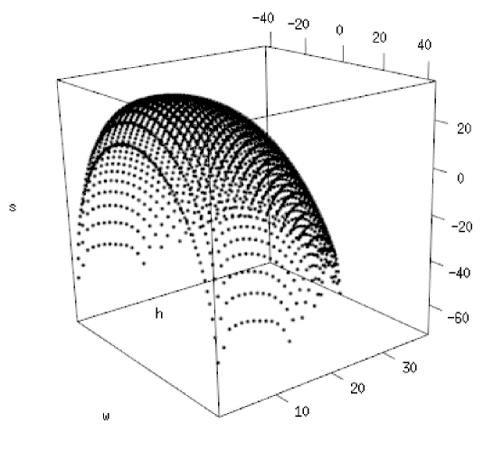
We ran multiple simulations to estimate $s_{n\,w}\left(\beta_{h}\right)$ at different lengths $n$ and stretching forces $\beta_{h}$. We actually produced estimates for $s_{n\,\left|w\right|}\left(\beta_{h}\right)$ and used the symmetry $s_{w}=s_{-w}$ to produce $s_{w}\left(\beta_{h}\right)$. We usually used a cut-off for the writhe, so that $\left|w\right|\leq 0.5\,n$. This can be justified because $s_{n\,w}\left(\beta_{h}\right)$ falls off quickly towards large $\left|w\right|$. This is for example shown in the estimate of the two-dimensional entropy at $n=80$ in Figure 4.1.

Figure 4.1: Two-dimensional entropy $s$ of the self-avoiding unknot at $n=80$ over the extension $h$ and the writhe $w=4\,Wr$. This entropy lacks macrostates $w>42$ as well as the macro state $\left(w=0,\,h=0\right)$. The problem of generating samples of planar polygons in three dimensions with the pull moves has been addressed in the appendix of [40].

The observables that we are interested in here are the derivatives of the free energy with respect to $\beta_{l}$. We denote the estimates of the derivatives by $f_{n}^{l}$, $f_{n}^{l\,l}$, $f_{n}^{l\,l\,l}$. Therefore,

$$f_{n}^{l}: = n^{-1}\left\langle w\right\rangle_{n}^{\left(est\right)},$$ (4.4)

$$f_{n}^{l\,l}: = n^{-1}\left\langle\left(w-\left\langle w\right\rangle^{\left(est\right)}\right)^{2}\right\rangle^{\left(est\right)},$$ (4.5)

$$f_{n}^{l\,l\,l} = n^{-1}\left(\left\langle w^{3}\right\rangle^{\left(est\right)}-3\left\langle w^{2}\right\rangle^{\left(est\right)}\left\langle w\right\rangle^{\left(est\right)}+2\,\left(\left\langle w\right\rangle^{\left(est\right)}\right)^{3}\right),$$ (4.6)

where for example $\left\langle w\right\rangle_{n}^{\left(est\right)}\left(\beta_{l},\,\beta_{h}=const\right)$ can be computed as

$$\left\langle w\right\rangle_{n}^{\left(est\right)}\left(\beta_{l},\,\beta_{h}=const\right)=\frac{\sum_{w}w\,e^{\beta_{l}\,w+s_{n\,w}^{\left(est\right)}\left(\beta_{h}\right)}}{\sum_{w}e^{\beta_{l}\,w+s_{n\,w}^{\left(est\right)}\left(\beta_{h}\right)}}.$$ (4.7)

We provide a $95\%$ confidence interval for our results, by obtaining from each simulation several estimates $s_{w}$ at different times. We choose the times long enough apart so that the estimates can be considered decorrelated. From each estimate, we compute observables, pretend them to be independent and compute the standard confidence interval.

We note while it is possible to consider other observables like the radius of gyration or the number of contacts by taking sample averages along $\varphi\left(t\right)$, we will not present such results here. We note that in particular good estimates for the radius of gyration will be good only for short lengths as the local move set requires a long time to decorrelate these observables. Also, since $\varphi\left(t\right)$ is not a Markov process, there is no (canonical) theory of the related error.

4.2 Results

Figure 4.2 shows writhe fluctuations $f_{n}^{ll}\left(\beta_{l},\,\beta_{h}\right)$ at length $n=80$. At $\beta_{h}\leq 0$, the maximum of the writhe fluctuation lies at $\beta_{l}=0$. As the pulling force is increased, the maximum splits into two modes, where the region between the peaks is expected to be dominated by states with many bonds aligned in force direction. This however suppresses the writhe fluctuations that occur along the polymer.

Figure 4.2: The graphic on the left-hand side shows a heat plot (rainbow colors) of the writhe fluctuations in the $\beta_{l}-\beta_{h}$-plane at length $n=80$. The fluctuations are maximal at the origin (violet-red). As $\beta_{h}$ is increased, this maximum begins to branch. This is also shown in the graphic on the right-hand side, which shows the writhe fluctuations per length at selected pulling forces $\beta_{h}$ against the torque $\beta_{l}$.

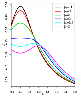
At a pulling force of approximately $\beta_{h}=2.5$, two peaks in $f_{n=80}^{ll}$ (Figure 4.2) appear. Note that this pulling force is small enough so that we do not have to worry about lattice effects from fully extended walks. In fact, the typical extension at $\beta_{l}=0,\,\beta_{h}=2.5$ is $\left\langle h\right\rangle_{n}/n\approx 0.25$ and thus about half of the possible maximum of $\left(h_{n}/n\right)^{\left(max\right)}=\left(n-2\right)/\left(2n\right)$. We will focus our analysis on $\beta_{h}=2.5$ which is an intermediate pulling force.

Figure 4.3: Scaling of the estimates of the first and second derivative of the free energy $f_{n}$ with respect to $\beta_{l}$ against $\beta_{l}$ at $\beta_{h}=2.5$.

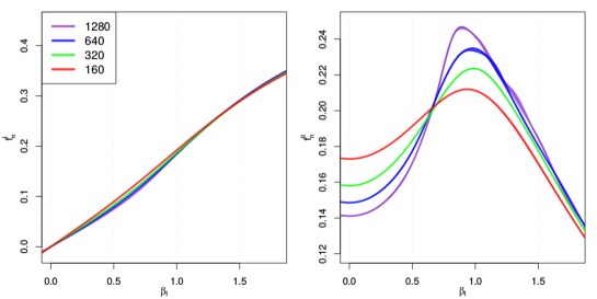
Figure 4.3 shows the scaling of the first and second derivative of the finite size free energy with respect to $\beta_{l}$ at $\beta_{h}=2.5$. While the scaling in the first derivative is rather weak, the peak in the second derivative grows with the length, however it is not clear whether it diverges. To investigate the nature of this transition further, we consider the third derivative.

Figure 4.4: Left graph: Scaling of the third derivative of the free energy with respect to $\beta_{l}$ at $\beta_{h}=2.5$. Right graph: Values of the maximum in $n\,f_{n}^{lll}\left(\beta_{h}=2.5\right)$ against the length in log-log-scale, together with a linear fit indicating a slope of $1.69(3)$.

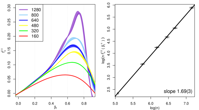
The third derivative is shown in the first graph of Figure 4.4. The second graph in Figure 4.4 shows a linear fit to the logarithm of the peak height in $n\,f_{n}^{lll}$ against the logarithm of the length. Using the standard scaling Ansatz 2.4 and differentiating three times with respect to $\tau$, we find that the third derivative, evaluated at the peak position, diverges as $f_{n}^{lll}\left(\beta_{l}^{\left(n\right)}\right)\sim n^{3\phi-1}$.

The good linear fit in Figure 4.4 suggests that this Ansatz is correct and we find $3\phi-1=0.69(3)$, and hence $\phi=0.56(2)$. While this indicates that the crossover exponent might be slightly larger than $1/2$, we have not taken corrections to scaling into account and hence don’t feel confident enough to exclude the value $\phi=1/2$.

4.3 Phase Diagram

Figure 4.5: Phase diagram in the force-torque plane. The red line marks a second-order phase transition. We cannot properly determine the position of the transition for small pulling forces.

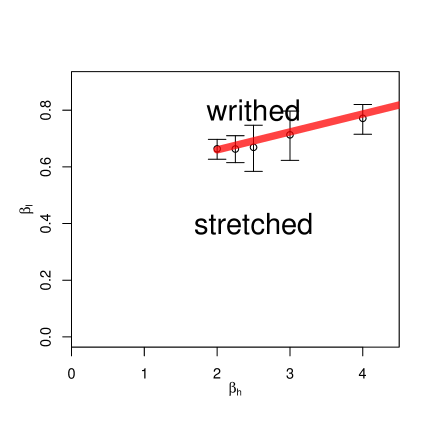
We use the peak position in the third derivative as a proxy for the location of the finite-size transition. We use $n=640$ as reference length and determine the location of the conjectured finite size transition to lie at $\beta_{l}^{640}\left(\beta_{h}=2.5\right)=0.67\left(8\right).$ The error corresponds to the torque $\beta_{l}$ range for which the confidence interval contains points that lie above the peak of its lower boundary. Also note that for $n\geq 480$, we do not observe any shift of the peak location $\beta_{l}^{\left(n\right)}\left(\beta_{h}=2.5\right)$, that lies outside the error. We obtained the locations of the transitions at different $\beta_{h}$ to obtain the phase diagram in Figure 4.5, where we have called the phase at high torque ’writhed’.

Figure 4.6: Scaling of the second derivative of the free energy with respect to $\beta_{l}$ at different pulling forces. At $\beta_{h}=0$, the graph shows the curves for the length $n=2580,\,1280,\,640,\,320$. One cannot make out clear scaling behavior. At $\beta_{h}=1$ the considered lengths are $n=1280,\,640,\,320$. There is weak non-trivial scaling so that the curve lowest at $\beta_{l}=0$ corresponds to $n=1280$ and the upper curve to $n=320$. At $\beta_{h}=2,\,4$ the lengths are $n=640,\,320,\,160$ and non-trivial scaling is apparent.

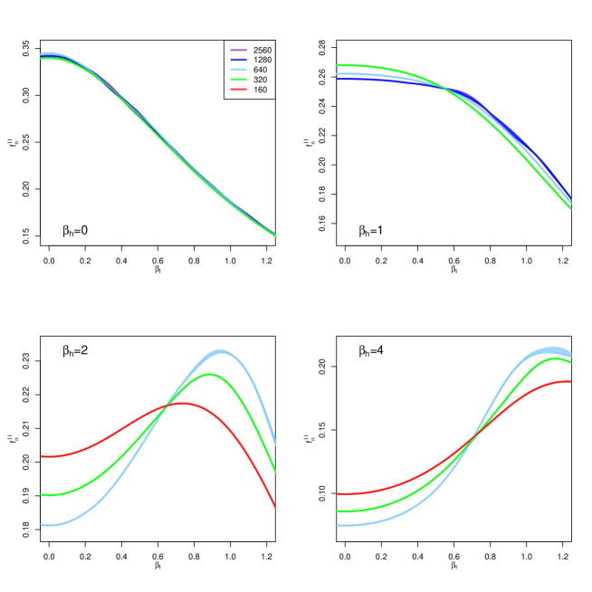
At values $\beta_{h}<2$ we were unable to obtain good estimates of the third derivative. Also, as $\beta_{h}$ decreases all signs of scaling fade out from the second derivative at the considered lengths, so that at $\beta_{h}=0$ the second derivative $f_{n}^{ll}$ appears to scale trivially. This can be seen in Figure 4.6 which shows the scaling of the second derivative at different pulling forces.

Returning to $\beta_{h}=0$ we report that we have considered lengths of up to $n=2560$ and found no scaling. We even probed (not well converged) length $n=5120$ and did not see any good indication that non-trivial scaling might start to show. It is likely that then there is no transition when $\beta_{h}=0$, after all, the pulling force needs to be positive to have stretched phase at high temperatures.

Hence, two scenarios present themselves. Firstly, the stretched to writhed transition exists for all non-zero positive values of $\beta_{h}$ and strong corrections to scaling inhibit our ability to detect the transition, or, secondly there exists a minimum value $\beta_{h}$ below which the transition does not exist.

Given the form of the writhe fluctuations being maximal around zero it is entirely possible that at small pulling force and short lengths the writhe fluctuations are dominated by a contribution that scales trivially and overpowers the leading non-trivial scaling term. We therefore conclude the first scenario is more likely. However, further work on this is clearly warranted.

5 Conclusion

In this paper we study an ensemble of unknotted self-avoiding polygons on the sc lattice weighted by writhe to identify potential phase transitions, as this can be related to experiments that turn DNA. We define and solve a simplified model for the strongly pulled regime, and show in this model the existence of a phase transition between phases of low and high writhe at a non-zero temperature.

We next consider the full problem using simulations with the Wang-Landau Algorithm. When the unknotted self-avoiding polygon is pulled sufficiently, we provide results that are compatible with a second-order phase transition between phases of low and high writhe. At low torques the unknotted self-avoiding polygon is in a stretched phase with anisotropic size scaling. As the pulling force is reduced, we observe that the scaling in the writhe fluctuations fades out, so that at zero pulling force $\beta_{h}=0$, we do not find any signs of scaling. It will be interesting to explore in further studies how the transition changes at low pulling forces.

References

- [1] T. Strick, J.-F. Allemand, V. Croquette, and D. Bensimon. Twisting and stretching single DNA molecules. Progress in Biophysics and Molecular Biology, 74(1-2):115 – 140, 2000.
- [2] T. R. Strick, Allemand J.-F., D. Bensimon, A. Bensimon, and V. Croquette. The elasticity of a single supercoiled DNA molecule. Science, 271(5257):1835, 1996.
- [3] S. B. Smith, L. Finzi, and C. Bustamante. Direct mechanical measurements of the elasticity of single DNA molecules by using magnetic beads. Science, 258(5085):1122–1126, 1992.
- [4] S. Forth, C. Deufel, M. Y. Sheinin, B. Daniels, J. P. Sethna, and M. D. Wang. Abrupt buckling transition observed during the plectoneme formation of individual DNA molecules. Physical Review Letters, 100:148301, 2008.
- [5] H. Brutzer, N. Luzzietti, D. Klaue, and R. Seidel. Energetics at the DNA supercoiling transition. Biophysical Journal, 98(7):1267, 2010.
- [6] C. Deufel, S. Forth, C. R. Simmons, S. Dejgosha, and M. D. Wang. Nanofabricated quartz cylinders for angular trapping: DNA supercoiling torque detection. Nature Methods, 4(3):223 – 225, 2007.
- [7] F. Mosconi, J. F. Allemand, D. Bensimon, and V. Croquette. Measurement of the torque on a single stretched and twisted DNA using magnetic tweezers. Physical Review Letters, 102(7):078301, 2009.
- [8] S. Sinha and J. Samuel. Statistical mechanics of ribbons under bending and twisting torques. Journal of Physics: Condensed Matter, 25(46):465102, 2013.
- [9] F. B. Fuller. Decomposition of the linking number of a closed ribbon: A problem from molecular biology. Proceedings of the National Academy of Sciences, 75(8):3557–3561, 1978.
- [10] S. Sinha and J. Samuel. Biopolymer elasticity: Mechanics and thermal fluctuations. Physical Review E, 85:041802, 2012.
- [11] J. Samuel and S. Sinha. Molecular elasticity and the geometric phase. Physical Review Letters, 90:098305, 2002.
- [12] J. Samuel and S. Sinha. Tops and writhing DNA. Journal of Statistical Physics, 143(2):399 – 412, 2011.
- [13] J. Samuel, S. Sinha, and A. Ghosh. Comment on "Writhe formulas and antipodal points in plectonemic DNA configurations". Physical Review. E, 80(6 Pt 1):063901; discussion 063902, 2009.
- [14] C. Bouchiat and M. Mezard. Elastic rod model of a supercoiled DNA molecule. The European Physical Journal E, 2(4):377–402, 2000.
- [15] J. H. White. Self-linking and the Gauss integral in higher dimensions. American Journal of Mathematics, 91(3):pp. 693–728, 1969.
- [16] G. Câlugâreanu. Sur les classes d’isotopie des noeuds tridimensionnels et leurs invariants. Czechoslovak Mathematical Journal, 11:588–625, 1961.
- [17] G. Câlugâreanu. Sur les enlacements tridimensionnels des courbes fermées. Communications of the Academia Republicii Populare Romîne, 11:829–832, 1961.
- [18] E. Janse van Rensburg, E. Orlandini, D. W. Sumners, M. C. Tesi, and S. G. Whittington Lattice ribbons: a model of double-stranded polymers. Physical Review E, 50:4279–4282, 1994.
- [19] E. Orlandini and E. Janse van Rensburg. Twist in an exactly solvable directed lattice ribbon. Journal of Statistical Physics, 80:781–791, 1995.
- [20] E. Dagrosa and A. L. Owczarek. Generalizing ribbons and the twist of the lattice ribbon. Journal of Statistical Physics, 155:392 – 417, 2014.
- [21] C. Vanderzande. Lattice models of polymers. Cambridge Lecture Notes in Physics, Vol. 11. Cambridge University Press, 1998.
- [22] A. Sokal. Critical exponents, hyperscaling, and universal amplitude ratios for two- and three-dimensional self-avoiding walks. Journal of Statistical Physics, 80(3-4):661, 1995.
- [23] N. Clisby. Accurate Estimate of the Critical Exponent for Self-Avoiding Walks via a Fast Implementation of the Pivot Algorithm. Physical Review Letters, 104(5):055702, 2010.
- [24] F. Valle, M. Favre, P. De Los Rios, A. Rosa, and G. Dietler. Scaling exponents and probability distributions of DNA end-to-end distance. Physical Review Letters, 95(15):158105, 2005.
- [25] K. DeBell and T. Lookman. Surface phase transitions in polymer systems. Reviews of Modern Physics, 65(1):87, 1993.
- [26] A. L. Owczarek, J. W. Essam, and R. Brak. Scaling analysis for the adsorption transition in a watermelon network of n directed non-intersecting walks. Journal of Statistical Physics, 102:997 – 1018, 2001.
- [27] E. J. J. Rensburg, E Orlandini, DW Sumners, M. C. Tesi, and S. G. Whittington. The Writhe of a self-avoiding polygon. Journal of Physics A: Mathematical and General, 26(19):L981 – L986, 1993.
- [28] M. Baiesi and E. Orlandini. Universal properties of knotted polymer rings. Physical Review E, 86(3-1):1 – 7, 2012.
- [29] C. Micheletti, D. Marenduzzo, E. Orlandini, and D. W. Summers. Knotting of random ring polymers in confined spaces. Journal of Chemical Physics, 124(6):064903, 2006.
- [30] M. Baiesi, E. Orlandini, and S. G. Whittington. Interplay between writhe and knotting for swollen and compact polymers. Journal of Chemical Physics, 131(15):154902, 2009.
- [31] M. Baiesi, E. Orlandini, and A. L. Stella. Ranking knots of random, globular polymer rings. Physical Review Letters, 99(5), 2007.
- [32] C. Laing and D. W. Sumners. Computing the writhe on lattices. Journal of Physics A: Mathematical and General, 39(14):3535, 2006.
- [33] E. Dagrosa. Statistical mechanics of twist-storing polymers. Dissertation, University of Melbourne, 2015.
- [34] J. Krawczyk, A. L. Owczarek, T. Prellberg, and A. Rechnitzer. Pulling absorbing and collapsing polymers from a surface. Journal of Statistical Mechanics: Theory and Experiment, 2005(05):P05008, 2005.
- [35] R. Brak, G. K. Iliev, A. L. Owczarek, and S. G. Whittington. The exact solution of a three-dimensional lattice polymer confined in a slab with sticky walls. Journal of Physics A: Mathematical and Theoretical, 43(13):135001, 2010.
- [36] F. Wang and D. P. Landau. Efficient, multiple-range random walk algorithm to calculate the density of states. Physical Review Letters, 86:2050–2053, 2001.
- [37] Y. W. Li, T. Vogel, T. Wuest, and D. P. Landau. A new paradigm for petascale Monte Carlo simulation: Replica exchange Wang-Landau sampling. Journal of Physics: Conference Series, 510(1):012012, 2014.
- [38] N. Lesh, M. Mitzenmacher, and S. Whitesides. A complete and effective move set for simplified protein folding. In Proceedings of the seventh annual international conference on Research in computational molecular biology, Recomb ’03, pages 188–195, New York, NY, USA, 2003. ACM.
- [39] R. C. Lacher and F. B. Sumners. Data structures and algorithms for computation of topological invariants of entanglements: Link, Twist, Writhe. In R.J.Roe, editor, Computer Simulation of Polymers, pages 365–373. Prentice-Hall, Englewood Cliffs, NJ, 1991.
- [40] A. Swetnam and C. Brett and M. P. Allen. Phase diagrams of knotted and unknotted ring polymers Physical Review E, 85:031804, 2012.