Axial-vector dominance predictions in quasielastic neutrino-nucleus scattering

Abstract

The axial form factor plays a crucial role in quasielastic neutrino-nucleus scattering, but the error of the theoretical cross section due to uncertainties of $G_{A}$ remains to be established. Reversely, the extraction of $G_{A}$ from the neutrino nucleus cross section suffers from large systematic errors due to nuclear model dependencies, while the use of single parameter dipole fits underestimates the errors and prevents an identification of the relevant kinematics for this determination. We propose to use a generalized axial-vector-meson-dominance (AVMD) in conjunction with large-$N_{c}$ and high energy QCD constrains to model the nucleon axial form factor, as well as the half width rule as an a priori uncertainty estimate. The minimal hadronic ansatz comprises the sum of two monopoles corresponding to the lightest axial-vector mesons being coupled to the axial current. The parameters of the resulting axial form factor are the masses and widths of the two axial mesons as obtained from the averaged PDG values. By applying the half width rule in a Monte Carlo simulation, a distribution of theoretical predictions can then be generated for the neutrino-nucleus quasielastic cross section. We test the model by applying it to the $(\nu_{\mu},\mu)$ quasielastic cross section from ¹²C for the kinematics of the MiniBooNE experiment. The resulting predictions have no free parameters. We find that the relativistic Fermi gas model globally reproduces the experimental data, giving $\chi^{2}/\#bins=0.81$. A $Q^{2}$-dependent error analysis of the neutrino data shows that the uncertainties in the axial form factor $G_{A}(Q^{2})$ are comparable to the ones induced by the a priori half width rule. We identify the most sensitive region to be in the range $0.2\lesssim Q^{2}\lesssim 0.6\,{\rm GeV}^{2}$.

I Introduction

Since the first measurement of the muon neutrino charged current quasielastic double differential cross section Agu08 ; Agu10 ; Agu13 many attempts have been made to characterize an effective axial-vector form factor of the nucleon Gal11 ; For12 ; Mor12 ; Alv14 . This is often made in terms of a dipole axial mass $M_{A}$, assuming a dipole form Nie12 ; But14 , for $Q^{2}>0$

$$G_{A}^{\rm dipole}(Q^{2}) = \frac{g_{A}}{(1+Q^{2}/M^{2}_{A})^{2}}\,.$$ (1)

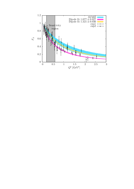
The world average value of the nucleon dipole axial mass is $M_{A}\sim 1$ GeV Liesenfeld:1999mv (see e.g. Ber02 for a review and references therein) which is obtained as a weighted sum of different oncoming dipole fits to independent experiments. However, this does not mean that the full spread of axial form factors can be described by a single dipole mass with a given uncertainty in a statistically significant way. Actually, there is a great variety of often largely incompatible experimental data from different processes which for illustration can be seen at Fig. 1. The correct discrimination and selection of these mutually compatible data is a complicated problem in data analysis which requires proper weighting of experimental ranges and falsifiable reliable theoretical input and not just parameterizations which awaits resolution and will not be addressed here. Nonetheless, given the present rather confusing state of affairs and the lack of further qualified information on what data on the axial form factor should one objectively prefer we will face the problem from a different and somewhat unconventional perspective where the traditional fitting strategy is sidestepped by the use of a theoretically based axial form factor with an inherent error band.

The MiniBooNE cross section data values are too large compared to the theoretical models of quasielastic neutrino scattering in the impulse approximation, unless a significant larger value of $M_{A}\sim 1.35$ GeV is employed in the nuclear axial current. Microscopic explanations of the large value of $M_{A}$ have been proposed based on ingredients involving nucleon spectral functions and multinucleon emission induced by short range correlations and meson exchange currents Mar10 ; Ama11 ; Nie12 . Recently studies with a monopole parameterization have been performed in Meg13 as well as nucleon mean field effective mass analyses of blurred electron scattering data Amaro:2015zja . In the absence of reliable theoretical uncertainty estimates, the disparate values obtained upon consideration of different nuclear effects can so far be regarded as a genuine source of systematic errors. Those turn out to be much larger than the alleged statistical uncertainties which, if taken literally, would lead to the most precise determination of the axial form factor to date in the range $Q^{2}\lesssim 2\,{\rm GeV}^{2}$. A careful statistical analysis has been undertaken more recently Wilkinson:2015gea and some tension among different data in different models has been reported.

The popular dipole form factor parameterization enjoys the pQCD result Carlson:1985zu asymptotically, $G_{A}\sim 1/Q^{4}$, but despite the phenomenological success for separate and independent experiments, it finds no further theoretical support at finite $Q^{2}$, nor does it describe all experiments globally with an acceptable $\chi^{2}$ value. Moreover, a one parameter fit such as the dipole form introduces an artificial bias linking high and low energies unnaturally and tightly; it is unclear if the statistical fluctuations inherited from the uncertainties in experimental neutrino-nucleus scattering data are faithfully represented by the corresponding fluctuations in the dipole mass. This is a well known issue in the statistical analysis of data since the goodness of fit and the parameter confidence level is based on estimating the probability that the proposed parameterization be the correct one, and this implies a mapping between data fluctuations and the fitting parameter fluctuations. To overcome this limitation a model independent analysis of axial form factor using dispersion relations under definite convergence assumptions and based on neutrino scattering was performed Bhattacharya:2011ah , with the expected finding that errors inferred from a dipole ansatz analysis may be underestimated. A duality based parameterization has been proposed searching for significant deviations to the widely used dipole form Bodek:2007ym . To be fair one should say that the neutrino scattering vs nucleon axial form factor is a kind of red herring; the significance of nuclear effects is claimed after a fit of the dipolar mass to the data is undertaken in which case astonishingly precise values for the dipolar mass are inferred (see e.g. Nie12 where extremely accurate values for $M_{A}$ are quoted). Since neutrino based determinations often imply certain and some times questionable assumptions, it is instructive to review other sources of information which at least do not rest on the same assumptions.

On a fundamental level, ab initio calculations allow a direct evaluation of the axial current matrix elements. The first lattice QCD determination of the axial form factor Liu:1992ab provided $M_{A}=1.03(5)\,{\rm GeV}$ in agreement with world average neutrino data at the time $M_{A}=1.032(36)\,{\rm GeV}$. However, subsequent calculations Capitani:1998ff yield $M_{A}=1.5\,{\rm GeV}$, a number which has recently been confirmed Alexandrou:2010hf for unphysical pion masses (about twice the physical value); the corresponding dipolar axial mass is larger than the experimental one, although there is some trend to agreement as the pion mass approaches the physical value. The role of excited states has been analyzed in a more recent lattice analysis Junnarkar:2014jxa confirming these results. In addition, Light cone QCD sum rules also overestimate the experimental dipole fit by $30\%$Braun:2006hz in the range $1<Q^{2}<4\,{\rm GeV}^{2}$, a trend checked by subsequent analyses Wang:2006su ; Erkol:2011qh and agreeing also with lattice calculations. While these QCD calculations are still subjected to many improvements, one should also recognize that they generate a family of axial nucleon form factors which fall within the experimental band which is wide enough to pose again the pertinent question on which are the correct ones within uncertainties. This situation makes an interesting case of lifting the conventional fitting strategy based on ad hoc parameterizations and incompatible data in favor of assuming a theoretically founded axial nucleon form factor with a credible uncertainty band generated by independent fluctuations and not directly based on the neutrino-nucleus data under discussion. In this paper we propose a simple scheme furnishing these requirements, see Section II, and provide a framework where the significance of different nuclear effects might be addressed.

On the more phenomenological hadronic level, the algebra of fields Lee:1967iu which yields field-current identities Lee:1967iv imply a generalized meson dominance which has proven as a convenient tool to analyze many important hadronic properties and most notably generalized vertex functions and hadronic form factors Frampton:1969ry . In the particular case of conserved currents, and more specifically axial-vector currents the general form of the form factor is expected to be a sum of infinitely many monopoles with isovector axial meson masses, whereas the pQCD result Carlson:1985zu yields $G_{A}\sim 1/Q^{4}$. The goodness of the Axial Vector Meson Dominance (AVMD) for the axial nucleon form factor was posed in Ref.Gari:1984qs by including the strong vertex corrections. However, meson dominance implies exchange of resonances which have a mass spectrum characterized by a mass and a width. Amazingly there is a theoretical limit where meson-dominance with narrow resonances is realized in QCD, namely the large $N_{c}$-limit introduced by ’tHootf and Witten long ago 'tHooft:1973jz ; Witten:1979kh ; within the large $N_{c}$ expansion mesons become stable particles. Their width-to-mass ratio is $\Gamma_{R}/M_{R}={\cal O}(1/N_{c})\sim 0.33$ which turns out to give the correct order of magnitude of the average experimental value 0.12(8) Masjuan:2012gc . The phenomenological implications of meson dominance within a large $N_{c}$ approach have been analyzed in Ref. Mas13 and, after natural uncertainty estimates based on the resonance width, a good description of experimental data and lattice results was achieved, with competitive accuracy.

Motivated by these theoretical insights, in the present paper we explore the large-$N_{c}$-inspired parameterization of the nucleon axial form factor Mas13 , see Section II, and explore the consequences of axial-vector dominance directly. We apply these findings to neutrino-nucleus scattering by starting with the simplest nuclear model, i.e., the relativistic Fermi gas, see Section III, which can be worked analytically. We do this without fitting any neutrino data in Section IV. This simple approach allows to address more clearly some important issues from a statistical point of view, and in particular to pin down the region of $Q^{2}$-values where the axial nucleon form factor fits are more sensitive to the existing neutrino-nucleus scattering data, see Section V. We finally summarize our results in Section VI.

II Axial-vector meson dominance and the axial form factor

Figure 1: The axial meson dominance band prediction is compared with the experimental data from the nucleon and with the dipole prediction bands of ref. Nie12 using the Fermi-Gas approximation and some relevant nuclear and reaction effects thereof. Experimental data are from refs. Nam70 ; Ben25 ; Fur70 ; Dom73 ; Joo76 (exp1) and Bak81 ; Mil82 ; Kit83 ; Kit90 (exp2). The axial form factor and the data are normalized to $F_{A}(0)=1$.

Figure 2: The axial meson dominance band prediction divided by the dipole parameterization for $M_{A}=1.014$ MeV as a function of the dimensionless variable $\xi=2/(1+\sqrt{1+4m_{N}^{2}/Q^{2}})$ defined in Ref. Bodek:2007ym . Experimental data are from refs. Nam70 ; Ben25 ; Fur70 ; Dom73 ; Joo76 (exp1) and Bak81 ; Mil82 ; Kit83 ; Kit90 (exp2). The form factors and data are normalized to one for $Q^{2}=0$.

Axial-Vector Meson Dominance (AVMD) was first introduced by Lee and Zumino Lee:1967iv into particle physics as a very natural generalization of the successful realization that Vector-Meson dominance explained the bulk of electromagnetic form factors. It simply states that the axial-vector current is given by the current field identity, which for just $u,d$ quarks reads

$$\vec{J}_{A}^{\mu}=\frac{1}{2}\bar{q}\gamma_{\mu}\gamma_{5}\vec{\tau}q=\sum_{A}f_{A}\partial^{\nu}\vec{A}_{\mu\nu}+\sum_{P}f_{P}\partial_{\mu}\vec{P}\,,$$ (2)

where $f_{A}$ and $f_{P}$ are the decay amplitudes of the axial-vector $A=a_{1},a_{1}^{\prime},\dots$ and pseudoscalar mesons $P=\pi,\pi^{\prime},\dots$ respectively and $\vec{A}_{\mu\nu}=\partial_{\mu}\vec{A}_{\nu}-\partial_{\nu}\vec{A}_{\mu}$ is the corresponding field strength tensor of the axial meson. This equation yields a generalized PCAC, which implies in turn a generalization Dominguez:1971zg ; Dominguez:1971hf ; Dominguez:1976ut ; Dominguez:1977nt ; Dominguez:1977en ; Dominguez:1984ka of the celebrated Goldberger-Treimann relation.

As a consequence the axial form factor of the nucleon can be written as a sum of monopole form factors,

$$G_{A}(Q^{2})=g_{A}\sum_{n}c_{n,a}\frac{m_{n,a}^{2}}{m_{n,a}^{2}+Q^{2}}$$ (3)

where $c_{n,a}=f_{n,a}g_{n,aNN}/g_{A}$ and $f_{n,a}$, $g_{n,aNN}$ and $m_{n,a}$ are the vacuum amplitude, the coupling to the nucleon and the mass respectively of the corresponding isovector-axial-vector meson $n$. From $G_{A}(0)=g_{A}$ we have the normalization condition

$$1=\sum_{n}c_{n,a}\,.$$ (4)

The asymptotic pQCD result Carlson:1985zu , $G_{A}\sim 1/Q^{4}$, requires

$$0=\sum_{n}c_{n,a}m_{n,a}^{2}\,.$$ (5)

In this paper we use the minimal hadronic ansatz for axial nucleon form factor furnishing meson dominance and proper pQCD behavior

$$G_{A}(Q^{2})=g_{A}F_{A}(Q^{2})=g_{A}\frac{m^{2}_{a_{1}}m^{2}_{a^{\prime}_{1}}}{(m^{2}_{a_{1}}+Q^{2})(m^{2}_{a^{\prime}_{1}}+Q^{2})}$$ (6)

with $g_{A}=1.267$, and where the axial meson masses are $m_{a_{1}}=1.230$ GeV, $m_{a^{\prime}_{1}}=1.647$ GeV. As noted in Ref. Mas13 one of the problems with this ansatz is that generally the interpolating fields are resonances which have a mass and a width, and we stand by the solution proposed there to use the width as a genuine uncertainty of the meson dominance ansatz. This generates a full band of predictions which provide an uncertainty range for a formula of the form of Eq. (6). The experimental widths are $\Gamma_{a_{1}}=0.425$ GeV, and $\Gamma_{a^{\prime}_{1}}=0.254$ GeV as listed in the PDG compilation Beringer:1900zz  . The masses are only the central values of the axial mesons spectra. We use the half-width rule to generate random values for $m_{a_{1}}$ and $m_{a^{\prime}_{1}}$ following Gaussian distributions with variances $\Gamma_{a_{1}}/2$ and $\Gamma_{a_{1}^{\prime}}/2$ respectively. This provides a distribution band for the axial form factor Mas13 which is slightly above the bulk of the abundant and incompatible $G_{A}$ data, see Fig. 1, but agrees well with the lattice  Capitani:1998ff ; Alexandrou:2010hf ; Junnarkar:2014jxa and light cone QCD sum rules estimates Braun:2006hz ; Wang:2006su ; Erkol:2011qh .

It might be useful to provide a parameterization of the uncertainty bands of the AVMD form factor as $F_{A}^{\rm lower}(Q^{2})\leq F_{A}(Q^{2})\leq F_{A}^{\rm upper}(Q^{2})$. The lower and upper axial form factors are defined as the boundaries of the usual $1\sigma$ 68% confidence level region. They can be parameterized as a product of two monopoles, similarly to Eq. (6), as

$$F_{A}^{\alpha}(Q^{2})=\frac{\Lambda^{2}_{\alpha}\Lambda^{2}_{\alpha^{\prime}}}{(\Lambda^{2}_{\alpha}+Q^{2})(\Lambda^{2}_{\alpha^{\prime}}+Q^{2})}$$ (7)

with $\alpha=\rm upper\,,lower$. By a fit in the range $0\leq Q^{2}\leq 3\,\rm GeV^{2}$, corresponding to the blue band of Fig.1, the cut-off parameters turn out to be $(\Lambda_{\rm lower},\Lambda_{\rm lower^{\prime}})=(0.97486,1.73345)$, and $(\Lambda_{\rm upper},\Lambda_{\rm upper^{\prime}})=(1.5436,1.54194)$, respectively (in GeV) . These values illustrate the fact that the fluctuations of the form factor do not necessarily correspond to a single dipole mass fluctuation.

We will thus apply this axial form factor band for the neutrino cross section theoretical predictions. Our point of view is that given the many effects which might contribute to neutrino-nucleus scattering it may be sensible to use a credible form factor with an error estimate based on a different source of data, without resting on a specific fit to the neutrino data. It was found in Ref. Mas13 that the large-$N_{c}$ meson dominated form factors with pQCD constraints and supplemented with the half-width rule for an uncertainty estimate worked well also for other form factors such as electromagnetic, scalar and gravitational form factors. As a general rule uncertainties turned out to be comparable or smaller than lattice QCD predictions but larger than experimental data.

After presenting our main results, for completeness we will also analyze the conventional approach of fitting Eq. (6) to the MiniBoone data. We want to investigate the traditional point of view of assuming certain nuclear effects before undertaking a fit of the axial form factor of the nucleon. For example in Ref. Nie12 a model with nucleon spectral functions, RPA correlations and MEC has been considered and a fit to the axial form factor has been undertaken assuming a fixed $\Delta-N$-transition form factor. We want to understand why in these studies one can extract more accurate information on the axial form factor than on the nuclear model response functions.

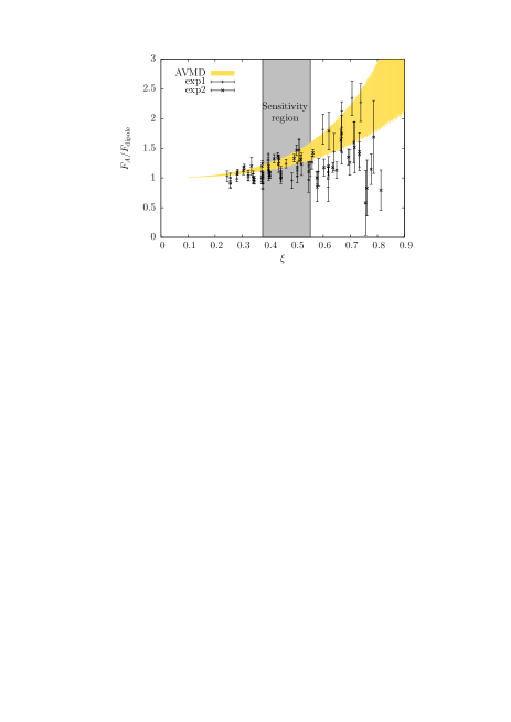
Anticipating some of the results to be discussed below, and for a comparison we depict also in Fig. 1 the results found in the analysis of  Nie12 where the role of nuclear effects beyond the local Fermi-Gas have been addressed when a dipole form factor is fitted to the neutrino scattering data. As can be deduced from Fig. 1 the statistical errors are comparable when including the additional nuclear effects and the large and quite visible systematic change between the two fits is comparable to the spread generated by our AVMD form factor. Following the scheme of Ref. Bodek:2007ym we also plot in Fig. 2 the ratio between the AVMD form factor and the dipole form factor, Eq. (1), with $M_{A}=1.014\,{\rm GeV}$ in terms of the dimensionless variable $\xi$ defined there. This quotient was fitted in  Bodek:2007ym by including an interpolating polynomial without discarding any of the compiled data which, as we have mentioned, are incompatible as a whole . As we can see the AVMD model produces a spread compatible with the spread of the region covered by the form factor data.

In both Fig. 1 and Fig. 2 we also highlight in shaded gray the main $Q^{2}$ region where fluctuations in the axial form factor have a sizable impact in the MiniBooNE data, as will be discussed below in Section V. Thus, our AVMD motivated axial form factor describes reasonably well the known data spread in the $Q^{2}$-region relevant for the MiniBooNE experiment.

III Quasielastic neutrino scattering

In this paper we are interested in the charged-current quasielastic (CCQE) reactions in nuclei induced by neutrinos. In particular we compute the $(\nu_{\mu},\mu^{-})$ cross section. The total energies of the incident neutrino and detected muon are $\epsilon=E_{\nu}$, $\epsilon^{\prime}=m_{\mu}+T_{\mu}$, and their momenta are ${\bf k},{\bf k}^{\prime}$. The four-momentum transfer is $k^{\mu}-k^{\prime}{}^{\mu}=(\omega,{\bf q})$, with $Q^{2}=q^{2}-\omega^{2}>0$. If the lepton scattering angle is $\theta$, the double-differential cross section can be written as Ama05a ; Ama05b

$$\frac{d^{2}\sigma}{dT_{\mu}d\cos\theta}(E_{\nu})=\left(\frac{M_{W}^{2}}{M_{W}^{2}+Q^{2}}\right)^{2}\frac{G^{2}\cos^{2}\theta_{c}}{4\pi}\frac{k^{\prime}}{\epsilon}v_{0}S_{\pm}$$ (8)

Here $G=1.166\times 10^{-11}\quad\rm MeV^{-2}\sim 10^{-5}/m_{p}^{2}$ is the Fermi constant, $\theta_{c}$ is the Cabibbo angle, $\cos\theta_{c}=0.975$, and the kinematical factor $v_{0}=(\epsilon+\epsilon^{\prime})^{2}-q^{2}$.

The nuclear structure function $S_{\pm}$ is defined as a linear combination of the five nuclear response functions (+ is for neutrinos and $-$ is for antineutrinos)

$$S_{\pm}=V_{CC}R_{CC}+2{V}_{CL}R_{CL}+{V}_{LL}R_{LL}+{V}_{T}R_{T}\pm 2{V}_{T^{\prime}}R_{T^{\prime}}\ ,$$ (9)

where the $V_{K}$ coefficients depends only on the neutrino and muon kinematics and do not depend on the details of the nuclear target.

$${V}_{CC} = 1-\delta^{2}\frac{Q^{2}}{v_{0}}$$ (10)

$${V}_{CL} = \frac{\omega}{q}+\frac{\delta^{2}}{\rho^{\prime}}\frac{Q^{2}}{v_{0}}$$ (11)

$${V}_{LL} = \frac{\omega^{2}}{q^{2}}+\left(1+\frac{2\omega}{q\rho^{\prime}}+\rho\delta^{2}\right)\delta^{2}\frac{Q^{2}}{v_{0}}$$ (12)

$${V}_{T} = \frac{Q^{2}}{v_{0}}+\frac{\rho}{2}-\frac{\delta^{2}}{\rho^{\prime}}\left(\frac{\omega}{q}+\frac{1}{2}\rho\rho^{\prime}\delta^{2}\right)\frac{Q^{2}}{v_{0}}$$ (13)

$${V}_{T^{\prime}} = \frac{1}{\rho^{\prime}}\left(1-\frac{\omega\rho^{\prime}}{q}\delta^{2}\right)\frac{Q^{2}}{v_{0}}.$$ (14)

where we have defined the dimensionless factors $\delta=m^{\prime}/\sqrt{Q^{2}}$, proportional to the muon mass $m^{\prime}$, $\rho=Q^{2}/q^{2}$, and $\rho^{\prime}=q/(\epsilon+\epsilon^{\prime})$.

We evaluate the five nuclear response functions $R_{K}$, $K=CC,CL,LL,T,T^{\prime}$ ($C$=Coulomb, $L$=longitudinal, $T$=transverse). following the simplest approach that treats exactly relativity, gauge invariance and translational invariance, that is the relativistic Fermi gas model (RFG) Ama05a ; Ama05b . The single nucleons are described by plane wave spinors and the response functions are analytical. It is a remarkable result that the nuclear response function $R_{K}$ of the RFG is proportional to a single-nucleon response function $U_{K}$ times the so-called scaling function $f(\psi)$

$$R_{K}=\frac{N\xi_{F}}{m_{N}\eta_{F}^{3}\kappa}U_{K}f(\psi)$$ (15)

where $N$ is the neutron number, $\eta_{F}=k_{F}/m_{N}$, and $\xi_{F}=\sqrt{1+\eta_{F}^{2}}-1$. The scaling function is defined as

$$f(\psi)=\frac{3}{4}(1-\psi^{2})\theta(1-\psi^{2})$$ (16)

where $\theta$ is the Heavyside step function and $\psi$ is the scaling variable

$$\psi^{2}=\frac{1}{\xi_{F}}{\rm max}\left\{\kappa\sqrt{1+\frac{1}{\tau}}-\lambda-1,\xi_{F}-2\lambda\right\}$$ (17)

where $\lambda=\omega/(2m_{N})$, $\kappa=q/(2m_{N})$, and $\tau=\kappa^{2}-\lambda^{2}$.

Finally, we give the single-nucleon responses $U_{K}$. For $K=CC$ it is the sum of vector and axial-vector response, in turns written as the sum of conserved (c.) plus non conserved (n.c.) parts,

$$U_{CC} = U_{CC}^{V}+\left(U_{CC}^{A}\right)_{\rm c.}+\left(U_{CC}^{A}\right)_{\rm n.c.}$$ (18)

For the vector CC response we have

$$U_{CC}^{V} = \frac{\kappa^{2}}{\tau}\left[(2G_{E}^{V})^{2}+\frac{(2G_{E}^{V})^{2}+\tau(2G_{M}^{V})^{2}}{1+\tau}\Delta\right]\ ,$$ (19)

where $G_{E}^{V}$ and $G_{M}^{V}$ are the isovector electric and magnetic nucleon form factors (we use Galster’s parameterization), and

$$\Delta=\frac{\tau}{\kappa^{2}}\xi_{F}(1-\psi^{2})\left[\kappa\sqrt{1+\frac{1}{\tau}}+\frac{\xi_{F}}{3}(1-\psi^{2})\right].$$ (20)

The axial-vector CC response is the sum of conserved (c.) plus non conserved (n.c.) parts,

$$\left(U_{CC}^{A}\right)_{\rm c.} = \frac{\kappa^{2}}{\tau}G_{A}^{2}\Delta$$ (21)

$$\left(U_{CC}^{A}\right)_{\rm n.c.} = \frac{\lambda^{2}}{\tau}(G_{A}-\tau G_{P})^{2}.$$ (22)

where $G_{A}$ is the nucleon axial-vector form factor and $G_{P}$ the pseudoscalar axial form factor. From PCAC the pseudoscalar form factor is

$$G_{P}=\frac{4m_{N}^{2}}{m_{\pi}^{2}+Q^{2}}G_{A}.$$ (23)

Similarly, for $K=CL,LL$ we have

$$U_{CL} = U_{CL}^{V}+\left(U_{CL}^{A}\right)_{\rm c.}+\left(U_{CL}^{A}\right)_{\rm n.c.}$$ (24)

$$U_{LL} = U_{LL}^{V}+\left(U_{LL}^{A}\right)_{\rm c.}+\left(U_{LL}^{A}\right)_{\rm n.c.}\ ,$$ (25)

The vector and conserved axial-vector parts are determined by current conservation

$$U_{CL}^{V} = -\frac{\lambda}{\kappa}U_{CC}^{V}$$ (26)

$$\left(U_{CL}^{A}\right)_{\rm c.} = -\frac{\lambda}{\kappa}\left(U_{CC}^{A}\right)_{\rm c.}$$ (27)

$$U_{LL}^{V} = \frac{\lambda^{2}}{\kappa^{2}}U_{CC}^{V}$$ (28)

$$\left(U_{LL}^{A}\right)_{\rm c.} = \frac{\lambda^{2}}{\kappa^{2}}\left(U_{CC}^{A}\right)_{\rm c.}\ ,$$ (29)

while the n.c. parts are

$$\left(U_{CL}^{A}\right)_{\rm n.c.} = -\frac{\lambda\kappa}{\tau}(G_{A}-\tau G_{P})^{2}$$ (30)

$$\left(U_{LL}^{A}\right)_{\rm n.c.} = \frac{\kappa^{2}}{\tau}(G_{A}-\tau G_{P})^{2}\ .$$ (31)

Finally the transverse responses are given by

$$U_{T} = U_{T}^{V}+U_{T}^{A}$$ (32)

$$U_{T}^{V} = 2\tau(2G_{M}^{V})^{2}+\frac{(2G_{E}^{V})^{2}+\tau(2G_{M}^{V})^{2}}{1+\tau}\Delta$$ (33)

$$U_{T}^{A} = 2(1+\tau)G_{A}^{2}+G_{A}^{2}\Delta$$ (34)

$$U_{T^{\prime}} = 2G_{A}(2G_{M}^{V})\sqrt{\tau(1+\tau)}[1+\tilde{\Delta}]$$ (35)

with

$$\tilde{\Delta}=\sqrt{\frac{\tau}{1+\tau}}\frac{\xi_{F}(1-\psi^{2})}{2\kappa}\ .$$ (36)

IV Numerical results

In Fig.3 we show the AVMD predictions for the total integrated CCQE cross section

$$\sigma(E_{\nu})=\int dT_{\mu}\int d\cos\theta\frac{d^{2}\sigma}{dT_{\mu}d\cos\theta}(E_{\nu}).$$ (37)

The theoretical uncertainties represented by the displayed band have been computed by a Monte Carlo calculation assuming a Gaussian distribution for the axial meson mass distributions. For comparison we show also the results obtained with a dipole axial form factor with $M_{A}=1$ GeV. The MiniBooNE data are compatible with the axial meson-dominance predictions. Note that no attempts to fit the experimental data have been made. The only parameter of the RFG model is the Fermi momentum $k_{F}=225$ MeV.

Figure 3: Integrated quasielastic neutrino cross section of ¹²C. The axial meson dominance band prediction is centered around the axial meson masses, and it is compared to the dipole parameterization with dipolar axial mass $M_{A}=1$ GeV. The experimental data are from MiniBooNE experiment.

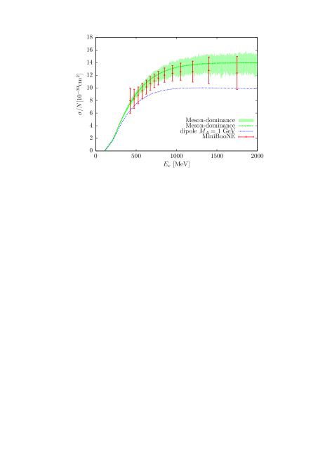
The MiniBooNE unfolded energy dependent cross section is model dependent based on a reconstruction of the neutrino energies assuming a quasielastic interaction with a neutron at rest. These data suffer from uncertainties driven by the model dependence of the neutrino energy reconstruction. For proper and useful comparisons, the flux-averaged doubly differential cross section should be used. We compute this cross section as

$$\frac{d^{2}\sigma}{dT_{\mu}d\cos\theta}=\frac{\int dE_{\nu}\phi(E_{\nu})\frac{d^{2}\sigma}{dT_{\mu}d\cos\theta}(E_{\nu})}{\int dE_{\nu}\phi(E_{\nu})}$$ (38)

where $\phi(E_{\mu})$ is the incident neutrino flux.

Figure 4: Flux-averaged doubly differential CCQE cross section as a function of the muon kinetic energy. The continuous band predictions (green) have been computed for fixed values of $\cos\theta$ at the center of the experimental bins. The discrete meson dominance predictions have been computed by integrating the doubly-differential cross section over each discrete bin.

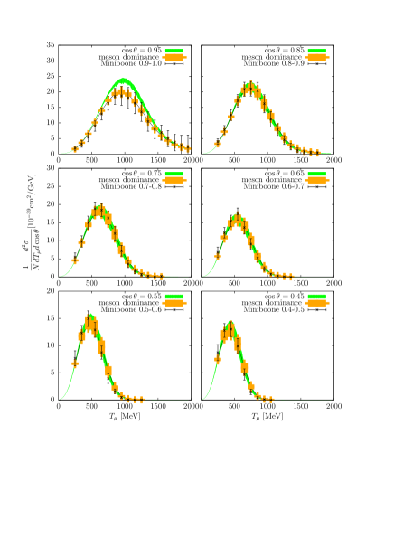
In figure 4 we show results for the flux-averaged doubly differential CCQE cross section as a function of the muon kinetic energy. The bands are the axial meson-dominance model predictions for fixed values of $\cos\theta$ at the center of the experimental bins.

Figure 5: Flux-averaged doubly differential CCQE cross section for several values of $\cos\theta$, and for low scattering angles, compared with the experimental data for the bin $\cos\theta=0.9$-1.0.

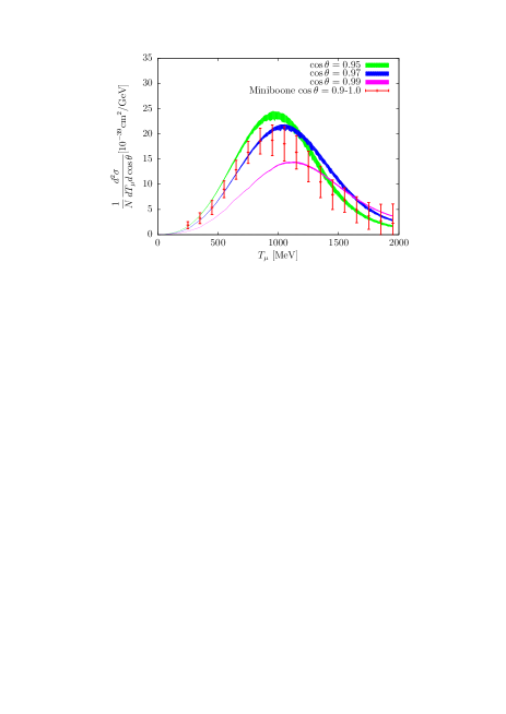
The MiniBooNE $\nu_{\mu}$ CCQE flux-integrated double differential cross section is provided in bins $(t_{i},t_{i+1})$ of $T_{\mu}$ and bins $(c_{j},c_{j+1})$ of $\cos\theta$. The size of the bins is $c_{j+1}-c_{j}=\Delta c=\Delta\cos\theta_{\mu}=0.1$, and $t_{i+1}-t_{i}=\Delta t=\Delta T_{\mu}=0.1$ GeV.

For a meaningful comparison with the experimental data we have computed the averaged cross section for each bin, by integrating the doubly-differential cross section over each discrete bin.

$$\Sigma_{ij}=\frac{1}{\Delta t\Delta c}\int_{t_{i}}^{t_{i+1}}dT_{\mu}\int_{c_{j}}^{c_{j+1}}d\cos\theta\frac{d^{2}\sigma}{dT_{\mu}d\cos\theta}.$$ (39)

Figure 6: The $\chi_{ij}$ computed values for each bin pair are represented in the $(\cos\theta_{\mu},T_{\mu})$ plane as a color image.

The axial vector dominance predictions for the averaged cross section $\Sigma_{ij}$ are also shown in figure 4, where they are compared to the experimental data. The theoretical errors are again computed by assuming a Gaussian distribution of the axial meson masses. Note that the averaged cross section for low scattering angles, bin $\cos\theta=0.9$-1.0, is quite different from the cross section at the central value $\cos\theta=0.95$. This is due to the strong angular dependence of the differential cross section for small angles, as can be seen in Fig. 5. Therefore the integration of the cross section over the bin is crucial to get the correct average. Note also that in this region the momentum transfer takes the smallest values compatible with energy transfer, and one expects that the model dependence of the results be maximized. As a matter of fact according to Ref. Amaro:2006tf the shell structure effects for both discrete and continuum are essentially washed out in favor of the RFG. For larger scattering angles, the angular dependence is mild, and the value of the cross section at the center of the bin is closer to the average, Eq. (39), as can be seen in Fig. 4.

V Goodness of the model

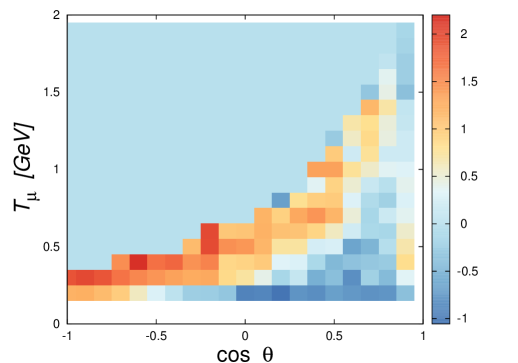
To get a global measure of the goodness of the theoretical model in describing the experimental data requires including both theoretical and experimental uncertainties. We thus compute the distance of theory to data as given by a $\chi^{2}$ metric, defined as $\chi^{2}=\sum_{i,j}\chi_{ij}^{2}$. The $\chi_{ij}$ matrix provides the distance between theory and experiment within each bin $(i,j)$, in units of the total uncertainty. It is defined as

$$\chi_{ij}=\frac{\Sigma_{ij}^{(th)}-\Sigma_{ij}^{(exp)}}{\sqrt{(\Delta\Sigma_{ij}^{(th)})^{2}+(\Delta\Sigma_{ij}^{(exp)})^{2}}}$$ (40)

where $\Delta\Sigma_{ij}^{(exp)}$ is the experimental error. and $\Delta\Sigma_{ij}^{(th)}$ is the theoretical uncertainty due to the physical widths of the axial mesons. In Fig. 6 we show the matrix values $\chi_{ij}$ computed for all the bins of the MiniBooNE CCQE neutrino experiment. We obtain $\chi^{2}=111$, so that dividing by the number of bins $N=137$, we get $\chi^{2}/N=0.81$. Globally the model agrees remarkably well with data taking into account that we do not minimize any $\chi^{2}$ and we just compute it.

While the $\chi^{2}$ value seems to be acceptable, let us analyze the assumptions underlying the comparison and its statistical significance in some more detail. We are just testing that the difference between the theory and the data should behave as a random variable, namely a standardized normal distribution. However, a look to the Fig. 6 reveals that the level of disagreement is located at the edges of the plot, while we should expect a more uniform pattern globally if the $\chi_{ij}$ were distributed randomly. This can be further elucidated by analyzing the differences. We find that there is a strong asymmetry in the residuals $\chi_{ij}$, indicating gross systematic differences. Thus, we believe that these large discrepancies are possibly beyond the applicability of the RFG. At the same time one should also admit that the double binning procedures, essential for a proper comparison with the data, tend to wash out nuclear effects.

As we anticipated in our discussion around Fig. 1 some fits to the dipolar axial mass do generate rather good $\chi^{2}$ values and unprecedented accuracy for the axial form factor Nie12 . Let us remind that, a too low value is as bad as a too high value, since the $\chi^{2}$-distribution for a large number of degrees of freedom $\nu=N-P$ behaves as a Gaussian distribution and thus it must be $\chi^{2}/\nu=1\pm\sqrt{2/\nu}$ within $1\sigma$ confidence level. For instance in Ref. Nie12 a value of $\chi^{2}/\nu=33/(137-2)=0.24$ was obtained which is outside the expected confidence level by $6\sigma$. This suggest that experimental errors may be too large, and the question is whether errors can be reduced without destroying the Gaussian nature of the fluctuations. Moreover, let us remind that the statistical approach based on $\chi^{2}$-fits deals with testing the validity of a given functional form for the true form factor, while despite the much extended popularity there is no field theoretical support for a dipole form factor.

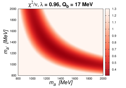
In order to understand those results we have performed a conventional $\chi^{2}$-fit with two axial masses as minimization parameters. For this fit we include only the experimental errors in the denominator of Eq. (40). As in Ref. Nie12 we normalize the data by a factor $\lambda=0.96$ and subtract a constant $Q$ -value $Q_{b}=17$ MeV to the energies of the particle-hole excitations (note that while this modification by hand of the RFG energies improves the fit, the gauge invariance of the model is broken). We find the minimum at $m_{a_{1}}=m_{a_{1}^{\prime}}=1293$ with $\chi^{2}/\nu=0.31$. We have tested the normality of residuals, and we find that they very likely correspond to a Gaussian distribution. This indicates that the experimental errors should probably be re-scaled by a factor less than $1/2$, i.e., the fit would be acceptable if the errors were twice smaller than stated in the experiment. This observation concerns all previous determinations of the dipolar axial mass from these neutrino data, based on fits trying to minimize the discrepancies with the experiment. Note that we are not disputing the existence of certain well known important nuclear effects. The total uncertainty on the theoretical neutrino-nucleus cross section can be due to uncertainties on both the nuclear effects and on the axial form factor. Here we focus on the size of the axial form factor uncertainties since they are obviously not small.

In Fig. 7 we plot the $\chi^{2}/\nu$ values as a function of the two axial masses, showing that they are highly correlated. While the dipole form factor (two equal axial masses) is contained in the confidence region around the minimum, it is not the only allowed solution as two different axial masses also provide acceptable fits.

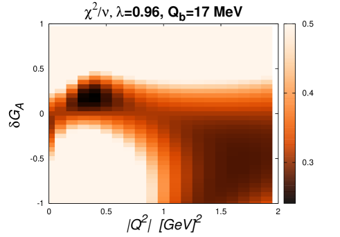
In order to study the sensibility of the results against general variations of the form factor, we also show in fig. 7 the $\chi^{2}/\nu$ contour plots for the errors in the axial form factor $\delta G_{A}(Q^{2})$ when the $Q^{2}$ values are binned with $\Delta Q^{2}=0.1\,{\rm GeV}^{2}$ in the range $Q^{2}\leq 2{\rm\,GeV}^{2}$. The $\chi^{2}$ for each value of $\delta G_{A}$ in a $Q^{2}$ bin has been computed by adding the specified value of $\delta G_{A}$ to the form factor at the $Q^{2}$ values of the corresponding bin only. This shows that the value of $\chi^{2}$ can be lowered further for more general variations of the axial form factor. To explore this issue deeper we have performed simultaneous variations of $\delta G_{A}(Q^{2})$ in twenty $Q^{2}$ bins. A new minimum was found giving $\chi^{2}=23.8$ and $\chi^{2}/\nu=0.17$. As seen in fig. 7 —and verified by our minimization— the data seems to favor a larger form factor around $Q^{2}=0.4$ GeV² and a smaller one around 1.2 – 2 GeV².

Figure 7: Top panel: $\chi^{2}$ contour plot for the fitted axial masses. Bottom panel: $\chi^{2}$ contour plots for the errors in the axial form factor $\delta G_{A}(Q^{2})$ when the $Q^{2}$ values are binned with $\Delta Q^{2}=0.1\,{\rm GeV}^{2}$ in the range $0.1\,{\rm GeV}^{2}\leq Q^{2}\leq 2\,{\rm GeV}^{2}$.

Note that, while our analysis here is focused on the quasielastic neutrino-nucleus scattering, similar meson-dominance ideas for the nucleon and $\Delta$-resonance have been discussed in previous work by Dominguez and collaborators Dominguez:2004bx ; Dominguez:2007hg suggesting a possible extension to $N-\Delta$ transition form factors.

VI Conclusions and outlook

Most of the previous analyzes of the axial form factor assuming a dipolar form and fitting MiniBoone neutrino-nucleus scattering data provide unprecedented accurate but incompatible determinations of the dipolar axial mass, regardless of the assumed nuclear model. This suggests that while the proposed dipolar parameterization minimizes the mean squared distance between theory and data, it does not account properly for the experimental data fluctuations, introducing a systematic bias and invalidating the conventional least squares fitting strategy assumptions. Besides, the large spread of the many experimental data for the axial form factor is not sharpened by the currently available lattice QCD calculations or QCD sum rules estimates, where a direct determination of the axial current matrix element has been undertaken. As a consequence, the validation of known nuclear effects in neutrino-nucleus scattering is hampered by the many contradicting determinations of the axial form factor already in the quasielastic region.

We take here a different perspective admitting from the beginning the existence of an uncertainty band in the axial form factor. We assume a theoretically based axial form factor with an a priori uncertainty estimate, regardless of the neutrino data we intend to describe. Namely, we use the minimal AVMD compatible with pQCD, an ansatz motivated by quite general large $N_{c}$ features and which requires just the $a_{1}$ and $a_{1}^{\prime}$ mesons to be saturated. As it has been done in previous determinations of other hadronic and generalized form factors we have taken as an educated guess the half width rule for the axial-vector isovector masses. The produced spread is fairly consistent with the current experimental and lattice spread of values.

Most remarkably the errors in the axial form factor determined by the axial-vector dominance and using the half width rule, while quite generous, do not generally produce larger uncertainties in the neutrino-nucleus scattering than the experimental differential cross sections reported by the MiniBoone collaboration. We have also provided evidence that the region of the axial form factor having most impact in the MiniBooNE data is in the range $0.2\lesssim Q^{2}\lesssim 0.6\,{\rm GeV}^{2}$, whereas fluctuations outside this regime tend to be marginal. We stress that these features cannot be captured by the conventional dipole parameterization.

Of course the minimal hadronic ansatz could be improved by adding other poles from the PDG axial mesons compilation. In the case of three poles, unlike the present case additional unknown information such as e.g. the coupling of the third meson to the nucleon is needed. One could expect that the future neutrino data might be accurate enough to pin down this extra parameter.

Our analysis has been carried out using the RFG model which for the quasielastic region does not seem to miss effects which are larger than the present uncertainty in the axial form factor using the AVMD ansatz supplemented with the half-width rule. The role of additional nuclear effects improving the present model will be presented in further work. The role played at higher energies by the equivalent AVMD form factors and further nuclear mechanisms remains to be seen.

References

- (1) A. Aguilar-Arevalo et al. (MiniBooNE Collaboration), Phys. Rev. Lett. 100, 032301 (2008).
- (2) A. Aguilar-Arevalo et al. (MiniBooNE Collaboration), Phys. Rev. D 81, 092005 (2010).
- (3) A. Aguilar-Arevalo et al. (MiniBooNE Collaboration), Phys. Rev. D 88, 032001 (2013).
- (4) H. Gallagher, G. Garvey, G.P. Zeller, Annu. Rev. Nucl. Part. Sci. 61, 355 (2011).
- (5) J.A. Formaggio, G.P. Zeller, Rev. Mod. Phys. 84, 1307 (2012).
- (6) J.G. Morfin, J. Nieves, J.T. Sobczyk, Adv. High Energy Phys. 2012, 934597 (2012).
- (7) L. Alvarez-Ruso, Y. Hayato, and J. Nieves, New Jou. Phys. 16 (2014) 075015.
- (8) J. Nieves, I. Ruiz Simo, M.J. Vicente Vacas, Phys. Lett. B 707 (2012) 72.
- (9) A.V. Butkevich, D. Perevalov, Phys. Rev. D 89 (2014) 053014.
- (10) A. Liesenfeld et al. [A1 Collaboration], Phys. Lett. B 468, 20 (1999).
- (11) V. Bernard, L. Elouadrhiri, and U.G. Meissner, Jou. Phys. G: Nucl. Part. Phys. 28 (2002) R1.
- (12) M. Martini, M. Ericson, G. Chanfray, J. Marteau, Phys. Rev. C 81 (2010) 045502.
- (13) J.E. Amaro, M.B. Barbaro, J.A. Caballero, T.W. Donnelly, C.F. Williamson, Phys. lett. B 696 (2011) 151.
- (14) G.D. Megias, J.E. Amaro, M.B. barbaro, J.A. Caballero, T.W. Donnelly, Phys. lett. B 725 (2013) 170.
- (15) J. E. Amaro, E. R. Arriola and I. R. Simo, Phys. Rev. C 92, 054607 (2015).
- (16) C. Wilkinson [T2K Collaboration], PoS NUFACT 2014, 104 (2015)
- (17) P. Masjuan, E. Ruiz-Arriola, W. Broniowski, Phys. Rev. D 87, 014005 (2013).
- (18) Carl E. Carlson and J. L. Poor. Phys. Rev., D34:1478, 1986.
- (19) Bhubanjyoti Bhattacharya, Richard J. Hill, and Gil Paz. Phys. Rev., D84:073006, 2011.
- (20) A. Bodek, S. Avvakumov, R. Bradford, and Howard Scott Budd. Eur. Phys. J., C53:349–354, 2008.
- (21) K. F. Liu, S. J. Dong, Terrence Draper, J. M. Wu, and W. Wilcox. Phys. Rev., D49:4755–4761, 1994.
- (22) S. Capitani et al. Nucl. Phys. Proc. Suppl., 73:294–296, 1999.
- (23) C. Alexandrou et al. Phys. Rev., D83:045010, 2011.
- (24) Parikshit M. Junnarkar, S. Capitani, D. Djukanovic, G. von Hippel, J. Hua, B. Jäger, H. B. Meyer, T. D. Rae, and H. Wittig. PoS, LATTICE2014:150, 2015.
- (25) V. M. Braun, A. Lenz, and M. Wittmann. Phys. Rev., D73:094019, 2006.
- (26) Zhi-Gang Wang, Shao-Long Wan, and Wei-Min Yang. Eur. Phys. J., C47:375–384, 2006.
- (27) Guray Erkol and Altug Ozpineci. Phys. Rev., D83:114022, 2011.
- (28) T. D. Lee, S. Weinberg, and B. Zumino. Phys. Rev. Lett., 18:1029–1032, 1967.
- (29) T. D. Lee and B. Zumino. Phys. Rev., 163:1667–1681, 1967.
- (30) P. H. Frampton. Phys. Rev., D1:3141–3151, 1970.
- (31) M. Gari and U. Kaulfuss. Phys. Lett., B138:29–31, 1984.
- (32) Gerard ’t Hooft. Nucl. Phys., B72:461, 1974.
- (33) Edward Witten. Nucl. Phys., B160:57, 1979.
- (34) P. Masjuan, E. Ruiz Arriola, and W. Broniowski. Phys. Rev., D85:094006, 2012.
- (35) C. A. Dominguez and O. Zandron, Nucl. Phys. B 33, 303 (1971).
- (36) C. A. Dominguez and O. Zandron, Nuovo Cim. A 3, 298 (1971).
- (37) C. A. Dominguez, Phys. Rev. D 15, 1350 (1977).
- (38) C. A. Dominguez, Phys. Rev. D 16, 2313 (1977).
- (39) C. A. Dominguez, Phys. Rev. D 16, 2320 (1977).
- (40) C. A. Dominguez, Riv. Nuovo Cim. 8N6, 1 (1985).
- (41) J. Beringer et al. Phys. Rev., D86:010001, 2012.
- (42) Y. Nambu and M. Yoshimura, Phys. Rev. lett. 24, 25 (1970).
- (43) G. Benfatto, F. Nicolo, and G.C. Rossi, Nuovo Cimento A 14, 425 (1973).
- (44) G. Furlan, N. Paver, and C. Verzegnassi, Nuovo Cimento A 70, 247 (1970).
- (45) N. Dombey and B.J. Read, Nucl. Phys. B 60, 65 (1973).
- (46) P. Joos et al., Phys. lett. B 62, 230 (1976).
- (47) N.J. Baker et al., Phys. Rev. D 23, 2499 (1981).
- (48) K.L. Miller et al., Phys. Rev. D 26, 537 (1982).
- (49) T. Kitagaki, et al., Phys. Rev. D 28, 436 (1983).
- (50) T. Kitagaki, et al., Phys. Rev. D 42, 1331 (1990).
- (51) J.E. Amaro, M.B. Barbaro, J.A. Caballero, T.W. Donnelly A. Molinari, and I. Sick, Phys. Rev. C 71, 015501 (2005)
- (52) J.E. Amaro, M.B. Barbaro, J.A. Caballero, T.W. Donnelly, C. Maieron, Phys. Rev. C 71, 065501 (2005)
- (53) J.E. Amaro, M. B. Barbaro, J. A. Caballero, and T. W. Donnelly. Phys. Rev. Lett., 98:242501, 2007.
- (54) C. A. Dominguez and T. Thapedi, JHEP 0410, 003 (2004)
- (55) C. A. Dominguez and R. Rontsch, JHEP 0710, 085 (2007).