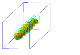
An adaptive finite element method in reconstruction of coefficients in Maxwell’s equations from limited observations

L. Beilina Department of Mathematical Sciences, Chalmers University of Technology and Gothenburg University, SE-42196 Gothenburg, Sweden, e-mail:  larisa@chalmers.se    S. Hosseinzadegan Department of Mathematical Sciences, Chalmers University of Technology and Gothenburg University, SE-42196 Gothenburg, Sweden,e-mail:  samarh@student.chalmers.se
Abstract

We propose an adaptive finite element method for the solution of a coefficient inverse problem of simultaneous reconstruction of the dielectric permittivity and magnetic permeability functions in the Maxwell’s system using limited boundary observations of the electric field in 3D.

We derive a posteriori error estimates in the Tikhonov functional to be minimized and in the regularized solution of this functional, as well as formulate corresponding adaptive algorithm. Our numerical experiments justify the efficiency of our a posteriori estimates and show significant improvement of the reconstructions obtained on locally adaptively refined meshes.

1 Introduction

This work is a continuation of the recent paper [7] and is focused on the numerical reconstruction of the dielectric permittivity ε(x)𝜀𝑥\varepsilon(x) and the magnetic permeability μ(x)𝜇𝑥\mu(x) functions in the Maxwell’s system on locally refined meshes using an adaptive finite element method. The reconstruction is performed via minimization of the corresponding Tikhonov functional from backscattered single measurement data of the electric field E(x,t)𝐸𝑥𝑡E(x,t). That means that we use backscattered boundary measurements of the wave field E(x,t)𝐸𝑥𝑡E(x,t) which are generated by a single direction of a plane wave. In the minimization procedure we use domain decomposition finite element/finite difference methods of [5] for the numerical reconstructions of both functions.

Comparing with [7] we present following new points here: we adopt results of [10, 11, 30] to show that the minimizer of the Tikhonov functional is closer to the exact solution than guess of this solution. We present relaxation property for the mesh refinements for the case of our inverse problem and we derive a posteriori error estimates for the error in the minimization functional and in the reconstructed functions ε(x)𝜀𝑥\varepsilon(x) and μ(x)𝜇𝑥\mu(x). Further, we formulate two adaptive algorithms and apply them in the reconstruction of small inclusions. Moreover, in our numerical simulations of this work we induce inhomogeneous initial conditions in the Maxwell’s system. Non-zero initial conditions involve uniqueness and stability results of reconstruction of both unknown functions ε(x)𝜀𝑥\varepsilon(x) and μ(x)𝜇𝑥\mu(x), see details in [7, 13].

Using our numerical simulations we can conclude that an adaptive finite element method can significantly improve reconstructions obtained on a coarse non-refined mesh in order to accurately obtain shapes, locations and values of functions ε(x)𝜀𝑥\varepsilon(x) and μ(x)𝜇𝑥\mu(x).

An outline of this paper is as follows: in Section 2 we present our mathematical model and in Section 3 we formulate forward and inverse problems. In Section 4 we present the Tikhonov functional to be minimized and in Section 5 we show different versions of finite element method used in computations. In Section 6 we formulate relaxation property of mesh refinements and in Section 7 we investigate general framework of a posteriori error estimates in coefficient inverse problems (CIPs). In Sections 8, 9 we present theorems for a posteriori errors in the regularized solution of the Tikhonov functional and in the Tikhonov functional, correspondingly. In Sections 10, 11 we describe mesh refinement recommendations and formulate adaptive algorithms used in computations. Finally, in Section 12 we present our reconstruction results.

2 The mathematical model

Let a bounded domain Ωd,d=2,3,formulae-sequenceΩsuperscript𝑑𝑑23\Omega\subset\mathbb{R}^{d},d=2,3, have Lipschitz boundary ΩΩ\partial\Omega and let us set ΩT:=Ω×(0,T)assignsubscriptΩ𝑇Ω0𝑇\Omega_{T}:=\Omega\times(0,T), ΩT:=Ω×(0,T)assignsubscriptΩ𝑇Ω0𝑇\partial\Omega_{T}:=\partial\Omega\times(0,T), where T>0𝑇0T>0. We consider Maxwell’s equations in an inhomogeneous isotropic media in a bounded domain Ω3Ωsuperscript3\Omega\subset\mathbb{R}^{3}

{tD×H(x,t)=0 in ΩTtB+×E(x,t)=0 in ΩT,D(x,t)=εE(x,t),B(x,t)=μH(x,t),E(x,0)=E0(x),H(x,0)=H0(x),D(x,t)=0,B(x,t)=0 in ΩT,n×D(x,t)=0,nB(x,t)=0on ΩT,casessubscript𝑡𝐷𝐻𝑥𝑡0missing-subexpression in subscriptΩ𝑇missing-subexpressionmissing-subexpressionmissing-subexpressionsubscript𝑡𝐵𝐸𝑥𝑡0missing-subexpression in subscriptΩ𝑇missing-subexpressionmissing-subexpressionmissing-subexpressionformulae-sequence𝐷𝑥𝑡𝜀𝐸𝑥𝑡𝐵𝑥𝑡𝜇𝐻𝑥𝑡missing-subexpressionmissing-subexpressionmissing-subexpressionmissing-subexpressionmissing-subexpressionformulae-sequence𝐸𝑥0subscript𝐸0𝑥𝐻𝑥0subscript𝐻0𝑥missing-subexpressionmissing-subexpressionmissing-subexpressionmissing-subexpressionmissing-subexpressionformulae-sequence𝐷𝑥𝑡0𝐵𝑥𝑡0missing-subexpression in subscriptΩ𝑇missing-subexpressionmissing-subexpressionmissing-subexpressionformulae-sequence𝑛𝐷𝑥𝑡0𝑛𝐵𝑥𝑡0missing-subexpressionon subscriptΩ𝑇missing-subexpressionmissing-subexpressionmissing-subexpression\left\{\begin{array}[]{llllll}\partial_{t}D-\nabla\times H(x,t)=0&&\mbox{ in }\Omega_{T}\\ \partial_{t}B+\nabla\times E(x,t)=0&&\mbox{ in }\Omega_{T},\\ D(x,t)=\varepsilon E(x,t),\quad B(x,t)=\mu H(x,t),&&\\ E(x,0)=E_{0}(x),\quad H(x,0)=H_{0}(x),&&\\ \nabla\cdot D(x,t)=0,\quad\nabla\cdot B(x,t)=0&&\mbox{ in }\Omega_{T},\\ n\times D(x,t)=0,\quad n\cdot B(x,t)=0&&\textrm{on }\,\partial\Omega_{T},\end{array}\right. (1)

where x=(x1,x2,x3)𝑥subscript𝑥1subscript𝑥2subscript𝑥3x=(x_{1},x_{2},x_{3}). Here, E(x,t)𝐸𝑥𝑡E(x,t) is the electric field and H(x,t)𝐻𝑥𝑡H(x,t) is the magnetic field, ε(x)>0𝜀𝑥0\varepsilon(x)>0 and μ(x)>0𝜇𝑥0\mu(x)>0 are the dielectric permittivity and the magnetic permeability functions, respectively. E0(x)subscript𝐸0𝑥E_{0}(x) and H0(x)subscript𝐻0𝑥H_{0}(x) are given initial conditions. Next, n=n(x)𝑛𝑛𝑥n=n(x) is the unit outward normal vector to ΩΩ\partial\Omega. The electric field E(x,t)𝐸𝑥𝑡E(x,t) is combined with the electric induction D(x,t)𝐷𝑥𝑡D(x,t) via

D(x,t)=εE(x,t)=εvacεrE(x,t),𝐷𝑥𝑡𝜀𝐸𝑥𝑡subscript𝜀vacsubscript𝜀𝑟𝐸𝑥𝑡D(x,t)=\varepsilon E(x,t)=\varepsilon_{\rm vac}\varepsilon_{r}E(x,t),

where εvac8.854×1012subscript𝜀vac8.854superscript1012\varepsilon_{\rm vac}\approx 8.854\times 10^{-12} is the vacuum permittivity which is measured in Farads per meter, and thus εrsubscript𝜀𝑟\varepsilon_{r} is the dimensionless relative permittivity. The magnetic field H(x,t)𝐻𝑥𝑡H(x,t) is combined with the magnetic induction B(x,t)𝐵𝑥𝑡B(x,t) via

B(x,t)=μH(x,t)=μvacμrH(x,t),𝐵𝑥𝑡𝜇𝐻𝑥𝑡subscript𝜇vacsubscript𝜇𝑟𝐻𝑥𝑡B(x,t)=\mu H(x,t)=\mu_{\rm vac}\mu_{r}H(x,t),

where μvac1.257×106subscript𝜇vac1.257superscript106\mu_{\rm vac}\approx 1.257\times 10^{-6} is the vacuum permeability measured in Henries per meter, from what follows that μrsubscript𝜇𝑟\mu_{r} is the dimensionless relative permeability.

By eliminating B𝐵B and D𝐷D from (1) we obtain the model problem for the electric field E𝐸E with the perfectly conducting boundary conditions which is as follows:

ε2Et2+×(μ1×E)𝜀superscript2𝐸superscript𝑡2superscript𝜇1𝐸\displaystyle\varepsilon\frac{\partial^{2}E}{\partial t^{2}}+\nabla\times(\mu^{-1}\nabla\times E) =\displaystyle= 0inΩT,0insubscriptΩ𝑇\displaystyle 0~{}\mbox{in}~{}~{}\Omega_{T}, (2)
(εE)𝜀𝐸\displaystyle\nabla\cdot(\varepsilon E) =\displaystyle= 0inΩT,0insubscriptΩ𝑇\displaystyle 0~{}\mbox{in}~{}~{}\Omega_{T}, (3)
E(x,0)=f0(x),Et(x,0)𝐸𝑥0subscript𝑓0𝑥subscript𝐸𝑡𝑥0\displaystyle E(x,0)=f_{0}(x),~{}~{}~{}E_{t}(x,0) =\displaystyle= f1(x)inΩ,subscript𝑓1𝑥inΩ\displaystyle f_{1}(x)~{}\mbox{in}~{}~{}\Omega, (4)
E×n𝐸𝑛\displaystyle E\times n =\displaystyle= 0onΩT.0onsubscriptΩ𝑇\displaystyle 0~{}\mbox{on}~{}~{}\partial\Omega_{T}. (5)

Here we assume that

f0H1(Ω),f1L2(Ω).formulae-sequencesubscript𝑓0superscript𝐻1Ωsubscript𝑓1superscript𝐿2Ωf_{0}\in H^{1}(\Omega),f_{1}\in L^{2}(\Omega).

By this notation we shall mean that every component of the vector functions f0subscript𝑓0f_{0} and f1subscript𝑓1f_{1} belongs to these spaces. Note that equations similar to (2)-(5) can be derived also for the magnetic field H𝐻H.

As in our recent work [7], for the discretization of the Maxwell’s equations we use a stabilized domain decomposition method of [6]. In our numerical simulations we assume that the relative permittivity εrsubscript𝜀𝑟\varepsilon_{r} and relative permeability μrsubscript𝜇𝑟\mu_{r} does not vary much which is the case of real applications, see recent experimental work [8] for similar observations. We do not impose smoothness assumptions on the coefficients ε(x),μ(x)𝜀𝑥𝜇𝑥\varepsilon(x),\mu(x) and we treat discontinuities in a similar way as in [18]. Thus, a discontinuous finite element method should be applied for the finite element discretization of these functions, see details in Section 5.

3 Statements of forward and inverse problems

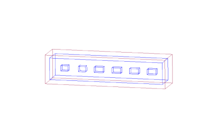
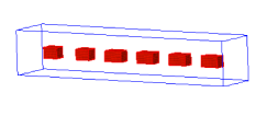
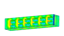
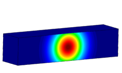
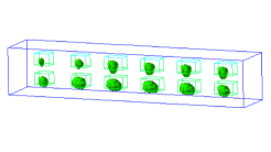
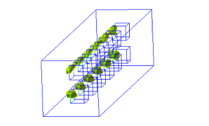
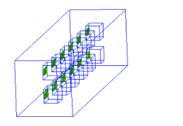
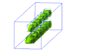
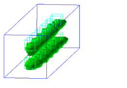
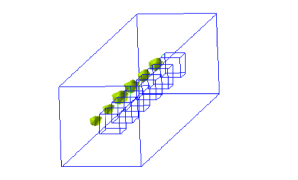
We divide ΩΩ\Omega into two subregions, ΩFEMsubscriptΩFEM\Omega_{\rm FEM} and ΩOUTsubscriptΩOUT\Omega_{\rm OUT} such that Ω¯=Ω¯FEMΩ¯OUT¯Ωsubscript¯ΩFEMsubscript¯ΩOUT\overline{\Omega}=\overline{\Omega}_{\rm FEM}\cup\overline{\Omega}_{\rm OUT}, ΩFEMΩOUT=subscriptΩFEMsubscriptΩOUT\Omega_{\rm FEM}\cap\Omega_{\rm OUT}=\emptyset and ΩFEMΩOUTsubscriptΩFEMsubscriptΩOUT\partial\Omega_{\rm FEM}\subset\partial\Omega_{\rm OUT}. For an illustration of the domain decomposition, see Figure 1. The boundary ΩΩ\partial\Omega is such that Ω=1Ω2Ω3ΩΩsubscript1Ωsubscript2Ωsubscript3Ω\partial\Omega=\partial_{1}\Omega\cup\partial_{2}\Omega\cup\partial_{3}\Omega where 1Ωsubscript1Ω\partial_{1}\Omega and 2Ωsubscript2Ω\partial_{2}\Omega are, respectively, front and back sides of the domain ΩΩ\Omega, and 3Ωsubscript3Ω\partial_{3}\Omega is the union of left, right, top and bottom faces of this domain. For numerical solution of (2)-(5) in ΩOUTsubscriptΩOUT\Omega_{\rm OUT} we can use either the finite difference or the finite element method on a structured mesh with constant coefficients ε=1𝜀1\varepsilon=1 and μ=1𝜇1\mu=1. In ΩFEMsubscriptΩFEM\Omega_{\rm FEM}, we use finite elements on a sequence of unstructured meshes Kh={K}subscript𝐾𝐾K_{h}=\{K\}, with elements K𝐾K consisting of triangles in 2superscript2\mathbb{R}^{2} and tetrahedra in 3superscript3\mathbb{R}^{3} satisfying the maximal angle condition [16].
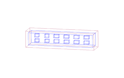
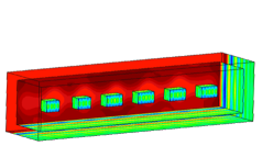
Refer to caption Refer to caption
a) Test1: Ω=ΩFEMΩOUTΩsubscriptΩ𝐹𝐸𝑀subscriptΩ𝑂𝑈𝑇\Omega=\Omega_{FEM}\cup\Omega_{OUT} b) Test 1: ΩFEMsubscriptΩ𝐹𝐸𝑀\Omega_{FEM}
Refer to caption Refer to caption
c) Test 2: Ω=ΩFEMΩOUTΩsubscriptΩ𝐹𝐸𝑀subscriptΩ𝑂𝑈𝑇\Omega=\Omega_{FEM}\cup\Omega_{OUT} d) Test 2: ΩFEMsubscriptΩ𝐹𝐸𝑀\Omega_{FEM}
Figure 1: Domain decomposition in numerical tests of Section 12. a), c) The decomposed domain Ω=ΩFEMΩOUTΩsubscriptΩ𝐹𝐸𝑀subscriptΩ𝑂𝑈𝑇\Omega=\Omega_{FEM}\cup\Omega_{OUT}. b), d) The finite element domain ΩFEMsubscriptΩ𝐹𝐸𝑀\Omega_{FEM}.

Let ST:=1Ω×(0,T)assignsubscript𝑆𝑇subscript1Ω0𝑇S_{T}:=\partial_{1}\Omega\times(0,T) where 1Ωsubscript1Ω\partial_{1}\Omega is the backscattering side of the domain ΩΩ\Omega with the time domain observations, and define by S1,1:=1Ω×(0,t1]assignsubscript𝑆11subscript1Ω0subscript𝑡1S_{1,1}:=\partial_{1}\Omega\times(0,t_{1}], S1,2:=1Ω×(t1,T)assignsubscript𝑆12subscript1Ωsubscript𝑡1𝑇S_{1,2}:=\partial_{1}\Omega\times(t_{1},T), S2:=2Ω×(0,T)assignsubscript𝑆2subscript2Ω0𝑇S_{2}:=\partial_{2}\Omega\times(0,T), S3:=3Ω×(0,T)assignsubscript𝑆3subscript3Ω0𝑇S_{3}:=\partial_{3}\Omega\times(0,T).

To simplify notations, further we will omit subscript r𝑟r in εrsubscript𝜀𝑟\varepsilon_{r} and μrsubscript𝜇𝑟\mu_{r}. We add a Coulomb-type gauge condition [2, 32] to (2)-(5) for stabilization of the finite element solution using the standard piecewise continuous functions with 0s10𝑠10\leq s\leq 1, and our model problem (2)-(5) which we use in computations rewrites as

ε2Et2+×(μ1×E)s((εE))=0inΩT,E(x,0)=f0(x),Et(x,0)=f1(x)inΩ,nE=(0,f(t),0)onS1,1,nE=tEonS1,2,nE=tEonS2,nE=0onS3,μ(x)=ε(x)=1 in ΩOUT.formulae-sequence𝜀superscript2𝐸superscript𝑡2superscript𝜇1𝐸𝑠𝜀𝐸0insubscriptΩ𝑇formulae-sequence𝐸𝑥0subscript𝑓0𝑥formulae-sequencesubscript𝐸𝑡𝑥0subscript𝑓1𝑥inΩformulae-sequencesubscript𝑛𝐸0𝑓𝑡0onsubscript𝑆11formulae-sequencesubscript𝑛𝐸subscript𝑡𝐸onsubscript𝑆12formulae-sequencesubscript𝑛𝐸subscript𝑡𝐸onsubscript𝑆2formulae-sequencesubscript𝑛𝐸0onsubscript𝑆3𝜇𝑥𝜀𝑥1 in subscriptΩOUT\begin{split}\varepsilon\frac{\partial^{2}E}{\partial t^{2}}+\nabla\times(\mu^{-1}\nabla\times E)-s\nabla(\nabla\cdot(\varepsilon E))&=0~{}\mbox{in}~{}~{}\Omega_{T},\\ E(x,0)=f_{0}(x),~{}~{}~{}E_{t}(x,0)&=f_{1}(x)~{}\mbox{in}~{}~{}\Omega,\\ \partial_{n}E&=(0,f\left(t\right),0)~{}\mbox{on}~{}S_{1,1},\\ \partial_{n}E&=-\partial_{t}E~{}\mbox{on}~{}S_{1,2},\\ \partial_{n}E&=-\partial_{t}E~{}\mbox{on}~{}S_{2},\\ \partial_{n}E&=0~{}\mbox{on}~{}S_{3},\\ \mu(x)=\varepsilon\left(x\right)&=1\text{ in }\Omega_{\rm OUT}.\end{split} (6)

In the recent works [5, 7, 8] was demonstrated numerically that the solution of the problem (6) approximates well the solution of the original Maxwell’s system for the case when 1μ(x)2,1ε(x)15formulae-sequence1𝜇𝑥21𝜀𝑥151\leq\mu(x)\leq 2,1\leq\varepsilon(x)\leq 15 and s=1𝑠1s=1.

We assume that our coefficients ε(x),μ(x)𝜀𝑥𝜇𝑥\varepsilon\left(x\right),\mu(x) of equation (6) are such that

ε(x)[1,d1],d1=const.>1,ε(x)=1 for xΩOUT,μ(x)[1,d2],d2=const.>1,μ(x)=1 for xΩOUT,ε(x),μ(x)C2(3).\begin{split}\varepsilon\left(x\right)&\in\left[1,d_{1}\right],~{}~{}d_{1}=const.>1,~{}\varepsilon(x)=1\text{ for }x\in\Omega_{\rm OUT},\\ \mu(x)&\in\left[1,d_{2}\right],~{}~{}d_{2}=const.>1,~{}\mu(x)=1\text{ for }x\in\Omega_{\rm OUT},\\ \varepsilon\left(x\right),\mu(x)&\in C^{2}\left(\mathbb{R}^{3}\right).\end{split} (7)

In our numerical tests the values of constants d1,d2subscript𝑑1subscript𝑑2d_{1},d_{2} in (7) are chosen from experimental set-up similarly with [8, 37] and we assume that we know them a priori.

This is in agreement with the availability of a priori information for an ill-posed problem [3, 22, 39]. Through the work we use following notations: for any vector function u3𝑢superscript3u\in\mathbb{R}^{3} when we write uHk(Ω),k=1,2formulae-sequence𝑢superscript𝐻𝑘Ω𝑘12u\in H^{k}(\Omega),k=1,2, we mean that every component of the vector function u𝑢u belongs to this space. We consider the following

Inverse Problem (IP) Assume that the functions ε(x)𝜀𝑥\varepsilon\left(x\right) and μ(x)𝜇𝑥\mu(x)  satisfy conditions (7) for the known d1,d2>1subscript𝑑1subscript𝑑21d_{1},d_{2}>1 and they are unknown in the domain Ω\ΩOUT\ΩsubscriptΩOUT\Omega\backslash\Omega_{\rm OUT}. Determine the functions ε(x),μ(x)𝜀𝑥𝜇𝑥\varepsilon\left(x\right),\mu(x) for xΩ\ΩOUT,𝑥\ΩsubscriptΩOUTx\in\Omega\backslash\Omega_{\rm OUT},  assuming that the following function E~(x,t)~𝐸𝑥𝑡\tilde{E}\left(x,t\right) is known

E(x,t)=E~(x,t)(x,t)ST.𝐸𝑥𝑡~𝐸𝑥𝑡for-all𝑥𝑡subscript𝑆𝑇E\left(x,t\right)=\tilde{E}\left(x,t\right)~{}\forall\left(x,t\right)\in S_{T}. (8)

The function E~(x,t)~𝐸𝑥𝑡\tilde{E}\left(x,t\right) in (8) represents the time-dependent measurements of the electric wave field E(x,t)𝐸𝑥𝑡E(x,t) at the backscattering boundary 1Ωsubscript1Ω\partial_{1}\Omega. In real-life experiments, measurements are performed on a number of detectors, see details in our recent experimental work [8].

4 Tikhonov functional

We reformulate our inverse problem as an optimization problem, where we seek for two functions, the permittivity ε(x)𝜀𝑥\varepsilon(x) and permeability μ(x)𝜇𝑥\mu(x), which result in a solution of equations (6) with best fit to time and space domain observations E~~𝐸\tilde{E}, measured at a finite number of observation points on 1Ωsubscript1Ω\partial_{1}\Omega. Our goal is to minimize the Tikhonov functional

J(ε,μ):=J(E,ε,μ)=12ST(EE~)2zδ(t)𝑑σ𝑑t+12γ1Ω(εε0)2𝑑x+12γ2Ω(μμ0)2𝑑x,assign𝐽𝜀𝜇𝐽𝐸𝜀𝜇12subscriptsubscript𝑆𝑇superscript𝐸~𝐸2subscript𝑧𝛿𝑡differential-d𝜎differential-d𝑡12subscript𝛾1subscriptΩsuperscript𝜀subscript𝜀02differential-d𝑥12subscript𝛾2subscriptΩsuperscript𝜇subscript𝜇02differential-d𝑥\begin{split}J(\varepsilon,\mu):=J(E,\varepsilon,\mu)&=\frac{1}{2}\int_{S_{T}}(E-\tilde{E})^{2}z_{\delta}(t)d\sigma dt\\ &+\frac{1}{2}\gamma_{1}\int_{\Omega}(\varepsilon-\varepsilon_{0})^{2}~{}~{}dx+\frac{1}{2}\gamma_{2}\int_{\Omega}(\mu-\mu_{0})^{2}~{}~{}dx,\end{split} (9)

where E~~𝐸\tilde{E} is the observed electric field, E𝐸E satisfies the equations (6) and thus depends on ε𝜀\varepsilon and μ𝜇\mu, ε0subscript𝜀0\varepsilon_{0} is the initial guess for ε𝜀\varepsilon and μ0subscript𝜇0\mu_{0} is the initial guess for μ𝜇\mu, and γi,i=1,2formulae-sequencesubscript𝛾𝑖𝑖12\gamma_{i},i=1,2 are the regularization parameters. Here, zδ(t)subscript𝑧𝛿𝑡z_{\delta}(t) is a cut-off function, which is introduced to ensure that the compatibility conditions at Ω¯T{t=T}subscript¯Ω𝑇𝑡𝑇\overline{\Omega}_{T}\cap\left\{t=T\right\} for the adjoint problem (18) are satisfied, and δ>0𝛿0\delta>0 is a small number. The function zδsubscript𝑧𝛿z_{\delta} can be chosen as in [7].

Next, we introduce the following spaces of real valued vector functions

HE1:={wH1(ΩT):w(,0)=0},Hλ1:={wH1(ΩT):w(,T)=0},U1=HE1(ΩT)×Hλ1(ΩT)×C(Ω¯)×C(Ω¯),U0=L2(ΩT)×L2(ΩT)×L2(Ω)×L2(Ω).formulae-sequenceassignsuperscriptsubscript𝐻𝐸1conditional-set𝑤superscript𝐻1subscriptΩ𝑇𝑤00formulae-sequenceassignsuperscriptsubscript𝐻𝜆1conditional-set𝑤superscript𝐻1subscriptΩ𝑇𝑤𝑇0formulae-sequencesuperscript𝑈1superscriptsubscript𝐻𝐸1subscriptΩ𝑇superscriptsubscript𝐻𝜆1subscriptΩ𝑇𝐶¯Ω𝐶¯Ωsuperscript𝑈0subscript𝐿2subscriptΩ𝑇subscript𝐿2subscriptΩ𝑇subscript𝐿2Ωsubscript𝐿2Ω\begin{split}H_{E}^{1}&:=\{w\in H^{1}(\Omega_{T}):w(\cdot,0)=0\},\\ H_{\lambda}^{1}&:=\{w\in H^{1}(\Omega_{T}):w(\cdot,T)=0\},\\ U^{1}&=H_{E}^{1}(\Omega_{T})\times H_{\lambda}^{1}(\Omega_{T})\times C\left(\overline{\Omega}\right)\times C\left(\overline{\Omega}\right),\\ U^{0}&=L_{2}\left(\Omega_{T}\right)\times L_{2}\left(\Omega_{T}\right)\times L_{2}\left(\Omega\right)\times L_{2}\left(\Omega\right).\end{split} (10)

We also define the L2subscript𝐿2L_{2} inner product and the norm over ΩTsubscriptΩ𝑇\Omega_{T} and ΩΩ\Omega as

((u,v))ΩT=Ω0Tuv𝑑x𝑑t,u2=((u,u))ΩT,(u,v)Ω=Ωuv𝑑x,|u|2=(u,u)Ω.formulae-sequencesubscript𝑢𝑣subscriptΩ𝑇subscriptΩsuperscriptsubscript0𝑇𝑢𝑣differential-d𝑥differential-d𝑡formulae-sequencesuperscriptnorm𝑢2subscript𝑢𝑢subscriptΩ𝑇formulae-sequencesubscript𝑢𝑣ΩsubscriptΩ𝑢𝑣differential-d𝑥superscript𝑢2subscript𝑢𝑢Ω\begin{split}((u,v))_{\Omega_{T}}&=\int_{\Omega}\int_{0}^{T}uvdxdt,\\ ||u||^{2}&=((u,u))_{\Omega_{T}},\\ (u,v)_{\Omega}&=\int_{\Omega}uvdx,\\ |u|^{2}&=(u,u)_{\Omega}.\end{split}

To solve the minimization problem we take into account (7) and introduce the Lagrangian

L(u)=J(E,ε,μ)((εtλ,tE))ΩT(ελ(x,0),f1(x))Ω+((μ1×E,×λ))ΩT+s(((εE),λ))ΩT((λ,p(t)))S1,1+((λtE))S1,2+((λtE))S2,𝐿𝑢𝐽𝐸𝜀𝜇subscript𝜀subscript𝑡𝜆subscript𝑡𝐸subscriptΩ𝑇subscript𝜀𝜆𝑥0subscript𝑓1𝑥Ωsubscriptsuperscript𝜇1𝐸𝜆subscriptΩ𝑇𝑠subscript𝜀𝐸𝜆subscriptΩ𝑇subscript𝜆𝑝𝑡subscript𝑆11subscript𝜆subscript𝑡𝐸subscript𝑆12subscript𝜆subscript𝑡𝐸subscript𝑆2\begin{split}L(u)&=J(E,\varepsilon,\mu)-\left(\left(\varepsilon\partial_{t}\lambda,\partial_{t}E\right)\right)_{\Omega_{T}}-(\varepsilon\lambda(x,0),f_{1}(x))_{\Omega}+\left(\left(\mu^{-1}\nabla\times E,\nabla\times\lambda\right)\right)_{\Omega_{T}}\\ &+s\left(\left(\nabla\cdot(\varepsilon E),\nabla\cdot\lambda\right)\right)_{\Omega_{T}}-((\lambda,p(t)))_{S_{1,1}}+((\lambda\partial_{t}E))_{S_{1,2}}+((\lambda\partial_{t}E))_{S_{2}},\\ \end{split} (11)

where u=(E,λ,ε,μ)U1𝑢𝐸𝜆𝜀𝜇superscript𝑈1u=(E,\lambda,\varepsilon,\mu)\in U^{1} and p(t)=(0,f(t),0)𝑝𝑡0𝑓𝑡0p(t)=(0,f(t),0) and tsubscript𝑡\partial_{t} define the derivative in time. We now search for a stationary point of the Lagrangian with respect to u𝑢u satisfying for all u¯=(E¯,λ¯,ε¯,μ¯)U1¯𝑢¯𝐸¯𝜆¯𝜀¯𝜇superscript𝑈1\bar{u}=(\bar{E},\bar{\lambda},\bar{\varepsilon},\bar{\mu})\in U^{1}

L(u;u¯)=0,superscript𝐿𝑢¯𝑢0L^{\prime}(u;\bar{u})=0, (12)

where L(u;)superscript𝐿𝑢L^{\prime}(u;\cdot) is the Jacobian of L𝐿L at u𝑢u. Equation above can be written as

L(u;u¯)=Lλ(u)(λ¯)+LE(u)(E¯)+Lε(u)(ε¯)+Lμ(u)(μ¯)=0.superscript𝐿𝑢¯𝑢𝐿𝜆𝑢¯𝜆𝐿𝐸𝑢¯𝐸𝐿𝜀𝑢¯𝜀𝐿𝜇𝑢¯𝜇0L^{\prime}(u;\bar{u})=\frac{\partial L}{\partial\lambda}(u)(\bar{\lambda})+\frac{\partial L}{\partial E}(u)(\bar{E})+\frac{\partial L}{\partial\varepsilon}(u)(\bar{\varepsilon})+\frac{\partial L}{\partial\mu}(u)(\bar{\mu})=0. (13)

To find the Frechét derivative (13) of the Lagrangian (11) we consider L(u+u¯)L(u)𝐿𝑢¯𝑢𝐿𝑢L(u+\bar{u})-L(u) for all u¯U1¯𝑢superscript𝑈1\bar{u}\in U^{1} and single out the linear part of the obtained expression with respect to u¯¯𝑢\bar{u}. In our derivation of the Frechét derivative we assume that in the Lagrangian (11) functions u=(E,λ,ε,μ)U1𝑢𝐸𝜆𝜀𝜇superscript𝑈1u=(E,\lambda,\varepsilon,\mu)\in U^{1} can vary independently of each other. In this approach we obtain the same result as by assuming that functions E𝐸E and λ𝜆\lambda are dependent on the coefficients ε,μ𝜀𝜇\varepsilon,\mu, see also Chapter 4 of [10] where similar observations take place. Taking into account that E(x,t)𝐸𝑥𝑡E(x,t) is the solution of the forward problem (6), assumptions that λ(x,T)=λt(x,T)=0𝜆𝑥𝑇𝜆𝑡𝑥𝑇0\lambda(x,T)=\frac{\partial\lambda}{\partial t}(x,T)=0, as well as μ=ε=1𝜇𝜀1\mu=\varepsilon=1 on ΩΩ\partial\Omega and using conditions (7), we obtain from (13) that for all u¯¯𝑢\bar{u},

0=Lλ(u)(λ¯)=((εtλ¯,tE))ΩT(εf1(x),λ¯(x,0))Ω+((μ1×E,×λ¯))ΩT+s(((εE),λ¯))ΩT((λ¯,p(t)))S1,1+((λ¯,tE))S1,2+((λ¯,tE))S2λ¯Hλ1(ΩT),0𝐿𝜆𝑢¯𝜆subscript𝜀subscript𝑡¯𝜆subscript𝑡𝐸subscriptΩ𝑇subscript𝜀subscript𝑓1𝑥¯𝜆𝑥0Ωsubscriptsuperscript𝜇1𝐸¯𝜆subscriptΩ𝑇𝑠subscript𝜀𝐸¯𝜆subscriptΩ𝑇subscript¯𝜆𝑝𝑡subscript𝑆11subscript¯𝜆subscript𝑡𝐸subscript𝑆12subscript¯𝜆subscript𝑡𝐸subscript𝑆2for-all¯𝜆superscriptsubscript𝐻𝜆1subscriptΩ𝑇\begin{split}0=\frac{\partial L}{\partial\lambda}(u)(\bar{\lambda})=&-((\varepsilon\partial_{t}\bar{\lambda},\partial_{t}E))_{\Omega_{T}}-(\varepsilon f_{1}(x),\bar{\lambda}(x,0))_{\Omega}+((\mu^{-1}\nabla\times E,\nabla\times\bar{\lambda}))_{\Omega_{T}}\\ &+s((\nabla\cdot(\varepsilon E),\nabla\cdot\bar{\lambda}))_{\Omega_{T}}-((\bar{\lambda},p(t)))_{S_{1,1}}+((\bar{\lambda},\partial_{t}E))_{S_{1,2}}\\ &+((\bar{\lambda},\partial_{t}E))_{S_{2}}~{}~{}\forall\bar{\lambda}\in H_{\lambda}^{1}(\Omega_{T}),\end{split} (14)
0=LE(u)(E¯)=((EE~,E¯zδ))ST((εtλ,tE¯))ΩT+((μ1×λ,×E¯))ΩT+s((λ,(εE¯))ΩT((tλ,E¯))S1,2S2(εE¯(x,0),tλ(x,0))E¯HE1(ΩT).\begin{split}0=\frac{\partial L}{\partial E}(u)(\bar{E})&=((E-\tilde{E},\bar{E}z_{\delta}))_{S_{T}}-((\varepsilon\partial_{t}\lambda,\partial_{t}\bar{E}))_{\Omega_{T}}+((\mu^{-1}\nabla\times\lambda,\nabla\times\bar{E}))_{\Omega_{T}}\\ &+s((\nabla\cdot\lambda,\nabla\cdot(\varepsilon\bar{E}))_{\Omega_{T}}-((\partial_{t}\lambda,\bar{E}))_{S_{1,2}\cup S_{2}}-(\varepsilon\bar{E}(x,0),\partial_{t}\lambda(x,0))~{}~{}\forall\bar{E}\in H_{E}^{1}(\Omega_{T}).\end{split} (15)

Further, we obtain two equations that express that the gradients with respect to ε𝜀\varepsilon and μ𝜇\mu vanish:

0=Lε(u)(ε¯)=((tλ,tEε¯))ΩT(λ(x,0),f1(x)ε¯)Ω+s(((ε¯E),λ))ΩT+γ1(εε0,ε¯)ΩxΩ,0𝐿𝜀𝑢¯𝜀subscriptsubscript𝑡𝜆subscript𝑡𝐸¯𝜀subscriptΩ𝑇subscript𝜆𝑥0subscript𝑓1𝑥¯𝜀Ω𝑠subscript¯𝜀𝐸𝜆subscriptΩ𝑇subscript𝛾1subscript𝜀subscript𝜀0¯𝜀Ωfor-all𝑥Ω\begin{split}0=\frac{\partial L}{\partial\varepsilon}(u)(\bar{\varepsilon})=&-((\partial_{t}\lambda,\partial_{t}E~{}\bar{\varepsilon}))_{\Omega_{T}}-(\lambda(x,0),f_{1}(x)~{}\bar{\varepsilon})_{\Omega}\\ &+s((\nabla\cdot(\bar{\varepsilon}E),\nabla\cdot\lambda))_{\Omega_{T}}+\gamma_{1}(\varepsilon-\varepsilon_{0},\bar{\varepsilon})_{\Omega}~{}~{}\forall x\in\Omega,\end{split} (16)
0=Lμ(u)(μ¯)=((μ2×E,×λμ¯))ΩT+γ2(μμ0,μ¯)ΩxΩ.0𝐿𝜇𝑢¯𝜇subscriptsuperscript𝜇2𝐸𝜆¯𝜇subscriptΩ𝑇subscript𝛾2subscript𝜇subscript𝜇0¯𝜇Ωfor-all𝑥Ω0=\frac{\partial L}{\partial\mu}(u)(\bar{\mu})=-((\mu^{-2}~{}\nabla\times E,\nabla\times\lambda~{}\bar{\mu}))_{\Omega_{T}}+\gamma_{2}(\mu-\mu_{0},\bar{\mu})_{\Omega}~{}\forall x\in\Omega. (17)

We observe that the equation (14) is the weak formulation of the state equation (6) and the equation (15) is the weak formulation of the following adjoint problem

ε2λt2+×(μ1×λ)sε(λ)=(EE~)|STzδ in ΩT,λ(,T)=λt(,T)=0,nλ=tλonS1,2,nλ=tλonS2,nλ=0onS3,formulae-sequenceformulae-sequence𝜀superscript2𝜆superscript𝑡2superscript𝜇1𝜆𝑠𝜀𝜆evaluated-at𝐸~𝐸subscript𝑆𝑇subscript𝑧𝛿 in subscriptΩ𝑇𝜆𝑇𝜆𝑡𝑇0formulae-sequencesubscript𝑛𝜆subscript𝑡𝜆onsubscript𝑆12formulae-sequencesubscript𝑛𝜆subscript𝑡𝜆onsubscript𝑆2subscript𝑛𝜆0onsubscript𝑆3\begin{split}\varepsilon\frac{\partial^{2}\lambda}{\partial t^{2}}+\nabla\times(\mu^{-1}\nabla\times\lambda)-s\varepsilon\nabla(\nabla\cdot\lambda)&=-(E-\tilde{E})|_{S_{T}}z_{\delta}~{}\mbox{ in }\Omega_{T},\\ \lambda(\cdot,T)&=\frac{\partial\lambda}{\partial t}(\cdot,T)=0,\\ \partial_{n}\lambda&=\partial_{t}\lambda~{}\mbox{on}~{}S_{1,2},\\ \partial_{n}\lambda&=\partial_{t}\lambda~{}\mbox{on}~{}S_{2},\\ \partial_{n}\lambda&=0~{}\mbox{on}~{}S_{3},\end{split} (18)

which is solved backward in time.

We now define by E(ε,μ),λ(ε,μ)𝐸𝜀𝜇𝜆𝜀𝜇E(\varepsilon,\mu),\lambda(\varepsilon,\mu) the exact solutions of the forward and adjoint problems for given ε,μ𝜀𝜇\varepsilon,\mu, respectively. Then defining by

u(ε,μ)=(E(ε,μ),λ(ε,μ),ε,μ)U1,𝑢𝜀𝜇𝐸𝜀𝜇𝜆𝜀𝜇𝜀𝜇superscript𝑈1u(\varepsilon,\mu)=(E(\varepsilon,\mu),\lambda(\varepsilon,\mu),\varepsilon,\mu)\in U^{1},

using the fact that for exact solutions E(ε,μ),λ(ε,μ)𝐸𝜀𝜇𝜆𝜀𝜇E(\varepsilon,\mu),\lambda(\varepsilon,\mu) because of (11) we have

J(E(ε,μ),ε,μ)=L(u(ε,μ)),𝐽𝐸𝜀𝜇𝜀𝜇𝐿𝑢𝜀𝜇J(E(\varepsilon,\mu),\varepsilon,\mu)=L(u(\varepsilon,\mu)), (19)

and assuming that solutions E(ε,μ),λ(ε,μ)𝐸𝜀𝜇𝜆𝜀𝜇E(\varepsilon,\mu),\lambda(\varepsilon,\mu) are sufficiently stable, see Chapter 5 of book [31] for details, we can write that the Frechét derivative of the Tikhonov functional is the function J(ε,μ,E(ε,μ))superscript𝐽𝜀𝜇𝐸𝜀𝜇J^{\prime}(\varepsilon,\mu,E(\varepsilon,\mu)) which is defined as

J(ε,μ):=J(ε,μ,E(ε,μ))=Jε(ε,μ,E(ε,μ))+Jμ(ε,μ,E(ε,μ))=Lε(u(ε,μ))+Lμ(u(ε,μ)).assignsuperscript𝐽𝜀𝜇superscript𝐽𝜀𝜇𝐸𝜀𝜇𝐽𝜀𝜀𝜇𝐸𝜀𝜇𝐽𝜇𝜀𝜇𝐸𝜀𝜇𝐿𝜀𝑢𝜀𝜇𝐿𝜇𝑢𝜀𝜇\begin{split}J^{\prime}(\varepsilon,\mu):=J^{\prime}(\varepsilon,\mu,E(\varepsilon,\mu))&=\frac{\partial J}{\partial\varepsilon}(\varepsilon,\mu,E(\varepsilon,\mu))+\frac{\partial J}{\partial\mu}(\varepsilon,\mu,E(\varepsilon,\mu))\\ &=\frac{\partial L}{\partial\varepsilon}(u(\varepsilon,\mu))+\frac{\partial L}{\partial\mu}(u(\varepsilon,\mu)).\end{split} (20)

Inserting (16) and (17) into (20), we get

J(ε,μ)(x):=J(ε,μ,E(ε,μ))(x)=0TtλtE(x,t)dtλ(x,0)f1(x)+s0T(E)(λ)(x,t)𝑑t+γ1(εε0)(x)0T(μ2×E)(×λ)(x,t)𝑑t+γ2(μμ0)(x).assignsuperscript𝐽𝜀𝜇𝑥superscript𝐽𝜀𝜇𝐸𝜀𝜇𝑥superscriptsubscript0𝑇subscript𝑡𝜆subscript𝑡𝐸𝑥𝑡𝑑𝑡𝜆𝑥0subscript𝑓1𝑥𝑠superscriptsubscript0𝑇𝐸𝜆𝑥𝑡differential-d𝑡subscript𝛾1𝜀subscript𝜀0𝑥superscriptsubscript0𝑇superscript𝜇2𝐸𝜆𝑥𝑡differential-d𝑡subscript𝛾2𝜇subscript𝜇0𝑥\begin{split}J^{\prime}(\varepsilon,\mu)(x)&:=J^{\prime}(\varepsilon,\mu,E(\varepsilon,\mu))(x)=-\int_{0}^{T}\partial_{t}\lambda~{}\partial_{t}E~{}(x,t)~{}dt-\lambda(x,0)f_{1}(x)\\ &+s\int_{0}^{T}(\nabla\cdot E)(\nabla\cdot\lambda)~{}(x,t)~{}dt+\gamma_{1}(\varepsilon-\varepsilon_{0})(x)\\ &-\int_{0}^{T}(\mu^{-2}~{}\nabla\times E)(\nabla\times\lambda)~{}(x,t)~{}dt+\gamma_{2}(\mu-\mu_{0})(x).\end{split} (21)

5 Finite element method

5.1 Finite element spaces

For computations we discretize ΩFEM×(0,T)subscriptΩFEM0𝑇\Omega_{\rm FEM}\times(0,T) in space and time. For discretization in space we denote by Kh={K}subscript𝐾𝐾K_{h}=\{K\} a partition of the domain ΩFEMsubscriptΩFEM\Omega_{\rm FEM} into tetrahedra K𝐾K in 3superscript3\mathbb{R}^{3} or triangles in 2superscript2\mathbb{R}^{2}. We discretize the time interval (0,T)0𝑇(0,T) into subintervals J=(tk1,tk]𝐽subscript𝑡𝑘1subscript𝑡𝑘J=(t_{k-1},t_{k}] of uniform length τ=tktk1𝜏subscript𝑡𝑘subscript𝑡𝑘1\tau=t_{k}-t_{k-1} and denote the time partition by Jτ={J}subscript𝐽𝜏𝐽J_{\tau}=\{J\}. In our finite element space mesh Khsubscript𝐾K_{h} the elements K𝐾K are such that

Kh=KKhK=K1K2Kl,subscript𝐾subscript𝐾subscript𝐾𝐾subscript𝐾1subscript𝐾2subscript𝐾𝑙K_{h}=\cup_{K\in K_{h}}K=K_{1}\cup K_{2}...\cup K_{l},

where l𝑙l is the total number of elements K𝐾K in Ω¯¯Ω\overline{\Omega}.

Similarly with [26] we introduce the mesh function h=h(x)𝑥h=h(x) which is a piecewise-constant function such that

h|K=hKKKh,evaluated-at𝐾subscript𝐾for-all𝐾subscript𝐾h|_{K}=h_{K}~{}~{}~{}\forall K\in K_{h}, (22)

where hKsubscript𝐾h_{K} is the diameter of K𝐾K which we define as the longest side of K𝐾K. Let rsuperscript𝑟r^{\prime} be the radius of the maximal circle/sphere contained in the element K𝐾K. For every element KKh𝐾subscript𝐾K\in K_{h} we assume the following shape regularity assumption

a1hKra2;a1,a2=const.>0.a_{1}\leq h_{K}\leq r^{\prime}a_{2};\quad a_{1},a_{2}=const.>0. (23)

To formulate the finite element method for (13), we define the finite element spaces. First we introduce the finite element trial space WhEsuperscriptsubscript𝑊𝐸W_{h}^{E} for every component of the electric field E𝐸E defined by

WhE:={wHE1:w|K×JP1(K)×P1(J),KKh,JJτ},assignsuperscriptsubscript𝑊𝐸conditional-set𝑤superscriptsubscript𝐻𝐸1formulae-sequenceevaluated-at𝑤𝐾𝐽subscript𝑃1𝐾subscript𝑃1𝐽formulae-sequencefor-all𝐾subscript𝐾for-all𝐽subscript𝐽𝜏W_{h}^{E}:=\{w\in H_{E}^{1}:w|_{K\times J}\in P_{1}(K)\times P_{1}(J),\forall K\in K_{h},\forall J\in J_{\tau}\},

where P1(K)subscript𝑃1𝐾P_{1}(K) and P1(J)subscript𝑃1𝐽P_{1}(J) denote the set of linear functions on K𝐾K and J𝐽J, respectively. We also introduce the finite element test space Whλsuperscriptsubscript𝑊𝜆W_{h}^{\lambda} defined by

Whλ:={wHλ1:w|K×JP1(K)×P1(J),KKh,JJτ}.assignsuperscriptsubscript𝑊𝜆conditional-set𝑤superscriptsubscript𝐻𝜆1formulae-sequenceevaluated-at𝑤𝐾𝐽subscript𝑃1𝐾subscript𝑃1𝐽formulae-sequencefor-all𝐾subscript𝐾for-all𝐽subscript𝐽𝜏W_{h}^{\lambda}:=\{w\in H_{\lambda}^{1}:w|_{K\times J}\in P_{1}(K)\times P_{1}(J),\forall K\in K_{h},\forall J\in J_{\tau}\}.

To approximate the functions μ(x)𝜇𝑥\mu(x) and ε(x)𝜀𝑥\varepsilon(x) we will use the space of piecewise constant functions VhL2(Ω)subscript𝑉subscript𝐿2ΩV_{h}\subset L_{2}(\Omega),

Vh:={uL2(Ω):u|KP0(K),KKh},assignsubscript𝑉conditional-set𝑢subscript𝐿2Ωformulae-sequenceevaluated-at𝑢𝐾subscript𝑃0𝐾for-all𝐾subscript𝐾V_{h}:=\{u\in L_{2}(\Omega):u|_{K}\in P_{0}(K),\forall K\in K_{h}\},

where P0(K)subscript𝑃0𝐾P_{0}(K) is the space of piecewise constant functions on K𝐾K. In some numerical experiments we will use also the space of piecewise linear functions WhH1(Ω)subscript𝑊superscript𝐻1ΩW_{h}\subset H^{1}(\Omega),

Wh={v(x)H1(Ω):v|KP1(K)KKh}.subscript𝑊conditional-set𝑣𝑥superscript𝐻1Ωevaluated-at𝑣𝐾subscript𝑃1𝐾for-all𝐾subscript𝐾W_{h}=\big{\{}v(x)\in H^{1}(\Omega):~{}v|_{K}\in P_{1}(K)~{}\forall K\in K_{h}\big{\}}. (24)

In a general case we allow the functions ε(x),μ(x)𝜀𝑥𝜇𝑥\varepsilon(x),\mu(x) to be discontinuous, see [KN]. Let Fhsubscript𝐹F_{h} be the set of all faces of elements in Khsubscript𝐾K_{h} such that Fh:=FhIFhBassignsubscript𝐹superscriptsubscript𝐹𝐼superscriptsubscript𝐹𝐵F_{h}:=F_{h}^{I}\cup F_{h}^{B}, where FhIsuperscriptsubscript𝐹𝐼F_{h}^{I} is the set of all interior faces and FhBsuperscriptsubscript𝐹𝐵F_{h}^{B} is the set of all boundary faces of elements in Khsubscript𝐾K_{h}. Let fFhI𝑓superscriptsubscript𝐹𝐼f\in F_{h}^{I} be the internal face of the non-empty intersection of the boundaries of two neighboring elements K+superscript𝐾K^{+} and Ksuperscript𝐾K^{-}. We denote the jump of the function vhsubscript𝑣v_{h} computed from the two neighboring elements K+superscript𝐾K^{+} and Ksuperscript𝐾K^{-} sharing the common side f𝑓f as

[vh]=vh+vh,delimited-[]subscript𝑣superscriptsubscript𝑣superscriptsubscript𝑣[v_{h}]=v_{h}^{+}-v_{h}^{-}, (25)

and the jump of the normal component vhsubscript𝑣v_{h} across the side f𝑓f as

[[vh]]=vh+n++vhn,delimited-[]delimited-[]subscript𝑣superscriptsubscript𝑣superscript𝑛superscriptsubscript𝑣superscript𝑛[[v_{h}]]=v_{h}^{+}\cdot n^{+}+v_{h}^{-}\cdot n^{-}, (26)

where n+,nsuperscript𝑛superscript𝑛n^{+},n^{-} is the unit outward normal on f+,fsuperscript𝑓superscript𝑓f^{+},f^{-}, respectively.

Let Phsubscript𝑃P_{h} be the L2(Ω)subscript𝐿2ΩL_{2}(\Omega) orthogonal projection. We define by fhIsuperscriptsubscript𝑓𝐼f_{h}^{I} the standard nodal interpolant [26] of f𝑓f into the space of continuous piecewise-linear functions on the mesh Khsubscript𝐾K_{h}. Then by one of properties of the orthogonal projection

fPhfL2(Ω)ffhIL2(Ω).subscriptnorm𝑓subscript𝑃𝑓subscript𝐿2Ωsubscriptnorm𝑓superscriptsubscript𝑓𝐼subscript𝐿2Ω\left\|f-P_{h}f\right\|_{L_{2}\left(\Omega\right)}\leq\left\|f-f_{h}^{I}\right\|_{L_{2}\left(\Omega\right)}. (27)

It follows from [36] that

fPhfL2(Ω)CIhfH1(Ω)fH1(Ω).subscriptnorm𝑓subscript𝑃𝑓subscript𝐿2Ωsubscript𝐶𝐼subscriptnorm𝑓superscript𝐻1Ωfor-all𝑓superscript𝐻1Ω\left\|f-P_{h}f\right\|_{L_{2}\left(\Omega\right)}\leq C_{I}h\left\|~{}f\right\|_{H^{1}\left(\Omega\right)}~{}~{}\forall f\in H^{1}(\Omega). (28)

where CI=CI(Ω)subscript𝐶𝐼subscript𝐶𝐼ΩC_{I}=C_{I}\left(\Omega\right) is a positive constant depending only on the domain ΩΩ\Omega.

5.2 A finite element method for optimization problem

To formulate the finite element method for (13) we define the space Uh=WhE×Whλ×Vh×Vhsubscript𝑈superscriptsubscript𝑊𝐸superscriptsubscript𝑊𝜆subscript𝑉subscript𝑉U_{h}=W_{h}^{E}\times W_{h}^{\lambda}\times V_{h}\times V_{h}. The finite element method reads: Find uhUhsubscript𝑢subscript𝑈u_{h}\in U_{h} such that

L(uh)(u¯)=0u¯Uh.superscript𝐿subscript𝑢¯𝑢0for-all¯𝑢subscript𝑈L^{\prime}(u_{h})(\bar{u})=0~{}\forall\bar{u}\in U_{h}. (29)

To be more precise, the equation (29) expresses that the finite element method for the forward problem (6) in ΩFEMsubscriptΩ𝐹𝐸𝑀\Omega_{FEM} for continuous (ε,μ)𝜀𝜇(\varepsilon,\mu) will be: find Eh=(E1h,E2h,E3h)WhEsubscript𝐸subscriptsubscript𝐸1subscriptsubscript𝐸2subscriptsubscript𝐸3superscriptsubscript𝑊𝐸E_{h}=({E_{1}}_{h},{E_{2}}_{h},{E_{3}}_{h})\in W_{h}^{E}, such that for all λ¯Whλ¯𝜆superscriptsubscript𝑊𝜆\bar{\lambda}\in W_{h}^{\lambda} and for the known (εh,μh)Vh×Vhsubscript𝜀subscript𝜇subscript𝑉subscript𝑉(\varepsilon_{h},\mu_{h})\in V_{h}\times V_{h}

((εhλ¯tEht))(εhf1,λ¯(x,0))Ω+((μh1×Eh,×λ¯))ΩT+s(((εhEh),λ¯))ΩT((λ¯,p(t)))S1,1+((λ¯,tEh))S1,2+((λ¯,tEh))S2=0λ¯Hλ1(ΩT),subscript𝜀¯𝜆𝑡subscript𝐸𝑡subscriptsubscript𝜀subscript𝑓1¯𝜆𝑥0Ωsubscriptsuperscriptsubscript𝜇1subscript𝐸¯𝜆subscriptΩ𝑇𝑠subscriptsubscript𝜀subscript𝐸¯𝜆subscriptΩ𝑇subscript¯𝜆𝑝𝑡subscript𝑆11subscript¯𝜆subscript𝑡subscript𝐸subscript𝑆12subscript¯𝜆subscript𝑡subscript𝐸subscript𝑆20for-all¯𝜆superscriptsubscript𝐻𝜆1subscriptΩ𝑇\begin{split}&-((\varepsilon_{h}\frac{\partial\bar{\lambda}}{\partial t}\frac{\partial E_{h}}{\partial t}))-(\varepsilon_{h}f_{1},\bar{\lambda}(x,0))_{\Omega}+((\mu_{h}^{-1}\nabla\times E_{h},\nabla\times\bar{\lambda}))_{\Omega_{T}}+s((\nabla\cdot(\varepsilon_{h}E_{h}),\nabla\cdot\bar{\lambda}))_{\Omega_{T}}\\ &-((\bar{\lambda},p(t)))_{S_{1,1}}+((\bar{\lambda},\partial_{t}E_{h}))_{S_{1,2}}+((\bar{\lambda},\partial_{t}E_{h}))_{S_{2}}=0~{}~{}\forall\bar{\lambda}\in H_{\lambda}^{1}(\Omega_{T}),\end{split} (30)

and the finite element method for the adjoint problem (18) in ΩFEMsubscriptΩ𝐹𝐸𝑀\Omega_{FEM} for continuous (ε,μ)𝜀𝜇(\varepsilon,\mu) reads: find λh=(λh1,λh2,λh3)Whλsubscript𝜆subscriptsubscript𝜆1subscriptsubscript𝜆2subscriptsubscript𝜆3superscriptsubscript𝑊𝜆\lambda_{h}=({\lambda_{h}}_{1},{\lambda_{h}}_{2},{\lambda_{h}}_{3})\in W_{h}^{\lambda}, such that for the computed approximation Eh=(E1h,E2h,E3h)WhEsubscript𝐸subscriptsubscript𝐸1subscriptsubscript𝐸2subscriptsubscript𝐸3superscriptsubscript𝑊𝐸E_{h}=({E_{1}}_{h},{E_{2}}_{h},{E_{3}}_{h})\in W_{h}^{E} of (30) and for all E¯WhE¯𝐸superscriptsubscript𝑊𝐸\bar{E}\in W_{h}^{E} and for the known (εh,μh)Vh×Vhsubscript𝜀subscript𝜇subscript𝑉subscript𝑉(\varepsilon_{h},\mu_{h})\in V_{h}\times V_{h}

(((EhE~)|STzδ,E¯))((εhtλh,tE¯))ΩT+((μh1×λh,×E¯))ΩT+s((λh,(εhE¯))ΩT((tλh,E¯))S1,2S2(εhE¯(x,0),tλh(x,0))=0E¯HE1(ΩT).\begin{split}&(((E_{h}-\tilde{E})|_{S_{T}}z_{\delta},\bar{E}))-((\varepsilon_{h}\partial_{t}\lambda_{h},\partial_{t}\bar{E}))_{\Omega_{T}}+((\mu_{h}^{-1}\nabla\times\lambda_{h},\nabla\times\bar{E}))_{\Omega_{T}}\\ &+s((\nabla\cdot\lambda_{h},\nabla\cdot(\varepsilon_{h}\bar{E}))_{\Omega_{T}}-((\partial_{t}\lambda_{h},\bar{E}))_{S_{1,2}\cup S_{2}}-(\varepsilon_{h}\bar{E}(x,0),\partial_{t}\lambda_{h}(x,0))=0~{}~{}\forall\bar{E}\in H_{E}^{1}(\Omega_{T}).\\ \end{split} (31)

Similar finite element method for the forward and adjoint problems can be written for discontinuous functions ε,μ𝜀𝜇\varepsilon,\mu which will include additional terms with jumps for computation of coefficients. In our work similarly with [18] we compute the discontinuities of coefficients ϵitalic-ϵ\epsilon and μ𝜇\mu by computing the jumps from the two neighboring elements, see (25) and (26) for definitions of jumps.

Since we are usually working in finite dimensional spaces Uhsubscript𝑈U_{h} and UhU1subscript𝑈superscript𝑈1U_{h}\subset U^{1} as a set, then Uhsubscript𝑈U_{h} is a discrete analogue of the space U1.superscript𝑈1U^{1}. It is well known that in finite dimensional spaces all norms are equivalent, and in our computations we compute approximations of smooth functions ε(x),μ(x)𝜀𝑥𝜇𝑥\varepsilon(x),\mu(x) in the space Vhsubscript𝑉V_{h}.

5.3 Fully discrete scheme

To write fully discrete schemes for (30) and (31) we expand Ehsubscript𝐸E_{h} and λhsubscript𝜆\lambda_{h} in terms of the standard continuous piecewise linear functions {φi(x)}i=1Msuperscriptsubscriptsubscript𝜑𝑖𝑥𝑖1𝑀\{\varphi_{i}(x)\}_{i=1}^{M} in space and {ψk(t)}k=1Nsuperscriptsubscriptsubscript𝜓𝑘𝑡𝑘1𝑁\{\psi_{k}(t)\}_{k=1}^{N} in time, respectively, as

Eh(x,t)=k=1Ni=1M𝐄𝐡φi(x)ψk(t),λh(x,t)=k=1Ni=1Mλ𝐡φi(x)ψk(t),formulae-sequencesubscript𝐸𝑥𝑡superscriptsubscript𝑘1𝑁superscriptsubscript𝑖1𝑀subscript𝐄𝐡subscript𝜑𝑖𝑥subscript𝜓𝑘𝑡subscript𝜆𝑥𝑡superscriptsubscript𝑘1𝑁superscriptsubscript𝑖1𝑀subscript𝜆𝐡subscript𝜑𝑖𝑥subscript𝜓𝑘𝑡\begin{split}E_{h}(x,t)&=\sum_{k=1}^{N}\sum_{i=1}^{M}\mathbf{E_{h}}\varphi_{i}(x)\psi_{k}(t),\\ \lambda_{h}(x,t)&=\sum_{k=1}^{N}\sum_{i=1}^{M}\mathbf{\lambda_{h}}\varphi_{i}(x)\psi_{k}(t),\end{split}

where 𝐄𝐡:=Ehi,kassignsubscript𝐄𝐡subscript𝐸subscript𝑖𝑘\mathbf{E_{h}}:=E_{h_{i,k}} and λ𝐡:=λhi,kassignsubscript𝜆𝐡subscript𝜆subscript𝑖𝑘\mathbf{\lambda_{h}}:=\lambda_{h_{i,k}} denote unknown coefficients at the point xiKhsubscript𝑥𝑖subscript𝐾x_{i}\in K_{h} and time level tkJτsubscript𝑡𝑘subscript𝐽𝜏t_{k}\in J_{\tau}, substitute them into (30) and (31) to obtain the following system of linear equations:

M(𝐄k+12𝐄k+𝐄k1)=τ2K𝐄ksτ2C𝐄k+τ2Fk+τ2Pk12τ(MD)(𝐄k+1𝐄k1),M(𝝀k+12𝝀k+𝝀k1)=τ2Skτ2K𝝀ksτ2C𝝀k+12τ(MD)(𝝀k+1𝝀k1)+τ2(Dλ)k.formulae-sequence𝑀superscript𝐄𝑘12superscript𝐄𝑘superscript𝐄𝑘1superscript𝜏2𝐾superscript𝐄𝑘𝑠superscript𝜏2𝐶superscript𝐄𝑘superscript𝜏2superscript𝐹𝑘superscript𝜏2superscript𝑃𝑘12𝜏𝑀𝐷superscript𝐄𝑘1superscript𝐄𝑘1𝑀superscript𝝀𝑘12superscript𝝀𝑘superscript𝝀𝑘1superscript𝜏2superscript𝑆𝑘superscript𝜏2𝐾superscript𝝀𝑘𝑠superscript𝜏2𝐶superscript𝝀𝑘12𝜏𝑀𝐷superscript𝝀𝑘1superscript𝝀𝑘1superscript𝜏2superscript𝐷𝜆𝑘\begin{split}M(\mathbf{E}^{k+1}-2\mathbf{E}^{k}+\mathbf{E}^{k-1})&=-\tau^{2}K\mathbf{E}^{k}-s\tau^{2}C\mathbf{E}^{k}+\tau^{2}F^{k}+\tau^{2}P^{k}-\frac{1}{2}\tau(MD)\cdot(\mathbf{E}^{k+1}-\mathbf{E}^{k-1}),\\ M(\boldsymbol{\lambda}^{k+1}-2\boldsymbol{\lambda}^{k}+\boldsymbol{\lambda}^{k-1})&=-\tau^{2}S^{k}-\tau^{2}K\boldsymbol{\lambda}^{k}-s\tau^{2}C\boldsymbol{\lambda}^{k}+\frac{1}{2}\tau(MD)\cdot(\boldsymbol{\lambda}^{k+1}-\boldsymbol{\lambda}^{k-1})+\tau^{2}(D\lambda)^{k}.\\ \end{split} (32)

Here, M𝑀M is the block mass matrix in space and MD𝑀𝐷MD is the block mass matrix in space corresponding to the elements at the boundaries 1Ω,2Ωsubscript1Ωsubscript2Ω\partial_{1}\Omega,\partial_{2}\Omega, K𝐾K is the block stiffness matrix corresponding to the rotation term, C𝐶C is the stiffness matrix corresponding to the divergence term, Fk,Pk,Dλk,Sksuperscript𝐹𝑘superscript𝑃𝑘𝐷superscript𝜆𝑘superscript𝑆𝑘F^{k},P^{k},D\lambda^{k},S^{k} are load vectors at time level tksubscript𝑡𝑘t_{k}, 𝐄ksuperscript𝐄𝑘\mathbf{E}^{k} and 𝝀ksuperscript𝝀𝑘\boldsymbol{\lambda}^{k} denote the nodal values of 𝐄𝐡subscript𝐄𝐡\mathbf{E_{h}} and λ𝐡subscript𝜆𝐡\mathbf{\lambda_{h}}, respectively, at time level tksubscript𝑡𝑘t_{k}, and τ𝜏\tau is the time step. We refer to [5] for details of derivation of these matrices.

Let us define the mapping FKsubscript𝐹𝐾F_{K} for the reference element K^^𝐾\hat{K} such that FK(K^)=Ksubscript𝐹𝐾^𝐾𝐾F_{K}(\hat{K})=K and let φ^^𝜑\hat{\varphi} be the piecewise linear local basis function on the reference element K^^𝐾\hat{K} such that φFK=φ^𝜑subscript𝐹𝐾^𝜑\varphi\circ F_{K}=\hat{\varphi}. Then the explicit formulas for the entries in system (32) at each element K𝐾K can be given as:

Mi,jK=(εhφiFK,φjFK)K,Ki,jK=(μh1×φiFK,×φjFK)K,Ci,jK=((εhφi)FK,φjFK)K,SjK=((EhE~)STzσ,φjFK)K,FjK=(εhf1,φjFK)K,PjK=(p,φjFK)1ΩK,MDjK=(φiFK,φjFK)1ΩK2ΩK,DλjK=(εhtλh(x,0),φjFK)K,formulae-sequencesuperscriptsubscript𝑀𝑖𝑗𝐾subscriptsubscript𝜀subscript𝜑𝑖subscript𝐹𝐾subscript𝜑𝑗subscript𝐹𝐾𝐾formulae-sequencesuperscriptsubscript𝐾𝑖𝑗𝐾subscriptsuperscriptsubscript𝜇1subscript𝜑𝑖subscript𝐹𝐾subscript𝜑𝑗subscript𝐹𝐾𝐾formulae-sequencesuperscriptsubscript𝐶𝑖𝑗𝐾subscriptsubscript𝜀subscript𝜑𝑖subscript𝐹𝐾subscript𝜑𝑗subscript𝐹𝐾𝐾formulae-sequencesuperscriptsubscript𝑆𝑗𝐾subscriptsubscriptsubscript𝐸~𝐸subscript𝑆𝑇subscript𝑧𝜎subscript𝜑𝑗subscript𝐹𝐾𝐾formulae-sequencesuperscriptsubscript𝐹𝑗𝐾subscriptsubscript𝜀subscript𝑓1subscript𝜑𝑗subscript𝐹𝐾𝐾formulae-sequencesuperscriptsubscript𝑃𝑗𝐾subscript𝑝subscript𝜑𝑗subscript𝐹𝐾subscript1subscriptΩ𝐾formulae-sequence𝑀superscriptsubscript𝐷𝑗𝐾subscriptsubscript𝜑𝑖subscript𝐹𝐾subscript𝜑𝑗subscript𝐹𝐾subscript1subscriptΩ𝐾subscript2subscriptΩ𝐾𝐷superscriptsubscript𝜆𝑗𝐾subscriptsubscript𝜀subscript𝑡subscript𝜆𝑥0subscript𝜑𝑗subscript𝐹𝐾𝐾\begin{split}M_{i,j}^{K}&=(\varepsilon_{h}~{}\varphi_{i}\circ F_{K},\varphi_{j}\circ F_{K})_{K},\\ K_{i,j}^{K}&=(\mu_{h}^{-1}\nabla\times\varphi_{i}\circ F_{K},\nabla\times\varphi_{j}\circ F_{K})_{K},\\ C_{i,j}^{K}&=(\nabla\cdot(\varepsilon_{h}\varphi_{i})\circ F_{K},\nabla\cdot\varphi_{j}\circ F_{K})_{K},\\ S_{j}^{K}&=((E_{h}-\tilde{E})_{S_{T}}z_{\sigma},\varphi_{j}\circ F_{K})_{K},\\ F_{j}^{K}&=(\varepsilon_{h}f_{1},\varphi_{j}\circ F_{K})_{K},\\ P_{j}^{K}&=(p,\varphi_{j}\circ F_{K})_{\partial_{1}\Omega_{K}},\\ MD_{j}^{K}&=(~{}\varphi_{i}\circ F_{K},\varphi_{j}\circ F_{K})_{\partial_{1}\Omega_{K}\cup\partial_{2}\Omega_{K}},\\ D\lambda_{j}^{K}&=(\varepsilon_{h}\partial_{t}\lambda_{h}(x,0),\varphi_{j}\circ F_{K})_{K},\\ \end{split}

where (,)Ksubscript𝐾(\cdot,\cdot)_{K} denotes the L2(K)subscript𝐿2𝐾L_{2}(K) scalar product, and 1ΩK,2ΩKsubscript1subscriptΩ𝐾subscript2subscriptΩ𝐾\partial_{1}\Omega_{K},\partial_{2}\Omega_{K} are boundaries K𝐾\partial K of elements K𝐾K, which belong to 1Ω,2Ωsubscript1Ωsubscript2Ω\partial_{1}\Omega,\partial_{2}\Omega, respectively.

To obtain an explicit scheme, we approximate M𝑀M with the lumped mass matrix MLsuperscript𝑀𝐿M^{L} (for further details, see [20]). Next, we multiply (32) with (ML)1superscriptsuperscript𝑀𝐿1(M^{L})^{-1} and get the following explicit method:

(I+12τ(ML)1MD)𝐄k+1=2𝐄kτ2(ML)1K𝐄k+τ2(ML)1Fk+τ2(ML)1Pk+12τ(ML)1(MD)𝐄k1sτ2(ML)1C𝐄k𝐄k1,(I+12τ(ML)1MD)𝝀k1=τ2(ML)1Sk+2𝝀kτ2(ML)1K𝝀ksτ2(ML)1C𝝀k+τ2(ML)1(Dλ)k𝝀k+1+12τ(ML)1(MD)𝝀k+1.formulae-sequence𝐼12𝜏superscriptsuperscript𝑀𝐿1𝑀𝐷superscript𝐄𝑘12superscript𝐄𝑘superscript𝜏2superscriptsuperscript𝑀𝐿1𝐾superscript𝐄𝑘superscript𝜏2superscriptsuperscript𝑀𝐿1superscript𝐹𝑘superscript𝜏2superscriptsuperscript𝑀𝐿1superscript𝑃𝑘12𝜏superscriptsuperscript𝑀𝐿1𝑀𝐷superscript𝐄𝑘1𝑠superscript𝜏2superscriptsuperscript𝑀𝐿1𝐶superscript𝐄𝑘superscript𝐄𝑘1𝐼12𝜏superscriptsuperscript𝑀𝐿1𝑀𝐷superscript𝝀𝑘1superscript𝜏2superscriptsuperscript𝑀𝐿1superscript𝑆𝑘2superscript𝝀𝑘superscript𝜏2superscriptsuperscript𝑀𝐿1𝐾superscript𝝀𝑘𝑠superscript𝜏2superscriptsuperscript𝑀𝐿1𝐶superscript𝝀𝑘superscript𝜏2superscriptsuperscript𝑀𝐿1superscript𝐷𝜆𝑘superscript𝝀𝑘112𝜏superscriptsuperscript𝑀𝐿1𝑀𝐷superscript𝝀𝑘1\begin{split}(I+\frac{1}{2}\tau(M^{L})^{-1}MD)\mathbf{E}^{k+1}=&2\mathbf{E}^{k}-\tau^{2}(M^{L})^{-1}K\mathbf{E}^{k}+\tau^{2}(M^{L})^{-1}F^{k}+\tau^{2}(M^{L})^{-1}P^{k}\\ &+\frac{1}{2}\tau(M^{L})^{-1}(MD)\mathbf{E}^{k-1}-s\tau^{2}(M^{L})^{-1}C\mathbf{E}^{k}-\mathbf{E}^{k-1},\\ (I+\frac{1}{2}\tau(M^{L})^{-1}MD)\boldsymbol{\lambda}^{k-1}=&-\tau^{2}(M^{L})^{-1}S^{k}+2\boldsymbol{\lambda}^{k}-\tau^{2}(M^{L})^{-1}K\boldsymbol{\lambda}^{k}-s\tau^{2}(M^{L})^{-1}C\boldsymbol{\lambda}^{k}\\ &+\tau^{2}(M^{L})^{-1}(D\lambda)^{k}-\boldsymbol{\lambda}^{k+1}+\frac{1}{2}\tau(M^{L})^{-1}(MD)\boldsymbol{\lambda}^{k+1}.\end{split} (33)

In the case of the domain decomposition FEM/FDM method when the schemes above are used only in ΩFEMsubscriptΩ𝐹𝐸𝑀\Omega_{FEM} we have

𝐄k+1=2𝐄kτ2(ML)1K𝐄k+τ2(ML)1Fk+τ2(ML)1Pksτ2(ML)1C𝐄k𝐄k1,𝝀k1=τ2(ML)1Sk+2𝝀kτ2(ML)1K𝝀ksτ2(ML)1C𝝀k+τ2(ML)1Dλ𝝀k+1.formulae-sequencesuperscript𝐄𝑘12superscript𝐄𝑘superscript𝜏2superscriptsuperscript𝑀𝐿1𝐾superscript𝐄𝑘superscript𝜏2superscriptsuperscript𝑀𝐿1superscript𝐹𝑘superscript𝜏2superscriptsuperscript𝑀𝐿1superscript𝑃𝑘𝑠superscript𝜏2superscriptsuperscript𝑀𝐿1𝐶superscript𝐄𝑘superscript𝐄𝑘1superscript𝝀𝑘1superscript𝜏2superscriptsuperscript𝑀𝐿1superscript𝑆𝑘2superscript𝝀𝑘superscript𝜏2superscriptsuperscript𝑀𝐿1𝐾superscript𝝀𝑘𝑠superscript𝜏2superscriptsuperscript𝑀𝐿1𝐶superscript𝝀𝑘superscript𝜏2superscriptsuperscript𝑀𝐿1𝐷𝜆superscript𝝀𝑘1\begin{split}\mathbf{E}^{k+1}=&2\mathbf{E}^{k}-\tau^{2}(M^{L})^{-1}K\mathbf{E}^{k}+\tau^{2}(M^{L})^{-1}F^{k}+\tau^{2}(M^{L})^{-1}P^{k}-s\tau^{2}(M^{L})^{-1}C\mathbf{E}^{k}-\mathbf{E}^{k-1},\\ \boldsymbol{\lambda}^{k-1}=&-\tau^{2}(M^{L})^{-1}S^{k}+2\boldsymbol{\lambda}^{k}-\tau^{2}(M^{L})^{-1}K\boldsymbol{\lambda}^{k}-s\tau^{2}(M^{L})^{-1}C\boldsymbol{\lambda}^{k}+\tau^{2}(M^{L})^{-1}D\lambda-\boldsymbol{\lambda}^{k+1}.\end{split} (34)

6 Relaxation property of mesh refinements

In this section we reformulate results of [11] for the case of our IP. For simplicity, we shall sometimes write ||||||\cdot|| for the L2subscript𝐿2L_{2} norm.

We use the theory of ill-posed problems [39, 40] and introduce noise level δ𝛿\delta in the function E~(x,t)~𝐸𝑥𝑡\tilde{E}(x,t) in the Tikhonov functional (9). This means that

E~(x,t)=E~(x,t)+E~δ(x,t); E~,E~δL2(ST)=H2,formulae-sequence~𝐸𝑥𝑡superscript~𝐸𝑥𝑡subscript~𝐸𝛿𝑥𝑡 superscript~𝐸subscript~𝐸𝛿subscript𝐿2subscript𝑆𝑇subscript𝐻2\tilde{E}(x,t)=\tilde{E}^{\ast}(x,t)+\tilde{E}_{\delta}(x,t);\text{ }\tilde{E}^{\ast},\tilde{E}_{\delta}\in L_{2}\left(S_{T}\right)=H_{2}, (35)

where E~(x,t)superscript~𝐸𝑥𝑡\tilde{E}^{\ast}(x,t) is the exact data corresponding to the exact function z=(ε,μ)superscript𝑧superscript𝜀superscript𝜇z^{*}=(\varepsilon^{*},\mu^{*}), and the function E~δ(x,t)subscript~𝐸𝛿𝑥𝑡\tilde{E}_{\delta}(x,t) represents the error in these data. In other words, we can write that

E~δL2(ST)δ.subscriptnormsubscript~𝐸𝛿subscript𝐿2subscript𝑆𝑇𝛿\left\|\tilde{E}_{\delta}\right\|_{L_{2}\left(S_{T}\right)}\leq\delta. (36)

The question of stability and uniqueness of our IP is addressed in [7, 13] which is needed in the local strong convexity theorem formulated below. Let H1subscript𝐻1H_{1} be the finite dimensional linear space. Let Y𝑌Y be the set of admissible functions (ε,μ)𝜀𝜇(\varepsilon,\mu) which we defined in (7), and let Y1:=YH1assignsubscript𝑌1𝑌subscript𝐻1Y_{1}:=Y\cap H_{1} with G:=Y¯1assign𝐺subscript¯𝑌1G:=\bar{Y}_{1}. We introduce now the operator F:GH2:𝐹𝐺subscript𝐻2F:G\to H_{2} corresponding to the Tikhonov functional (9) such that

F(z)(x,t):=F(ε,μ)(x,t)=(E(x,t,ε,μ)E~)2zδ(t)(x,t)ST,assign𝐹𝑧𝑥𝑡𝐹𝜀𝜇𝑥𝑡superscript𝐸𝑥𝑡𝜀𝜇~𝐸2subscript𝑧𝛿𝑡for-all𝑥𝑡subscript𝑆𝑇F(z)(x,t):=F(\varepsilon,\mu)(x,t)=(E(x,t,\varepsilon,\mu)-\tilde{E})^{2}z_{\delta}(t)~{}~{}\forall(x,t)\in S_{T}, (37)

where E(x,t,ε,μ):=E(x,t)assign𝐸𝑥𝑡𝜀𝜇𝐸𝑥𝑡E(x,t,\varepsilon,\mu):=E(x,t) is the weak solution of the forward problem (6) and thus, depends on ε𝜀\varepsilon and μ𝜇\mu. Here, z=(ε,μ)𝑧𝜀𝜇z=(\varepsilon,\mu) and zδ(t)subscript𝑧𝛿𝑡z_{\delta}(t) is a cut-off function chosen as in [7].

We now assume that the operator F(z)(x,t)𝐹𝑧𝑥𝑡F(z)(x,t) which we defined in (37) is one-to-one. Let us denote by

Vd(z)={zH1:zz<dz=(ε,μ)H1}subscript𝑉𝑑𝑧conditional-setsuperscript𝑧subscript𝐻1normsuperscript𝑧𝑧𝑑for-all𝑧𝜀𝜇subscript𝐻1V_{d}\left(z\right)=\left\{z^{\prime}\in H_{1}:\left\|z^{\prime}-z\right\|<d~{}~{}\forall z=(\varepsilon,\mu)\in H_{1}\right\} (38)

the neighborhood of z𝑧z of the diameter d𝑑d. We also assume that the operator F𝐹F is Lipschitz continuous what means that for N1,N2>0subscript𝑁1subscript𝑁20N_{1},N_{2}>0

F(z)N1,F(z1)F(z2)N2z1z2z1,z2V1(z).formulae-sequencenormsuperscript𝐹𝑧subscript𝑁1formulae-sequencenormsuperscript𝐹subscript𝑧1superscript𝐹subscript𝑧2subscript𝑁2normsubscript𝑧1subscript𝑧2for-allsubscript𝑧1subscript𝑧2subscript𝑉1superscript𝑧\left\|F^{\prime}(z)\right\|\leq N_{1},\left\|F^{\prime}(z_{1})-F^{\prime}(z_{2})\right\|\leq N_{2}\left\|z_{1}-z_{2}\right\|~{}~{}\forall z_{1},z_{2}\in V_{1}\left(z^{\ast}\right). (39)

Let the constant D=D(N1,N2)=const.>0D=D\left(N_{1},N_{2}\right)=const.>0 is such that

J(z1)J(z2)Dz1z2z1,z2V1(z),formulae-sequencenormsuperscript𝐽subscript𝑧1superscript𝐽subscript𝑧2𝐷normsubscript𝑧1subscript𝑧2for-allsubscript𝑧1subscript𝑧2subscript𝑉1superscript𝑧\left\|J^{\prime}\left(z_{1}\right)-J^{\prime}\left(z_{2}\right)\right\|\leq D\left\|z_{1}-z_{2}\right\|~{}~{}\forall z_{1},z_{2}\in V_{1}(z^{*}), (40)

where (ε,μ)superscript𝜀superscript𝜇(\varepsilon^{*},\mu^{*}) is the exact solution of the equation F(ε,μ)=0𝐹superscript𝜀superscript𝜇0F(\varepsilon^{*},\mu^{*})=0. Similarly with [11], we assume that

ε0εδν1,ν1=const.(0,1),μ0μδν2,ν2=const.(0,1),γ1=δζ1,ζ1=const.(0,min(ν1,2(1ν1)),γ2=δζ2,ζ2=const.(0,min(ν2,2(1ν2)),\begin{split}\left\|\varepsilon_{0}-\varepsilon^{\ast}\right\|&\leq\delta^{\nu_{1}},~{}\nu_{1}=const.\in\left(0,1\right),\\ \left\|\mu_{0}-\mu^{\ast}\right\|&\leq\delta^{\nu_{2}},~{}\nu_{2}=const.\in\left(0,1\right),\\ \gamma_{1}&=\delta^{\zeta_{1}},\zeta_{1}=const.\in(0,\min(\nu_{1},2(1-\nu_{1})),\\ \gamma_{2}&=\delta^{\zeta_{2}},\zeta_{2}=const.\in(0,\min(\nu_{2},2(1-\nu_{2})),\end{split} (41)

which in closed form can be written as

z0znormsubscript𝑧0superscript𝑧\displaystyle\left\|z_{0}-z^{\ast}\right\| \displaystyle\leq δ(ν1,ν2),z0=(ε0,μ0),(ν1,ν2)=const.(0,1),\displaystyle\delta^{(\nu_{1},\nu_{2})},~{}z_{0}=(\varepsilon_{0},\mu_{0}),~{}(\nu_{1},\nu_{2})=const.\in\left(0,1\right), (42)
(γ1,γ2)subscript𝛾1subscript𝛾2\displaystyle(\gamma_{1},\gamma_{2}) =\displaystyle= δ(ζ1,ζ2),(ζ1,ζ2)=const.(0,min((ν1,ν2),2(1(ν1,ν2)))),\displaystyle\delta^{(\zeta_{1},\zeta_{2})},(\zeta_{1},\zeta_{2})=const.\in\left(0,\min\left((\nu_{1},\nu_{2}),2\left(1-(\nu_{1},\nu_{2})\right)\right)\right), (43)

where (γ1,γ2)subscript𝛾1subscript𝛾2(\gamma_{1},\gamma_{2}) are regularization parameters in (9). Equation (42) means that we assume that all initial guesses z0=(ε0,μ0)subscript𝑧0subscript𝜀0subscript𝜇0z_{0}=(\varepsilon_{0},\mu_{0}) are located in a sufficiently small neighborhood Vδμ1(z)subscript𝑉superscript𝛿subscript𝜇1superscript𝑧V_{\delta^{\mu_{1}}}(z^{*}) of the exact solution z=(ε,μ)superscript𝑧superscript𝜀superscript𝜇z^{*}=(\varepsilon^{*},\mu^{*}). Conditions (43) imply that (z,z0)superscript𝑧subscript𝑧0(z^{\ast},z_{0}) belong to an appropriate neighborhood of the regularized solution of the functional (9), see proofs in Lemmata 2.1 and 3.2 of [11].

Below we reformulate Theorem 1.9.1.2 of [10] for the Tikhonov functional (9). Different proofs of it can be found in [10] and in [11] and are straightly applied to our IP. We note here that if functions (ε,μ)H1𝜀𝜇subscript𝐻1(\varepsilon,\mu)\in H_{1} and satisfy conditions (7) then (ε,μ)Int(G).𝜀𝜇IntG(\varepsilon,\mu)\in\rm{Int}\left(G\right).

Theorem 1 Let Ω3Ωsuperscript3\Omega\subset\mathbb{R}^{3}  be a convex bounded domain with the boundary ΩC3.Ωsuperscript𝐶3\partial\Omega\in C^{3}. Suppose that conditions (35) and (36) hold. Let the function E(x,t)H2(ΩT)𝐸𝑥𝑡superscript𝐻2subscriptΩ𝑇E(x,t)\in H^{2}(\Omega_{T})  in the Tikhonov functional (9) be the solution of the forward problem (6) for the functions (ε,μ)G𝜀𝜇𝐺(\varepsilon,\mu)\in G. Assume that there exists the exact solutions (ε,μ)Gsuperscript𝜀superscript𝜇𝐺(\varepsilon^{*},\mu^{*})\in G of the equation F(ε,μ)=0𝐹superscript𝜀superscript𝜇0F(\varepsilon^{*},\mu^{*})=0  for the case of the exact data E~superscript~𝐸\tilde{E}^{\ast} in (35). Let regularization parameters (γ1,γ2)subscript𝛾1subscript𝛾2(\gamma_{1},\gamma_{2}) in (9) are such that

(γ1,γ2)=(γ1,γ2)(δ)=δ2(ν1,ν2),(ν1,ν2)=const.(0,14)δ(0,1).(\gamma_{1},\gamma_{2})=(\gamma_{1},\gamma_{2})\left(\delta\right)=\delta^{2(\nu_{1},\nu_{2})},~{}~{}(\nu_{1},\nu_{2})=const.\in\left(0,\frac{1}{4}\right)~{}~{}\quad\forall\delta\in\left(0,1\right).

Let z0=(ε0,μ0)subscript𝑧0subscript𝜀0subscript𝜇0z_{0}=(\varepsilon_{0},\mu_{0}) satisfy (42). Then the Tikhonov functional (9) is strongly convex in the neighborhood V(γ1,γ2)(δ)(ε,μ)subscript𝑉subscript𝛾1subscript𝛾2𝛿superscript𝜀superscript𝜇V_{(\gamma_{1},\gamma_{2})\left(\delta\right)}\left(\varepsilon^{*},\mu^{*}\right)  with the strong convexity constants (α1,α2)=(γ1,γ2)/2.subscript𝛼1subscript𝛼2subscript𝛾1subscript𝛾22(\alpha_{1},\alpha_{2})=(\gamma_{1},\gamma_{2})/2. The strong convexity property can be also written as

z1z222δ2(ν1,ν2)(J(z1)J(z2),z1z2)z1=(ε1,μ1),z2=(ε2,μ2)H1.formulae-sequencesuperscriptnormsubscript𝑧1subscript𝑧222superscript𝛿2subscript𝜈1subscript𝜈2superscript𝐽subscript𝑧1superscript𝐽subscript𝑧2subscript𝑧1subscript𝑧2for-allsubscript𝑧1subscript𝜀1subscript𝜇1subscript𝑧2subscript𝜀2subscript𝜇2subscript𝐻1\left\|z_{1}-z_{2}\right\|^{2}\leq\frac{2}{\delta^{2(\nu_{1},\nu_{2})}}\left(J^{\prime}(z_{1})-J^{\prime}(z_{2}),z_{1}-z_{2}\right)~{}~{}\forall z_{1}=(\varepsilon_{1},\mu_{1}),z_{2}=(\varepsilon_{2},\mu_{2})\in H_{1}. (44)

Alternatively, using the expression for the Fréchet derivative given in (20) we can write (44) as

ε1ε222δ2ν1(Jε(ε1,μ1)Jϵ(ε2,μ2),ε1ε2)(ε1,μ1),(ε2,μ2)H1,μ1μ222δ2ν2(Jμ(ε1,μ1)Jμ(ε2,μ2),μ1μ2)(ε1,μ1),(ε2,μ2)H1,formulae-sequencesuperscriptdelimited-∥∥subscript𝜀1subscript𝜀222superscript𝛿2subscript𝜈1superscriptsubscript𝐽𝜀subscript𝜀1subscript𝜇1superscriptsubscript𝐽italic-ϵsubscript𝜀2subscript𝜇2subscript𝜀1subscript𝜀2for-allsubscript𝜀1subscript𝜇1formulae-sequencesubscript𝜀2subscript𝜇2subscript𝐻1formulae-sequencesuperscriptdelimited-∥∥subscript𝜇1subscript𝜇222superscript𝛿2subscript𝜈2superscriptsubscript𝐽𝜇subscript𝜀1subscript𝜇1superscriptsubscript𝐽𝜇subscript𝜀2subscript𝜇2subscript𝜇1subscript𝜇2for-allsubscript𝜀1subscript𝜇1subscript𝜀2subscript𝜇2subscript𝐻1\begin{split}\left\|\varepsilon_{1}-\varepsilon_{2}\right\|^{2}&\leq\frac{2}{\delta^{2\nu_{1}}}\left(J_{\varepsilon}^{\prime}(\varepsilon_{1},\mu_{1})-J_{\epsilon}^{\prime}(\varepsilon_{2},\mu_{2}),\varepsilon_{1}-\varepsilon_{2}\right)~{}~{}\forall(\varepsilon_{1},\mu_{1}),(\varepsilon_{2},\mu_{2})\in H_{1},\\ \left\|\mu_{1}-\mu_{2}\right\|^{2}&\leq\frac{2}{\delta^{2\nu_{2}}}\left(J_{\mu}^{\prime}(\varepsilon_{1},\mu_{1})-J_{\mu}^{\prime}(\varepsilon_{2},\mu_{2}),\mu_{1}-\mu_{2}\right)~{}~{}\forall(\varepsilon_{1},\mu_{1}),(\varepsilon_{2},\mu_{2})\in H_{1},\end{split} (45)

where (,)\left(\cdot,\cdot\right) is the L2(Ω)subscript𝐿2ΩL_{2}(\Omega) inner product. Next, there exists the unique regularized solution (εγ1,μγ2)subscript𝜀subscript𝛾1subscript𝜇subscript𝛾2(\varepsilon_{\gamma_{1}},\mu_{\gamma_{2}}) of the functional (9) in (εγ1,μγ2)Vδ3(ν1,ν2)/3(ε,μ).subscript𝜀subscript𝛾1subscript𝜇subscript𝛾2subscript𝑉superscript𝛿3subscript𝜈1subscript𝜈23superscript𝜀superscript𝜇(\varepsilon_{\gamma_{1}},\mu_{\gamma_{2}})\in V_{\delta^{3(\nu_{1},\nu_{2})}/3}(\varepsilon^{*},\mu^{*}). The gradient method of the minimization of the functional (9) which starts at (ε0,μ0)subscript𝜀0subscript𝜇0(\varepsilon_{0},\mu_{0}) converges to the regularized solution of this functional. Furthermore,

εγ1εΘ1ε0ε,Θ1(0,1),μγ2μΘ2μ0μ,Θ2(0,1).formulae-sequencedelimited-∥∥subscript𝜀subscript𝛾1superscript𝜀subscriptΘ1delimited-∥∥subscript𝜀0superscript𝜀formulae-sequencesubscriptΘ101formulae-sequencedelimited-∥∥subscript𝜇subscript𝛾2superscript𝜇subscriptΘ2delimited-∥∥subscript𝜇0superscript𝜇subscriptΘ201\begin{split}\left\|\varepsilon_{\gamma_{1}}-\varepsilon^{*}\right\|&\leq\Theta_{1}\left\|\varepsilon_{0}-\varepsilon^{*}\right\|,~{}~{}\Theta_{1}\in(0,1),\\ \left\|\mu_{\gamma_{2}}-\mu^{*}\right\|&\leq\Theta_{2}\left\|\mu_{0}-\mu^{*}\right\|,~{}~{}\Theta_{2}\in(0,1).\end{split} (46)

The property(46) means that the regularized solution of the Tikhonov functional (9) provides a better accuracy than the initial guess (ε0,μ0)subscript𝜀0subscript𝜇0(\varepsilon_{0},\mu_{0}) if it satisfies condition (42). The next theorem presents the estimate of the norm (ε,μ)(εγ1,μγ2)norm𝜀𝜇subscript𝜀subscript𝛾1subscript𝜇subscript𝛾2\left\|(\varepsilon,\mu)-(\varepsilon_{\gamma_{1}},\mu_{\gamma_{2}})\right\| via the norm of the Fréchet derivative of the Tikhonov functional (9).

Theorem 2 Assume that conditions of Theorem 1 hold. Then for any functions (ε,μ)V(γ1,γ2)(δ)(ε,μ)𝜀𝜇subscript𝑉subscript𝛾1subscript𝛾2𝛿superscript𝜀superscript𝜇(\varepsilon,\mu)\in V_{(\gamma_{1},\gamma_{2})(\delta)}(\varepsilon^{*},\mu^{*}) the following error estimate holds

(ε,μ)(εγ1(δ),μγ2(δ))2δ2(ν1,ν2)PhJ(ε,μ)2δ2(ν1,ν2)J(ε,μ),norm𝜀𝜇subscript𝜀subscript𝛾1𝛿subscript𝜇subscript𝛾2𝛿2superscript𝛿2subscript𝜈1subscript𝜈2normsubscript𝑃superscript𝐽𝜀𝜇2superscript𝛿2subscript𝜈1subscript𝜈2normsuperscript𝐽𝜀𝜇\left\|(\varepsilon,\mu)-(\varepsilon_{\gamma_{1}(\delta)},\mu_{\gamma_{2}(\delta)})\right\|\leq\frac{2}{\delta^{2(\nu_{1},\nu_{2})}}\left\|P_{h}J^{\prime}(\varepsilon,\mu)\right\|\leq\frac{2}{\delta^{2(\nu_{1},\nu_{2})}}\left\|J^{\prime}(\varepsilon,\mu)\right\|, (47)

which explicitly can be written as

εεγ1(δ)2δ2ν1PhJε(ε,μ)2δ2ν1Jϵ(ε,μ)=2δ2ν1Lε(u(ε,μ)),μμγ2(δ)2δ2ν2PhJμ(ε,μ)2δ2ν2Jμ(ε,μ)=2δ2ν2Lμ(u(ε,μ)),formulae-sequencedelimited-∥∥𝜀subscript𝜀subscript𝛾1𝛿2superscript𝛿2subscript𝜈1delimited-∥∥subscript𝑃superscriptsubscript𝐽𝜀𝜀𝜇2superscript𝛿2subscript𝜈1delimited-∥∥superscriptsubscript𝐽italic-ϵ𝜀𝜇2superscript𝛿2subscript𝜈1delimited-∥∥superscriptsubscript𝐿𝜀𝑢𝜀𝜇delimited-∥∥𝜇subscript𝜇subscript𝛾2𝛿2superscript𝛿2subscript𝜈2delimited-∥∥subscript𝑃superscriptsubscript𝐽𝜇𝜀𝜇2superscript𝛿2subscript𝜈2delimited-∥∥superscriptsubscript𝐽𝜇𝜀𝜇2superscript𝛿2subscript𝜈2delimited-∥∥superscriptsubscript𝐿𝜇𝑢𝜀𝜇\begin{split}\left\|\varepsilon-\varepsilon_{\gamma_{1}(\delta)}\right\|&\leq\frac{2}{\delta^{2\nu_{1}}}\left\|P_{h}J_{\varepsilon}^{\prime}(\varepsilon,\mu)\right\|\leq\frac{2}{\delta^{2\nu_{1}}}\left\|J_{\epsilon}^{\prime}(\varepsilon,\mu)\right\|=\frac{2}{\delta^{2\nu_{1}}}\left\|L_{\varepsilon}^{\prime}(u(\varepsilon,\mu))\right\|,\\ \left\|\mu-\mu_{\gamma_{2}(\delta)}\right\|&\leq\frac{2}{\delta^{2\nu_{2}}}\left\|P_{h}J_{\mu}^{\prime}(\varepsilon,\mu)\right\|\leq\frac{2}{\delta^{2\nu_{2}}}\left\|J_{\mu}^{\prime}(\varepsilon,\mu)\right\|=\frac{2}{\delta^{2\nu_{2}}}\left\|L_{\mu}^{\prime}(u(\varepsilon,\mu))\right\|,\end{split} (48)

where (εγ1(δ),μγ2(δ))subscript𝜀subscript𝛾1𝛿subscript𝜇subscript𝛾2𝛿(\varepsilon_{\gamma_{1}(\delta)},\mu_{\gamma_{2}(\delta)}) are minimizers of the Tikhonov functional (9) computed with regularization parameters (γ1(δ),γ2(δ))subscript𝛾1𝛿subscript𝛾2𝛿(\gamma_{1}(\delta),\gamma_{2}(\delta)) and Ph:L2(Ω)H1:subscript𝑃subscript𝐿2Ωsubscript𝐻1P_{h}:L_{2}\left(\Omega\right)\rightarrow H_{1} is the operator of orthogonal projection of the space L2(Ω)subscript𝐿2ΩL_{2}\left(\Omega\right)  on its subspace H1subscript𝐻1H_{1}.

Proof.

Since (εγ1,μγ2):=(εγ1(δ),μγ2(δ))assignsubscript𝜀subscript𝛾1subscript𝜇subscript𝛾2subscript𝜀subscript𝛾1𝛿subscript𝜇subscript𝛾2𝛿(\varepsilon_{\gamma_{1}},\mu_{\gamma_{2}}):=(\varepsilon_{\gamma_{1}(\delta)},\mu_{\gamma_{2}(\delta)}) is the minimizer of the functional (9) on the set G𝐺G and (εγ1,μγ2)Int(G),subscript𝜀subscript𝛾1subscript𝜇subscript𝛾2Int𝐺(\varepsilon_{\gamma_{1}},\mu_{\gamma_{2}})\in{\rm Int}\left(G\right), then PhJ(εγ1,μγ2)=0subscript𝑃superscript𝐽subscript𝜀subscript𝛾1subscript𝜇subscript𝛾20P_{h}J^{\prime}(\varepsilon_{\gamma_{1}},\mu_{\gamma_{2}})=0, or

PhJε(εγ1,μγ2)=0,PhJμ(εγ1,μγ2)=0.formulae-sequencesubscript𝑃subscriptsuperscript𝐽𝜀subscript𝜀subscript𝛾1subscript𝜇subscript𝛾20subscript𝑃subscriptsuperscript𝐽𝜇subscript𝜀subscript𝛾1subscript𝜇subscript𝛾20\begin{split}P_{h}J^{\prime}_{\varepsilon}(\varepsilon_{\gamma_{1}},\mu_{\gamma_{2}})&=0,\\ P_{h}J^{\prime}_{\mu}(\varepsilon_{\gamma_{1}},\mu_{\gamma_{2}})&=0.\end{split} (49)

Similarly with Theorem 4.11.2 of [10] since (ε,μ)(εγ1,μγ2)H1,𝜀𝜇subscript𝜀subscript𝛾1subscript𝜇subscript𝛾2subscript𝐻1(\varepsilon,\mu)-(\varepsilon_{\gamma_{1}},\mu_{\gamma_{2}})\in H_{1}, then

(J(ε,μ)J(εγ1,μγ2),(ε,μ)(εγ1,μγ2))=(PhJ(ε,μ)PhJ(εγ1,μγ2),(ε,μ)(εγ1,μγ2)).superscript𝐽𝜀𝜇superscript𝐽subscript𝜀subscript𝛾1subscript𝜇subscript𝛾2𝜀𝜇subscript𝜀subscript𝛾1subscript𝜇subscript𝛾2subscript𝑃superscript𝐽𝜀𝜇subscript𝑃superscript𝐽subscript𝜀subscript𝛾1subscript𝜇subscript𝛾2𝜀𝜇subscript𝜀subscript𝛾1subscript𝜇subscript𝛾2\begin{split}(J^{\prime}(\varepsilon,\mu)&-J^{\prime}(\varepsilon_{\gamma_{1}},\mu_{\gamma_{2}}),(\varepsilon,\mu)-(\varepsilon_{\gamma_{1}},\mu_{\gamma_{2}}))=(P_{h}J^{\prime}(\varepsilon,\mu)-P_{h}J^{\prime}(\varepsilon_{\gamma_{1}},\mu_{\gamma_{2}}),(\varepsilon,\mu)-(\varepsilon_{\gamma_{1}},\mu_{\gamma_{2}})).\end{split}

Hence, using (44) and (49) we can write that

(ε,μ)(εγ1,μγ2)22δ2(ν1,ν2)(J(ε,μ)J(εγ1,μγ2),(ε,μ)(εγ1,μγ2))=2δ2(ν1,ν2)(PhJ(ε,μ)PhJ(εγ1,μγ2)),(ε,μ)(εγ1,μγ2))=2δ2(ν1,ν2)(PhJ(ε,μ),(ε,μ)(εγ1,μγ2))2δ2(ν1,ν2)PhJ(ε,μ)(ε,μ)(εγ1,μγ2).\begin{split}\left\|(\varepsilon,\mu)-(\varepsilon_{\gamma_{1}},\mu_{\gamma_{2}})\right\|^{2}&\leq\frac{2}{\delta^{2(\nu_{1},\nu_{2})}}\left(J^{\prime}(\varepsilon,\mu)-J^{\prime}(\varepsilon_{\gamma_{1}},\mu_{\gamma_{2}}),(\varepsilon,\mu)-(\varepsilon_{\gamma_{1}},\mu_{\gamma_{2}})\right)\\ &=\frac{2}{\delta^{2(\nu_{1},\nu_{2})}}\left(P_{h}J^{\prime}(\varepsilon,\mu)-P_{h}J^{\prime}(\varepsilon_{\gamma_{1}},\mu_{\gamma_{2}})),(\varepsilon,\mu)-(\varepsilon_{\gamma_{1}},\mu_{\gamma_{2}})\right)\\ &=\frac{2}{\delta^{2(\nu_{1},\nu_{2})}}(P_{h}J^{\prime}(\varepsilon,\mu),(\varepsilon,\mu)-(\varepsilon_{\gamma_{1}},\mu_{\gamma_{2}}))\\ &\leq\frac{2}{\delta^{2(\nu_{1},\nu_{2})}}\left\|P_{h}J^{\prime}(\varepsilon,\mu)\right\|\cdot\left\|(\varepsilon,\mu)-(\varepsilon_{\gamma_{1}},\mu_{\gamma_{2}})\right\|.\end{split}

Thus, from the expression above we can get

(ε,μ)(εγ1,μγ2)22δ2(ν1,ν2)PhJ(ε,μ)(ε,μ)(εγ1,μγ2).superscriptnorm𝜀𝜇subscript𝜀subscript𝛾1subscript𝜇subscript𝛾222superscript𝛿2subscript𝜈1subscript𝜈2normsubscript𝑃superscript𝐽𝜀𝜇norm𝜀𝜇subscript𝜀subscript𝛾1subscript𝜇subscript𝛾2\left\|(\varepsilon,\mu)-(\varepsilon_{\gamma_{1}},\mu_{\gamma_{2}})\right\|^{2}\leq\frac{2}{\delta^{2(\nu_{1},\nu_{2})}}\left\|P_{h}J^{\prime}(\varepsilon,\mu)\right\|\cdot\left\|(\varepsilon,\mu)-(\varepsilon_{\gamma_{1}},\mu_{\gamma_{2}})\right\|.

We now divide the expression above by (ε,μ)(εγ1,μγ2)norm𝜀𝜇subscript𝜀subscript𝛾1subscript𝜇subscript𝛾2\left\|(\varepsilon,\mu)-(\varepsilon_{\gamma_{1}},\mu_{\gamma_{2}})\right\|. Using the fact that

PhJ(ε,μ)J(ε,μ),normsubscript𝑃superscript𝐽𝜀𝜇normsuperscript𝐽𝜀𝜇\left\|P_{h}J^{\prime}(\varepsilon,\mu)\right\|\leq\left\|J^{\prime}(\varepsilon,\mu)\right\|,

we obtain (47), and using definition of the derivative of the Tikhonov functional (20) we get (48), where explicit entries of Lε(u(ε,μ)),Lμ(u(ε,μ))superscriptsubscript𝐿𝜀𝑢𝜀𝜇superscriptsubscript𝐿𝜇𝑢𝜀𝜇L_{\varepsilon}^{\prime}(u(\varepsilon,\mu)),L_{\mu}^{\prime}(u(\varepsilon,\mu)) are given by (16), (17), respectively.

\square

Below we reformulate Lemmas 2.1 and 3.2 of [11] for the case of Tikhonov functional (9).

Theorem 3 Let the assumptions of Theorems 1,2 hold. Let (ε,μ)C,normsuperscript𝜀superscript𝜇𝐶\left\|(\varepsilon^{*},\mu^{*})\right\|\leq C, with a given constant C𝐶C.  We define by MnH1subscript𝑀𝑛subscript𝐻1M_{n}\subset H_{1} the subspace which is obtained after n𝑛n mesh refinements of the mesh Khsubscript𝐾K_{h}. Let hnsubscript𝑛h_{n} be the mesh function on Mnsubscript𝑀𝑛M_{n} as defined in Section 5. Then there exists the unique minimizer (εn,μn)GMnsubscript𝜀𝑛subscript𝜇𝑛𝐺subscript𝑀𝑛(\varepsilon_{n},\mu_{n})\in G\cap M_{n} of the Tikhonov functional (9) such that the following inequalities hold

εnεγ1(δ)2δ2ν1Jε(ε,μ),μnμγ2(δ))2δ2ν2Jμ(ε,μ).\begin{split}\left\|\varepsilon_{n}-\varepsilon_{\gamma_{1}(\delta)}\right\|&\leq\frac{2}{\delta^{2\nu_{1}}}\left\|J^{\prime}_{\varepsilon}(\varepsilon,\mu)\right\|,\\ \left\|\mu_{n}-\mu_{\gamma_{2}(\delta)})\right\|&\leq\frac{2}{\delta^{2\nu_{2}}}\left\|J_{\mu}^{\prime}(\varepsilon,\mu)\right\|.\end{split} (50)

Now we present relaxation property of mesh refinements for the Tikhonov functional (9) which follows from the Theorem 4.1 of [11].

Theorem 4 . Let the assumptions of Theorems 2, 3 hold. Let (εn,μn)Vδ3μ(ε,μ)Mnsubscript𝜀𝑛subscript𝜇𝑛subscript𝑉superscript𝛿3𝜇superscript𝜀superscript𝜇subscript𝑀𝑛(\varepsilon_{n},\mu_{n})\in V_{\delta^{3\mu}}\left(\varepsilon^{*},\mu^{*}\right)\cap M_{n} be the minimizer of the Tikhonov functional (9) on the set GMn.𝐺subscript𝑀𝑛G\cap M_{n}. The existence of the minimizer is guaranteed by Theorem 3. Assume that the regularized solution (ε,μ)(εn,μn)𝜀𝜇subscript𝜀𝑛subscript𝜇𝑛(\varepsilon,\mu)\neq(\varepsilon_{n},\mu_{n})  which means that (ε,μ)Mn.𝜀𝜇subscript𝑀𝑛(\varepsilon,\mu)\notin M_{n}. Then the following relaxation properties hold

εn+1εη1,nεnε,μn+1μη2,nμnμformulae-sequencedelimited-∥∥subscript𝜀𝑛1𝜀subscript𝜂1𝑛delimited-∥∥subscript𝜀𝑛𝜀delimited-∥∥subscript𝜇𝑛1𝜇subscript𝜂2𝑛delimited-∥∥subscript𝜇𝑛𝜇\begin{split}\left\|\varepsilon_{n+1}-\varepsilon\right\|&\leq\eta_{1,n}\left\|\varepsilon_{n}-\varepsilon\right\|,\\ \left\|\mu_{n+1}-\mu\right\|&\leq\eta_{2,n}\left\|\mu_{n}-\mu\right\|\end{split}

for η1,n,η2,n(0,1)subscript𝜂1𝑛subscript𝜂2𝑛01\eta_{1,n},\eta_{2,n}\in(0,1).

7 General framework of a posteriori error estimate

In this section we briefly present a posteriori error estimates for three kinds of errors:

  • for the error |L(u)L(uh)|𝐿𝑢𝐿subscript𝑢|L(u)-L(u_{h})| in the Lagrangian (11);

  • for the error |J(ε,μ)J(εh,μh)|𝐽𝜀𝜇𝐽subscript𝜀subscript𝜇|J(\varepsilon,\mu)-J(\varepsilon_{h},\mu_{h})| in the Tikhonov functional (9);

  • for the errors |εεh|𝜀subscript𝜀|\varepsilon-\varepsilon_{h}| and |μμh|𝜇subscript𝜇|\mu-\mu_{h}| in the regularized solutions ε,μ𝜀𝜇\varepsilon,\mu of this functional.

Here, uh,εh,μhsubscript𝑢subscript𝜀subscript𝜇u_{h},\varepsilon_{h},\mu_{h} are finite element approximations of the functions u,ε,μ𝑢𝜀𝜇u,\varepsilon,\mu, respectively. A posteriori error estimate in the Lagrangian was already derived in [6] for the case when only the function ε(x)𝜀𝑥\varepsilon(x) in system (6) is unknown. In [14, 15] were derived a posteriori error estimates in the Lagrangian which corresponds to modified system (6) for μ=1𝜇1\mu=1. A posteriori error in the Lagrangian (11) can be derived straightforwardly from a posteriori error estimate presented in [6] and thus, all details of this derivation are not presented here.

However, to make clear how a posteriori errors in the Lagrangian and in the Tikhonov functional can be obtained, we present general framework for them. First we note that

J(ε,μ)J(εh,μh)=Jε(εh,μh)(εεh)+Jμ(εh,μh)(μμh)+R(ε,εh)+R(μ,μh),L(u)L(uh)=L(uh)(uuh)+R(u,uh),formulae-sequence𝐽𝜀𝜇𝐽subscript𝜀subscript𝜇superscriptsubscript𝐽𝜀subscript𝜀subscript𝜇𝜀subscript𝜀superscriptsubscript𝐽𝜇subscript𝜀subscript𝜇𝜇subscript𝜇𝑅𝜀subscript𝜀𝑅𝜇subscript𝜇𝐿𝑢𝐿subscript𝑢superscript𝐿subscript𝑢𝑢subscript𝑢𝑅𝑢subscript𝑢\begin{split}J(\varepsilon,\mu)-J(\varepsilon_{h},\mu_{h})&=J_{\varepsilon}^{\prime}(\varepsilon_{h},\mu_{h})(\varepsilon-\varepsilon_{h})+J_{\mu}^{\prime}(\varepsilon_{h},\mu_{h})(\mu-\mu_{h})+R(\varepsilon,\varepsilon_{h})+R(\mu,\mu_{h}),\\ L(u)-L(u_{h})&=L^{\prime}(u_{h})(u-u_{h})+R(u,u_{h}),\\ \end{split} (51)

where R(ε,εh),R(μ,μh),R(u,uh),𝑅𝜀subscript𝜀𝑅𝜇subscript𝜇𝑅𝑢subscript𝑢R(\varepsilon,\varepsilon_{h}),R(\mu,\mu_{h}),R(u,u_{h}), are remainders of the second order. We assume that (εh,μh)subscript𝜀subscript𝜇(\varepsilon_{h},\mu_{h}) are located in the small neighborhood of the regularized solutions (ε,μ)𝜀𝜇(\varepsilon,\mu), correspondingly. Thus, since the terms R(u,uh),R(ε,εh),R(μ,μh)𝑅𝑢subscript𝑢𝑅𝜀subscript𝜀𝑅𝜇subscript𝜇R(u,u_{h}),R(\varepsilon,\varepsilon_{h}),R(\mu,\mu_{h}) are of the second order then they will be small and we can neglect them in (51).

We now use the splitting

uuh=(uuhI)+(uhIuh),εεh=(εεhI)+(εhIεh),μμh=(μμhI)+(μhIμh),formulae-sequence𝑢subscript𝑢𝑢superscriptsubscript𝑢𝐼superscriptsubscript𝑢𝐼subscript𝑢formulae-sequence𝜀subscript𝜀𝜀superscriptsubscript𝜀𝐼superscriptsubscript𝜀𝐼subscript𝜀𝜇subscript𝜇𝜇superscriptsubscript𝜇𝐼superscriptsubscript𝜇𝐼subscript𝜇\begin{split}u-u_{h}&=(u-u_{h}^{I})+(u_{h}^{I}-u_{h}),\\ \varepsilon-\varepsilon_{h}&=(\varepsilon-\varepsilon_{h}^{I})+(\varepsilon_{h}^{I}-\varepsilon_{h}),\\ \mu-\mu_{h}&=(\mu-\mu_{h}^{I})+(\mu_{h}^{I}-\mu_{h}),\end{split} (52)

together with the Galerkin orthogonality principle

L(uh)(u¯)=0u¯Uh,J(zh)(b)=0bVh,formulae-sequencesuperscript𝐿subscript𝑢¯𝑢0for-all¯𝑢subscript𝑈superscript𝐽subscript𝑧𝑏0for-all𝑏subscript𝑉\begin{split}L^{\prime}(u_{h})(\bar{u})&=0~{}~{}\forall\bar{u}\in U_{h},\\ J^{\prime}(z_{h})(b)&=0~{}~{}\forall b\in V_{h},\end{split} (53)

insert (52) into (51) and get the following error representations:

L(u)L(uh)L(uh)(uuhI),J(ε,μ)J(εh,μh)Jε(εh,μh)(εεhI)+Jμ(εh,μh)(μμhI).formulae-sequence𝐿𝑢𝐿subscript𝑢superscript𝐿subscript𝑢𝑢superscriptsubscript𝑢𝐼𝐽𝜀𝜇𝐽subscript𝜀subscript𝜇superscriptsubscript𝐽𝜀subscript𝜀subscript𝜇𝜀superscriptsubscript𝜀𝐼superscriptsubscript𝐽𝜇subscript𝜀subscript𝜇𝜇superscriptsubscript𝜇𝐼\begin{split}L(u)-L(u_{h})&\approx L^{\prime}(u_{h})(u-u_{h}^{I}),\\ J(\varepsilon,\mu)-J(\varepsilon_{h},\mu_{h})&\approx J_{\varepsilon}^{\prime}(\varepsilon_{h},\mu_{h})(\varepsilon-\varepsilon_{h}^{I})+J_{\mu}^{\prime}(\varepsilon_{h},\mu_{h})(\mu-\mu_{h}^{I}).\end{split} (54)

In (52), (54) functions uhIUhsuperscriptsubscript𝑢𝐼subscript𝑈u_{h}^{I}\in U_{h} and εhI,μhIVhsuperscriptsubscript𝜀𝐼superscriptsubscript𝜇𝐼subscript𝑉\varepsilon_{h}^{I},\mu_{h}^{I}\in V_{h} denote the interpolants of u,ε,μ𝑢𝜀𝜇u,\varepsilon,\mu, respectively.

Using (54) we conclude that a posteriori error estimate in the Lagrangian involves the derivative of the Lagrangian L(uh)superscript𝐿subscript𝑢L^{\prime}(u_{h}) which we define as a residual, multiplied by weights uuhI𝑢superscriptsubscript𝑢𝐼u-u_{h}^{I}. Similarly, a posteriori error estimate in the Tikhonov functional involves the derivatives of the Tikhonov functional Jε(εh,μh)superscriptsubscript𝐽𝜀subscript𝜀subscript𝜇J_{\varepsilon}^{\prime}(\varepsilon_{h},\mu_{h}) and Jμ(εh,μh)superscriptsubscript𝐽𝜇subscript𝜀subscript𝜇J_{\mu}^{\prime}(\varepsilon_{h},\mu_{h}) which represents residuals, multiplied by weights εεhI𝜀superscriptsubscript𝜀𝐼\varepsilon-\varepsilon_{h}^{I} and μμhI𝜇superscriptsubscript𝜇𝐼\mu-\mu_{h}^{I}, correspondingly.

To derive the errors |εεh|𝜀subscript𝜀|\varepsilon-\varepsilon_{h}| and |μμh|𝜇subscript𝜇|\mu-\mu_{h}| in the regularized solutions ε,μ𝜀𝜇\varepsilon,\mu of the functional (9) we will use the convexity property of the Tikhonov functional together with the interpolation property (28). We now make both error estimates more explicit.

8 A posteriori error estimate in the regularized solution

In this section we formulate theorem for a posteriori error estimates |εεh|𝜀subscript𝜀|\varepsilon-\varepsilon_{h}| and |μμh|𝜇subscript𝜇|\mu-\mu_{h}| in the regularized solution ε,μ𝜀𝜇\varepsilon,\mu of the functional (9). During the proof we reduce notations and denote the scalar product (,)L2subscriptsubscript𝐿2(\cdot,\cdot)_{L_{2}} as (,)(\cdot,\cdot), as well as we denote the norm ,L2\left\|\cdot,\cdot\right\|_{L_{2}} as ,\left\|\cdot,\cdot\right\|. However, if norm should be specified, we will write it explicitly.

Theorem 5

Let the assumptions of Theorems 1,2 hold. Let zh=(εh,μh)Whsubscript𝑧subscript𝜀subscript𝜇subscript𝑊z_{h}=(\varepsilon_{h},\mu_{h})\in W_{h} be a finite element approximations of the regularized solution z=(ε,μ)𝑧𝜀𝜇z=(\varepsilon,\mu) on the finite element mesh Khsubscript𝐾K_{h}. Then there exists a constant D𝐷D defined in (40) such that the following a posteriori error estimates hold

εεhDα1CI(hεh+[εh])=2Dδ2ν1CI(hεh+[εh])εhVh,μμhDα2CI(hμh+[μh])=2Dδ2ν2CI(hμh+[μh])μhVh.formulae-sequencedelimited-∥∥𝜀subscript𝜀𝐷subscript𝛼1subscript𝐶𝐼normsubscript𝜀delimited-∥∥delimited-[]subscript𝜀2𝐷superscript𝛿2subscript𝜈1subscript𝐶𝐼normsubscript𝜀delimited-∥∥delimited-[]subscript𝜀for-allsubscript𝜀subscript𝑉delimited-∥∥𝜇subscript𝜇𝐷subscript𝛼2subscript𝐶𝐼delimited-∥∥subscript𝜇delimited-∥∥delimited-[]subscript𝜇2𝐷superscript𝛿2subscript𝜈2subscript𝐶𝐼delimited-∥∥subscript𝜇delimited-∥∥delimited-[]subscript𝜇for-allsubscript𝜇subscript𝑉\begin{split}\left\|\varepsilon-\varepsilon_{h}\right\|&\leq\frac{D}{\alpha_{1}}C_{I}\left(h||\varepsilon_{h}||+\left\|[\varepsilon_{h}]\right\|\right)=\frac{2D}{\delta^{2\nu_{1}}}C_{I}\left(h||\varepsilon_{h}||+\left\|[\varepsilon_{h}]\right\|\right)~{}\forall\varepsilon_{h}\in V_{h},\\ \left\|\mu-\mu_{h}\right\|&\leq\frac{D}{\alpha_{2}}C_{I}\left(h\left\|\mu_{h}\right\|+\left\|[\mu_{h}]\right\|\right)=\frac{2D}{\ \delta^{2\nu_{2}}}C_{I}\left(h\left\|\mu_{h}\right\|+\left\|[\mu_{h}]\right\|\right)~{}\forall\mu_{h}\in V_{h}.\end{split} (55)

Proof.

Let zh=(εh,μh)subscript𝑧subscript𝜀subscript𝜇z_{h}=(\varepsilon_{h},\mu_{h}) be the minimizer of the Tikhonov functional (9). The existence and uniqueness of this minimizer is guaranteed by Theorem 2. By the Theorem 1, the functional (9) is strongly convex on the space L2subscript𝐿2L_{2} with the strong convexity constants (α1,α2)=(γ1/2,γ2/2)subscript𝛼1subscript𝛼2subscript𝛾12subscript𝛾22(\alpha_{1},\alpha_{2})=(\gamma_{1}/2,\gamma_{2}/2). This fact implies, see (44), that

(α1,α2)zzhL2(Ω)2(J(z)J(zh),zzh),subscript𝛼1subscript𝛼2superscriptsubscriptnorm𝑧subscript𝑧subscript𝐿2Ω2superscript𝐽𝑧superscript𝐽subscript𝑧𝑧subscript𝑧(\alpha_{1},\alpha_{2})\left\|z-z_{h}\right\|_{L_{2}(\Omega)}^{2}\leq\left(J^{\prime}(z)-J^{\prime}(z_{h}),z-z_{h}\right), (56)

where J(zh),J(z)superscript𝐽subscript𝑧superscript𝐽𝑧J^{\prime}\left(z_{h}\right),J^{\prime}(z) are the Fréchet derivatives of the functional (9).

Using (56) with the splitting

zzh=(zzhI)+(zhIzh),𝑧subscript𝑧𝑧superscriptsubscript𝑧𝐼superscriptsubscript𝑧𝐼subscript𝑧z-z_{h}=\left(z-z_{h}^{I}\right)+\left(z_{h}^{I}-z_{h}\right),

where zhIsuperscriptsubscript𝑧𝐼z_{h}^{I} is the standard interpolant of z𝑧z, and combining it with the Galerkin orthogonality principle

(J(zh)J(z),zhIzh)=0superscript𝐽subscript𝑧superscript𝐽𝑧superscriptsubscript𝑧𝐼subscript𝑧0\left(J^{\prime}(z_{h})-J^{\prime}(z),z_{h}^{I}-z_{h}\right)=0 (57)

such that (zh,zhI)Whsubscript𝑧superscriptsubscript𝑧𝐼subscript𝑊(z_{h},z_{h}^{I})\in W_{h}, we will obtain

(α1,α2)zzhL22(J(z)J(zh),zzhI).subscript𝛼1subscript𝛼2superscriptsubscriptnorm𝑧subscript𝑧subscript𝐿22superscript𝐽𝑧superscript𝐽subscript𝑧𝑧superscriptsubscript𝑧𝐼(\alpha_{1},\alpha_{2})\left\|z-z_{h}\right\|_{L_{2}}^{2}\leq(J^{\prime}(z)-J^{\prime}(z_{h}),z-z_{h}^{I}). (58)

The right-hand side of (58) can be estimated using (40) as

(J(z)J(zh),zzhI)DzzhzzhI.superscript𝐽𝑧superscript𝐽subscript𝑧𝑧superscriptsubscript𝑧𝐼𝐷norm𝑧subscript𝑧norm𝑧superscriptsubscript𝑧𝐼\left(J^{\prime}\left(z\right)-J^{\prime}(z_{h}),z-z_{h}^{I}\right)\leq D||z-z_{h}||\cdot||z-z_{h}^{I}||.

Substituting above equation into (58) we obtain

zzhD(α1,α2)zzhI.norm𝑧subscript𝑧𝐷subscript𝛼1subscript𝛼2norm𝑧superscriptsubscript𝑧𝐼||z-z_{h}||\leq\frac{D}{(\alpha_{1},\alpha_{2})}||z-z_{h}^{I}||. (59)

Using the interpolation property (28)

zzhIL2(Ω)CIhzH1(Ω)subscriptnorm𝑧superscriptsubscript𝑧𝐼superscript𝐿2Ωsubscript𝐶𝐼subscriptnorm𝑧superscript𝐻1Ω||z-z_{h}^{I}||_{L^{2}(\Omega)}\leq C_{I}h||z||_{H^{1}(\Omega)}

we get a posteriori error estimate for the regularized solution z𝑧z with the interpolation constant CIsubscript𝐶𝐼C_{I}:

zzhD(α1,α2)zzhID(α1,α2)CIhzH1(Ω).norm𝑧subscript𝑧𝐷subscript𝛼1subscript𝛼2norm𝑧superscriptsubscript𝑧𝐼𝐷subscript𝛼1subscript𝛼2subscript𝐶𝐼subscriptnorm𝑧superscript𝐻1Ω||z-z_{h}||\leq\frac{D}{(\alpha_{1},\alpha_{2})}||z-z_{h}^{I}||\leq\frac{D}{(\alpha_{1},\alpha_{2})}C_{I}h||z||_{H^{1}(\Omega)}. (60)

We can estimate hzH1(Ω)subscriptnorm𝑧superscript𝐻1Ωh||z||_{H^{1}(\Omega)} as

hzH1(Ω)KhKzH1(K)=K(z+z)L2(K)hKK(hKzhL2(K)+|[zh]|hKhKL2(K))hzhL2(Ω)+K([zh]L2(K)).subscriptnorm𝑧superscript𝐻1Ωsubscript𝐾subscript𝐾subscriptnorm𝑧superscript𝐻1𝐾subscript𝐾subscriptnorm𝑧𝑧subscript𝐿2𝐾subscript𝐾subscript𝐾subscript𝐾subscriptnormsubscript𝑧subscript𝐿2𝐾subscriptdelimited-∥∥delimited-[]subscript𝑧subscript𝐾subscript𝐾subscript𝐿2𝐾subscriptnormsubscript𝑧subscript𝐿2Ωsubscript𝐾subscriptdelimited-∥∥delimited-[]subscript𝑧subscript𝐿2𝐾\begin{split}h||z||_{H^{1}(\Omega)}&\leq\sum_{K}h_{K}||z||_{H^{1}(K)}=\sum_{K}||(z+\nabla z)||_{L_{2}(K)}h_{K}\\ &\leq\sum_{K}\left(h_{K}||z_{h}||_{L_{2}(K)}+\left\|\frac{|[z_{h}]|}{h_{K}}h_{K}\right\|_{L_{2}(K)}\right)\\ &\leq h||z_{h}||_{L_{2}(\Omega)}+\sum_{K}(\left\|[z_{h}]\right\|_{L_{2}(K)}).\end{split} (61)

We denote in (61) by [zh]delimited-[]subscript𝑧[z_{h}] the jump of the function zhsubscript𝑧z_{h} over the element K𝐾K, hKsubscript𝐾h_{K} is the diameter of the element K𝐾K. In (61) we also used the fact that [28]

|z||[zh]|hK.𝑧delimited-[]subscript𝑧subscript𝐾|\nabla z|\leq\frac{|[z_{h}]|}{h_{K}}. (62)

Substituting the above estimates into the right-hand side of (60) we get

zzhD(α1,α2)CIhzh+D(α1,α2)CI[zh]zhWh.norm𝑧subscript𝑧𝐷subscript𝛼1subscript𝛼2subscript𝐶𝐼normsubscript𝑧𝐷subscript𝛼1subscript𝛼2subscript𝐶𝐼normdelimited-[]subscript𝑧for-allsubscript𝑧subscript𝑊||z-z_{h}||\leq\frac{D}{(\alpha_{1},\alpha_{2})}C_{I}h||z_{h}||+\frac{D}{(\alpha_{1},\alpha_{2})}C_{I}\left\|[z_{h}]\right\|~{}\forall z_{h}\in W_{h}.

Now taking into account zh=(εh,μh)subscript𝑧subscript𝜀subscript𝜇z_{h}=(\varepsilon_{h},\mu_{h}) we get estimate (55) for |εεh|𝜀subscript𝜀|\varepsilon-\varepsilon_{h}| and |μμh|𝜇subscript𝜇|\mu-\mu_{h}|, correspondingly.

\square

9 A posteriori error estimates for the Tikhonov functional

In Theorem 2 we derive a posteriori error estimates for the error in the Tikhonov functional (9) obtained on the finite element mesh Khsubscript𝐾K_{h}.

Theorem 6

 Suppose that there exists minimizer (ε,μ)H1(Ω)𝜀𝜇superscript𝐻1Ω(\varepsilon,\mu)\in H^{1}(\Omega) of the Tikhonov functional (9) on the mesh Khsubscript𝐾K_{h}. Suppose also that there exists a finite element approximation zh=(εh,μh)subscript𝑧subscript𝜀subscript𝜇z_{h}=(\varepsilon_{h},\mu_{h}) of z=(ε,μ)𝑧𝜀𝜇z=(\varepsilon,\mu) of J(ε,μ)𝐽𝜀𝜇J(\varepsilon,\mu) on the set Whsubscript𝑊W_{h} and mesh Khsubscript𝐾K_{h} with the mesh function hh. Then the following approximate a posteriori error estimate for the error e=|J(ε,μ)J(εh,μh)|𝑒𝐽𝜀𝜇𝐽subscript𝜀subscript𝜇e=|J(\varepsilon,\mu)-J(\varepsilon_{h},\mu_{h})| in the Tikhonov functional (9) holds

e=|J(ε,μ)J(εh,μh)|CI(Jε(εh,μh)(h||εh||+[εh])+Jμ(εh,μh)(h||μh||+[μh]))=CI(Lε(u(εh,μh))(h||εh||+[εh])+Lμ(u(εh,μh))(h||μh||+[μh])).𝑒𝐽𝜀𝜇𝐽subscript𝜀subscript𝜇subscript𝐶𝐼delimited-∥∥superscriptsubscript𝐽𝜀subscript𝜀subscript𝜇normsubscript𝜀delimited-∥∥delimited-[]subscript𝜀delimited-∥∥superscriptsubscript𝐽𝜇subscript𝜀subscript𝜇normsubscript𝜇delimited-∥∥delimited-[]subscript𝜇subscript𝐶𝐼delimited-∥∥superscriptsubscript𝐿𝜀𝑢subscript𝜀subscript𝜇normsubscript𝜀delimited-∥∥delimited-[]subscript𝜀delimited-∥∥superscriptsubscript𝐿𝜇𝑢subscript𝜀subscript𝜇normsubscript𝜇delimited-∥∥delimited-[]subscript𝜇\begin{split}e=|J(\varepsilon,\mu)-J(\varepsilon_{h},\mu_{h})|&\leq C_{I}\left(\left\|J_{\varepsilon}^{\prime}(\varepsilon_{h},\mu_{h})\right\|(h||\varepsilon_{h}||+\left\|[\varepsilon_{h}]\right\|\right)\\ &+\left\|J_{\mu}^{\prime}(\varepsilon_{h},\mu_{h})\right\|\left(h||\mu_{h}||+\left\|[\mu_{h}]\right\|\right))\\ &=C_{I}(\left\|L_{\varepsilon}^{\prime}(u(\varepsilon_{h},\mu_{h}))\right\|\left(h||\varepsilon_{h}||+\left\|[\varepsilon_{h}]\right\|\right)\\ &+\left\|L_{\mu}^{\prime}(u(\varepsilon_{h},\mu_{h}))\right\|\left(h||\mu_{h}||+\left\|[\mu_{h}]\right\|\right)).\end{split} (63)

Proof

By the definition of the Frechét derivative of the Tikhonov functional (9) with z=(ε,μ),zh=(εh,μh)formulae-sequence𝑧𝜀𝜇subscript𝑧subscript𝜀subscript𝜇z=(\varepsilon,\mu),z_{h}=(\varepsilon_{h},\mu_{h}) we can write that on the mesh Khsubscript𝐾K_{h}

J(z)J(zh)=J(zh)(zzh)+R(z,zh),𝐽𝑧𝐽subscript𝑧superscript𝐽subscript𝑧𝑧subscript𝑧𝑅𝑧subscript𝑧J(z)-J(z_{h})=J^{\prime}(z_{h})(z-z_{h})+R(z,z_{h}), (64)

where remainder R(z,zh)=O((zzh)2),(zzh)0z,zhWhformulae-sequence𝑅𝑧subscript𝑧𝑂superscript𝑧subscript𝑧2formulae-sequence𝑧subscript𝑧0for-all𝑧subscript𝑧subscript𝑊R(z,z_{h})=O((z-z_{h})^{2}),~{}~{}(z-z_{h})\to 0~{}~{}\forall z,z_{h}\in W_{h} and J(zh)superscript𝐽subscript𝑧J^{\prime}(z_{h}) is the Fréchet derivative of the functional (9). We can neglect the term R(z,zh)𝑅𝑧subscript𝑧R(z,z_{h}) in the estimate (64) since it is small. This is because we assume that zhsubscript𝑧z_{h} is the minimizer of the Tikhonov functional on the mesh Khsubscript𝐾K_{h} and this minimizer is located in a small neighborhood of the regularized solution z𝑧z. For similar results for the case of a general nonlinear operator equation we refer to [3, 11]. We again use the splitting

zzh=zzhI+zhIzh𝑧subscript𝑧𝑧superscriptsubscript𝑧𝐼superscriptsubscript𝑧𝐼subscript𝑧z-z_{h}=z-z_{h}^{I}+z_{h}^{I}-z_{h} (65)

and the Galerkin orthogonality [26]

J(zh)(zhIzh)=0 zhI,zhWhformulae-sequencesuperscript𝐽subscript𝑧superscriptsubscript𝑧𝐼subscript𝑧0 for-allsuperscriptsubscript𝑧𝐼subscript𝑧subscript𝑊J^{\prime}(z_{h})(z_{h}^{I}-z_{h})=0\text{ }\forall z_{h}^{I},z_{h}\in W_{h} (66)

to get

J(z)J(zh)J(zh)(zzhI),𝐽𝑧𝐽subscript𝑧superscript𝐽subscript𝑧𝑧superscriptsubscript𝑧𝐼J(z)-J(z_{h})\leq J^{\prime}(z_{h})(z-z_{h}^{I}), (67)

where zhIsuperscriptsubscript𝑧𝐼z_{h}^{I} is a standard interpolant of z𝑧z on the mesh Khsubscript𝐾K_{h} [26]. Using (67) we can also write

|J(z)J(zh)|J(zh)zzhI,𝐽𝑧𝐽subscript𝑧normsuperscript𝐽subscript𝑧norm𝑧superscriptsubscript𝑧𝐼|J(z)-J(z_{h})|\leq||J^{\prime}(z_{h})||\cdot||z-z_{h}^{I}||, (68)

where the term zzhInorm𝑧superscriptsubscript𝑧𝐼||z-z_{h}^{I}|| can be estimated through the interpolation estimate

zzhIL2(Ω)CIhzH1(Ω).subscriptnorm𝑧superscriptsubscript𝑧𝐼subscript𝐿2Ωsubscript𝐶𝐼subscriptnorm𝑧superscript𝐻1Ω||z-z_{h}^{I}||_{L_{2}(\Omega)}\leq C_{I}||h~{}z||_{H^{1}(\Omega)}.

Substituting above estimate into (68) we get

|J(z)J(zh)|CIJ(zh)hzH1Ω).|J(z)-J(z_{h})|\leq C_{I}\left\|J^{\prime}(z_{h})\right\|h||z||_{H^{1}\Omega)}. (69)

Using (62) we can estimate hzH1(Ω)subscriptnorm𝑧superscript𝐻1Ωh||z||_{H^{1}(\Omega)} similarly with (61) to get

|J(z)J(zh)|CIJ(zh)(hzh+[zh])zhWh.𝐽𝑧𝐽subscript𝑧subscript𝐶𝐼normsuperscript𝐽subscript𝑧normsubscript𝑧normdelimited-[]subscript𝑧for-allsubscript𝑧subscript𝑊|J(z)-J(z_{h})|\leq C_{I}\left\|J^{\prime}(z_{h})\right\|\left(h||z_{h}||+\left\|[z_{h}]\right\|\right)~{}\forall z_{h}\in W_{h}. (70)

Now taking into account zh=(εh,μh)subscript𝑧subscript𝜀subscript𝜇z_{h}=(\varepsilon_{h},\mu_{h}) and using (20) we get estimate (63) for |J(ε,μ)J(εh,μh)|𝐽𝜀𝜇𝐽subscript𝜀subscript𝜇|J(\varepsilon,\mu)-J(\varepsilon_{h},\mu_{h})|.

\square

10 Mesh refinement recommendations

In this section we will show how to use Theorems 5 and 6 for the local mesh refinement recommendation. This recommendation will allow improve accuracy of the reconstruction of the regularized solution (ε,μ)𝜀𝜇(\varepsilon,\mu) of our problem IP.

Using the estimate (55) we observe that the main contributions of the norms of the reconstructed functions (εh,μh)subscript𝜀subscript𝜇(\varepsilon_{h},\mu_{h}) are given by neighborhoods of thus points in the finite element mesh Khsubscript𝐾K_{h} where computed values of |hεh|subscript𝜀|h\varepsilon_{h}| and |hμh|subscript𝜇|h\mu_{h}| achieve its maximal values.

We also note that terms with jumps in the estimate (55) disappear in the case of the conforming finite element meshes and with (εh,μh)Vhsubscript𝜀subscript𝜇subscript𝑉(\varepsilon_{h},\mu_{h})\in V_{h}. Our idea of the local finite element mesh refinement is that it should be refined all neighborhoods of all points in the mesh Khsubscript𝐾K_{h} where the functions |hεh|subscript𝜀|h\varepsilon_{h}| and |hμh|subscript𝜇|h\mu_{h}| achieves its maximum values.

Similarly, the estimate (63) of Theorem 6 gives us the idea where locally refine the finite element mesh Khsubscript𝐾K_{h} to improve the accuracy in the Tikhonov functional (9). Using the estimate (63) we observe that the main contributions of the norms in the right-hand side of (63) are given by neighborhoods of thus points in the finite element mesh Khsubscript𝐾K_{h} where computed values of |hεh|subscript𝜀|h\varepsilon_{h}|, |hμh|subscript𝜇|h\mu_{h}|, as well as computed values of |Jε(εh,μh)|,|Jμ(εh,μh)|superscriptsubscript𝐽𝜀subscript𝜀subscript𝜇superscriptsubscript𝐽𝜇subscript𝜀subscript𝜇|J_{\varepsilon}^{\prime}(\varepsilon_{h},\mu_{h})|,|J_{\mu}^{\prime}(\varepsilon_{h},\mu_{h})| achieve its maximal values.

Recalling (20) and (16), (17) we have

Jε(εh,μh)(x)=0T(tλtE)(x,t)𝑑t+s0T(E)(λ)(x,t)𝑑tλ(x,0)f1(x)+γ1(εhε0)(x),xΩ,formulae-sequencesuperscriptsubscript𝐽𝜀subscript𝜀subscript𝜇𝑥superscriptsubscript0𝑇subscript𝑡𝜆subscript𝑡𝐸𝑥𝑡differential-d𝑡𝑠superscriptsubscript0𝑇𝐸𝜆𝑥𝑡differential-d𝑡𝜆𝑥0subscript𝑓1𝑥subscript𝛾1subscript𝜀subscript𝜀0𝑥𝑥Ω\begin{split}J_{\varepsilon}^{\prime}(\varepsilon_{h},\mu_{h})(x)=&-\int_{0}^{T}(\partial_{t}\lambda~{}\partial_{t}E)~{}(x,t)~{}dt+s\int_{0}^{T}(\nabla\cdot E)~{}(\nabla\cdot\lambda)(x,t)~{}dt\\ &-\lambda(x,0)f_{1}(x)+\gamma_{1}(\varepsilon_{h}-\varepsilon_{0})(x),~{}x\in\Omega,\end{split} (71)
Jμ(εh,μh)(x)=0T(μh2×E×λ)(x,t)𝑑t+γ2(μhμ0)(x),xΩ.formulae-sequencesuperscriptsubscript𝐽𝜇subscript𝜀subscript𝜇𝑥superscriptsubscript0𝑇superscriptsubscript𝜇2𝐸𝜆𝑥𝑡differential-d𝑡subscript𝛾2subscript𝜇subscript𝜇0𝑥𝑥ΩJ_{\mu}^{\prime}(\varepsilon_{h},\mu_{h})(x)=-\int_{0}^{T}(\mu_{h}^{-2}~{}\nabla\times E~{}\nabla\times\lambda)(x,t)~{}dt+\gamma_{2}(\mu_{h}-\mu_{0})(x),~{}x\in\Omega. (72)

Thus, the second idea where to refine the finite element mesh Khsubscript𝐾K_{h} is that the neighborhoods of all points in Khsubscript𝐾K_{h} where |Jε(εh,μh)|+|Jμ(εh,μh)|superscriptsubscript𝐽𝜀subscript𝜀subscript𝜇superscriptsubscript𝐽𝜇subscript𝜀subscript𝜇|J_{\varepsilon}^{\prime}(\varepsilon_{h},\mu_{h})|+|J_{\mu}^{\prime}(\varepsilon_{h},\mu_{h})| achieve its maximum, or both functions |hεh|+|hμh|subscript𝜀subscript𝜇|h\varepsilon_{h}|+|h\mu_{h}| and |Jε(εh,μh)|+|Jμ(εh,μh)|superscriptsubscript𝐽𝜀subscript𝜀subscript𝜇superscriptsubscript𝐽𝜇subscript𝜀subscript𝜇|J_{\varepsilon}^{\prime}(\varepsilon_{h},\mu_{h})|+|J_{\mu}^{\prime}(\varepsilon_{h},\mu_{h})| achieve their maximum, should be refined. We include the term |hεh|+|hμh|subscript𝜀subscript𝜇|h\varepsilon_{h}|+|h\mu_{h}| in the first mesh refinement recommendation, and the term |Jε(εh,μh)|+|Jμ(εh,μh)|superscriptsubscript𝐽𝜀subscript𝜀subscript𝜇superscriptsubscript𝐽𝜇subscript𝜀subscript𝜇|J_{\varepsilon}^{\prime}(\varepsilon_{h},\mu_{h})|+|J_{\mu}^{\prime}(\varepsilon_{h},\mu_{h})| in the second mesh refinement recommendation. In our computations of Section 12 we use the first mesh refinement recommendation and check performance of this mesh refinement criteria.

The First Mesh Refinement Recommendation for IP. Applying Theorem 5 we conclude that we should refine the mesh in neighborhoods of those points in ΩFEMsubscriptΩ𝐹𝐸𝑀\Omega_{FEM} where the function |hεh|+|hμh|subscript𝜀subscript𝜇|h\varepsilon_{h}|+|h\mu_{h}| attains its maximal values. More precisely, we refine the mesh in such subdomains of ΩFEMsubscriptΩ𝐹𝐸𝑀\Omega_{FEM} where

|hεh|+|hμh|β~maxΩFEM(|hεh|+|hμh|),subscript𝜀subscript𝜇~𝛽subscriptsubscriptΩ𝐹𝐸𝑀subscript𝜀subscript𝜇|h\varepsilon_{h}|+|h\mu_{h}|\geq\widetilde{\beta}\max\limits_{{\Omega_{FEM}}}(|h\varepsilon_{h}|+|h\mu_{h}|),

where β~(0,1)~𝛽01\widetilde{\beta}\in(0,1) is the number which should be chosen computationally and hh is the mesh function (22) of the finite element mesh Khsubscript𝐾K_{h}.
The Second Mesh Refinement Recommendation for IP. Using Theorem 6 we conclude that we should refine the mesh in neighborhoods of those points in ΩFEMsubscriptΩ𝐹𝐸𝑀\Omega_{FEM} where the function |Jε(εh,μh)|+|Jμ(εh,μh)|superscriptsubscript𝐽𝜀subscript𝜀subscript𝜇superscriptsubscript𝐽𝜇subscript𝜀subscript𝜇|J_{\varepsilon}^{\prime}(\varepsilon_{h},\mu_{h})|+|J_{\mu}^{\prime}(\varepsilon_{h},\mu_{h})|  attains its maximal values. More precisely, let β(0,1)𝛽01\beta\in(0,1) be the tolerance number which should be chosen in computational experiments. Refine the mesh Khsubscript𝐾K_{h} in such subdomains of ΩFEMsubscriptΩ𝐹𝐸𝑀\Omega_{FEM} where

|Jε(εh,μh)+Jμ(εh,μh)|βmaxΩFEM(|Jε(εh,μh)+Jμ(εh,μh)|).superscriptsubscript𝐽𝜀subscript𝜀subscript𝜇superscriptsubscript𝐽𝜇subscript𝜀subscript𝜇𝛽subscriptsubscriptΩ𝐹𝐸𝑀superscriptsubscript𝐽𝜀subscript𝜀subscript𝜇superscriptsubscript𝐽𝜇subscript𝜀subscript𝜇|J_{\varepsilon}^{\prime}(\varepsilon_{h},\mu_{h})+J_{\mu}^{\prime}(\varepsilon_{h},\mu_{h})|\geq\beta\max_{{\Omega_{FEM}}}(|J_{\varepsilon}^{\prime}(\varepsilon_{h},\mu_{h})+J_{\mu}^{\prime}(\varepsilon_{h},\mu_{h})|).

Remarks

  • 1. We note that in (71), (72) we have exact values of E(x,t),λ(x,t)𝐸𝑥𝑡𝜆𝑥𝑡E(x,t),\lambda(x,t) obtained with the computed functions (εh,μh)subscript𝜀subscript𝜇(\varepsilon_{h},\mu_{h}). However, in our algorithms of Section 11 and in computations of Section 12 we approximate exact values of E(x,t),λ(x,t)𝐸𝑥𝑡𝜆𝑥𝑡E(x,t),\lambda(x,t) by the computed ones Eh(x,t),λh(x,t)subscript𝐸𝑥𝑡subscript𝜆𝑥𝑡E_{h}(x,t),\lambda_{h}(x,t).

  • 2. In both mesh refinement recommendations we used the fact that functions ε,μ𝜀𝜇\varepsilon,\mu are unknown only in ΩFEMsubscriptΩ𝐹𝐸𝑀\Omega_{FEM}.

11 Algorithms for solution IP

In this section we will present three different algorithms which can be used for solution of our IP: usual conjugate gradient algorithm and two different adaptive finite element algorithms. Conjugate gradient algorithm is applied on every finite element mesh Khsubscript𝐾K_{h} which we use in computations. We note that in our adaptive algorithms we refine not only the space mesh Khsubscript𝐾K_{h} but also the time mesh Jτsubscript𝐽𝜏J_{\tau} accordingly to the CFL condition of [19]. However, the time mesh Jτsubscript𝐽𝜏J_{\tau} is refined globally and not locally. It can be thought as a new research task to check how will adaptive finite element method work when both space and time meshes are refined locally.

Taking into account remark of Section 10 we denote by

gεn(x)=0T(tλhtEh)(x,t,εhn,μhn)𝑑t+s0T(Eh)(λh)(x,t,εhn,μhn)𝑑tλh(x,0)f1(x)+γ1(εhnε0)(x),xΩ,formulae-sequencesuperscriptsubscript𝑔𝜀𝑛𝑥superscriptsubscript0𝑇subscript𝑡subscript𝜆subscript𝑡subscript𝐸𝑥𝑡superscriptsubscript𝜀𝑛superscriptsubscript𝜇𝑛differential-d𝑡𝑠superscriptsubscript0𝑇subscript𝐸subscript𝜆𝑥𝑡superscriptsubscript𝜀𝑛superscriptsubscript𝜇𝑛differential-d𝑡subscript𝜆𝑥0subscript𝑓1𝑥subscript𝛾1superscriptsubscript𝜀𝑛subscript𝜀0𝑥𝑥Ω\begin{split}g_{\varepsilon}^{n}(x)=&-\int_{0}^{T}(\partial_{t}\lambda_{h}~{}\partial_{t}E_{h})~{}(x,t,\varepsilon_{h}^{n},\mu_{h}^{n})~{}dt+s\int_{0}^{T}(\nabla\cdot E_{h})~{}(\nabla\cdot\lambda_{h})(x,t,\varepsilon_{h}^{n},\mu_{h}^{n})~{}dt\\ &-\lambda_{h}(x,0)f_{1}(x)+\gamma_{1}(\varepsilon_{h}^{n}-\varepsilon_{0})(x),~{}x\in\Omega,\end{split} (73)
gμn(x)=0T((μhn)2×Eh×λh)(x,t,εhn,μhn)𝑑t+γ2(μhnμ0)(x),xΩ,formulae-sequencesuperscriptsubscript𝑔𝜇𝑛𝑥superscriptsubscript0𝑇superscriptsuperscriptsubscript𝜇𝑛2subscript𝐸subscript𝜆𝑥𝑡superscriptsubscript𝜀𝑛superscriptsubscript𝜇𝑛differential-d𝑡subscript𝛾2superscriptsubscript𝜇𝑛subscript𝜇0𝑥𝑥Ωg_{\mu}^{n}(x)=-\int_{0}^{T}((\mu_{h}^{n})^{-2}~{}\nabla\times E_{h}~{}\nabla\times\lambda_{h})(x,t,\varepsilon_{h}^{n},\mu_{h}^{n})~{}dt+\gamma_{2}(\mu_{h}^{n}-\mu_{0})(x),~{}x\in\Omega, (74)

where functions λh,Ehsubscript𝜆subscript𝐸\lambda_{h},E_{h} are approximated finite element solutions of state and adjoint problems computed with ε:=εhnassign𝜀superscriptsubscript𝜀𝑛\varepsilon:=\varepsilon_{h}^{n} and μ:=μhnassign𝜇superscriptsubscript𝜇𝑛\mu:=\mu_{h}^{n}, respectively, and n𝑛n is the number of iteration in the conjugate gradient algorithm.

11.1 Conjugate Gradient Algorithm

  • Step 0.

    Discretize the computational space-time domain Ω×[0,T]Ω0𝑇\Omega\times[0,T] using partitions Khsubscript𝐾K_{h} and Jτsubscript𝐽𝜏J_{\tau}, respectively, see Section 5. Start with the initial approximations εh0=ε0superscriptsubscript𝜀0subscript𝜀0\varepsilon_{h}^{0}=\varepsilon_{0} and μh0=μ0superscriptsubscript𝜇0subscript𝜇0\mu_{h}^{0}=\mu_{0} and compute the sequences of εhn,μhnsuperscriptsubscript𝜀𝑛superscriptsubscript𝜇𝑛\varepsilon_{h}^{n},\mu_{h}^{n} as:

  • Step 1.

    Compute solutions Eh(x,t,εhn,μhn)subscript𝐸𝑥𝑡superscriptsubscript𝜀𝑛superscriptsubscript𝜇𝑛E_{h}\left(x,t,\varepsilon_{h}^{n},\mu_{h}^{n}\right) and λh(x,t,εhn,μhn)subscript𝜆𝑥𝑡superscriptsubscript𝜀𝑛superscriptsubscript𝜇𝑛\lambda_{h}\left(x,t,\varepsilon_{h}^{n},\mu_{h}^{n}\right) of state (6) and adjoint (18) problems, respectively, using explicit schemes (34).

  • Step 2.

    Update the coefficient εh:=εhn+1assignsubscript𝜀superscriptsubscript𝜀𝑛1\varepsilon_{h}:=\varepsilon_{h}^{n+1} and μh:=μhn+1assignsubscript𝜇superscriptsubscript𝜇𝑛1\mu_{h}:=\mu_{h}^{n+1} on Khsubscript𝐾K_{h} and Jτsubscript𝐽𝜏J_{\tau} via the conjugate gradient method

    εhn+1=εhn+αεdεn(x),μhn+1=μhn+αμdμn(x),formulae-sequencesuperscriptsubscript𝜀𝑛1superscriptsubscript𝜀𝑛subscript𝛼𝜀superscriptsubscript𝑑𝜀𝑛𝑥superscriptsubscript𝜇𝑛1superscriptsubscript𝜇𝑛subscript𝛼𝜇superscriptsubscript𝑑𝜇𝑛𝑥\begin{split}\varepsilon_{h}^{n+1}&=\varepsilon_{h}^{n}+\alpha_{\varepsilon}d_{\varepsilon}^{n}(x),\\ \mu_{h}^{n+1}&=\mu_{h}^{n}+\alpha_{\mu}d_{\mu}^{n}(x),\end{split}

    where

    dεn(x)=gεn(x)+βεndεn1(x),dμn(x)=gμn(x)+βμndμn1(x),formulae-sequencesuperscriptsubscript𝑑𝜀𝑛𝑥superscriptsubscript𝑔𝜀𝑛𝑥superscriptsubscript𝛽𝜀𝑛superscriptsubscript𝑑𝜀𝑛1𝑥superscriptsubscript𝑑𝜇𝑛𝑥superscriptsubscript𝑔𝜇𝑛𝑥superscriptsubscript𝛽𝜇𝑛superscriptsubscript𝑑𝜇𝑛1𝑥\begin{split}d_{\varepsilon}^{n}(x)&=-g_{\varepsilon}^{n}(x)+\beta_{\varepsilon}^{n}d_{\varepsilon}^{n-1}(x),\\ d_{\mu}^{n}(x)&=-g_{\mu}^{n}(x)+\beta_{\mu}^{n}d_{\mu}^{n-1}(x),\end{split}

    with

    βεn=gεn(x)2gεn1(x)2,βμn=gμn(x)2gμn1(x)2.formulae-sequencesuperscriptsubscript𝛽𝜀𝑛superscriptnormsuperscriptsubscript𝑔𝜀𝑛𝑥2superscriptnormsuperscriptsubscript𝑔𝜀𝑛1𝑥2superscriptsubscript𝛽𝜇𝑛superscriptnormsuperscriptsubscript𝑔𝜇𝑛𝑥2superscriptnormsuperscriptsubscript𝑔𝜇𝑛1𝑥2\begin{split}\beta_{\varepsilon}^{n}&=\frac{||g_{\varepsilon}^{n}(x)||^{2}}{||g_{\varepsilon}^{n-1}(x)||^{2}},\\ \beta_{\mu}^{n}&=\frac{||g_{\mu}^{n}(x)||^{2}}{||g_{\mu}^{n-1}(x)||^{2}}.\end{split}

    Here, dε0(x)=gε0(x),dμ0(x)=gμ0(x)formulae-sequencesuperscriptsubscript𝑑𝜀0𝑥superscriptsubscript𝑔𝜀0𝑥superscriptsubscript𝑑𝜇0𝑥superscriptsubscript𝑔𝜇0𝑥d_{\varepsilon}^{0}(x)=-g_{\varepsilon}^{0}(x),d_{\mu}^{0}(x)=-g_{\mu}^{0}(x) and αε,αμsubscript𝛼𝜀subscript𝛼𝜇\alpha_{\varepsilon},\alpha_{\mu} are step-sizes in the gradient update which can be computed as in [33].

  • Step 3.

    Stop computing εhnsuperscriptsubscript𝜀𝑛\varepsilon_{h}^{n} at the iteration M:=nassign𝑀𝑛M:=n and obtain the function εhM:=εhnassignsuperscriptsubscript𝜀𝑀superscriptsubscript𝜀𝑛\varepsilon_{h}^{M}:=\varepsilon_{h}^{n} if either g1nL2(Ω)θsubscriptnormsuperscriptsubscript𝑔1𝑛subscript𝐿2Ω𝜃||g_{1}^{n}||_{L_{2}(\Omega)}\leq\theta or norms εhnL2(Ω)subscriptnormsuperscriptsubscript𝜀𝑛subscript𝐿2Ω||\varepsilon_{h}^{n}||_{L_{2}(\Omega)} are stabilized. Here, θ𝜃\theta is the tolerance in n𝑛n updates of the gradient method.

  • Step 4.

    Stop computing μhnsuperscriptsubscript𝜇𝑛\mu_{h}^{n} at the iteration N:=nassign𝑁𝑛N:=n and obtain the function μhN:=μhnassignsuperscriptsubscript𝜇𝑁superscriptsubscript𝜇𝑛\mu_{h}^{N}:=\mu_{h}^{n} if either g2nL2(Ω)θsubscriptnormsuperscriptsubscript𝑔2𝑛subscript𝐿2Ω𝜃||g_{2}^{n}||_{L_{2}(\Omega)}\leq\theta or norms μhnL2(Ω)subscriptnormsuperscriptsubscript𝜇𝑛subscript𝐿2Ω||\mu_{h}^{n}||_{L_{2}(\Omega)} are stabilized. Otherwise set n:=n+1assign𝑛𝑛1n:=n+1 and go to step 1.

11.2 Adaptive algorithms

In this section we present two adaptive algorithms for the solution of our IP. In Adaptive algorithm 1 we apply first mesh refinement recommendation of Section 10, while in Adaptive algorithm 2 we use second mesh refinement recommendation of Section 10.

We define the minimizer of the Tikhonov functional (9) and its approximated finite element solution on k𝑘k times adaptively refined mesh Khksubscript𝐾subscript𝑘K_{h_{k}} by (ε,μ)𝜀𝜇(\varepsilon,\mu) and (εk,μk)subscript𝜀𝑘subscript𝜇𝑘(\varepsilon_{k},\mu_{k}), correspondingly. In our both mesh refinement recommendations of Section 10 we need compute the functions εk,μksubscript𝜀𝑘subscript𝜇𝑘\varepsilon_{k},\mu_{k} on the mesh Khksubscript𝐾subscript𝑘K_{h_{k}}. To do that we apply conjugate gradient algorithm of Section 11.1. We will define by εk:=εhM,μk:=μhNformulae-sequenceassignsubscript𝜀𝑘superscriptsubscript𝜀𝑀assignsubscript𝜇𝑘superscriptsubscript𝜇𝑁\varepsilon_{k}:=\varepsilon_{h}^{M},\mu_{k}:=\mu_{h}^{N} values obtained at steps 3 and 4 of the conjugate gradient algorithm.

Adaptive Algorithm 1

  • Step 0.

    Choose an initial space-time mesh Kh0×Jτ0subscriptsubscript𝐾0subscript𝐽subscript𝜏0{K_{h}}_{0}\times J_{\tau_{0}} in ΩFEM×[0,T]subscriptΩ𝐹𝐸𝑀0𝑇\Omega_{FEM}\times[0,T]. Compute the sequences of εk,μk,k>0subscript𝜀𝑘subscript𝜇𝑘𝑘0\varepsilon_{k},\mu_{k},k>0, via following steps:

  • Step 1.

    Obtain numerical solutions εk,μksubscript𝜀𝑘subscript𝜇𝑘\varepsilon_{k},\mu_{k} on Khksubscript𝐾subscript𝑘K_{h_{k}} using the Conjugate Gradient Method of Section 11.1.

  • Step 2.

    Refine such elements in the mesh Khksubscript𝐾subscript𝑘K_{h_{k}} where the expression

    |hεk|+|hμk|β~kmaxΩFEM(|hεk|+|hμk|)subscript𝜀𝑘subscript𝜇𝑘subscript~𝛽𝑘subscriptsubscriptΩ𝐹𝐸𝑀subscript𝜀𝑘subscript𝜇𝑘|h\varepsilon_{k}|+|h\mu_{k}|\geq\widetilde{\beta}_{k}\max_{{\Omega_{FEM}}}(|h\varepsilon_{k}|+|h\mu_{k}|) (75)

    is satisfied. Here, the tolerance numbers β~k(0,1)subscript~𝛽𝑘01\widetilde{\beta}_{k}\in\left(0,1\right) are chosen by the user.

  • Step 3.

    Define a new refined mesh as Khk+1subscript𝐾subscript𝑘1K_{h_{k+1}} and construct a new time partition Jτk+1subscript𝐽subscript𝜏𝑘1J_{\tau_{k+1}} such that the CFL condition of [19] for explicit schemes (34) is satisfied. Interpolate εk,μksubscript𝜀𝑘subscript𝜇𝑘\varepsilon_{k},\mu_{k} on a new mesh Khk+1subscript𝐾subscript𝑘1K_{h_{k+1}} and perform steps 1-3 on the space-time mesh Khk+1×Jτk+1subscript𝐾subscript𝑘1subscript𝐽subscript𝜏𝑘1K_{h_{k+1}}\times J_{\tau_{k+1}}. Stop mesh refinements when εkεk1<tol1normsubscript𝜀𝑘subscript𝜀𝑘1𝑡𝑜subscript𝑙1||\varepsilon_{k}-\varepsilon_{k-1}||<tol_{1} and μkμk1<tol2normsubscript𝜇𝑘subscript𝜇𝑘1𝑡𝑜subscript𝑙2||\mu_{k}-\mu_{k-1}||<tol_{2} or gεk(x)<tol3normsuperscriptsubscript𝑔𝜀𝑘𝑥𝑡𝑜subscript𝑙3||g_{\varepsilon}^{k}(x)||<tol_{3} and gμk(x)<tol4normsuperscriptsubscript𝑔𝜇𝑘𝑥𝑡𝑜subscript𝑙4||g_{\mu}^{k}(x)||<tol_{4}, where toli,i=1,,4formulae-sequence𝑡𝑜subscript𝑙𝑖𝑖14tol_{i},i=1,...,4 are tolerances chosen by the user.

Adaptive Algorithm 2

  • Step 0.

    Choose an initial space-time mesh Kh0×Jτ0subscript𝐾subscript0subscript𝐽subscript𝜏0K_{h_{0}}\times J_{\tau_{0}} in ΩFEMsubscriptΩ𝐹𝐸𝑀\Omega_{FEM}. Compute the sequence εk,μk,k>0subscript𝜀𝑘subscript𝜇𝑘𝑘0\varepsilon_{k},\mu_{k},k>0, on a refined meshes Khksubscript𝐾subscript𝑘K_{h_{k}} via following steps:

  • Step 1.

    Obtain numerical solutions εk,μksubscript𝜀𝑘subscript𝜇𝑘\varepsilon_{k},\mu_{k} on Khk×Jτksubscript𝐾subscript𝑘subscript𝐽subscript𝜏𝑘K_{h_{k}}\times J_{\tau_{k}} using the Conjugate Gradient Method of Section 11.1.

  • Step 2.

    Refine the mesh Khksubscript𝐾subscript𝑘K_{h_{k}} at all points where

    |gεk(x)|+|gμk(x)|βkmaxΩ(|gεk(x)|+|gμk(x)|),superscriptsubscript𝑔𝜀𝑘𝑥superscriptsubscript𝑔𝜇𝑘𝑥subscript𝛽𝑘subscriptΩsuperscriptsubscript𝑔𝜀𝑘𝑥superscriptsubscript𝑔𝜇𝑘𝑥|g_{\varepsilon}^{k}(x)|+|g_{\mu}^{k}(x)|\geq\beta_{k}\max_{\Omega}(|g_{\varepsilon}^{k}(x)|+|g_{\mu}^{k}(x)|), (76)

    where a posteriori error indicators gεk,gμksuperscriptsubscript𝑔𝜀𝑘superscriptsubscript𝑔𝜇𝑘g_{\varepsilon}^{k},g_{\mu}^{k} are defined in (71), (73). We choose the tolerance number βk(0,1)subscript𝛽𝑘01\beta_{k}\in\left(0,1\right) in numerical examples.

  • Step 3.

    Define a new refined mesh as Khk+1subscript𝐾subscript𝑘1K_{h_{k+1}} and construct a new time partition Jτk+1subscript𝐽subscript𝜏𝑘1J_{\tau_{k+1}} such that the CFL condition of [19] for explicit schemes (34) is satisfied. Interpolate εk,μksubscript𝜀𝑘subscript𝜇𝑘\varepsilon_{k},\mu_{k} on a new mesh Khk+1subscript𝐾subscript𝑘1K_{h_{k+1}} and perform steps 1-3 on the space-time mesh Khk+1×Jτk+1subscript𝐾subscript𝑘1subscript𝐽subscript𝜏𝑘1K_{h_{k+1}}\times J_{\tau_{k+1}}. Stop mesh refinements when εkεk1<tol1normsubscript𝜀𝑘subscript𝜀𝑘1𝑡𝑜subscript𝑙1||\varepsilon_{k}-\varepsilon_{k-1}||<tol_{1} and μkμk1<tol2normsubscript𝜇𝑘subscript𝜇𝑘1𝑡𝑜subscript𝑙2||\mu_{k}-\mu_{k-1}||<tol_{2} or gεk(x)<tol3normsuperscriptsubscript𝑔𝜀𝑘𝑥𝑡𝑜subscript𝑙3||g_{\varepsilon}^{k}(x)||<tol_{3} and gμk(x)<tol4normsuperscriptsubscript𝑔𝜇𝑘𝑥𝑡𝑜subscript𝑙4||g_{\mu}^{k}(x)||<tol_{4}, where toli,i=1,,4formulae-sequence𝑡𝑜subscript𝑙𝑖𝑖14tol_{i},i=1,...,4 are tolerances chosen by the user.

Remarks

  • 1. First we make comments how to choose the tolerance numbers βk,βk~subscript𝛽𝑘~subscript𝛽𝑘\beta_{k},\widetilde{\beta_{k}} in (76), (75). Their values depend on the concrete values of maxΩFEM(|gεk(x)|+|gμk(x)|)subscriptsubscriptΩ𝐹𝐸𝑀superscriptsubscript𝑔𝜀𝑘𝑥superscriptsubscript𝑔𝜇𝑘𝑥\max\limits_{\Omega_{FEM}}(|g_{\varepsilon}^{k}(x)|+|g_{\mu}^{k}(x)|) and maxΩFEM(|hεk|+|hμk|)subscriptsubscriptΩ𝐹𝐸𝑀subscript𝜀𝑘subscript𝜇𝑘\max\limits_{\Omega_{FEM}}(|h\varepsilon_{k}|+|h\mu_{k}|), correspondingly. If we will take values of βk,βk~subscript𝛽𝑘~subscript𝛽𝑘\beta_{k},\widetilde{\beta_{k}} which are very close to 111 then we will refine the mesh in very narrow region of the ΩFEMsubscriptΩ𝐹𝐸𝑀\Omega_{FEM}, and if we will choose βk,βk~0subscript𝛽𝑘~subscript𝛽𝑘0\beta_{k},\widetilde{\beta_{k}}\approx 0 then almost all elements in the finite element mesh will be refined, and thus, we will get global and not local mesh refinement. Our numerical tests of Section 12 show that the choice of βk,β~k=0.7subscript𝛽𝑘subscript~𝛽𝑘0.7\beta_{k},\widetilde{\beta}_{k}=0.7 is almost optimal one since with these values of the parameters βk,βk~subscript𝛽𝑘~subscript𝛽𝑘\beta_{k},\widetilde{\beta_{k}} the finite element mesh Khsubscript𝐾K_{h} is refined exactly at the places where we have computed the functions (εh,μh)subscript𝜀subscript𝜇(\varepsilon_{h},\mu_{h}).

  • 2. To compute L2subscript𝐿2L_{2} norms εkεk1normsubscript𝜀𝑘subscript𝜀𝑘1||\varepsilon_{k}-\varepsilon_{k-1}||, μkμk1normsubscript𝜇𝑘subscript𝜇𝑘1||\mu_{k}-\mu_{k-1}|| in step 3 of adaptive algorithms the solutions εk1,μk1subscript𝜀𝑘1subscript𝜇𝑘1\varepsilon_{k-1},\mu_{k-1} are interpolated from the mesh Khk1subscript𝐾subscript𝑘1K_{h_{k-1}} to the mesh Khksubscript𝐾subscript𝑘K_{h_{k}}.

12 Numerical studies of the adaptivity technique

In this section we present numerical tests for solution of our IP using adaptive algorithm 1 of Section 11.2. Goal of our simulations is to show performance of the adaptivity technique in order to improve reconstruction which was obtained on a coarse non-refined mesh.

In our tests we reconstruct two symmetric structures of Figure 1 which represents model of a waveguide with small magnetic metallic inclusions with the relative permittivity εr=12subscript𝜀𝑟12\varepsilon_{r}=12 and the relative magnetic permeability μr=2.0subscript𝜇𝑟2.0\mu_{r}=2.0. We note that we choose in metallic targets εr=12subscript𝜀𝑟12\varepsilon_{r}=12 similarly with our recent work [7] and experimental works [8, 9, 34] where metallic targets were treated as dielectrics with large dielectric constants and they were called effective dielectric constants. Values of them we choose similarly with [7, 8, 9, 34] in the interval

εr(10,30).subscript𝜀𝑟1030\varepsilon_{r}\in\left(10,30\right). (77)

In our tests we choose μr=2.0subscript𝜇𝑟2.0\mu_{r}=2.0 because the relative magnetic permeability belongs to the interval μr[1,3]subscript𝜇𝑟13\mu_{r}\in[1,3], see [37] and [7] for a similar choice.

As in [7] we initialize only one component E2subscript𝐸2E_{2} of the electrical field E=(E1,E2,E3)𝐸subscript𝐸1subscript𝐸2subscript𝐸3E=(E_{1},E_{2},E_{3}) on STsubscript𝑆𝑇S_{T} as a plane wave f(t)𝑓𝑡f(t) such that (see boundary condition in (6))

f(t)={sin(ωt), if t(0,2πω),0, if t>2πω.𝑓𝑡cases𝜔𝑡 if 𝑡02𝜋𝜔0 if 𝑡2𝜋𝜔\begin{split}f(t)=\left\{\begin{array}[]{ll}\sin\left(\omega t\right),&\text{ if }t\in\left(0,\frac{2\pi}{\omega}\right),\\ 0,&\text{ if }t>\frac{2\pi}{\omega}.\end{array}\right.\end{split} (78)

Compared with [7] where in computations only zero initial conditions in (6) were used, in Test 2 of our study we use non-zero initial condition for the second component E2subscript𝐸2E_{2} given by the function

f0(x)=E2(x,0)=exp(x12+x22+x33)cost|t=0=exp(x12+x22+x33),f1(x)=E2t(x,0)=exp(x12+x22+x33)sint|t=00.formulae-sequencesubscript𝑓0𝑥subscript𝐸2𝑥0evaluated-atsuperscriptsuperscriptsubscript𝑥12superscriptsubscript𝑥22superscriptsubscript𝑥33𝑡𝑡0superscriptsuperscriptsubscript𝑥12superscriptsubscript𝑥22superscriptsubscript𝑥33subscript𝑓1𝑥subscript𝐸2𝑡𝑥0evaluated-atsuperscriptsuperscriptsubscript𝑥12superscriptsubscript𝑥22superscriptsubscript𝑥33𝑡𝑡00\begin{split}f_{0}(x)=E_{2}(x,0)&=\exp^{-(x_{1}^{2}+x_{2}^{2}+x_{3}^{3})}\cdot\cos t|_{t=0}=\exp^{-(x_{1}^{2}+x_{2}^{2}+x_{3}^{3})},\\ f_{1}(x)=\frac{\partial E_{2}}{\partial t}(x,0)&=-\exp^{-(x_{1}^{2}+x_{2}^{2}+x_{3}^{3})}\cdot\sin t|_{t=0}\equiv 0.\end{split} (79)

We perform two different tests with different inclusions to be reconstructed:

  • Test 1. Reconstruction of two layers of scatterers of figure 2 -a) with additive noise σ=7%𝜎percent7\sigma=7\% and σ=17%𝜎percent17\sigma=17\% in backscattered data on the frequency interval for ω[45,60]𝜔4560\omega\in[45,60] with zero initial conditions in (6).

  • Test 2. Reconstruction of one layer of scatterers of figure 2-b) with additive noise σ=7%𝜎percent7\sigma=7\% and σ=17%𝜎percent17\sigma=17\% in backscattered data on the frequency interval for ω[45,60]𝜔4560\omega\in[45,60] with one non-zero initial condition (79) in (6).

Refer to caption Refer to caption
a) Test 1 b) Test 2
Figure 2: The exact values of functions ε(x)𝜀𝑥\varepsilon(x) and μ(x)𝜇𝑥\mu(x) are: ε(x)=12.0,μ(x)=2formulae-sequence𝜀𝑥12.0𝜇𝑥2\varepsilon(x)=12.0,\mu(x)=2 inside the small scatterers, and ε(x)=μ(x)=1.0𝜀𝑥𝜇𝑥1.0\varepsilon(x)=\mu(x)=1.0 everywhere else in ΩFEMsubscriptΩFEM\Omega_{\rm FEM}.

12.1 Computational domains

For simulations of forward and adjoint problems we use the domain decomposition method of [5]. This method is convenient for our computations since it is efficiently implemented in the software package WavES [41] using PETSc [38]. To apply method of [5] we divide our computational domain ΩΩ\Omega into two subregions as described in Section 3, and we define ΩFDM:=ΩOUTassignsubscriptΩ𝐹𝐷𝑀subscriptΩOUT\Omega_{FDM}:=\Omega_{\rm OUT} such that Ω=ΩFEMΩFDMΩsubscriptΩFEMsubscriptΩFDM\Omega=\Omega_{\rm FEM}\cup\Omega_{\rm FDM}, see Figure 1. In ΩFEMsubscriptΩFEM\Omega_{\rm FEM} we use finite elements and in ΩFDMsubscriptΩFDM\Omega_{\rm FDM} we will use finite difference method. We set functions ε(x)=μ(x)=1𝜀𝑥𝜇𝑥1\varepsilon(x)=\mu(x)=1 in ΩFDMsubscriptΩ𝐹𝐷𝑀\Omega_{FDM} and assume that they are unknown only in ΩFEMsubscriptΩ𝐹𝐸𝑀\Omega_{FEM}. We choose the dimensionless domain ΩFEMsubscriptΩ𝐹𝐸𝑀\Omega_{FEM} such that

ΩFEM={x=(x1,x2,x3)(3.2,3.2)×(0.6,0.6)×(0.6,0.6)}.subscriptΩ𝐹𝐸𝑀superscript𝑥subscript𝑥1subscript𝑥2subscript𝑥33.23.20.60.60.60.6\Omega_{FEM}=\left\{x^{\prime}=(x_{1},x_{2},x_{3})\in(-3.2,3.2)\times(-0.6,0.6)\times(-0.6,0.6)\right\}.

and the dimensionless domain ΩΩ\Omega is set to be

Ω={x=(x1,x2,x3)(3.4,3.4)×(0.8,0.8)×(0.8,0.8)}.Ωsuperscript𝑥subscript𝑥1subscript𝑥2subscript𝑥33.43.40.80.80.80.8\Omega=\left\{x^{\prime}=(x_{1},x_{2},x_{3})\in(-3.4,3.4)\times(-0.8,0.8)\times(-0.8,0.8)\right\}.

Here, the dimensionless spatial variable x=x/(1m)superscript𝑥𝑥1𝑚x^{\prime}=x/\left(1m\right). In the domain decomposition between n ΩFEMsubscriptΩ𝐹𝐸𝑀\Omega_{FEM} and ΩFDMsubscriptΩ𝐹𝐷𝑀\Omega_{FDM} we choose the mesh size h=0.10.1h=0.1. We use also this mesh size for the coarse mesh Kh0subscriptsubscript𝐾0{K_{h}}_{0} in both adaptive algorithms of Section 11.2. As in [5, 6, 7] in all our tests we set s=1𝑠1s=1 in (LABEL:model2_1) in ΩFEMsubscriptΩ𝐹𝐸𝑀\Omega_{FEM}.

Because of the domain decomposition the Maxwell’s system (6) transforms to the wave equation in ΩFDMsubscriptΩ𝐹𝐷𝑀\Omega_{FDM} such that

2Et2E=0,inΩFDM×[0,T],E2(x,0)=f0(x),E1(x,0)=E3(x,0)=0 forxΩ,Et(x,0)=0forxΩ,E(x,t)=(0,f(t),0),onΩ1×(0,t1],nE(x,t)=tE(x,t),onΩ1×(t1,T),nE(x,t)=tE(x,t),onΩ2×(0,T),nE(x,t)=0,onΩ3×(0,T).formulae-sequenceformulae-sequencesuperscript2𝐸superscript𝑡2𝐸0insubscriptΩ𝐹𝐷𝑀0𝑇formulae-sequencesubscript𝐸2𝑥0subscript𝑓0𝑥subscript𝐸1𝑥0subscript𝐸3𝑥00 for𝑥Ωsubscript𝐸𝑡𝑥00for𝑥Ωformulae-sequence𝐸𝑥𝑡0𝑓𝑡0onsubscriptΩ10subscript𝑡1formulae-sequencesubscript𝑛𝐸𝑥𝑡subscript𝑡𝐸𝑥𝑡onsubscriptΩ1subscript𝑡1𝑇formulae-sequencesubscript𝑛𝐸𝑥𝑡subscript𝑡𝐸𝑥𝑡onsubscriptΩ20𝑇subscript𝑛𝐸𝑥𝑡0onsubscriptΩ30𝑇\begin{split}\frac{\partial^{2}E}{\partial t^{2}}-\triangle E&=0,~{}\mbox{in}~{}~{}\Omega_{FDM}\times[0,T],\\ E_{2}(x,0)&=f_{0}(x),E_{1}(x,0)=E_{3}(x,0)=0~{}\mbox{ for}~{}~{}x\in\Omega,\\ E_{t}(x,0)&=0~{}\mbox{for}~{}~{}x\in\Omega,\\ E(x,t)&=(0,f\left(t\right),0),~{}\mbox{on}~{}\partial\Omega_{1}\times(0,t_{1}],\\ \partial_{n}E(x,t)&=-\partial_{t}E(x,t),~{}\mbox{on}~{}\partial\Omega_{1}\times(t_{1},T),\\ \partial_{n}E(x,t)&=-\partial_{t}E(x,t),~{}\mbox{on}~{}\partial\Omega_{2}\times(0,T),\\ \partial_{n}E(x,t)&=0,~{}\mbox{on}~{}\partial\Omega_{3}\times(0,T).\end{split} (80)

In ΩFEMsubscriptΩ𝐹𝐸𝑀\Omega_{FEM} we solve

ε2Et2+×(μ1×E)s((εE))=0,inΩFEM,E(x,0)=0,Et(x,0)=0inΩFEM,E(x,t)|ΩFEM=E(x,t)|ΩFDMI.formulae-sequence𝜀superscript2𝐸superscript𝑡2superscript𝜇1𝐸𝑠𝜀𝐸0insubscriptΩFEMformulae-sequence𝐸𝑥00formulae-sequencesubscript𝐸𝑡𝑥00insubscriptΩFEMevaluated-at𝐸𝑥𝑡subscriptΩFEMevaluated-at𝐸𝑥𝑡subscriptΩ𝐹𝐷subscript𝑀𝐼\begin{split}\varepsilon\frac{\partial^{2}E}{\partial t^{2}}+\nabla\times(\mu^{-1}\nabla\times E)-s\nabla(\nabla\cdot(\varepsilon E))&=0,~{}\mbox{in}~{}~{}\Omega_{{\rm FEM}},\\ E(x,0)=0,~{}~{}~{}E_{t}(x,0)&=0~{}\mbox{in}~{}~{}\Omega_{\rm FEM},\\ E(x,t)|_{\partial\Omega_{\rm FEM}}&=E(x,t)|_{\partial\Omega_{{FDM}_{I}}}.\end{split} (81)

In (81), ΩFDMIsubscriptΩsubscriptFDM𝐼\partial\Omega_{{\rm FDM}_{I}} denotes the internal boundary of the domain ΩFDMsubscriptΩ𝐹𝐷𝑀\Omega_{FDM}, and ΩFEMsubscriptΩ𝐹𝐸𝑀\partial\Omega_{FEM} denotes the boundary of the domain ΩFEMsubscriptΩ𝐹𝐸𝑀\Omega_{FEM}. In a similar way transforms also the adjoint problem (18) into two problems in ΩFDMsubscriptΩ𝐹𝐷𝑀\Omega_{FDM} and in ΩFEMsubscriptΩ𝐹𝐸𝑀\Omega_{FEM}, which will be the same as in [7]. We solve the forward and adjoint problems in time [0,T]=[0,3]0𝑇03[0,T]=[0,3] in both adaptive algorithms and choose the time step τ=0.006𝜏0.006\tau=0.006 which satisfies the CFL condition [19]. To be able test adaptive algorithms we first generate backscattered data at STsubscript𝑆𝑇S_{T} by solving the forward problem (6) with the plane wave f(t)𝑓𝑡f(t) given by (78) in the time interval t=[0,3]𝑡03t=[0,3] with τ=0.006𝜏0.006\tau=0.006 and with known values of εr=12.0,μr=2formulae-sequencesubscript𝜀𝑟12.0subscript𝜇𝑟2\varepsilon_{r}=12.0,\mu_{r}=2 inside scatterers of Figure 2 and εr=μr=1.0subscript𝜀𝑟subscript𝜇𝑟1.0\varepsilon_{r}=\mu_{r}=1.0 everywhere else in ΩΩ\Omega. Figure 3 presents isosurfaces of the exact simulated solution at different times. Particularly, in Figure 3-c) we observe behaviour of non-zero initial condition (79). Our data were generated on a specially constructed mesh for the solution of the forward problem: this mesh was several times refined in the places where inclusions of Figure 2 are located. This mesh is completely different than meshes used in computations in Tests 1, 2. Thus, the variational crime in our computations is avoided. Figures 4-a), b) illustrate typical behavior of noisy backscattered data in Test 1 running it with ω=50𝜔50\omega=50 in (78). Figure 4-b) shows result of computations of the forward problem in Test 2 when we take ω=60𝜔60\omega=60 in (78). Figure 4-c),d) show the difference in backscattered data for all components of the electrical field at final time of computations t=3𝑡3t=3.

12.2 Reconstructions

Table 1. Results of reconstruction on a coarse meshes of Tables 5,6 for σ=7%𝜎percent7\sigma=7\% together with computational errors between maxΩFEMεN¯subscriptsubscriptΩ𝐹𝐸𝑀subscript𝜀¯𝑁\max\limits_{\Omega_{FEM}}\varepsilon_{\overline{N}} and exact εsuperscript𝜀\varepsilon^{*} in procents. Here, N¯¯𝑁\overline{N} is the final iteration number in the conjugate gradient method for computation of εrsubscript𝜀𝑟\varepsilon_{r}, and M¯¯𝑀\overline{M} is the final iteration number for computation of μrsubscript𝜇𝑟\mu_{r}.

σ=7%𝜎percent7\sigma=7\% Test 1 maxΩFEMεN¯subscriptsubscriptΩ𝐹𝐸𝑀subscript𝜀¯𝑁\max\limits_{\Omega_{FEM}}\varepsilon_{\overline{N}} error, %percent\% N¯¯𝑁\overline{N} maxΩFEMμM¯subscriptsubscriptΩ𝐹𝐸𝑀subscript𝜇¯𝑀\max\limits_{\Omega_{FEM}}\mu_{\overline{M}} error, %percent\% M¯¯𝑀\overline{M} ω=45𝜔45\omega=45 151515 252525 101010 2.582.582.58 292929 101010 ω=50𝜔50\omega=50 151515 252525 101010 2.382.382.38 191919 101010 ω=60𝜔60\omega=60 151515 252525 101010 2.462.462.46 232323 101010 Test 2 maxΩFEMεN¯subscriptsubscriptΩ𝐹𝐸𝑀subscript𝜀¯𝑁\max\limits_{\Omega_{FEM}}\varepsilon_{\overline{N}} error, %percent\% N¯¯𝑁\overline{N} maxΩFEMμM¯subscriptsubscriptΩ𝐹𝐸𝑀subscript𝜇¯𝑀\max\limits_{\Omega_{FEM}}\mu_{\overline{M}} error, %percent\% M¯¯𝑀\overline{M} ω=45𝜔45\omega=45 13.3213.3213.32 111111 101010 3.073.073.07 53.553.553.5 101010 ω=50𝜔50\omega=50 151515 252525 101010 2.622.622.62 313131 101010 ω=60𝜔60\omega=60 9.39.39.3 22.422.422.4 101010 2.882.882.88 444444 101010

Table 2. Results of reconstruction on a coarse meshes of Tables 5,6 for σ=17%𝜎percent17\sigma=17\% together with computational errors between maxΩFEMεN¯subscriptsubscriptΩ𝐹𝐸𝑀subscript𝜀¯𝑁\max\limits_{\Omega_{FEM}}\varepsilon_{\overline{N}} and exact εsuperscript𝜀\varepsilon^{*} in procents. Here, N¯¯𝑁\overline{N} is the final iteration number in the conjugate gradient method for computation of εrsubscript𝜀𝑟\varepsilon_{r}, and M¯¯𝑀\overline{M} is the final iteration number for computation of μrsubscript𝜇𝑟\mu_{r}.

σ=17%𝜎percent17\sigma=17\% Test 1 maxΩFEMεN¯subscriptsubscriptΩ𝐹𝐸𝑀subscript𝜀¯𝑁\max\limits_{\Omega_{FEM}}\varepsilon_{\overline{N}} error, %percent\% N¯¯𝑁\overline{N} maxΩFEMμM¯subscriptsubscriptΩ𝐹𝐸𝑀subscript𝜇¯𝑀\max\limits_{\Omega_{FEM}}\mu_{\overline{M}} error, %percent\% M¯¯𝑀\overline{M} ω=45𝜔45\omega=45 151515 252525 101010 2.352.352.35 17.517.517.5 101010 ω=50𝜔50\omega=50 151515 252525 101010 2.892.892.89 44.544.544.5 101010 ω=60𝜔60\omega=60 151515 252525 888 3.093.093.09 53.653.653.6 888 Test 2 maxΩFEMεN¯subscriptsubscriptΩ𝐹𝐸𝑀subscript𝜀¯𝑁\max\limits_{\Omega_{FEM}}\varepsilon_{\overline{N}} error, %percent\% N¯¯𝑁\overline{N} maxΩFEMμM¯subscriptsubscriptΩ𝐹𝐸𝑀subscript𝜇¯𝑀\max\limits_{\Omega_{FEM}}\mu_{\overline{M}} error, %percent\% M¯¯𝑀\overline{M} ω=45𝜔45\omega=45 151515 252525 101010 2.392.392.39 19.519.519.5 101010 ω=50𝜔50\omega=50 151515 252525 101010 2.242.242.24 121212 101010 ω=60𝜔60\omega=60 8.468.468.46 29.529.529.5 101010 2.502.502.50 252525 101010

Table 3. Results of reconstruction on a 5 times adaptively refined meshes of Tables 5,6 for σ=7%𝜎percent7\sigma=7\% together with computational errors between maxΩFEMεN¯subscriptsubscriptΩ𝐹𝐸𝑀subscript𝜀¯𝑁\max\limits_{\Omega_{FEM}}\varepsilon_{\overline{N}} and exact εsuperscript𝜀\varepsilon^{*} in procents. Here, N¯¯𝑁\overline{N} is the final iteration number in the conjugate gradient method for computation of εrsubscript𝜀𝑟\varepsilon_{r}, and M¯¯𝑀\overline{M} is the final iteration number for computation of μrsubscript𝜇𝑟\mu_{r}.

σ=7%𝜎percent7\sigma=7\% Test 1 maxΩFEMεN¯subscriptsubscriptΩ𝐹𝐸𝑀subscript𝜀¯𝑁\max\limits_{\Omega_{FEM}}\varepsilon_{\overline{N}} error, %percent\% N¯¯𝑁\overline{N} maxΩFEMμM¯subscriptsubscriptΩ𝐹𝐸𝑀subscript𝜇¯𝑀\max\limits_{\Omega_{FEM}}\mu_{\overline{M}} error, %percent\% M¯¯𝑀\overline{M} ω=45𝜔45\omega=45 14.9614.9614.96 24.624.624.6 333 1.821.821.82 999 333 ω=50𝜔50\omega=50 14.9614.9614.96 24.624.624.6 333 1.731.731.73 13.513.513.5 333 ω=60𝜔60\omega=60 14.9514.9514.95 24.524.524.5 333 1.761.761.76 121212 333 Test 2 maxΩFEMεN¯subscriptsubscriptΩ𝐹𝐸𝑀subscript𝜀¯𝑁\max\limits_{\Omega_{FEM}}\varepsilon_{\overline{N}} error, %percent\% N¯¯𝑁\overline{N} maxΩFEMμM¯subscriptsubscriptΩ𝐹𝐸𝑀subscript𝜇¯𝑀\max\limits_{\Omega_{FEM}}\mu_{\overline{M}} error, %percent\% M¯¯𝑀\overline{M} ω=45𝜔45\omega=45 12.9712.9712.97 888 333 1.991.991.99 0.50.50.5 333 ω=50𝜔50\omega=50 14.5714.5714.57 21.421.421.4 333 1.791.791.79 10.510.510.5 333 ω=60𝜔60\omega=60 9.39.39.3 22.522.522.5 333 1.911.911.91 4.54.54.5 333

Table 4. Results of reconstruction on a 5 times adaptively refined meshes of Tables 5,6 for σ=17%𝜎percent17\sigma=17\% together with computational errors between maxΩFEMεN¯subscriptsubscriptΩ𝐹𝐸𝑀subscript𝜀¯𝑁\max\limits_{\Omega_{FEM}}\varepsilon_{\overline{N}} and exact εsuperscript𝜀\varepsilon^{*} in procents. Here, N¯¯𝑁\overline{N} is the final iteration number in the conjugate gradient method for computation of εrsubscript𝜀𝑟\varepsilon_{r}, and M¯¯𝑀\overline{M} is the final iteration number for computation of μrsubscript𝜇𝑟\mu_{r}.

σ=17%𝜎percent17\sigma=17\% Test 1 maxΩFEMεN¯subscriptsubscriptΩ𝐹𝐸𝑀subscript𝜀¯𝑁\max\limits_{\Omega_{FEM}}\varepsilon_{\overline{N}} error, %percent\% N¯¯𝑁\overline{N} maxΩFEMμM¯subscriptsubscriptΩ𝐹𝐸𝑀subscript𝜇¯𝑀\max\limits_{\Omega_{FEM}}\mu_{\overline{M}} error, %percent\% M¯¯𝑀\overline{M} ω=45𝜔45\omega=45 14.9614.9614.96 24.624.624.6 333 1.651.651.65 17.517.517.5 333 ω=50𝜔50\omega=50 14.9614.9614.96 24.624.624.6 333 1.971.971.97 1.51.51.5 333 ω=60𝜔60\omega=60 14.9514.9514.95 24.524.524.5 333 2.042.042.04 202020 333 Test 2 maxΩFEMεN¯subscriptsubscriptΩ𝐹𝐸𝑀subscript𝜀¯𝑁\max\limits_{\Omega_{FEM}}\varepsilon_{\overline{N}} error, %percent\% N¯¯𝑁\overline{N} maxΩFEMμM¯subscriptsubscriptΩ𝐹𝐸𝑀subscript𝜇¯𝑀\max\limits_{\Omega_{FEM}}\mu_{\overline{M}} error, %percent\% M¯¯𝑀\overline{M} ω=45𝜔45\omega=45 14.6914.6914.69 22.422.422.4 333 1.711.711.71 14.514.514.5 333 ω=50𝜔50\omega=50 14.4714.4714.47 20.520.520.5 333 1.631.631.63 18.518.518.5 333 ω=60𝜔60\omega=60 8.448.448.44 29.729.729.7 333 1.741.741.74 131313 333

Table 5. Test 1. Computed values of εrcomp:=maxΩFEMεrandμrcomp:=maxΩFEMμrassignsuperscriptsubscript𝜀rcompsubscriptsubscriptΩ𝐹𝐸𝑀subscript𝜀𝑟andsuperscriptsubscript𝜇rcompassignsubscriptsubscriptΩ𝐹𝐸𝑀subscript𝜇𝑟\varepsilon_{\mathrm{r}}^{\mathrm{comp}}:=\max\limits_{\Omega_{FEM}}\varepsilon_{r}\ \text{and}\ \mu_{\mathrm{r}}^{\mathrm{comp}}:=\max\limits_{\Omega_{FEM}}\mu_{r} on the adaptively refined meshes. Computations are done with the noise σ=7%.𝜎percent7\sigma=7\%.

ω𝜔\omega coarse mesh 1 ref. mesh 2 ref. mesh 3 ref. mesh 4 ref. mesh 5 ref. mesh
45 # nodes 10958 11028 11241 11939 14123 18750
# elements 55296 55554 56624 60396 73010 96934
εrcompsuperscriptsubscript𝜀rcomp\varepsilon_{\mathrm{r}}^{\mathrm{comp}} 15 15 15 15 15 14.96
μrcompsuperscriptsubscript𝜇rcomp\mu_{\mathrm{r}}^{\mathrm{comp}} 2.58 2.58 2.58 2.58 2.58 1.82
50 # nodes 10958 11031 11212 11887 13761 17892
# elements 55296 55572 56462 60146 71010 92056
εrcompsuperscriptsubscript𝜀rcomp\varepsilon_{\mathrm{r}}^{\mathrm{comp}} 15 15 15 15 15 14.96
μrcompsuperscriptsubscript𝜇rcomp\mu_{\mathrm{r}}^{\mathrm{comp}} 2.38 2.38 2.38 2.38 2.38 1.73
60 # nodes 10958 11050 11255 11963 13904 18079
# elements 55296 56666 60564 71892 61794 92926
εrcompsuperscriptsubscript𝜀rcomp\varepsilon_{\mathrm{r}}^{\mathrm{comp}} 15 15 15 15 15 14.96
μrcompsuperscriptsubscript𝜇rcomp\mu_{\mathrm{r}}^{\mathrm{comp}} 2.46 2.46 2.46 2.46 2.46 1.76

Table 6. Test 2. Computed values of εrcomp:=maxΩFEMεrandμrcomp:=maxΩFEMμrassignsuperscriptsubscript𝜀rcompsubscriptsubscriptΩ𝐹𝐸𝑀subscript𝜀𝑟andsuperscriptsubscript𝜇rcompassignsubscriptsubscriptΩ𝐹𝐸𝑀subscript𝜇𝑟\varepsilon_{\mathrm{r}}^{\mathrm{comp}}:=\max\limits_{\Omega_{FEM}}\varepsilon_{r}\ \text{and}\ \mu_{\mathrm{r}}^{\mathrm{comp}}:=\max\limits_{\Omega_{FEM}}\mu_{r} on the adaptively refined meshes. Computations are done with the noise σ=17%.𝜎percent17\sigma=17\%.

ω𝜔\omega coarse mesh 1 ref. mesh 2 ref. mesh 3 ref. mesh 4 ref. mesh 5 ref. mesh
45 # nodes 10958 11007 11129 11598 12468 14614
# elements 55428 55428 56024 58628 63708 74558
εrcompsuperscriptsubscript𝜀rcomp\varepsilon_{\mathrm{r}}^{\mathrm{comp}} 15 15 15 15 15 14.96
μrcompsuperscriptsubscript𝜇rcomp\mu_{\mathrm{r}}^{\mathrm{comp}} 2.39 2.39 2.39 2.39 2.39 1.71
50 # nodes 10958 11002 11106 11527 12433 14494
# elements 55296 55398 55908 58240 63540 73900
εrcompsuperscriptsubscript𝜀rcomp\varepsilon_{\mathrm{r}}^{\mathrm{comp}} 15 15 15 15 15 14.47
μrcompsuperscriptsubscript𝜇rcomp\mu_{\mathrm{r}}^{\mathrm{comp}} 2.24 2.24 2.24 2.24 2.24 1.63
60 # nodes 10958 11002 11104 11560 12459 14888
# elements 55296 55398 55904 58402 63628 76068
εrcompsuperscriptsubscript𝜀rcomp\varepsilon_{\mathrm{r}}^{\mathrm{comp}} 8.46 8.46 8.46 8.46 8.46 8.44
μrcompsuperscriptsubscript𝜇rcomp\mu_{\mathrm{r}}^{\mathrm{comp}} 2.50 2.50 2.50 2.50 2.50 1.74

We start to run adaptive algorithms with guess values of εr=1.0,μr=1.0formulae-sequencesubscript𝜀𝑟1.0subscript𝜇𝑟1.0\varepsilon_{r}=1.0,\mu_{r}=1.0 at all points in ΩΩ\Omega. In our recent work [7] was shown that such choice of the initial guess gives a good reconstruction for both functions εrsubscript𝜀𝑟\varepsilon_{r} and μrsubscript𝜇𝑟\mu_{r}, see also [3, 5] for a similar choice of initial guess for other coefficient inverse problems (CIPs). Taking into account (77) we choose following sets of admissible parameters for εrsubscript𝜀𝑟\varepsilon_{r} and μrsubscript𝜇𝑟\mu_{r}

Mε{εC(Ω¯)|1ε(x)15},Mμ{μC(Ω¯)|1μ(x)3}.formulae-sequencesubscript𝑀𝜀conditional-set𝜀𝐶¯Ω1𝜀𝑥15subscript𝑀𝜇conditional-set𝜇𝐶¯Ω1𝜇𝑥3\begin{split}M_{\varepsilon}\in\{\varepsilon\in C(\overline{\Omega})|1\leq\varepsilon(x)\leq 15\},\\ M_{\mu}\in\{\mu\in C(\overline{\Omega})|1\leq\mu(x)\leq 3\}.\end{split} (82)

In our simulations we choose two constant regularization parameters γ1=0.01,γ2=0.7formulae-sequencesubscript𝛾10.01subscript𝛾20.7\gamma_{1}=0.01,\gamma_{2}=0.7 in the Tikhonov functional (9). These parameters satisfy conditions (42) and were chosen because of our computational experience: such choices for the regularization parameters were optimal since they gave the smallest relative errors eε=εεhεhsubscript𝑒𝜀norm𝜀subscript𝜀normsubscript𝜀e_{\varepsilon}=\frac{||\varepsilon-\varepsilon_{h}||}{||\varepsilon_{h}||} and eμ=μμhμhsubscript𝑒𝜇norm𝜇subscript𝜇normsubscript𝜇e_{\mu}=\frac{||\mu-\mu_{h}||}{||\mu_{h}||} in the reconstruction, see [7] for details. Iteratively regularized adaptive finite element method for our IP when zero initial conditions f0=f1=0subscript𝑓0subscript𝑓10f_{0}=f_{1}=0 in (6) are initialized, is recently presented in [35]. Currently we perform numerical experiments with iteratively regularized adaptive finite element method for the case when we initialize one non-zero initial condition (79) in (6). This work will be described in the forthcoming paper. In the above mentioned works iterative regularization is performed via algorithms of [3]. We also refer to [22, 27] for different techniques for the choice of regularization parameters.

To get our reconstructions of Figures 6 - 10, we use image post-processing procedure described in [7]. Tables 1-6 present computed results of reconstructions for εrsubscript𝜀𝑟\varepsilon_{r} and μrsubscript𝜇𝑟\mu_{r} on different adaptively refined meshes after applying adaptive algorithm 1. Similar results are obtained for adaptive algorithm 2, and thus they are not presented here.

12.2.1 Test 1

In this example we performed simulations with two additive noise levels in data: σ=7%𝜎percent7\sigma=7\% and σ=17%𝜎percent17\sigma=17\%, see Tables 1-6 for results. Using these tables we observe that the best reconstruction results for both noise levels are obtained for ω=45𝜔45\omega=45 in (78). Below we describe reconstructions obtained with ω=45𝜔45\omega=45 in (78) and σ=7%𝜎percent7\sigma=7\%.

The reconstructions of εrsubscript𝜀𝑟\varepsilon_{r} and μrsubscript𝜇𝑟\mu_{r} on initial coarse mesh are presented in Figure 5. Using Table 1 we observe that we achieve good values of contrast for both functions already on a coarse mesh. However, Figures 7-a), b) show us that the locations of all inclusions in x3subscript𝑥3x_{3} direction should be improved. The reconstructions of εrsubscript𝜀𝑟\varepsilon_{r} and μrsubscript𝜇𝑟\mu_{r} on a final adaptively refined mesh are presented in Figure 6. We observe significant improvement of reconstructions of εrsubscript𝜀𝑟\varepsilon_{r} and μrsubscript𝜇𝑟\mu_{r} in x3subscript𝑥3x_{3} direction on the final adaptively refined mesh compared with reconstructions obtained on a coarse mesh, see Figure 7. Figures 8-a), c), e) show different projections of final adaptively refined mesh which was used for computations of images of Figures 6, 7-c), d).

12.2.2 Test 2

In this test we again used two additive noise levels in data, σ=7%𝜎percent7\sigma=7\% and σ=17%𝜎percent17\sigma=17\%, as well as non-zero initial condition (79) in (6). Results of computations are presented in Tables 1-6. Using these tables we see that the best reconstruction results in this test for both noise levels are obtained for ω=50𝜔50\omega=50 in (78). We now describe reconstructions obtained for ω=50𝜔50\omega=50 in (78) and σ=17%𝜎percent17\sigma=17\%.

The reconstructions of εrsubscript𝜀𝑟\varepsilon_{r} and μrsubscript𝜇𝑟\mu_{r} on a coarse mesh are shown in Figure 9. The reconstructions of εrsubscript𝜀𝑟\varepsilon_{r} and μrsubscript𝜇𝑟\mu_{r} on a final adaptively refined mesh are given in Figure 10. We again observe significant improvement of reconstructions of εrsubscript𝜀𝑟\varepsilon_{r} and μrsubscript𝜇𝑟\mu_{r} in x3subscript𝑥3x_{3} direction on the final adaptively refined mesh in comparison to the reconstruction obtained on a coarse mesh, see Figure 11. Figures 8-b), d), f) show different projections of final adaptively refined mesh which was used for computations of images of Figures 10, 11-c),d).

13 Conclusion

This work is a continuation of our previous study in [7] and is focused on the solution of coefficient inverse problem for simultaneously reconstruction of functions ε𝜀\varepsilon and μ𝜇\mu from time-dependent backscattered data in the Maxwell’s equations. To do that we have used optimization approach of [7] applied on adaptively refined meshes.

We derived a posteriori error estimates in the reconstructed coefficients ε𝜀\varepsilon and μ𝜇\mu and in the Tikhonov functional to be minimized. We then formulated two adaptive algorithms which allow reconstruction of ε𝜀\varepsilon and μ𝜇\mu on the locally adaptively refined meshes using these estimates.

Numerically we tested our algorithms with two different noise levels, σ=7%𝜎percent7\sigma=7\% and σ=17%𝜎percent17\sigma=17\%, on the frequency band ω[45,60]𝜔4560\omega\in[45,60]. Main conclusion of our previous study of [7] was that we could get the large contrast of the dielectric function εrsubscript𝜀𝑟\varepsilon_{r} which allows us to reconstruct metallic targets, and that the contrast for μrsubscript𝜇𝑟\mu_{r} was within limits of (82). However, the size of μrsubscript𝜇𝑟\mu_{r} in x1,x2subscript𝑥1subscript𝑥2x_{1},x_{2} directions and location of all inclusions in x3subscript𝑥3x_{3} direction should be improved. Using Figures 5, 9 and Tables 1-6 of this note we can conclude that on the coarse mesh we get similar results as were obtained in [7]. However, with mesh refinements, as was expected, quality of reconstruction is improved a lot, see Figures 7, 10, 11. Using these Figures and Tables 1-6 we observe that now all inclusions have correct locations in x3subscript𝑥3x_{3} direction as well as their contrasts and sizes in x1,x2subscript𝑥1subscript𝑥2x_{1},x_{2} directions are also improved and reconstructed with a good accuracy. We can conclude, that we have supported tests of our previous works [4, 6, 8, 11, 30] and have shown that the adaptive finite element method is very powerful tool for the reconstruction of heterogeneous targets, their locations and shapes accurately.

Our adaptive algorithms can also be applied for the case when edge elements are used for the numerical simulation of the solutions of forward and adjoint problems, see [17, 18, 24] for finite element analysis in this case. This as well as development of iteratively regularized adaptive finite element method can be considered as a challenge for the future research.
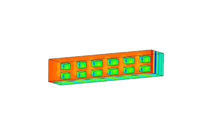
Refer to caption Refer to caption
a) FEM solution at t=1.5𝑡1.5t=1.5 b) FEM solution at t=1.8𝑡1.8t=1.8
Refer to caption Refer to caption
c) FEM/FDM solution at t=0𝑡0t=0 d) FEM/FDM solution at t=1.8𝑡1.8t=1.8
Figure 3: Isosurfaces of the simulated FEM/FDM solution of the model problem at different times: a), b) Test 1; c), d) Test 2.
Refer to caption Refer to caption
(a) Test 1. ω=50𝜔50\omega=50, σ=7%𝜎percent7\sigma=7\%, t=3𝑡3t=3 (b) Test 2. ω=60𝜔60\omega=60, σ=17%𝜎percent17\sigma=17\%, t=3𝑡3t=3
Refer to caption Refer to caption
(c) Test 1. ω=50𝜔50\omega=50, σ=7%𝜎percent7\sigma=7\%, t=3𝑡3t=3 (d) Test 2. ω=60𝜔60\omega=60, σ=17%𝜎percent17\sigma=17\%, t=3𝑡3t=3
Figure 4: a), b) Backscattered data of the one component, E2(x,t)subscript𝐸2𝑥𝑡E_{2}(x,t), of the electric field E(𝐱,t)𝐸𝐱𝑡E(\mathbf{x},t). c), d) Computed components E2subscript𝐸2E_{2} (below) and E1andE3subscript𝐸1andsubscript𝐸3E_{1}\ \text{and}\ E_{3} (on top) of the backscattered electric field E(𝐱,t)𝐸𝐱𝑡E(\mathbf{x},t).
Refer to caption Refer to caption
(a) maxΩFEMεr15subscriptsubscriptΩ𝐹𝐸𝑀subscript𝜀𝑟15\max\limits_{\Omega_{FEM}}\varepsilon_{r}\approx 15 (b) maxΩFEMμr2.5subscriptsubscriptΩ𝐹𝐸𝑀subscript𝜇𝑟2.5\max\limits_{\Omega_{FEM}}\mu_{r}\approx 2.5
Figure 5: Test 1. Computed images of reconstructed functions εr(𝐱)andμr(𝐱)subscript𝜀𝑟𝐱andsubscript𝜇𝑟𝐱\varepsilon_{r}(\mathbf{x})\ \text{and}\ \mu_{r}(\mathbf{x}) on a coarse mesh for ω=45𝜔45\omega=45, σ=7%𝜎percent7\sigma=7\%.
Refer to caption Refer to caption
(a) maxΩFEMεr14.9subscriptsubscriptΩ𝐹𝐸𝑀subscript𝜀𝑟14.9\max\limits_{\Omega_{FEM}}\varepsilon_{r}\approx 14.9 (b) maxΩFEMμr1.8subscriptsubscriptΩ𝐹𝐸𝑀subscript𝜇𝑟1.8\max\limits_{\Omega_{FEM}}\mu_{r}\approx 1.8
Figure 6: Test 1. Computed images of reconstructed functions εr(𝐱)andμr(𝐱)subscript𝜀𝑟𝐱andsubscript𝜇𝑟𝐱\varepsilon_{r}(\mathbf{x})\ \text{and}\ \mu_{r}(\mathbf{x}) on a 5 times adaptively refined mesh presented in Figure 8. Computations are done for ω=45𝜔45\omega=45, σ=7%𝜎percent7\sigma=7\%.
Refer to caption Refer to caption
(a) maxΩFEMεr15subscriptsubscriptΩ𝐹𝐸𝑀subscript𝜀𝑟15\max\limits_{\Omega_{FEM}}\varepsilon_{r}\approx 15 (b) maxΩFEMμr2.5subscriptsubscriptΩ𝐹𝐸𝑀subscript𝜇𝑟2.5\max\limits_{\Omega_{FEM}}\mu_{r}\approx 2.5
Refer to caption Refer to caption
(c) maxΩFEMεr14.9subscriptsubscriptΩ𝐹𝐸𝑀subscript𝜀𝑟14.9\max\limits_{\Omega_{FEM}}\varepsilon_{r}\approx 14.9 (d) maxΩFEMμr1.8subscriptsubscriptΩ𝐹𝐸𝑀subscript𝜇𝑟1.8\max\limits_{\Omega_{FEM}}\mu_{r}\approx 1.8
Figure 7: Test 1. Computed images of reconstructed functions εr(𝐱)andμr(𝐱)subscript𝜀𝑟𝐱andsubscript𝜇𝑟𝐱\varepsilon_{r}(\mathbf{x})\ \text{and}\ \mu_{r}(\mathbf{x}) in x2x3subscript𝑥2subscript𝑥3x_{2}x_{3} view: a), b) on a coarse mesh, c), d) on a 5 times adaptively refined mesh. Computations are done for ω=45𝜔45\omega=45, σ=7%𝜎percent7\sigma=7\%.
Refer to caption Refer to caption
(a) x1x2subscript𝑥1subscript𝑥2x_{1}x_{2}-view (b) x1x2subscript𝑥1subscript𝑥2x_{1}x_{2}-view
Refer to caption Refer to caption
(c) x1x3subscript𝑥1subscript𝑥3x_{1}x_{3}-view (d) x1x3subscript𝑥1subscript𝑥3x_{1}x_{3}-view
Refer to caption Refer to caption
(e) x2x3subscript𝑥2subscript𝑥3x_{2}x_{3}-view (f) x2x3subscript𝑥2subscript𝑥3x_{2}x_{3}-view
Figure 8: Different projections of 5 times adaptively refined meshes for computed images of Figures 6 (on the left) and Figures 10 (on the right), respectively.
Refer to caption Refer to caption
c) maxΩFEMεr15subscriptsubscriptΩ𝐹𝐸𝑀subscript𝜀𝑟15\max\limits_{\Omega_{FEM}}\varepsilon_{r}\approx 15 d)maxΩFEMμr2.2subscriptsubscriptΩ𝐹𝐸𝑀subscript𝜇𝑟2.2\max\limits_{\Omega_{FEM}}\mu_{r}\approx 2.2
Figure 9: Test 2. Computed images of reconstructed functions εr(𝐱)andμr(𝐱)subscript𝜀𝑟𝐱andsubscript𝜇𝑟𝐱\varepsilon_{r}(\mathbf{x})\ \text{and}\ \mu_{r}(\mathbf{x}) on a coarse mesh for ω=50𝜔50\omega=50, σ=17%𝜎percent17\sigma=17\%.
Refer to caption Refer to caption
(a) maxΩFEMεr14.4subscriptsubscriptΩ𝐹𝐸𝑀subscript𝜀𝑟14.4\max\limits_{\Omega_{FEM}}\varepsilon_{r}\approx 14.4 (b) maxΩFEMμr1.6subscriptsubscriptΩ𝐹𝐸𝑀subscript𝜇𝑟1.6\max\limits_{\Omega_{FEM}}\mu_{r}\approx 1.6
Figure 10: Test 2. Computed images of reconstructed functions εr(𝐱)andμr(𝐱)subscript𝜀𝑟𝐱andsubscript𝜇𝑟𝐱\varepsilon_{r}(\mathbf{x})\ \text{and}\ \mu_{r}(\mathbf{x}) on a 5 times adaptively refined mesh. Computations are done with ω=50𝜔50\omega=50, σ=17%𝜎percent17\sigma=17\%.
Refer to caption Refer to caption
(a) maxΩFEMεr15subscriptsubscriptΩ𝐹𝐸𝑀subscript𝜀𝑟15\max\limits_{\Omega_{FEM}}\varepsilon_{r}\approx 15 (b) maxΩFEMμr2.2subscriptsubscriptΩ𝐹𝐸𝑀subscript𝜇𝑟2.2\max\limits_{\Omega_{FEM}}\mu_{r}\approx 2.2
Refer to caption Refer to caption
(a) maxΩFEMεr14.4subscriptsubscriptΩ𝐹𝐸𝑀subscript𝜀𝑟14.4\max\limits_{\Omega_{FEM}}\varepsilon_{r}\approx 14.4 (b) maxΩFEMμr1.6subscriptsubscriptΩ𝐹𝐸𝑀subscript𝜇𝑟1.6\max\limits_{\Omega_{FEM}}\mu_{r}\approx 1.6
Figure 11: Test 2. Computed images of reconstructed functions εr(𝐱)andμr(𝐱)subscript𝜀𝑟𝐱andsubscript𝜇𝑟𝐱\varepsilon_{r}(\mathbf{x})\ \text{and}\ \mu_{r}(\mathbf{x}) in x2x3subscript𝑥2subscript𝑥3x_{2}x_{3} view: a), b) on a coarse mesh, c), d) on a 5 times adaptively refined mesh. Computations are done for ω=50𝜔50\omega=50, σ=17%𝜎percent17\sigma=17\%.

Acknowledgments

This research is supported by the Swedish Research Council (VR). The computations were performed on resources at Chalmers Centre for Computational Science and Engineering (C3SE) provided by the Swedish National Infrastructure for Computing (SNIC).

References

  • [1]
  • [2] F. Assous, P. Degond, E. Heintze and P. Raviart, On a finite-element method for solving the three-dimensional Maxwell equations, Journal of Computational Physics, 109 (1993), 222–237.
  • [3] A. Bakushinsky, M. Y. Kokurin, A. Smirnova, Iterative Methods for Ill-posed Problems, Inverse and Ill-Posed Problems Series 54, De Gruyter, 2011.
  • [4] L. Beilina and C. Johnson, A posteriori error estimation in computational inverse scattering, Mathematical Models in Applied Sciences, 1 (2005), 23-35.
  • [5] L. Beilina, Energy estimates and numerical verification of the stabilized Domain Decomposition Finite Element/Finite Difference approach for time-dependent Maxwell’s system, Central European Journal of Mathematics, 11 (2013), 702-733 DOI: 10.2478/s11533-013-0202-3.
  • [6] L. Beilina, Adaptive Finite Element Method for a coefficient inverse problem for the Maxwell’s system, Applicable Analysis, 90 (2011) 1461-1479.
  • [7] L. Beilina, M. Cristofol and K. Niinimäki, Optimization approach for the simultaneous reconstruction of the dielectric permittivity and magnetic permeability functions from limited observations, Inverse Problems and Imaging, 9 (1), pp. 1-25, 2015
  • [8] L. Beilina, N. T. Thành, M. V. Klibanov, J. Bondestam-Malmberg, Reconstruction of shapes and refractive indices from blind backscattering experimental data using the adaptivity, Inverse Problems, 30, 105007, 2014.
  • [9] L. Beilina, N. T. Thành, M. V. Klibanov, M. A. Fiddy, Reconstruction from blind experimental data for an inverse problem for a hyperbolic equation, Inverse Problems, 30 (2014), 025002.
  • [10] L. Beilina, M.V. Klibanov, Approximate global convergence and adaptivity for coefficient inverse problems, Springer, New-York, 2012.
  • [11] L. Beilina, M.V. Klibanov and M.Yu. Kokurin, Adaptivity with relaxation for ill-posed problems and global convergence for a coefficient inverse problem, Journal of Mathematical Sciences, 167, pp. 279-325, 2010.
  • [12] L. Beilina, M. Grote, Adaptive Hybrid Finite Element/Difference Method for Maxwell’s equations, TWMS Journal of Pure and Applied Mathematics, V.1(2), pp.176-197, 2010.
  • [13] M. Bellassoued, M. Cristofol, and E. Soccorsi, Inverse boundary value problem for the dynamical heterogeneous Maxwell’s system, Inverse Problems, (28), 095009, 2012.
  • [14] J. Bondestam Malmberg, A posteriori error estimate in the Lagrangian setting for an inverse problem based on a new formulation of Maxwell’s system, Inverse Problems and Applications, Springer Proceedings in Mathematics and Statistics , Vol. 120, 2015, pp. 42-53, 2015.
  • [15] J. Bondestam Malmberg, A posteriori error estimation in a finite element method for reconstruction of dielectric permittivity, arXiv:1502.07658, 2015.
  • [16] S. C. Brenner and L. R. Scott, The Mathematical Theory of Finite Element Methods (2nd edn), Springer-Verlag, New York, 2002.
  • [17] P. Ciarlet, Jr. and J. Zou, Fully discrete finite element approaches for time-dependent Maxwell’s equations, Numerische Mathematik 82 (1999), 193-219.
  • [18] P. Ciarlet, Jr., H. Wu and J. Zou, Edge element methods for Maxwell’s equations with strong convergence for Gauss’ laws, SIAM Journal on Numerical Analysis 52 (2014), 779-807.
  • [19] R. Courant, K. Friedrichs and H. Lewy On the partial differential equations of mathematical physics, IBM Journal of Research and Development, 11 (1967), 215-234.
  • [20] G. C. Cohen, Higher order numerical methods for transient wave equations, Springer-Verlag, 2002.
  • [21] A. Elmkies and P. Joly, Finite elements and mass lumping for Maxwell’s equations: the 2D case. Numerical Analysis, 324 (1997), 1287–1293.
  • [22] H. W. Engl, M. Hanke and A. Neubauer, Regularization of Inverse Problems Boston: Kluwer Academic Publishers, 2000.
  • [23] B. Engquist and A. Majda, Absorbing boundary conditions for the numerical simulation of waves, Mathematics of Computation, 31 (1977), 629-651.
  • [24] H. Feng, D. Jiang and J. Zou, Simultaneous identification of electric permittivity and magnetic permeability, Inverse Problems, 26 (2010), 095009.
  • [25] D. W. Einters, J. D. Shea, P. Komas, B. D. Van Veen and S. C. Hagness Three-dimensional microwave breast imaging: Dispersive dielectric properties estimation using patient-specific basis functions IEEE Transactions on Medical Imaging 28 (2009), 969–981
  • [26] K. Eriksson, D. Estep and C. Johnson, Calculus in Several Dimensions, Springer, Berlin, 2004.
  • [27] K Ito, B Jin, and T Takeuchi Multi-parameter Tikhonov regularization, Methods and Applications of Analysis, 18 (2011), 31–46.
  • [28] C. Johnson and A. Szepessy, Adaptive finite element methods for conservation laws based on a posteriori error estimation, Comm. Pure Appl. Math., 48, 199–234, 1995.
  • [29] C. Johnson, Numerical Solution of Partial Differential Equations by the Finite Element Method, Dover Books on Mathematics, 2009.
  • [30] M.V. Klibanov, A.B. Bakushinsky and L. Beilina, Why a minimizer of the Tikhonov functional is closer to the exact solution than the first guess, J. Inverse and Ill-Posed Problems, 19, 83-105, 2011.
  • [31] O. A. Ladyzhenskaya, Boundary Value Problems of Mathematical Physics, Springer Verlag, Berlin, 1985.
  • [32] C. D. Munz, P. Omnes, R. Schneider, E. Sonnendrucker and U. Voss, Divergence correction techniques for Maxwell Solvers based on a hyperbolic model, Journal of Computational Physics, 161 (2000), 484–511.
  • [33] O. Pironneau, Optimal shape design for elliptic systems, Springer-Verlag, Berlin, 1984.
  • [34] N. T. Thành, L. Beilina, M. V. Klibanov, M. A. Fiddy, Reconstruction of the refractive index from experimental backscattering data using a globally convergent inverse method, SIAM J. Scientific Computing,36 (3) (2014), 273-293.
  • [35] S. Hosseinzadegan, Iteratively regularized adaptive finite element method for reconstruction of coefficients in Maxwell’s system, Master’s Thesis in Applied Mathematics, Department of Mathematical Sciences, Chalmers University of Technology and Gothenburg University, 2015.
  • [36] L. R. Scott, S. Zhang, Finite element interpolation of nonsmooth functions satisfying boundary conditions, Math.Comp., 54 (1990), 483–493.
  • [37] D. R. Smith, S. Schultz, P. Markos and C. M. Soukoulis, Determination of effective permittivity and permeability of metamaterials from reflection and transmission coefficients, Physical Review B, 65 (2002), DOI:10.1103/PhysRevB.65.195104.
  • [38] PETSc, Portable, Extensible Toolkit for Scientific Computation, http://www.mcs.anl.gov/petsc/.
  • [39] A.N. Tikhonov, A.V. Goncharsky, V.V. Stepanov and A.G. Yagola, Numerical Methods for the Solution of Ill-Posed Problems, London: Kluwer, London, 1995.
  • [40] Tikhonov A.N., Goncharskiy A.V., Stepanov V.V., Kochikov I.V. Ill-posed problems of the image processing, DAN USSR, 294, № 4. 832-837, 1987.
  • [41] WavES, the software package, http://www.waves24.com
  • [42] X. Zhang, H. Tortel, S. Ruy and A. Litman Microwave imaging of soil water diffusion using the linear sampling method, IEEE Geoscience and Remote Sensing Letters 8 (2011),421–425