Optimizing the StackSlide setup and data selection for continuous-gravitational-wave searches in realistic detector data

Abstract

The search for continuous gravitational waves in a wide parameter space at fixed computing cost is most efficiently done with semicoherent methods, e.g. StackSlide, due to the prohibitive computing cost of the fully coherent search strategies. Prix&Shaltev Prix and Shaltev (2012) have developed a semi-analytic method for finding optimal StackSlide parameters at fixed computing cost under ideal data conditions, i.e. gap-less data and constant noise floor. In this work we consider more realistic conditions by allowing for gaps in the data and changes in noise level. We show how the sensitivity optimization can be decoupled from the data selection problem. To find optimal semicoherent search parameters we apply a numerical optimization using as example the semicoherent StackSlide search. We also describe three different data selection algorithms. Thus the outcome of the numerical optimization consists of the optimal search parameters and the selected dataset. We first test the numerical optimization procedure under ideal conditions and show that we can reproduce the results of the analytical method. Then we gradually relax the conditions on the data and find that a compact data selection algorithm yields higher sensitivity compared to a greedy data selection procedure.

I Introduction

The enormous computational requirement of the wide parameter-space searches for continuous gravitational waves impose a cautious use of the available computing resources, as we always aim at maximal sensitivity . In this respect to maximize the sensitivity of a semicoherent search, for example StackSlide Brady and Creighton (2000); Cutler et al. (2005), means that we need to choose the optimal search parameters, namely number of segments, segment duration and optimal maximal mismatch on the coarse and fine grid. How to do this at fixed computing cost for a single astrophysical target and under the ideal conditions of constant noise floor and data without gaps has been studied in Prix and Shaltev (2012), where analytical expressions have been derived to determine the optimal search parameters. In Ref. Ming et al. (2015), while still assuming ideal conditions on the data, a framework to distribute the total available computing cost between different possible targets based on astrophysical priors has been developed. However under realistic conditions the available data, as collected for example from the Laser Interferometer Gravitational-Wave Observatory (LIGO) Abbott et al. (2009a); Aasi et al. (2015a), can be fragmented, e.g., due to down-time of the detectors, and there might be variations in the noise floor. The fragmentation of the data can significantly affect the computing cost function and thus the optimal search parameters. On the other hand, the noise fluctuations suggest the use of a data selection procedure in order to spend the available computing cycles searching data of higher quality.

In this work we extend Ref. Prix and Shaltev (2012) to these more realistic conditions by taking into account possible gaps in the data and noise level changes. First we show, how the real conditions manifest in the sensitivity function. Then we reformulate the problem, such that a numerical optimization procedure can be applied to find optimal semicoherent search parameters. We also describe a suitable data selection algorithm. The outcome of the proposed numerical optimization are the optimal search parameters and the selected data, so that the search can be performed in practice. We first test the numerical optimization procedure under ideal conditions and obtain the results of the analytical method proposed in Ref. Prix and Shaltev (2012). Then we give examples of practical application.

This paper is organized as follows. In Sec. II we introduce the ingredients of the search-optimization method, i.e., the threshold signal-to-noise ratio (SNR), the sensitivity function, and the computing cost function. The numerical optimization of the search parameters and in particular the data selection method are described in Sec. III. In Sec. IV we give examples of practical application and discuss in Sec. V.

Notation

We use tilde when referring to fully coherent quantities, $\widetilde{Q}$, and overhat when referring to semicoherent quantities, $\widehat{Q}$.

II Threshold SNR, sensitivity function and computing cost

In this section we introduce the main ingredients needed to define the optimization problem, i.e., to find the number of segments $N$ with segment duration $\Delta T$ and coarse and fine grid mismatch, $\widetilde{m}$ resp. $\widehat{m}$, which maximize the sensitivity of the search at fixed computing cost $C_{0}$. These ingredients are the threshold SNR required for detection, the sensitivity function, which we want to maximize, and the computing cost function.

II.1 Threshold SNR

A claim for detection when searching for a signal, in particular a weak signal, in the presence of noise is sensible only in the context of two well defined quantities. The first one, called false-alarm probability, is the probability to falsely claim a detection when the signal is not present in the data. The second quantity, called false-dismissal probability, is the probability to miss the signal even if the signal is indeed present in the data.

When a signal is present in the data the semicoherent StackSlide statistic follows a non-central $\chi^{2}$ distribution with $4N$ degrees of freedom. Using the definitions of Prix and Shaltev (2012), we denote this by $\chi^{2}_{4N}(\hat{\mathcal{F}},\hat{\rho}^{2})$, where $\hat{\rho}^{2}$ is the non-centrality parameter, i.e., the sum of the squared SNR of the individual segments $\hat{\rho}^{2}\equiv\sum_{i=1}^{N}\widetilde{\rho}^{2}_{i}$. We can integrate the false-alarm probability

$$p_{\mathrm{fA}}(\hat{\mathcal{F}}_{\mathrm{th}})=\int_{\hat{\mathcal{F}}_{\mathrm{th}}}^{\infty}\mathrm{d}\hat{\mathcal{F}}\,\chi_{4N}^{2}(\hat{\mathcal{F}};0)\ ,$$ (1)

and by inversion for a given false-alarm $p_{\mathrm{fA}}^{*}$ obtain the threshold $\hat{\mathcal{F}}_{\mathrm{th}}$. For a pre-defined false-dismissal $p_{\mathrm{fD}}^{*}$ probability

$$p_{\mathrm{fD}}(\hat{\mathcal{F}}_{\mathrm{th}},\hat{\rho}^{2})=\int_{-\infty}^{\hat{\mathcal{F}}_{\mathrm{th}}}\mathrm{d}\hat{\mathcal{F}}\,\chi^{2}_{4N}(\hat{\mathcal{F}};\hat{\rho}^{2})\ ,$$ (2)

using $\hat{\mathcal{F}}_{\mathrm{th}}$ we aim to obtain the critical non-centrality

$$\hat{\rho}^{*2}=\hat{\rho}^{2}(p_{\mathrm{fA}}^{*},p_{\mathrm{fD}}^{*},N)\ ,$$ (3)

and thus the threshold SNR.

The computation of the critical non-centrality $\hat{\rho}^{*2}$ is complicated by the fact that for wide parameter-space searches the right-hand side of Eq. (2) requires averaging over sky position and polarization parameters of the signal carried out at fixed intrinsic amplitude $h_{0}$. In Ref. Prix and Shaltev (2012) for example, a signal population of constant SNR has been assumed. Therefore by application of the central limit theorem and approximation of the $\chi^{2}$ distribution by a Gaussian distribution, Eq. (2) has been analytically integrated and inverted to obtain (3). For weak signals and large number of segments (see Fig. 2 in Ref. Prix and Shaltev (2012)) this results in the “weak-signal Gauss (WSG) approximation” for the critical non-centrality parameter

$$\hat{\rho}^{*2}(p_{\mathrm{fA}}^{*},p_{\mathrm{fD}}^{*},N)\approx 2\sqrt{4N}(\mathrm{erfc}^{-1}(2p_{\mathrm{fA}}^{*})+\mathrm{erfc}^{-1}(2p_{\mathrm{fD}}^{*}))\ .$$ (4)

With this we define the per-segment threshold SNR

$$\rho^{*}\equiv\sqrt{\frac{\hat{\rho}^{*2}(p_{\mathrm{fA}}^{*},p_{\mathrm{fD}}^{*},N)}{N}}\ .$$ (5)

Recently a new semi-analytical method has been developed to estimate the sensitivity of a search Wette (2012). In this method the assumption of signal distribution of constant SNR has been relaxed, where a semi-analytical approximation for the computation of an isotropic threshold SNR has been introduced. We refer to this method as the KWS approximation. In the KWS approximation the averaged over segments threshold $\rho^{*}$ is obtained recursively. At iteration $i$ the value of $\rho^{*}$ is

$$\rho=F\big{(}\rho\big{)}\ ,$$ (6)

where

$$\rho_{i+1}=F\left(\frac{\rho_{i}+\rho_{i-1}}{2}\right)\ .$$ (7)

For the details required to implement the method in practice see Wette (2012). The accuracy of this technique is within the calibration error of the gravitational-wave detector with results similar to the sensitivity estimates performed with Monte-Carlo methods, thus we adopt it in the following numerical optimization scheme Abadie et al. (2010a); Wette (2012).

II.2 Sensitivity function

The signal strength $h_{\mathrm{rms}}$ in the detector, depends on the intrinsic amplitude $h_{0}$, the sky-position of the source, the polarization angles and the detector orientation. Averaging isotropically over the sky-position and polarization yields

$$\left\langle h_{\mathrm{rms}}^{2}\right\rangle_{\mathrm{sky,pol}}=\frac{2}{25}h_{0}^{2}\ .$$ (8)

Under ideal conditions of data without gaps with duration $T$ and constant noise floor $S_{n}$ the accumulated squared $\mathrm{SNR}$ in a semicoherent search is Prix and Shaltev (2012):

$$\hat{\rho}^{2}=2[1-\xi(\widetilde{m}+\widehat{m})]\frac{2N_{\mathrm{det}}}{S_{n}}h_{\mathrm{rms}}^{2}T\ ,$$ (9)

where $\xi\in(0,1)$ is the geometrical factor used to estimate the average mismatch of the template bank, $\widetilde{m}$ is the mismatch on the coarse grid, $\widehat{m}$ is the mismatch on the fine grid and $N_{\mathrm{det}}$ is the number of detectors. Typically, the data is made available in the form of $N_{\mathrm{SFT}}$ number of Short Fourier Transforms (SFTs) of duration $T_{\mathrm{SFT}}$. To take into account possible noise floor fluctuations, the noise floor can be written as Prix and Wette (2012)

$$\mathcal{S}^{-1}(f_{0})\equiv N_{\mathrm{SFT}}^{-1}\sum_{n=1}^{N_{\mathrm{SFT}}}S_{n}^{-1}(f_{0})\ ,$$ (10)

where $S_{n}$ is the per SFT noise Power Spectral Density (PSD) estimated at frequency $f_{0}$. To account for the possible gaps in the data we define the actual amount of available data

$$T_{\mathrm{data}}\equiv N_{\mathrm{SFT}}T_{\mathrm{SFT}}\ .$$ (11)

Using Eqs. (8), (10) and (11) we can rewrite Eq. (9) to obtain the accumulated squared $\mathrm{SNR}$ in a semicoherent search under realistic conditions, namely

$$\left\langle\hat{\rho}^{2}\right\rangle_{\mathrm{sky,pol}}=\frac{4}{25}[1-\xi(\widetilde{m}+\widehat{m})]h_{0}^{2}T_{\mathrm{data}}\mathcal{S}^{-1}\ .$$ (12)

To estimate the minimal detectable intrinsic amplitude $h_{0}$ at fixed false-alarm $p_{\mathrm{fA}}^{*}$ and false-dismissal $p_{\mathrm{fD}}^{*}$ probability we use the per-segment threshold SNR $\rho^{*}$. With $\left\langle\hat{\rho}^{2}\right\rangle_{\mathrm{sky,pol}}\equiv N\rho^{*2}$ substitution in Eq. (12) and rearrangement yields

$${h_{0}}=\frac{5}{2}[1-\xi(\widetilde{m}+\widehat{m})]^{-1/2}\rho^{*}\sqrt{N}\sqrt{\frac{1}{\mathcal{G}}}\ ,$$ (13)

where

$$\mathcal{G}\equiv T_{\mathrm{data}}\mathcal{S}^{-1}$$ (14)

is the goodness of the data. Eq. (13) is the function that we need to minimize under the constraint of fixed computing cost $C_{0}$ in order to maximize the sensitivity of the search.

II.3 Computing cost

The total computing cost $C_{\mathrm{tot}}(\widetilde{m},\widehat{m},N,\Delta T,N_{\mathrm{SFT}})$ of the StackSlide method is composed by the cost $\widetilde{C}(\widetilde{m},\Delta T,N_{\mathrm{SFT}})$ to compute the $\mathcal{F}$-statistic Jaranowski et al. (1998b); Cutler and Schutz (2005) on the coarse grid and the cost $\widehat{C}(\widehat{m},N,\Delta T)$ to sum these $\mathcal{F}$-statistic values across all segments on the fine grid, thus

$$C_{\mathrm{tot}}(\widetilde{m},\widehat{m},N,\Delta T,N_{\mathrm{SFT}}) = \widetilde{C}(\widetilde{m},\Delta T,N_{\mathrm{SFT}})$$ (15)

$$+ \widehat{C}(\widehat{m},N,\Delta T)\ .$$

The computing cost of the coherent step using the SFT method is

$$\widetilde{C}(\widetilde{m},\Delta T,N_{\mathrm{SFT}})=N_{\mathrm{SFT}}\widetilde{\mathcal{N}}(\widetilde{m},\Delta T)\widetilde{c}_{0}^{SFT}\ ,$$ (16)

where $\widetilde{\mathcal{N}}(\widetilde{m},\Delta T)$ is the number of coarse-grid templates and $\widetilde{c}_{0}^{SFT}$ is an implementation- and hardware-dependent fundamental computing cost. Similarly, the incoherent computing cost is

$$\widehat{C}(\widehat{m},N,\Delta T)=N\widehat{\mathcal{N}}(\widehat{m},\Delta T,N)\widehat{c}_{0}\ ,$$ (17)

where $\widehat{\mathcal{N}}(\widehat{m},\Delta T,N)$ is the number of fine-grid templates and $\widehat{c}_{0}$ is the fundamental cost of adding $\mathcal{F}$-statistic values.

II.4 Templates counting

The general expression for the number of templates required to cover some parameter space $\mathbb{P}$ is

$$\mathcal{N}=\theta_{n}\,m^{-n/2}\,\mathcal{V}_{n}\,,\quad\mbox{with}\quad\mathcal{V}_{n}\equiv\int_{\mathbb{T}_{n}}\mathrm{d}^{n}\lambda\,\sqrt{\det g}\,,$$ (18)

where $\theta_{n}$ is the normalized thickness of the search grid, $m$ is the maximal-mismatch, $\det g$ is the determinant of the parameter-space metric $g_{ij}$ and $\mathcal{V}_{n}$ is the metric volume of the $n$-dimensional space of the template bank. For hyper-cubic lattice the normalized thickness is $\theta_{\mathbb{Z}_{n}}=n^{n/2}\,2^{-n}$, while for an $A^{*}$ lattice it is $\theta_{A^{*}_{n}}=\sqrt{n+1}\left\{\frac{n(n+2)}{12(n+1)}\right\}^{n/2}$ Prix (2007). The choice of the dimensionality of the template bank is subject to the maximization of the number of templates, namely

$$\widetilde{\mathcal{N}}_{{\widetilde{n}}}=\max_{n}\widetilde{\mathcal{N}}_{n}\,,\quad\mbox{and}\quad\widehat{\mathcal{N}}_{{\widehat{n}}}=\max_{n}\widehat{\mathcal{N}}_{n}\,.$$ (19)

In Ref. Prix and Shaltev (2012) we used the factorization of the semicoherent metric volume

$$\widehat{\mathcal{V}}_{\widehat{n}}(N,\Delta T)=\gamma_{{\widehat{n}}}(N)\,\widetilde{\mathcal{V}}_{\widehat{n}}(\Delta T)\,,$$ (20)

to derive the general power-law computing-cost model, as in the gap-less data case, the refinement factor $\gamma_{{\widehat{n}}}(N)$ is only a function of the number of segments $N$. However using real data introduces an additional dependency on the time span of the search through the actual position of the segments in time. For details see, e.g., Pletsch (2010). We aim to model the real conditions as closely as possible, therefore in the numerical optimization we directly compute the semicoherent metric

$$\widehat{g}(t_{\mathrm{ref}})=\frac{1}{N}\sum_{i=1}^{N}\widetilde{g_{i}}(t_{i},\Delta T,t_{\mathrm{ref}})\ ,$$ (21)

where $\widetilde{g}_{i}(t_{i},\Delta T,t_{\mathrm{ref}})$ is the coherent metric of segment $i$ at fixed reference time $t_{\mathrm{ref}}$. To compute the coherent metric $\widetilde{g}_{i}(t_{i},\Delta T,t_{\mathrm{ref}})$ in this work we use the analytical expressions found in Ref. Pletsch (2010).

II.5 The choice of spindown parameter space

The choice of the dimensionality of the template bank through Eqs. (19) is possible only for a simple rectangular geometry of the parameter space.

Using the spindown age of a potential source Brady and Creighton (2000):

$$\tau=f/|\dot{f}|\ .$$ (22)

the spindown search band in dimension $k$ is

$$|f^{(k)}|\leq k!\frac{f}{\tau^{k}}\ .$$ (23)

This however means that the spindown band is frequency dependent, which may be impractical. Therefore if we keep the number of templates in the spindown space constant by fixing a minimal detectable spindown age $\tau_{0}$ at some frequency $f_{0}$, the detectable spindown age at frequency $f$ yields

$$\tau(f)=\tau_{0}f/f_{0}\ .$$ (24)

This would define the simplest possible parameter-space volume for optimization, namely a “box”.

A more complicated triangular parameter-space shape has been discussed in Ref. Wette et al. (2008) and used in the search for gravitational waves from the supernova remnant Cassiopeia-A Abadie et al. (2010b). The parameters of a search over such space are difficult to optimize as the spindown order may vary even in infinitesimally small slices of a frequency band. In the present work we neglect this fact in order to compare the outcome of the optimization with previously obtained results.

III Numerical optimization procedure for a semicoherent StackSlide search with a fixed frequency band

(a) Greedy data selection for requested $N=10$ segments with duration $\Delta T=3$ time units. Note how segments 8, 9 and 10 overlap in time with their neighboring segments, however they do not share data. This is depicted by the black fill of the segments.

(b) Compact data selection for requested $N=2$ segments with duration $\Delta T=3$ time units. We show only the best segment combination. For comparison with the greedy data selection method we denoted the selected segments of the greedy procedure with G. The PSD of the SFTs has been chosen such that the best segment combination of the compact method has much shorter time span.

Figure 1: Schematic representation of (a) greedy and (b) compact data selection. The middle line of squares in gray are the available SFTs of unit time, where the number inside the square denotes the PSD. The white squares without a number are gaps in the data. The selected segments are the white rectangles, where the number inside is the number of the segment.

In this section we consider the practical implementation of a numerical optimization procedure to find optimal search parameters for a semicoherent StackSlide search.

III.1 Definition of the optimization problem

To maximize the sensitivity of the search, i.e., to minimize the measurable intrinsic amplitude, we need to minimize the function given in Eq. (13), namely:

$$h_{0}(\widetilde{m},\widehat{m},N,\mathcal{G})=\frac{5}{2}[1-\xi(\widetilde{m}+\widehat{m})]^{-1/2}\rho^{*}\sqrt{N}\sqrt{\frac{1}{\mathcal{G}}}$$ (25)

under the constraints

$$C_{\mathrm{tot}} \leq C_{0}\ ,$$

$$0< \widetilde{m} <1\ ,$$

$$0< \widehat{m} <1\ ,$$

$$\widetilde{\mathcal{N}} \leq \widehat{\mathcal{N}}\ ,$$ (26)

where $C_{0}$ is a given maximal available computing cost. Note that in practice the cost constraint is difficult to be fulfilled as an equality, however a reasonable algorithm should find a solution for which $C_{\mathrm{tot}}$ becomes approximately $C_{0}$. In order to minimize $h_{0}$ we need a data selection procedure which maximizes the goodness of the data $\mathcal{G}$. Through the data selection procedure we can transform the implicit dependency of Eq. (25) on the segment duration $\Delta T$ into an explicit dependency and minimize the 4D optimization problem $h_{0}(\widetilde{m},\widehat{m},N,\Delta T)$.

III.2 Data selection

For a given amount of data and requested number of segments of some duration, we need an algorithm to select the data which maximizes the goodness $\mathcal{G}$, i.e., pick as much data $T_{\mathrm{data}}$ as possible of lowest noise level $\mathcal{S}$ as possible . This would require computation of all possible segment combinations, their ranking by the goodness $\mathcal{G}$ and selection of the first segment realization which satisfies the computing cost constraint. For the simple case of picking $k$ non-overlapping segments out of $n$ possible, without replacement and ordering, the number of combinations is given by the well known binomial coefficient formula

$$\left(\begin{tabular}[]{c}$n$\\ $k$\end{tabular}\right)=\frac{n!}{k!(n-k)!}\,.$$ (27)

For example, having 200 days of available data, choosing 100 segments of 1 day duration, yields roughly $9\times 10^{58}$ possible combinations. Clearly such data selection procedure is not well suited for practical implementation . Therefore we consider three different suboptimal, but computationally feasible, alternative methods for data selection. Namely the two extremes, a greedy method and a compact method, and a third procedure greedy-compact, which is placed somewhere in between, in terms of the total observation time.

III.2.1 A greedy method

For requested $N$ number of segments with duration $\Delta T$ and given set of SFTs with duration $T_{\mathrm{SFT}}$, which are ordered in time by increasing timestamps $t_{j}$, within a greedy data selection we always pick the segments with the maximal goodness. The steps of the algorithm are (pseudo code is given in Alg. 1)

1. For each timestamp $t_{j}$ find all SFTs in the time interval $[t_{j},t_{j}+\Delta T]$ and compute $\mathcal{G}_{j}$.

2. Select the segment starting from $t_{j}$ such that $\mathcal{G}_{j}$ is maximal and remove the timestamps of the SFTs, which belong to the selected segment.

3. Repeat steps 1. and 2. until $N$ segments are selected or there is no more data left.

An example of data selection is schematically presented in Fig. 1(a), where we select $N=10$ segments of duration $\Delta T=3$ time units out of data set with $N_{\mathrm{SFT}}=33$ SFTs of unit time distributed in $T=37$ time units. Three of the selected segments overlap in time with their neighbors, however these overlapping segments do not share data. Such partial segments suggest grid construction based on the actual length of the segments instead of the maximal length $\Delta T$, which would reduce the coherent part of the total computing cost in these cases. However this would complicate the combination of the $\mathcal{F}$-statistic values in the semicoherent step of the StackSlide search, thus the overall effect remains unclear. Therefore we stick to a constant grid for every segment. While the above criticism also holds for the other two data selection methods proposed in this subsection, we should note a specific weak point of the greedy algorithm. Namely, depending on the quality of the data this method tends to maximize the total observation time of the generated segment list, for example when the data is of low noise level at the beginning and at the end, but contains disturbences or gaps in the middle. In such cases an alternative method yielding more compact segment list may lead to higher search sensitivity.

Before proceeding with the explanation of the compact data selection, we note, that an equivalent procedure of the greedy method has been used to select data for the recent all-sky Einstein@Home searches for continuous gravitational waves in LIGO S6 data EAH (2015).

III.2.2 A compact method

For requested $N$ number of segments with duration $\Delta T$ and given set of SFTs with duration $T_{\mathrm{SFT}}$, which are ordered in time by increasing timestamps $t_{j}$, the compact data selection aims to maximize the goodness while keeping the total timespan of the data close to the minimum $N\Delta T$. The algorithm consist in the following steps (pseudo code is given in Alg. 2)

1. Set the start time of the first segment to $t_{s}=t_{j}$.

2. Find all SFTs in the time interval $[t_{s},t_{s}+\Delta T]$.

3. Update $t_{s}$ with the first $t_{j}\geq t_{s}+\Delta T$.

4. Repeat steps 2. and 3. until N segments are selected or there is no more data left.

5. Compute $\mathcal{G}_{j}$.

6. Repeat steps 1. to 5. for all timestamps $t_{j}$.

7. Sort all found combinations by decreasing $\mathcal{G}$.

Using the compact method of data selection, we obtain a list of possible segment combinations. Then we use the first combination, which satisfies the computing cost constraint. An example of compact data selection is schematically presented in Fig. 1(b), where we select $N=2$ segments of duration $\Delta T=3$ time units out of data set with $N_{\mathrm{SFT}}=33$ SFTs of unit time distributed in $T=37$ time units. For comparison with the greedy method we also show the outcome of the greedy procedure. This example is specially constructed to stress the difference between the compact and the greedy method in terms of the time spanned by the data.

Due to the complexity of the compact method, but also to fill the gap to the greedy data selection algorithm, we also consider a third method, namely a greedy-compact algorithm.

III.2.3 A greedy-compact method

This method lies between the greedy and the compact methods in terms of the total span of the selected data. We achieve that by maximization of the sensitivity per cost ratio $h_{0}^{-1}/C$. Using Eq. (25) this is equivalent to maximization of the ratio $\mathcal{G}/C^{2}$. The steps of the algorithm are (see Alg. 3 for pseudo code)

1. For each timestamp $t_{j}$ find all SFTs in the time interval $[t_{j},t_{j}+\Delta T]$ and compute $\mathcal{G}_{j}/C_{j}^{2}$, where $C_{j}$ is the computing cost resulting from using this particular segment list and $C_{1}=1$.

2. Select the segment starting from $t_{j}$ such that $\mathcal{G}_{j}/C_{j}^{2}$ is maximal and remove the timestamps of the SFTs, which belong to the selected segment.

3. Repeat steps 1. and 2. until $N$ segments are selected or there is no more data left.

In the next section we compare the results of the optimization procedure using the three different data selection methods.

IV Examples of practical application

In the absence of direct detection limits on the intrinsic gravitational-wave amplitude have been set for example, in Refs. Abbott et al. (2008, 2009b); Aasi et al. (2013a); Abbott et al. (2010); Aasi et al. (2013b, 2015b) The intrinsic gravitational-wave amplitude and with this the probability of detection depends on unknown priors, in particular on the population and ellipticity of the continuous waves emitters. Thorough population studies and prospects for detection with the initial and Advanced LIGO Aasi et al. (2015c) detectors can be found in Refs. Palomba (2005); Knispel and Allen (2008); Wade et al. (2012). In this work it is convenient to use as a figure of merit the sensitivity depth

$$\mathcal{D}=\frac{\sqrt{\mathcal{S}}}{h_{0}}\,,$$ (28)

a quantity introduced in Ref. Behnke et al. (2015). With this we use for comparison the analytical solution found in the “Directed search for Cassiopeia-A“ example in Ref. Prix and Shaltev (2012), therefore we use the same search volume enclosed in the frequency band $f\in[100,300]\,\mathrm{Hz}$ with spindown ranges corresponding to a spindown age $\tau_{\min}=300\,\mathrm{y}$. The computing cost constraint is $C_{0}\approx 472$ days on a single computing core, where the fundamental computing constants are

$$\widetilde{c}_{0}^{\mathrm{SFT}}=7\times 10^{-8}\ \mathrm{s},\ \ \ \ \widehat{c}_{0}=6\times 10^{-9}\ \mathrm{s}\ .$$ (29)

In the following we assume an $A^{*}$ search grid, for which $\xi\approx 0.5$. We fix the false-alarm $p_{\mathrm{fA}}=1\times 10^{-10}$ and false-dismissal probability $p_{\mathrm{fD}}=0.1$. The weakest detectable signal, as estimated for $T_{\mathrm{data}}=0.7\times 2\times 12\,\mathrm{days}$, $\xi=0.5$ and $\widetilde{m}=0.2$ yields sensitivity depth of

$$\left.\mathcal{D}\right|_{\mathrm{opt}}\approx 54.4\,\mathrm{Hz}^{-1/2}\,,$$ (30)

which in the KWS approximation yields

$$\left.\mathcal{D}^{{\mathrm{KWS}}}\right|_{\mathrm{opt}}\approx 36.9\,\mathrm{Hz}^{-1/2}\,.$$ (31)

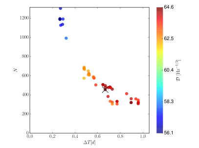
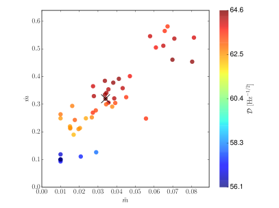
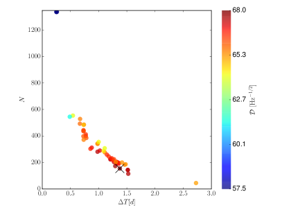
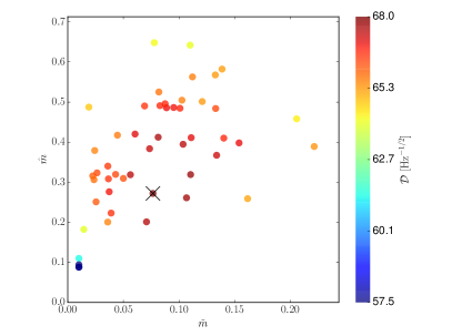
We perform the numerical optimization with the NOMAD Le Digabel (2011) implementation of a Mesh Adaptive Direct Search (MADS) Audet and E (2004); Abramson et al. (2009); Conn and Digabel (2011) algorithm for constrained derivative-free optimization. For each of the following examples we run the procedure 50 times from a common initial starting point:

$$N_{0}=200\,,\quad\Delta T_{0}=1\,\mathrm{days}\,$$

$$\widetilde{m}_{0}=0.5\,,\quad\widehat{m}_{0}=0.5,$$

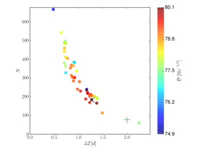
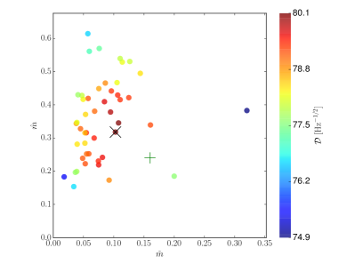
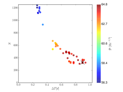
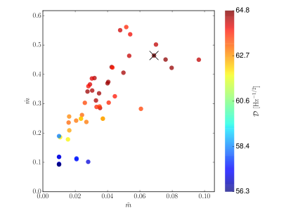
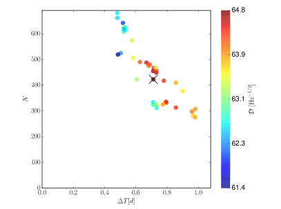
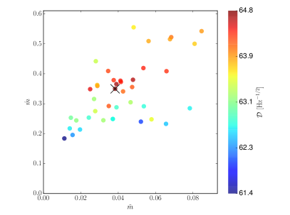
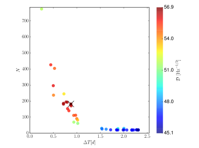
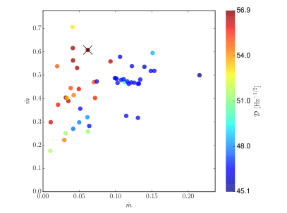
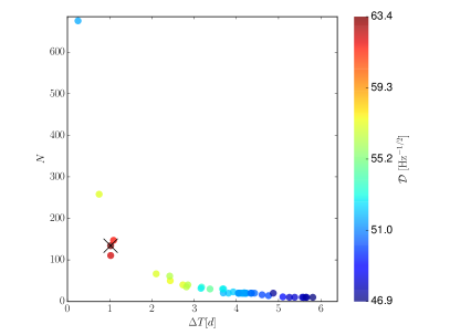
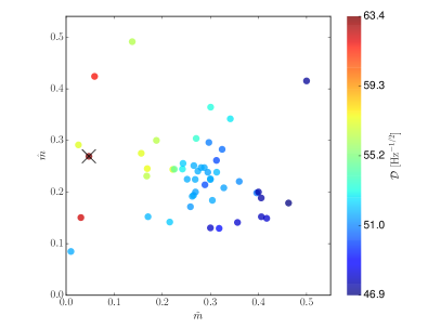
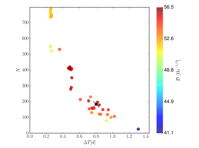
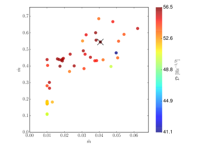
while we use different mesh coarsening and mesh update basis parameters . We use these multiple runs of the optimization effectively to escape local extremes. Note that in Figures 2 to 6 we plot the best solution from each of these 50 runs, however on average approximately $17\times 10^{3}$ points have been evaluated per data selection algorithm for each of the studied cases.

In all cases we use the three different data selection algorithms.

IV.1 Directed search using simulated data

Gapless data with constant noise floor

We first consider optimization using simulated data from 2 detectors spanning 365 days, without gaps, and with a constant noise floor $\sqrt{S_{\mathrm{n}}}=1\ \mathrm{Hz}^{-1/2}$. Using the analytical optimization method discussed in Prix and Shaltev (2012) and the WSG approximation to obtain optimal parameters, the sensitivity depth of the search expressed in the KWS approximation is

$$\left.\mathcal{D}^{{\mathrm{KWS}}}\right|_{\mathrm{opt}}\approx 78.6\,\mathrm{Hz}^{-1/2}\ .$$ (32)

The optimal maximal mismatch on the coarse and fine grid is

$$\begin{split}{\widetilde{m}}_{\mathrm{opt}}=0.16\,,&\quad{\widehat{m}}_{\mathrm{opt}}=0.24\ ,\end{split}$$ (33)

and the optimal number of segments ${N}_{\mathrm{opt}}$, segment duration ${\Delta T}_{\mathrm{opt}}$ and total observation time ${T}_{\mathrm{opt}}$ are

$$\begin{split}{N}_{\mathrm{opt}}=76.5\,,&\quad{\Delta T}_{\mathrm{opt}}\approx 2.0\,\mathrm{days}\,,\\ {T}_{\mathrm{opt}}&\approx 155.5\,\mathrm{days}\,.\end{split}$$ (34)

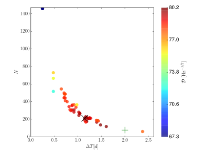
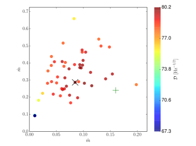
The results of the numerical optimization performed with the three different data selection algorithms are plotted in Fig. 2. In Table 1 we summarize the found optimal solutions. The three data selection methods in this case lead to equal sensitivity, which is expected, given that the data is ideal, i.e., of constant noise floor and without gaps. The small deviation in the optimal found parameters is due to the usage of the numerical optimization method.

Using the more accurate KWS method, the gain in sensitivity of this toy semicoherent search compared to the original fully coherent search is approximately $2.2\$.

	greedy	compact	greedy-compact
$\mathcal{D}\,[\mathrm{Hz}^{-1/2}]$	$80.2$	$80.1$	$80.1$
$T\,[\mathrm{d}]$	245	253.8	239.3
$N$	210	203	184.1
$\Delta T\,[\mathrm{d}]$	1.1	1.2	1.3
$\widetilde{m}$	0.08	0.09	0.10
$\widehat{m}$	0.29	0.37	0.32

Table 1: Optimal solution using greedy, compact and greedy-compact data selection applied to data from 2 detectors, without gaps and of constant noise floor $\sqrt{S_{\mathrm{n}}}=1\ \mathrm{Hz}^{-1/2}$.

(a)

(b)

(c)

(d)

(e)

(f)

Figure 2: Semicoherent search optimization for data from 2 detectors, without gaps and of constant noise floor $\sqrt{S_{\mathrm{n}}}=1\ \mathrm{Hz}^{-1/2}$. The cost constraint is $C_{0}=472.0\ \mathrm{d}$. The best numerical solution is denoted with $\times$ and the optimal analytical solution with $+$. The panels on the left side show optimal segment duration $\Delta T$ and number of segments $N$, and the panels on the right side show optimal coherent $\widetilde{m}$ and semicoherent $\widehat{m}$ mismatch. Panels (a) and (b) are obtained using greedy data selection, the most sensitive optimal solution is ${\widetilde{m}}_{\mathrm{opt}}\approx 0.08$, ${\widehat{m}}_{\mathrm{opt}}\approx 0.29$, ${\Delta T}_{\mathrm{opt}}\approx 1.1\ \mathrm{d}$, ${N}_{\mathrm{opt}}\approx 210.0$, ${T}_{\mathrm{opt}}\approx 245.0\ \mathrm{d}$, $\widetilde{n}=2$, $\widehat{n}=3$, $\mathcal{D}\approx$80.2$\,\mathrm{Hz}^{-1/2}$ . Panels (c) and (d) are obtained using compact data selection, the most sensitive optimal solution is ${\widetilde{m}}_{\mathrm{opt}}\approx 0.09$, ${\widehat{m}}_{\mathrm{opt}}\approx 0.37$, ${\Delta T}_{\mathrm{opt}}\approx 1.2\ \mathrm{d}$, ${N}_{\mathrm{opt}}\approx 203.0$, ${T}_{\mathrm{opt}}\approx 253.8\ \mathrm{d}$, $\widetilde{n}=2$, $\widehat{n}=3$, $\mathcal{D}\approx$80.1$\,\mathrm{Hz}^{-1/2}$ . Panels (e) and (f) are obtained using greedy-compact data selection, the most sensitive optimal solution is ${\widetilde{m}}_{\mathrm{opt}}\approx 0.10$, ${\widehat{m}}_{\mathrm{opt}}\approx 0.32$, ${\Delta T}_{\mathrm{opt}}\approx 1.3\ \mathrm{d}$, ${N}_{\mathrm{opt}}\approx 184.1$, ${T}_{\mathrm{opt}}\approx 239.3\ \mathrm{d}$, $\widetilde{n}=2$, $\widehat{n}=3$, $\mathcal{D}\approx$80.1$\,\mathrm{Hz}^{-1/2}$

Data with gaps and constant noise floor

We consider now data with gaps allowing a duty cycle (fraction of actually available data $T_{\mathrm{data}}$ in a given time span $T_{\mathrm{span}}$, $\epsilon\equiv T_{\mathrm{data}}/T_{\mathrm{span}}$) of $70\ \%$ per detector, while the noise floor is still constant $\sqrt{S_{\mathrm{n}}}=1\ \mathrm{Hz}^{-1/2}$. The results of the numerical optimization are plotted in Fig. 3, whereas the optimal solutions are summarized in Table 2.

	greedy	compact	greedy-compact
$\mathcal{D}\,[\mathrm{Hz}^{-1/2}]$	$64.8$	$68.0$	$65.0$
$T\,[\mathrm{d}]$	364.3	220.5	364.7
$N$	326	165.8	434.1
$\Delta T\,[\mathrm{d}]$	0.9	1.3	0.7
$\widetilde{m}$	0.07	0.08	0.04
$\widehat{m}$	0.46	0.27	0.35

Table 2: Optimal solution using greedy, compact and greedy-compact data selection applied to data from 2 detectors, with 70 % duty cycle and of constant noise floor $\sqrt{S_{\mathrm{n}}}=1\ \mathrm{Hz}^{-1/2}$.

(a)

(b)

(c)

(d)

(e)

(f)

Figure 3: Semicoherent search optimization using data from 2 detectors with duty cycle of 70 % and of constant noise floor $\sqrt{S_{\mathrm{n}}}=1\ \mathrm{Hz}^{-1/2}$. The cost constraint is $C_{0}=472.0\ \mathrm{d}$. The best numerical solution is denoted with $\times$. The panels on the left side show optimal segment duration $\Delta T$ and number of segments $N$, and the panels on the right side show optimal coherent $\widetilde{m}$ and semicoherent $\widehat{m}$ mismatch. Panels (a) and (b) are obtained using greedy data selection, the most sensitive optimal solution is ${\widetilde{m}}_{\mathrm{opt}}\approx 0.07$, ${\widehat{m}}_{\mathrm{opt}}\approx 0.46$, ${\Delta T}_{\mathrm{opt}}\approx 0.9\ \mathrm{d}$, ${N}_{\mathrm{opt}}\approx 326.0$, ${T}_{\mathrm{opt}}\approx 364.3\ \mathrm{d}$, $\widetilde{n}=2$, $\widehat{n}=3$, $\mathcal{D}\approx$64.8$\,\mathrm{Hz}^{-1/2}$ . Panels (c) and (d) are obtained using compact data selection, the most sensitive optimal solution is ${\widetilde{m}}_{\mathrm{opt}}\approx 0.08$, ${\widehat{m}}_{\mathrm{opt}}\approx 0.27$, ${\Delta T}_{\mathrm{opt}}\approx 1.3\ \mathrm{d}$, ${N}_{\mathrm{opt}}\approx 165.8$, ${T}_{\mathrm{opt}}\approx 220.5\ \mathrm{d}$, $\widetilde{n}=2$, $\widehat{n}=3$, $\mathcal{D}\approx$68.0$\,\mathrm{Hz}^{-1/2}$ . Panels (e) and (f) are obtained using greedy-compact data selection, the most sensitive optimal solution is ${\widetilde{m}}_{\mathrm{opt}}\approx 0.04$, ${\widehat{m}}_{\mathrm{opt}}\approx 0.35$, ${\Delta T}_{\mathrm{opt}}\approx 0.7\ \mathrm{d}$, ${N}_{\mathrm{opt}}\approx 434.1$, ${T}_{\mathrm{opt}}\approx 364.7\ \mathrm{d}$, $\widetilde{n}=2$, $\widehat{n}=3$, $\mathcal{D}\approx$65.0$\,\mathrm{Hz}^{-1/2}$

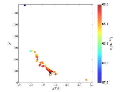
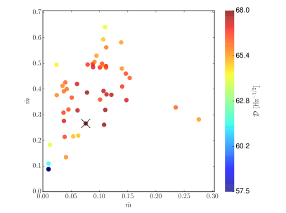
Data with gaps and noise floor fluctuations

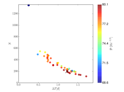
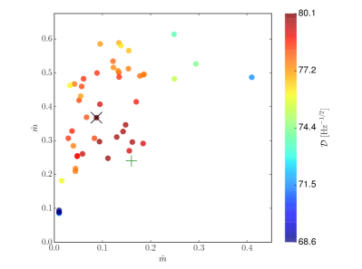
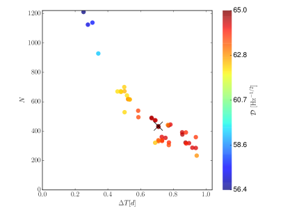
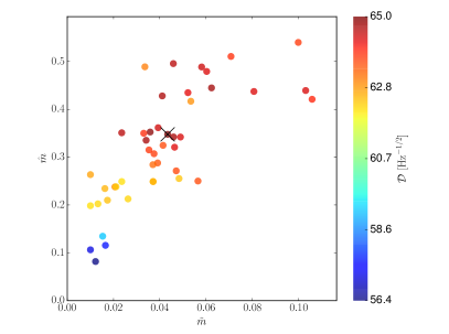
In this example we further relax the requirements on the data by allowing noise floor fluctuations, while keeping the duty cycle of $70\ \%$ per detector. For each SFT the PSD has been drawn from a Gaussian distribution with mean $E[\sqrt{S_{\mathrm{n}}}]=1\ \mathrm{Hz}^{-1/2}$ and standard deviation $\sigma[\sqrt{S_{\mathrm{n}}}]=15\times 10^{-2}\ \mathrm{Hz}^{-1/2}$. The outcome of the optimization is plotted in Fig. 4. The optimal parameters are summarized in Table 3.

	greedy	compact	greedy-compact
$\mathcal{D}\,[\mathrm{Hz}^{-1/2}]$	$64.8$	$68.0$	$64.8$
$T\,[\mathrm{d}]$	364.9	215.3	364.8
$N$	454.1	154.6	423
$\Delta T\,[\mathrm{d}]$	0.7	1.4	0.7
$\widetilde{m}$	0.03	0.08	0.04
$\widehat{m}$	0.32	0.27	0.35

Table 3: Optimal solution using greedy, compact and greedy-compact data selection applied to data from 2 detectors, with 70 % duty cycle and noise floor with fluctuations.

(a)

(b)

(c)

(d)

(e)

(f)

Figure 4: Semicoherent search optimization for data from 2 detectors with duty cycle 70% and noise floor with fluctuations. The cost constraint is $C_{0}=472.0\,\mathrm{d}$. The best numerical solution is denoted with $\times$. The panels on the left side show optimal segment duration $\Delta T$ and number of segments $N$, and the panels on the right side show optimal coherent $\widetilde{m}$ and semicoherent $\widehat{m}$ mismatch. Panels (a) and (b) are obtained using greedy data selection, the most sensitive optimal solution is ${\widetilde{m}}_{\mathrm{opt}}\approx 0.03$, ${\widehat{m}}_{\mathrm{opt}}\approx 0.32$, ${\Delta T}_{\mathrm{opt}}\approx 0.7\ \mathrm{d}$, ${N}_{\mathrm{opt}}\approx 454.1$, ${T}_{\mathrm{opt}}\approx 364.9\ \mathrm{d}$, $\widetilde{n}=2$, $\widehat{n}=3$, $\mathcal{D}\approx$64.6$\,\mathrm{Hz}^{-1/2}$ . Panels (c) and (d) are obtained using compact data selection, the most sensitive optimal solution is ${\widetilde{m}}_{\mathrm{opt}}\approx 0.08$, ${\widehat{m}}_{\mathrm{opt}}\approx 0.27$, ${\Delta T}_{\mathrm{opt}}\approx 1.4\ \mathrm{d}$, ${N}_{\mathrm{opt}}\approx 154.6$, ${T}_{\mathrm{opt}}\approx 215.3\ \mathrm{d}$, $\widetilde{n}=2$, $\widehat{n}=3$, $\mathcal{D}\approx$68.0$\,\mathrm{Hz}^{-1/2}$ . Panels (e) and (f) are obtained using greedy-compact data selection, the most sensitive optimal solution is ${\widetilde{m}}_{\mathrm{opt}}\approx 0.04$, ${\widehat{m}}_{\mathrm{opt}}\approx 0.35$, ${\Delta T}_{\mathrm{opt}}\approx 0.7\ \mathrm{d}$, ${N}_{\mathrm{opt}}\approx 423.0$, ${T}_{\mathrm{opt}}\approx 364.8\ \mathrm{d}$, $\widetilde{n}=2$, $\widehat{n}=3$, $\mathcal{D}\approx$64.8$\,\mathrm{Hz}^{-1/2}$

IV.2 Directed search using real data

In this subsection we apply the optimization procedure to real data collected by the Hanford (H1) and Livingston (L1) LIGO detectors during the S5 run Abbott et al. (2009a). The most sensitive data is found around $169.875\ \mathrm{Hz}$, thus the optimization will be done at this frequency. The details about the data are summarized in Table 4. It spans 653 days in 17797 SFTs of duration $T_{\mathrm{SFT}}=1800\ \mathrm{s}$. With this the average duty cycle is approximately $0.28$ in each detector.

run	detector	$f$ [Hz]	first SFT	last SFT	$N_{\mathrm{SFT}}$	$T_{\mathrm{span}}$ [d]
S5	H1	169.875	818845553	875277921	9331	653
S5	L1	169.875	818845553	875278812	8466	653

Table 4: Detector data used to test the numerical optimization under real conditions.

Keeping the cost constraint

We first keep the cost constraint equal to the computing cost used in the examples with simulated data, namely $C_{0}\approx 472$ days. The result of the optimization procedure is plotted in Fig. 5. We summarize the optimal parameters in Table 5. In this case usage of the compact data selection algorithm yields approximately 10% increase of the search depth compared to the other two methods. The gain of search depth compared to the fully-coherent solution is approximately $1.5\$.

	greedy	compact	greedy-compact
$\mathcal{D}\,[\mathrm{Hz}^{-1/2}]$	$56.9$	$63.4$	$56.5$
$T\,[\mathrm{d}]$	554.4	329.0	653.0
$N$	182.2	134.3	183.1
$\Delta T\,[\mathrm{d}]$	0.9	1.0	0.8
$\widetilde{m}$	0.06	0.05	0.04
$\widehat{m}$	0.61	0.27	0.55

Table 5: Optimal solution using greedy, compact and greedy-compact data selection applied to data from the H1 and L1 LIGO detectors during the S5 run.

(a)

(b)

(c)

(d)

(e)

(f)

Figure 5: Semicoherent search optimization for data from the H1 and L1 LIGO detectors during the S5 run at $169.875\ \mathrm{Hz}$. The cost constraint is $C_{0}=472.0\ \mathrm{d}$. The best numerical solution is denoted with $\times$. The panels on the left side show optimal segment duration $\Delta T$ and number of segments $N$, and the panels on the right side show optimal coherent $\widetilde{m}$ and semicoherent $\widehat{m}$ mismatch. Panels (a) and (b) are obtained using greedy data selection, the most sensitive optimal solution is ${\widetilde{m}}_{\mathrm{opt}}\approx 0.06$, ${\widehat{m}}_{\mathrm{opt}}\approx 0.61$, ${\Delta T}_{\mathrm{opt}}\approx 0.9\ \mathrm{d}$, ${N}_{\mathrm{opt}}\approx 182.2$, ${T}_{\mathrm{opt}}\approx 554.4\ \mathrm{d}$, $\widetilde{n}=2$, $\widehat{n}=3$, $\mathcal{D}\approx$56.9$\,\mathrm{Hz}^{-1/2}$ . Panels (c) and (d) are obtained using compact data selection, the most sensitive optimal solution is ${\widetilde{m}}_{\mathrm{opt}}\approx 0.05$, ${\widehat{m}}_{\mathrm{opt}}\approx 0.27$, ${\Delta T}_{\mathrm{opt}}\approx 1.0\ \mathrm{d}$, ${N}_{\mathrm{opt}}\approx 134.3$, ${T}_{\mathrm{opt}}\approx 329.0\ \mathrm{d}$, $\widetilde{n}=2$, $\widehat{n}=3$, $\mathcal{D}\approx$63.4$\,\mathrm{Hz}^{-1/2}$ . Panels (e) and (f) are obtained using greedy-compact data selection, the most sensitive optimal solution is ${\widetilde{m}}_{\mathrm{opt}}\approx 0.04$, ${\widehat{m}}_{\mathrm{opt}}\approx 0.55$, ${\Delta T}_{\mathrm{opt}}\approx 0.8\ \mathrm{d}$, ${N}_{\mathrm{opt}}\approx 183.1$, ${T}_{\mathrm{opt}}\approx 653.0\ \mathrm{d}$, $\widetilde{n}=2$, $\widehat{n}=3$, $\mathcal{D}\approx$56.5$\,\mathrm{Hz}^{-1/2}$

Using Einstein@Home

Finally we consider using the Einstein@Home distributed computing environment to increase the computing cost constraint to $C_{0}=360\times 10^{3}$ days on a single computing core. Such computing power corresponds to approximately 30 days on 12000 24x7 single core CPUs.

	greedy	compact	greedy-compact
$\mathcal{D}\,[\mathrm{Hz}^{-1/2}]$	$98.6$	$97.9$	$95.6$
$T\,[\mathrm{d}]$	464.8	387.7	653.2
$N$	20	20	35.2
$\Delta T\,[\mathrm{d}]$	15.4	17.9	9.8
$\widetilde{m}$	0.10	0.11	0.04
$\widehat{m}$	0.28	0.29	0.26

Table 6: Optimal solution using greedy, compact and greedy-compact data selection applied to data from the H1 and L1 LIGO detectors during the S5 run. The cost constraint is suitable with Einstein@Home.

(a)

(b)

(c)

(d)

(e)

(f)

Figure 6: Semicoherent search optimization with data from the H1 and L1 LIGO detectors during the S5 run at $169.875\ \mathrm{Hz}$. The cost constraint is $C_{0}=360\times 10^{3}\ \mathrm{d}$. The best numerical solution is denoted with $\times$. The panels on the left side show optimal segment duration $\Delta T$ and number of segments $N$, and the panels on the right side show optimal coherent $\widetilde{m}$ and semicoherent $\widehat{m}$ mismatch. Panels (a) and (b) are obtained using greedy data selection, the most sensitive optimal solution is ${\widetilde{m}}_{\mathrm{opt}}\approx 0.10$, ${\widehat{m}}_{\mathrm{opt}}\approx 0.28$, ${\Delta T}_{\mathrm{opt}}\approx 15.4\ \mathrm{d}$, ${N}_{\mathrm{opt}}\approx 20.0$, ${T}_{\mathrm{opt}}\approx 464.8\ \mathrm{d}$, $\widetilde{n}=2$, $\widehat{n}=3$, $\mathcal{D}\approx$98.6$\,\mathrm{Hz}^{-1/2}$ . Panels (c) and (d) are obtained using compact data selection, the most sensitive optimal solution is ${\widetilde{m}}_{\mathrm{opt}}\approx 0.11$, ${\widehat{m}}_{\mathrm{opt}}\approx 0.29$, ${\Delta T}_{\mathrm{opt}}\approx 17.9\ \mathrm{d}$, ${N}_{\mathrm{opt}}\approx 20.0$, ${T}_{\mathrm{opt}}\approx 387.7\ \mathrm{d}$, $\widetilde{n}=3$, $\widehat{n}=3$, $\mathcal{D}\approx$97.9$\,\mathrm{Hz}^{-1/2}$ . Panels (e) and (f) are obtained using greedy-compact data selection, the most sensitive optimal solution is ${\widetilde{m}}_{\mathrm{opt}}\approx 0.04$, ${\widehat{m}}_{\mathrm{opt}}\approx 0.26$, ${\Delta T}_{\mathrm{opt}}\approx 9.8\ \mathrm{d}$, ${N}_{\mathrm{opt}}\approx 35.2$, ${T}_{\mathrm{opt}}\approx 653.2\ \mathrm{d}$, $\widetilde{n}=2$, $\widehat{n}=3$, $\mathcal{D}\approx$95.6$\,\mathrm{Hz}^{-1/2}$

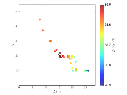
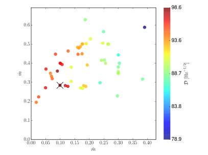
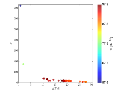
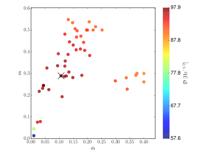
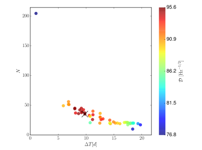
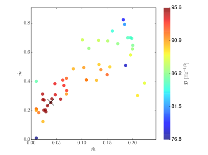
The results of the numerical optimization procedure approximation are plotted in Fig. 6. The optimal parameters are given in Table 6.

Note, that by the enormous increase of the computing power, the three different data selection methods yield practically equal sensitivity and the gain in sensitivity compared to the fully coherent solution is approximately $2.65\$.

V Discussion

In this paper we studied the optimization of semicoherent searches for continuous gravitational waves, in particular the StackSlide search, at constrained computing cost under more realistic conditions by taking into account possible gaps in the data and noise level changes. The presented method to obtain optimal search parameters is based on numerical optimization combined with a data selection algorithm. The outcome of the optimization procedure is the set of the optimal search parameters $\{\widetilde{m}\ ,\widehat{m},N,\ \Delta T\}$ as well as the selected data and an estimate of the expected sensitivity depth.

We showed that under ideal conditions, our numerical optimization method recovers, in terms of sensitivity, the optimal solution found by using the analytical method discussed in Ref. Prix and Shaltev (2012). Based on the examples of practical application, we conclude that the compact data selection yields higher sensitivity depth compared to the greedy data selection. However the superiority of the compact method over the greedy method depends on the data quality and on the computing cost constraint. It diminishes namely for data without large differences in the noise level from epoch to epoch and equally distributed gaps or for large allowed computing cost, where we can use nearly all the data.

The optimization procedure is immediately applicable to searches over simple (nearly) ”box“ parameter-space shape. While the proposed optimization method can be easily adapted to other types of searches, by modification of the computing cost function, further work is required to extend the applicability of the optimization procedure to an arbitrary parameter-space shape. The proposed optimization method assumed a fixed frequency band. Further work is required to relax this condition, in order to answer the question, what is the optimal trade-off between the size of the searched parameter space (width of the search) and its coverage (depth of the search). For a promising approach see Ming et al. (2015). In the example section of this paper we considered directed searches. For further work on all-sky searches one should take into account recent research on the semicoherent metric Wette (2015), as it suggests increase of the semicoherent number of templates with yet unknown implications.

VI Acknowledgments

MS would like to acknowledge the numerous comments and suggestions of Reinhard Prix. The author is also thankful for the discussions with Karl Wette, Badri Krishnan, Sinead Walsh and Maria Alessandra Papa. MS gratefully acknowledges the support of Bruce Allen and the IMPRS on Gravitational Wave Astronomy of the Max-Planck-Society. The numerical optimizations in this work have been performed on the ATLAS computing cluster of the Max-Planck-Institut für Gravitationsphysik. This paper has been assigned LIGO document number LIGO-P1500178-v3.

Appendix A Pseudo code of the proposed data selection algorithms

In the following we describe the data selection algorithms proposed in Sec. III in pseudo code.

List of Algorithms 1 Greedy data selection.

Input $\mathcal{D}$ - list of SFTs sorted by increasing timestamp $t_{j}$, $N$ - requested number of segments with duration $\Delta T$

Output $\mathcal{L}$ - list of segments and corresponding SFTs

while Length($\mathcal{L}$)$<N$ && Length($\mathcal{D}$) $>0$ do

     $\mathcal{G}\leftarrow 0$$\triangleright$ List of goodness per segment

     for all $t_{j}$ do

         $d\leftarrow$FindAllSFTsInRange($t_{j},t_{j}+\Delta T$)

         $\mathcal{G}_{j}\leftarrow$ComputeGoodness(d)

     end for

     $g\leftarrow$Max($\mathcal{G}$)

     $\mathcal{L}_{j}\leftarrow$AddSegment(g)

     RemoveUsedSFTs($\mathcal{L}_{j}$)

end while

List of Algorithms 2 Compact data selection.

Input $\mathcal{D}$ - list of SFTs sorted by increasing timestamp $t_{j}$, $N$ - requested number of segments with duration $\Delta T$

Output $\mathcal{L}$ - list of segments and corresponding SFTs

$\mathcal{G}\leftarrow 0$$\triangleright$ List of goodness

$L\leftarrow 0$$\triangleright$ List of segmentlists

for all $t_{j}$ do

     $t_{s}\leftarrow t_{j}$

     $l\leftarrow 0$

     while Length($l$)$<N$ && $t_{s}<$Max($t_{j}$) do

         $d\leftarrow$FindAllSFTsInRange($t_{s},t_{s}+\Delta T$)

         $l_{j}\leftarrow$AddSegment(d)

         $t_{s}\leftarrow$FirstTimestampAfter($t_{s}+\Delta T$)

     end while

     $L_{j}\leftarrow l$

     $\mathcal{G}_{j}\leftarrow$ComputeGoodness($L_{j}$)

end for

$\mathcal{L}\leftarrow$Max($\mathcal{G}$)$\triangleright$ such that the computing cost constraint is satisfied

List of Algorithms 3 Greedy-compact data selection.

Input $\mathcal{D}$ - list of SFTs sorted by increasing timestamp $t_{j}$, $N$ - requested number of segments with duration $\Delta T$

Output $\mathcal{L}$ - list of segments and corresponding SFTs

while Length($\mathcal{L}$)$<N$ && Length($\mathcal{D}$) $>0$ do

     $\mathcal{X}\leftarrow 0$$\triangleright$ List of goodness / cost ratio

     for all $t_{j}$ do

         $d\leftarrow$FindAllSFTsInRange($t_{j},t_{j}+\Delta T$)

         $\mathcal{X}_{j}\leftarrow$ComputeGoodnessCostRatio(d)

     end for

     $x\leftarrow$Max($\mathcal{X}$)

     $\mathcal{L}_{j}\leftarrow$AddSegment($x$)

     RemoveUsedSFTs($\mathcal{L}_{j}$)

end while

References

- Prix and Shaltev (2012) R. Prix and M. Shaltev, Phys. Rev. D 85, 084010 (2012), URL http://link.aps.org/doi/10.1103/PhysRevD.85.084010.
- Jaranowski et al. (1998a) P. Jaranowski, A. Krolak, and B. F. Schutz, Phys. Rev. D58, 063001 (1998a), eprint gr-qc/9804014.
- Brady and Creighton (2000) P. R. Brady and T. Creighton, Phys. Rev. D61, 082001 (2000), eprint gr-qc/9812014.
- Cutler et al. (2005) C. Cutler, I. Gholami, and B. Krishnan, Phys. Rev. D 72, 042004 (2005).
- Ming et al. (2015) J. Ming, B. Krishnan, M. A. Papa, C. Aulbert, and H. Fehrmann (2015), eprint 1510.03417.
- Abbott et al. (2009a) B. P. Abbott et al. (LIGO Scientific), Rept. Prog. Phys. 72, 076901 (2009a), eprint 0711.3041.
- Aasi et al. (2015a) J. Aasi et al. (VIRGO, LIGO Scientific), Class. Quant. Grav. 32, 115012 (2015a), eprint 1410.7764.
- Wette (2012) K. Wette, Phys. Rev. D 85, 042003 (2012), URL http://link.aps.org/doi/10.1103/PhysRevD.85.042003.
- Abadie et al. (2010a) J. Abadie et al. (LIGO Scientific), Nucl. Instrum. Meth. A624, 223 (2010a), eprint 1007.3973.
- Prix and Wette (2012) R. Prix and K. Wette, LIGO DCC T1200272 (2012), eprint LIGO-T1200272, URL https://dcc.ligo.org/cgi-bin/private/DocDB/ShowDocument?docid=92001.
- Jaranowski et al. (1998b) P. Jaranowski, A. Królak, and B. F. Schutz, Phys. Rev. D 58, 063001 (1998b).
- Cutler and Schutz (2005) C. Cutler and B. F. Schutz, Phys. Rev. D 72, 063006 (2005).
- Prix (2007) R. Prix, Class. Quant. Grav. 24, S481 (2007).
- Pletsch (2010) H. J. Pletsch, Phys. Rev. D 82, 042002 (2010), eprint 1005.0395.
- Wette et al. (2008) K. Wette et al., Class. Quant. Grav. 25, 235011 (2008).
- Abadie et al. (2010b) J. Abadie et al. (LIGO Scientific Collaboration), Astrophys. J. 722, 1504 (2010b).
- Behnke et al. (2015) B. Behnke, M. A. Papa, and R. Prix, Phys. Rev. D 91, 064007 (2015), eprint 1410.5997.
- EAH (2015) Einstein@home, http://www.einsteinathome.org (2015).
- Abbott et al. (2008) B. Abbott et al. (LIGO Scientific Collaboration), Phys. Rev. D 77, 022001 (2008).
- Abbott et al. (2009b) B. Abbott et al. (LIGO Scientific Collaboration), Phys. Rev. D 80, 042003 (2009b).
- Aasi et al. (2013a) J. Aasi et al. (The LIGO Scientific Collaboration and the Virgo Collaboration), Phys. Rev. D 87, 042001 (2013a).
- Abbott et al. (2010) B. Abbott et al. (LIGO Scientific Collaboration and Virgo Collaboration), Astrophys. J. 713, 671 (2010).
- Aasi et al. (2013b) J. Aasi et al. (VIRGO, LIGO Scientific), Phys. Rev. D88, 102002 (2013b), eprint 1309.6221.
- Aasi et al. (2015b) J. Aasi et al. (LIGO), Astrophys. J. 813, 39 (2015b), eprint 1412.5942.
- Aasi et al. (2015c) J. Aasi et al. (LIGO Scientific), Class. Quant. Grav. 32, 074001 (2015c), eprint 1411.4547.
- Palomba (2005) C. Palomba, Mon. Not. Roy. Astron. Soc. 359, 1150 (2005), eprint astro-ph/0503046.
- Knispel and Allen (2008) B. Knispel and B. Allen, Phys. Rev. D78, 044031 (2008), eprint 0804.3075.
- Wade et al. (2012) L. Wade, X. Siemens, D. L. Kaplan, B. Knispel, and B. Allen, Phys. Rev. D86, 124011 (2012), eprint 1209.2971.
- Le Digabel (2011) S. Le Digabel, ACM Trans. Math. Softw. 37, 44:1 (2011), ISSN 0098-3500, URL http://doi.acm.org/10.1145/1916461.1916468.
- Audet and E (2004) C. Audet and J. E, SIAM Journal on optimization 17, 2006 (2004).
- Abramson et al. (2009) M. A. Abramson, C. Audet, J. E. Dennis, and S. L. Digabel, SIAM Journal on Optimization 20, 948 (2009), URL http://dblp.uni-trier.de/db/journals/siamjo/siamjo20.html#AbramsonADD09.
- Conn and Digabel (2011) A. R. Conn and S. L. Digabel, Optimization methods and software (2011).
- Wette (2015) K. Wette, Phys. Rev. D 92, 082003 (2015), URL http://link.aps.org/doi/10.1103/PhysRevD.92.082003.