Distributions of traces of Frobenius
for smooth plane curves over finite fields

Reynald Lercier DGA MI, La Roche Marguerite, 35174 Bruz, France. Institut de recherche mathématique de Rennes, Université de Rennes 1, Campus de Beaulieu, 35042 Rennes, France. reynald.lercier@m4x.org Christophe Ritzenthaler Institut de recherche mathématique de Rennes, Université de Rennes 1, Campus de Beaulieu, 35042 Rennes, France. christophe.ritzenthaler@univ-rennes1.fr Florent Rovetta Institut de Mathématiques de Luminy, UMR 6206 du CNRS, Luminy, Case 907, 13288 Marseille, France. florent.rovetta@univ-amu.fr Jeroen Sijsling Department of Mathematics, 27 N. Main Street, 6188 Kemeny Hall, Hanover, NH 03755-3551, United States of America. sijsling@gmail.com  and  Benjamin Smith INRIA, Laboratoire d’Informatique de l’École polytechnique (LIX), 91128 Palaiseau, France. smith@lix.polytechnique.fr
Abstract.

In a previous article, we obtained data on the distribution of traces of Frobenius of non-hyperelliptic genus 333 curves over small finite fields. In the present one, we give a heuristic explanation of these data, by extrapolating from results on the distribution of traces of Frobenius for plane curves whose degree is small with respect to the cardinality of their finite base field. In particular, our methods shed some new light on the asymmetry of the distribution around its mean value, which is related to the Serre obstruction.

Key words and phrases:
Genus 333 curves; plane quartics; moduli; families; enumeration; finite fields
2010 Mathematics Subject Classification:
14Q05; 14H10; 14H25; 14H37; 14H45; 14H50
The authors acknowledge support by grant ANR-09-BLAN-0020-01.

1. Introduction

More than 30 years ago, Serre found closed formulæ for the maximal possible number of rational points on a curve of genus g2𝑔2g\leq 2 over a finite field 𝔽qsubscript𝔽𝑞\mathbb{F}_{q}. The same article [28] also considered the problem of obtaining a similar formula for curves of genus 333. This problem is more involved, as Serre indeed noted at the time. The main obstruction to obtaining a closed formula is now known as the Serre obstruction: a principally polarized abelian threefold over 𝔽qsubscript𝔽𝑞\mathbb{F}_{q} that becomes the Jacobian of a genus 333 curve after base extension to 𝔽¯qsubscript¯𝔽𝑞\overline{\mathbb{F}}_{q} need not be the Jacobian of such a curve over 𝔽qsubscript𝔽𝑞\mathbb{F}_{q}. There is no such obstruction in dimension 1, because elliptic curves are their own Jacobians; nor in dimension 2, because all genus 222 curves are hyperelliptic (and thus their automorphism groups are isomorphic to those of their Jacobians, which which implies in general that such a descent is possible). The Serre obstruction appears in dimension 333 precisely because of the existence of non-hyperelliptic curves of genus 333.

There have been many computational and conceptual approaches to the Serre obstruction. Partial results can be found in [13, 19, 22, 23, 24, 27], while data for small fields can be found at manypoints.org. More general approaches were considered in [2, 17, 18]. However, so far none of these results can be used to give a closed formula in the sense of [28].

More precisely, the issue is as follows. The number of rational points on a given curve C𝐶C of genus g𝑔g over a finite field 𝔽qsubscript𝔽𝑞\mathbb{F}_{q} is given by

#C(𝔽q)=q+1t.#𝐶subscript𝔽𝑞𝑞1𝑡\#C(\mathbb{F}_{q})=q+1-t\ .

Here t𝑡t is the trace of Frobenius acting on the first étale cohomology group H1(Jét,)superscript𝐻1subscript𝐽étsubscriptH^{1}(J_{\text{\'{e}t}},\mathbb{Z}_{\ell}) of the Jacobian J𝐽J of C𝐶C, with \ell some prime not equal to p𝑝p. The classical Hasse–Weil–Serre bound shows that the absolute value of t𝑡t is bounded by 2gq2𝑔𝑞2g\sqrt{q}. The usual strategy for constructing maximal curves is to construct a principally polarized abelian variety A𝐴A over 𝔽qsubscript𝔽𝑞\mathbb{F}_{q} with a trace t𝑡t close to 2gq2𝑔𝑞-2g\sqrt{q}, so as to obtain a number of rational points that is close to the upper bound q+1+2gq𝑞12𝑔𝑞q+1+2g\sqrt{q}.

The Serre obstruction amounts to the fact that A𝐴A is not necessarily the Jacobian of a curve C𝐶C over 𝔽qsubscript𝔽𝑞\mathbb{F}_{q}. If it is not, then the quadratic twist of A𝐴A will be a Jacobian instead. However, taking such a quadratic twist changes the trace of Frobenius t𝑡t to t𝑡-t, so that the resulting C𝐶C has few points instead of many points.

This article was motivated by the hope of finding a new inroad to the problem, not by studying all descent problems for individual abelian varieties, but rather by an indirect approach: namely, by proving that for large negative values of t𝑡t there are more curves with trace t𝑡t than with trace t𝑡-t. More precisely, let 𝒩q,3(t)subscript𝒩𝑞3𝑡\mathcal{N}_{q,3}(t) be the number of non-hyperelliptic genus 333 curves over 𝔽qsubscript𝔽𝑞\mathbb{F}_{q} of trace t𝑡t up to 𝔽qsubscript𝔽𝑞\mathbb{F}_{q}-isomorphism. We are interested in studying the difference

𝒱q,3(t):=𝒩q,3(t)𝒩q,3(t)assignsubscript𝒱𝑞3𝑡subscript𝒩𝑞3𝑡subscript𝒩𝑞3𝑡\mathcal{V}_{q,3}(t):=\mathcal{N}_{q,3}(t)-\mathcal{N}_{q,3}(-t)

for 0t6q0𝑡6𝑞0\leq t\leq 6\sqrt{q}, and more specifically in proving that 𝒱q,3(t)0subscript𝒱𝑞3𝑡0\mathcal{V}_{q,3}(t)\leq 0 for large enough t𝑡t. This would be enough to show (using [19]) that there always exists a curve C𝐶C such that #C(𝔽q)q+1+32q3#𝐶subscript𝔽𝑞𝑞132𝑞3\#C(\mathbb{F}_{q})\geq q+1+3\lfloor 2\sqrt{q}\rfloor-3, and would moreover allow us to give the precise maximal value (see [26, Prop.4.1.7]).

A numerical study of 𝒱q,3(t)subscript𝒱𝑞3𝑡\mathcal{V}_{q,3}(t) for prime fields 𝔽qsubscript𝔽𝑞\mathbb{F}_{q} with 11q5311𝑞5311\leq q\leq 53 appears in [20]. Over these small fields, it was possible to construct all smooth non-hyperelliptic curves of genus 333 (that is, all smooth plane quartics) up to 𝔽qsubscript𝔽𝑞\mathbb{F}_{q}-isomorphism, and to compute the trace of a representative of each 𝔽qsubscript𝔽𝑞\mathbb{F}_{q}-isomorphism class. The resulting functions 𝒱q,3(t)subscript𝒱𝑞3𝑡\mathcal{V}_{q,3}(t) had some remarkable properties: for example, it always appeared that 𝒱q,3(t)subscript𝒱𝑞3𝑡\mathcal{V}_{q,3}(t) was negative for t>1.7q𝑡1.7𝑞t>1.7\sqrt{q}, so that the corresponding number of curves with many points was larger than the number of curves with few points. Our original hope that 𝒱q,3(t)subscript𝒱𝑞3𝑡\mathcal{V}_{q,3}(t) would always be negative for large enough t𝑡t turned out to be false in general, as was noted in [20]. Nevertheless, for each q𝑞q the data obtained fitted simple and pleasing graphs, and moreover these graphs almost coincided after normalizing by an explicit power of q𝑞q.

This phenomenon seemed interesting enough to merit further investigation. Moreover, it fits into a larger framework of results on the distribution of the number of rational points on curves over finite fields, as studied in [6, 7, 8, 9, 10, 16, 21, 33, 34] and especially [5]. The results of Bucur–David–Feigon–Lalín in [5] show that the number of rational points on plane curves of degree d𝑑d over 𝔽qsubscript𝔽𝑞\mathbb{F}_{q} is distributed according to an explicit and intuitive binomial law as long as d𝑑d is large enough compared to q𝑞q. We study this binomial law, or rather the normalized variation of this law around its mean, in Section 2. By the central limit theorem, this variation converges to 00; however, we show that after multiplying by a factor of q𝑞\sqrt{q}, its behavior as q𝑞q tends to infinity can be approximated by the function

ψ:x132πx(3x2)ex2/2.:𝜓maps-to𝑥132𝜋𝑥3superscript𝑥2superscript𝑒superscript𝑥22\psi:x\mapsto\frac{1}{3\sqrt{2\pi}}x(3-x^{2})e^{-x^{2}/2}\ .

In Section 3, using [5], we study the variation around the mean of the distribution of the number of rational points on plane curves of degree d𝑑d over 𝔽qsubscript𝔽𝑞\mathbb{F}_{q} as q𝑞q\to\infty for both general curves (Corollary 3.4) and smooth curves (Corollary 3.6). Along the way, we show by elementary methods that the bound dq2+q𝑑superscript𝑞2𝑞d\geq q^{2}+q of [5, Prop. 1.6] can be improved to d2q1𝑑2𝑞1d\geq 2q-1 (in Proposition 3.3). We note that in these cases, where d𝑑d is large compared to q𝑞q, the fact that there are more curves with large negative trace t𝑡t than with trace t𝑡-t is easy to see, since a curve with a large positive trace would have a negative number of rational points.

In Section 4, in contrast to the approach for sufficiently large d𝑑d above, we instead fix the particular small value d=4𝑑4d=4, while still letting q𝑞q tend to \infty. Here it remains a challenge to prove any exact results, but the comparison with our experiments in [20] is impressive. It would be especially interesting to see whether the observed phenomena persist for larger q𝑞q than those considered in these experiments. Our results are also consistent with those of [1], where it is conjectured that the distribution of the fraction of curves of genus g𝑔g over a fixed finite field 𝔽qsubscript𝔽𝑞\mathbb{F}_{q} whose number of points equals n𝑛n tends to a Poisson distribution as g𝑔g tends to infinity. More precisely, it is suggested as one runs over a set of curves over 𝔽qsubscript𝔽𝑞\mathbb{F}_{q} that represent the 𝔽qsubscript𝔽𝑞\mathbb{F}_{q}-rational points of the moduli stack of curves 𝖬gsubscript𝖬𝑔\mathsf{M}_{g}, one should have the following limit behavior:

limg#{C𝖬g(𝐅q):#C(𝔽q)=n}=λneλn!where λ=q+1+1q1 .subscript𝑔#conditional-set𝐶subscript𝖬𝑔subscript𝐅𝑞#𝐶subscript𝔽𝑞𝑛superscript𝜆𝑛superscript𝑒𝜆𝑛where λ=q+1+1q1 .\lim_{g\to\infty}\#\left\{C\in\mathsf{M}_{g}(\mathbf{F}_{q}):\#C(\mathbb{F}_{q})=n\right\}=\frac{\lambda^{n}e^{-\lambda}}{n!}\quad\text{where $\lambda=q+1+\frac{1}{q-1}$\ .}

The same argument as in the proof of Proposition 2.2 shows that the variation around the mean gives rise to the same distribution that we obtain in our paper.

Acknowledgments

We are very grateful to Mohamed Barakat for his helpful comments, Masaaki Homma for his proof of Lemma 3.2, Everett Howe for email exchanges which led us to the heuristic interpretation described in this article, and Atilla Yilmaz for pointing out the link between our statistical result and Edgeworth series.

2. Some remarks on the binomial distribution

We begin by analyzing the asymmetry of the binomial distribution around its mean in a general context. We will then adapt the parameters according to our arithmetical problems.

Let us consider the the binomial random variable of standard deviation σ𝜎\sigma

Sσ:=i=1NσBσ,iassignsubscript𝑆𝜎superscriptsubscript𝑖1subscript𝑁𝜎subscript𝐵𝜎𝑖S_{\sigma}:=\sum_{i=1}^{N_{\sigma}}B_{\sigma,i}\

given by Nσsubscript𝑁𝜎N_{\sigma} Bernoulli random variables Bσ,isubscript𝐵𝜎𝑖B_{\sigma,i} taking the value 111 with probability μσsubscript𝜇𝜎\mu_{\sigma}. Let

bσ(m):=Prob(Sσ=m)=(Nσm)μσm(1μσ)(Nσm)assignsubscript𝑏𝜎𝑚Probsubscript𝑆𝜎𝑚binomialsubscript𝑁𝜎𝑚superscriptsubscript𝜇𝜎𝑚superscript1subscript𝜇𝜎subscript𝑁𝜎𝑚b_{\sigma}(m):=\operatorname{Prob}(S_{\sigma}=m)={N_{\sigma}\choose m}\mu_{\sigma}^{m}(1-\mu_{\sigma})^{(N_{\sigma}-m)}

be the corresponding binomial mass function of mean Eσ=Nσμσsubscript𝐸𝜎subscript𝑁𝜎subscript𝜇𝜎E_{\sigma}=N_{\sigma}\mu_{\sigma}. We have the usual relation

σ=Nσμσ(1μσ).𝜎subscript𝑁𝜎subscript𝜇𝜎1subscript𝜇𝜎\sigma=\sqrt{N_{\sigma}\mu_{\sigma}(1-\mu_{\sigma})}\ .

Let us now consider an increasing sequence of σ𝜎\sigma. For any fixed real α>0𝛼0\alpha>0, we define a sequence of intervals Iσ=[σ1α,σ1α]subscript𝐼𝜎superscript𝜎1𝛼superscript𝜎1𝛼I_{\sigma}=[-\sigma^{1-\alpha},\sigma^{1-\alpha}]. In order to deal with approximations in both σ𝜎\sigma and xIσ𝑥subscript𝐼𝜎x\in I_{\sigma}, we need one more piece of notation.

Definition 2.1.

Suppose that for all (sufficiently large) σ𝜎{\sigma} we are given an interval Iσsubscript𝐼𝜎I_{\sigma} along with functions fσsubscript𝑓𝜎f_{\sigma} and gσsubscript𝑔𝜎g_{\sigma} on Iσsubscript𝐼𝜎I_{\sigma}. We write fσ=o(gσ)subscript𝑓𝜎𝑜subscript𝑔𝜎f_{\sigma}=o(g_{\sigma}) if for all ϵ>0italic-ϵ0\epsilon>0, there exists a σ0subscript𝜎0{\sigma}_{0} such that

|fσ(x)|ϵ|gσ(x)|xIσ,σ>σ0.formulae-sequencesubscript𝑓𝜎𝑥italic-ϵsubscript𝑔𝜎𝑥formulae-sequencefor-all𝑥subscript𝐼𝜎for-all𝜎subscript𝜎0{|f_{\sigma}(x)|}\leq\epsilon|g_{\sigma}(x)|\quad\forall x\in I_{\sigma}\ ,\ \forall{\sigma}>{\sigma}_{0}\ .

The notation fσ=O(gσ)subscript𝑓𝜎𝑂subscript𝑔𝜎f_{\sigma}=O(g_{\sigma}) is defined similarly.

The triangular central limit theorem [4, Th.27.3] shows111 This can also be deduced from the De Moivre–Laplace theorem [4, Ex. 25.11], which claims that if (mσ)σsubscriptsubscript𝑚𝜎𝜎(m_{\sigma})_{\sigma} is any sequence of integers such that (mσEσ)/σsubscript𝑚𝜎subscript𝐸𝜎𝜎(m_{\sigma}-E_{\sigma})/\sigma tends to some real x𝑥x as σ𝜎{\sigma}\to\infty then limσσProb(Sσ=mσ)=12πe12x2subscript𝜎𝜎Probsubscript𝑆𝜎subscript𝑚𝜎12𝜋superscript𝑒12superscript𝑥2\lim_{{\sigma}\to\infty}\sigma\operatorname{Prob}(S_{{\sigma}}=m_{\sigma})=\frac{1}{\sqrt{2\pi}}e^{-\frac{1}{2}x^{2}}. that the normalized average sequence Yσ:=(SσEσ)/σassignsubscript𝑌𝜎subscript𝑆𝜎subscript𝐸𝜎𝜎Y_{{\sigma}}:=(S_{\sigma}-E_{\sigma})/\sigma converges in law to the standard normal distribution: that is, the cumulative distribution law of the random variable Yσsubscript𝑌𝜎Y_{{\sigma}} converges to the integral of the Gaussian density. We therefore see that Yσ(x)Yσ(x)subscript𝑌𝜎𝑥subscript𝑌𝜎𝑥Y_{\sigma}(x)-Y_{\sigma}(-x) tends to 00 as σ𝜎{\sigma}\to\infty.

In order to deal with asymptotic approximations (in σ𝜎\sigma) of Sσsubscript𝑆𝜎S_{\sigma}, we introduce a new continuous function that we will call b𝑏b. We define

m(σ,x)𝑚𝜎𝑥\displaystyle m({\sigma},x) :=Eσσx,assignabsentsubscript𝐸𝜎𝜎𝑥\displaystyle:=E_{\sigma}-\sigma x\ ,
n(σ,x)𝑛𝜎𝑥\displaystyle n({\sigma},x) :=Nσ(1μσ)+σx=Nσm(σ,x).assignabsentsubscript𝑁𝜎1subscript𝜇𝜎𝜎𝑥subscript𝑁𝜎𝑚𝜎𝑥\displaystyle:=N_{\sigma}(1-\mu_{\sigma})+\sigma x=N_{\sigma}-m({\sigma},x)\ .

Then if σ𝜎{\sigma} is large enough, we define the aforementioned continuous function b𝑏b by

b(σ,x):=Γ(Nσ+1)Γ(n(σ,x)+1)Γ(m(σ,x)+1)μσm(σ,x)(1μσ)n(σ,x).assign𝑏𝜎𝑥Γsubscript𝑁𝜎1Γ𝑛𝜎𝑥1Γ𝑚𝜎𝑥1superscriptsubscript𝜇𝜎𝑚𝜎𝑥superscript1subscript𝜇𝜎𝑛𝜎𝑥b({\sigma},x):=\frac{\Gamma(N_{\sigma}+1)}{\Gamma(n({\sigma},x)+1)\Gamma(m({\sigma},x)+1)}\mu_{\sigma}^{m({\sigma},x)}(1-\mu_{\sigma})^{n({\sigma},x)}\ . (2.1)

Observe that if m(σ,x)𝑚𝜎𝑥m({\sigma},x) happens to be integral, then

b(σ,x)=bσ(m(σ,x));𝑏𝜎𝑥subscript𝑏𝜎𝑚𝜎𝑥b({\sigma},x)=b_{\sigma}(m({\sigma},x))\ ;

as such, b(σ,x)𝑏𝜎𝑥b({\sigma},x) should be thought of as the collection of continuous interpolations of these values, with the difference that we have switched to using the normalized parameter x𝑥x instead of m𝑚m.

Proposition 2.2.

With the previous notation, assume that Eσ=σ2+1+O(1/σ2)subscript𝐸𝜎superscript𝜎21𝑂1superscript𝜎2E_{\sigma}=\sigma^{2}+1+O(1/\sigma^{2}) when σ𝜎\sigma tends to infinity, and let α>0𝛼0\alpha>0 be any fixed real. Then for x[σ1α,σ1α]𝑥superscript𝜎1𝛼superscript𝜎1𝛼x\in[-\sigma^{1-\alpha},\sigma^{1-\alpha}] , we have

b(σ,x)=(12πe12x2)1σ(162πx(x23)e12x2)1σ2+O(1σ3).𝑏𝜎𝑥12𝜋superscript𝑒12superscript𝑥21𝜎162𝜋𝑥superscript𝑥23superscript𝑒12superscript𝑥21superscript𝜎2𝑂1superscript𝜎3b(\sigma,x)=\left(\frac{1}{\sqrt{2\pi}}{e^{-\frac{1}{2}x^{2}}}\right)\frac{1}{\sigma}-\left(\frac{1}{6\sqrt{2\pi}}x(x^{2}-3)e^{-\frac{1}{2}x^{2}}\right)\frac{1}{\sigma^{2}}+O\left(\frac{1}{\sigma^{3}}\right)\ .

We defer the proof, which is long and technical, to Section 5.

Corollary 2.3.

With the notation of Proposition 2.2,

b(σ,x)b(σ,x)=(132πx(3x2)e12x2)1σ2+O(1σ3).𝑏𝜎𝑥𝑏𝜎𝑥132𝜋𝑥3superscript𝑥2superscript𝑒12superscript𝑥21superscript𝜎2𝑂1superscript𝜎3b(\sigma,x)-b(\sigma,-x)=\left(\frac{1}{3\sqrt{2\pi}}x(3-x^{2})e^{-\frac{1}{2}x^{2}}\right)\frac{1}{\sigma^{2}}+O\left(\frac{1}{\sigma^{3}}\right)\ .
Remark 2.4.

The error terms in the central limit theorem are well-studied, and there are powerful tools to deal with them in the literature. However, the usual Edgeworth series techniques do not seem to apply here. Indeed, while the expressions involved are identical (for example, the polynomial x(3x2)𝑥3superscript𝑥2x(3-x^{2}) appearing in Proposition 2.2 is the negative of the third Hermite polynomial [15, Sec. 3.4]), the interval Iσsubscript𝐼𝜎I_{\sigma} of convergence we obtain, which is optimal, is not the interval predicted by a formal application of Edgeworth series we found in the literature.
Refer to caption
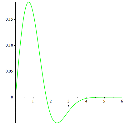
Figure 1. The graph of the approximation ψ:x132πx(x23)ex2/2:𝜓maps-to𝑥132𝜋𝑥superscript𝑥23superscript𝑒superscript𝑥22\psi:x\mapsto\frac{1}{3\sqrt{2\pi}}x(x^{2}-3)e^{-x^{2}/2}.

We will use these results in Sections 2 and 3 with the following parameters. We assume that the probabilities for a plane curve over 𝔽qsubscript𝔽𝑞\mathbb{F}_{q} to pass through any one of the q2+q+1superscript𝑞2𝑞1q^{2}+q+1 points of the projective plane are described by independent and identically distributed random variables with probability 1/q+O(1/q2)1𝑞𝑂1superscript𝑞21/q+O(1/q^{2}). More precisely, we will apply the results for the following values.

  1. (1)

    In Corollary 3.4 we will have σ=q1/q2=q+O(q5/2)𝜎𝑞1superscript𝑞2𝑞𝑂superscript𝑞52\sigma=\sqrt{q-1/q^{2}}=\sqrt{q}+O(q^{-5/2}), μσ=1/qsubscript𝜇𝜎1𝑞\mu_{\sigma}=1/q, and

    Eσ=(q2+q+1)/q=σ2+1+O(1/q)=σ2+1+O(1/σ2).subscript𝐸𝜎superscript𝑞2𝑞1𝑞superscript𝜎21𝑂1𝑞superscript𝜎21𝑂1superscript𝜎2E_{\sigma}=(q^{2}+q+1)/q=\sigma^{2}+1+O(1/q)=\sigma^{2}+1+O(1/\sigma^{2}).
  2. (2)

    In Corollary 3.6 we will have σ=q(11q2+q+1)𝜎𝑞11superscript𝑞2𝑞1\sigma=\sqrt{q(1-\frac{1}{q^{2}+q+1})}, μσ=(q+1)/(q2+q+1)subscript𝜇𝜎𝑞1superscript𝑞2𝑞1\mu_{\sigma}=(q+1)/(q^{2}+q+1), and

    Eσ=q+1=σ2+1+O(1/σ2).subscript𝐸𝜎𝑞1superscript𝜎21𝑂1superscript𝜎2E_{\sigma}=q+1=\sigma^{2}+1+O(1/\sigma^{2}).

In both situations, we meet the hypotheses of Proposition 2.2. Note that we can also apply our results to affine plane curves. Indeed, we pass through q2superscript𝑞2q^{2} points with probability μσ=1/qsubscript𝜇𝜎1𝑞\mu_{\sigma}=1/q so we have σ=q1𝜎𝑞1\sigma=\sqrt{q-1} and Eσ=σ2+1subscript𝐸𝜎superscript𝜎21E_{\sigma}=\sigma^{2}+1.

In the arithmetic setting below, the normalization will not be m(σ,x)=Eσσx𝑚𝜎𝑥subscript𝐸𝜎𝜎𝑥m(\sigma,x)=E_{\sigma}-\sigma x but q+1qx𝑞1𝑞𝑥q+1-\sqrt{q}x. Hence we need to check that we can transfer the perturbation on x𝑥x induced by this transformation into the O(1/σ3)𝑂1superscript𝜎3O(1/\sigma^{3}). Since the main term of the expansion in Corollary 2.3 is x(x23)e12x2/σ2𝑥superscript𝑥23superscript𝑒12superscript𝑥2superscript𝜎2x(x^{2}-3)e^{-\frac{1}{2}x^{2}}/{\sigma^{2}}, if we replace x𝑥x by (m(σ,x)(q+1))/q=x+O(1/σ)𝑚𝜎𝑥𝑞1𝑞𝑥𝑂1𝜎(m(\sigma,x)-(q+1))/\sqrt{q}=x+O(1/\sigma), then the result still holds. This is the case in our applications.

3. Relation with the number of points on plane curves over finite fields.

The relation between the considerations in the previous section and the distribution of traces of Frobenius of plane curves over finite fields was first described by Bucur–David–Feigon–Lalín [5]. Let 𝔽qsubscript𝔽𝑞\mathbb{F}_{q} be the finite field with q𝑞q elements, and let R=𝔽q[x,y,z]𝑅subscript𝔽𝑞𝑥𝑦𝑧R=\mathbb{F}_{q}[x,y,z] be the homogeneous coordinate ring of the projective plane 2superscript2\mathbb{P}^{2} over 𝔽qsubscript𝔽𝑞\mathbb{F}_{q}. For f𝑓f in R𝑅R, we let Cf2subscript𝐶𝑓superscript2C_{f}\subset\mathbb{P}^{2} be the plane curve defined by f=0𝑓0f=0. Intuitively, the probability that a given point P𝑃P in 2(𝔽q)superscript2subscript𝔽𝑞\mathbb{P}^{2}(\mathbb{F}_{q}) lies on Cfsubscript𝐶𝑓C_{f} should equal 1/q1𝑞1/q, since a priori the set of possible values for f𝑓f at P𝑃P has q𝑞q elements (and P𝑃P is on C𝐶C if and only if f(P)=0𝑓𝑃0f(P)=0). Supposing furthermore that the probabilities are independent as P𝑃P varies over 2(𝔽q)superscript2subscript𝔽𝑞\mathbb{P}^{2}(\mathbb{F}_{q}), we essentially find ourselves in the situation of Section 2.

More precisely, let RdRsubscript𝑅𝑑𝑅R_{d}\subset R be the subset of homogeneous polynomials of degree d𝑑d, and consider curves defined by polynomials in Rdsubscript𝑅𝑑R_{d}. Then the following seminal result from [5] shows that the intuition above is accurate as long as d𝑑d is large enough with respect to q𝑞q.

Proposition 3.1 ([5, Prop. 1.6]).

Let B1,,Bq2+q+1subscript𝐵1subscript𝐵superscript𝑞2𝑞1B_{1},\ldots,B_{q^{2}+q+1} be i.i.d. Bernoulli random variables that assume the value 111 with probability 1/q1𝑞1/q. If dq2+q𝑑superscript𝑞2𝑞d\geq q^{2}+q, then

#{fRd:#Cf(𝔽q)=n}#Rd=Prob(B1++Bq2+q+1=n).#conditional-set𝑓subscript𝑅𝑑#subscript𝐶𝑓subscript𝔽𝑞𝑛#subscript𝑅𝑑Probsubscript𝐵1subscript𝐵superscript𝑞2𝑞1𝑛\frac{\#\{f\in R_{d}:\#C_{f}(\mathbb{F}_{q})=n\}}{\#R_{d}}=\operatorname{Prob}(B_{1}+\ldots+B_{q^{2}+q+1}=n)\ .

The original proof of Proposition 3.1 is based on a general result of Poonen [25]. However, we will give another proof by elementary means, improving the bound on d𝑑d in the process.

We choose an enumeration P1,,Pq2+q+1subscript𝑃1subscript𝑃superscript𝑞2𝑞1P_{1},\ldots,P_{q^{2}+q+1} of the set 2(𝔽q)superscript2subscript𝔽𝑞\mathbb{P}^{2}(\mathbb{F}_{q}), which we in turn lift to 𝔽qsubscript𝔽𝑞\mathbb{F}_{q}-rational affine representatives P~1,,P~q2+q+1subscript~𝑃1subscript~𝑃superscript𝑞2𝑞1\tilde{P}_{1},\ldots,\tilde{P}_{q^{2}+q+1} in 𝔸3(𝔽q)superscript𝔸3subscript𝔽𝑞\mathbb{A}^{3}(\mathbb{F}_{q}). This allows us to define the linear map

L:Rd(𝔽q):𝐿subscript𝑅𝑑subscript𝔽𝑞\displaystyle L:R_{d}(\mathbb{F}_{q}) 𝔽qq2+q+1,absentsuperscriptsubscript𝔽𝑞superscript𝑞2𝑞1\displaystyle\longrightarrow\mathbb{F}_{q}^{q^{2}+q+1}\ ,
f𝑓\displaystyle f (f(P~1),,f(P~q2+q+1)).absent𝑓subscript~𝑃1𝑓subscript~𝑃superscript𝑞2𝑞1\displaystyle\longmapsto(f(\tilde{P}_{1}),\ldots,f(\tilde{P}_{q^{2}+q+1}))\ .

The forms in the kernel of L𝐿L define the plane curves that pass through all rational points of the projective plane; these are called plane filling curves. It is known that the kernel of L𝐿L is Rd(𝔽q)Jsubscript𝑅𝑑subscript𝔽𝑞𝐽R_{d}(\mathbb{F}_{q})\cap J, where J𝐽J is the ideal generated by xqyyqxsuperscript𝑥𝑞𝑦superscript𝑦𝑞𝑥x^{q}y-y^{q}x, yqzzqysuperscript𝑦𝑞𝑧superscript𝑧𝑞𝑦y^{q}z-z^{q}y and zqxxqzsuperscript𝑧𝑞𝑥superscript𝑥𝑞𝑧z^{q}x-x^{q}z (see [30, 31] and [11, Prop.2.1]).

Lemma 3.2.

For d2q1𝑑2𝑞1d\geq 2q-1 the map L𝐿L is surjective.

Proof.

This proof is due to Masaaki Homma (see also his forthcoming article [12]). For any d2q1𝑑2𝑞1d\geq 2q-1, the degree d𝑑d polynomial xd(2q2)(yq1xq1)(zq1xq1)superscript𝑥𝑑2𝑞2superscript𝑦𝑞1superscript𝑥𝑞1superscript𝑧𝑞1superscript𝑥𝑞1x^{d-(2q-2)}(y^{q-1}-x^{q-1})(z^{q-1}-x^{q-1}) in Rdsubscript𝑅𝑑R_{d} takes a non-zero value at (1:0:0):10:0(1:0:0), and 00 at every other point in 2(𝔽q)superscript2subscript𝔽𝑞\mathbb{P}^{2}(\mathbb{F}_{q}). Using the transitive action of PGL3(𝔽q)subscriptPGL3subscript𝔽𝑞\operatorname{PGL}_{3}(\mathbb{F}_{q}), we see that we can construct degree d𝑑d polynomials having the same properties for any rational point of the plane. Therefore the evaluation map L𝐿L is surjective. ∎

Proposition 3.3.

Proposition 3.1 holds for d2q1𝑑2𝑞1d\geq 2q-1.

Proof.

Lemma 3.2 shows that under the given hypothesis on d𝑑d we can always find a homogeneous polynomial with a prescribed zero set of cardinality n𝑛n and given non-zero values on the complement. Hence, the cardinality of the set of such polynomials is the order of the kernel of L𝐿L, and does not depend on the prescribed zero set. This implies that the proportion of polynomials with a zero set of cardinality n𝑛n follows a binomial distribution Prob(B1++Bq2+q+1=n)Probsubscript𝐵1subscript𝐵superscript𝑞2𝑞1𝑛\operatorname{Prob}(B_{1}+\ldots+B_{q^{2}+q+1}=n). ∎

For a (possibly singular) plane curve Cfsubscript𝐶𝑓C_{f}, we let t=q+1#Cf(𝔽q)𝑡𝑞1#subscript𝐶𝑓subscript𝔽𝑞t=q+1-\#C_{f}(\mathbb{F}_{q}), and we define the normalized trace x:=t/qassign𝑥𝑡𝑞x:=t/\sqrt{q} in analogy with Section 2. Note that x𝑥x is not bounded as q𝑞q\to\infty. Let

Nq,d(x):=q#{fRd:#Cf(𝔽q)=q+1qx}#Rd;assignsubscript𝑁𝑞𝑑𝑥𝑞#conditional-set𝑓subscript𝑅𝑑#subscript𝐶𝑓subscript𝔽𝑞𝑞1𝑞𝑥#subscript𝑅𝑑N_{q,d}(x):=\sqrt{q}\cdot\frac{\#\{f\in R_{d}:\#C_{f}(\mathbb{F}_{q})=q+1-\sqrt{q}x\}}{\#R_{d}}\ ;

we want to approximate the difference

Vq,d(x):=q(Nq,d(x)Nq,d(x))assignsubscript𝑉𝑞𝑑𝑥𝑞subscript𝑁𝑞𝑑𝑥subscript𝑁𝑞𝑑𝑥V_{q,d}(x):=\sqrt{q}\cdot(N_{q,d}(x)-N_{q,d}(-x))

(note the normalization factor q𝑞\sqrt{q} which appears once in Nq,d(x)subscript𝑁𝑞𝑑𝑥N_{q,d}(x) and once in Vq,dsubscript𝑉𝑞𝑑V_{q,d}).

Corollary 3.4.

For d2q1𝑑2𝑞1d\geq 2q-1, any α>0𝛼0\alpha>0, and x[(q)1α,(q)1α]𝑥superscript𝑞1𝛼superscript𝑞1𝛼x\in[-(\sqrt{q})^{1-\alpha},(\sqrt{q})^{1-\alpha}], we get the following approximation of Vq,d(x)subscript𝑉𝑞𝑑𝑥V_{q,d}(x) (in the sense of Definition 2.1):

Vq,d(x)=132πx(3x2)ex2/2+O(1q).subscript𝑉𝑞𝑑𝑥132𝜋𝑥3superscript𝑥2superscript𝑒superscript𝑥22𝑂1𝑞V_{q,d}(x)=\frac{1}{3\sqrt{2\pi}}x(3-x^{2})\cdot e^{-x^{2}/2}+O\left(\frac{1}{\sqrt{q}}\right)\ .
Proof.

This follows from Proposition 3.3 and Section 2. ∎

We now restrict our considerations to nonsingular curves. Let RdnsRdsuperscriptsubscript𝑅𝑑nssubscript𝑅𝑑R_{d}^{\textrm{ns}}\subset R_{d} be the subset of homogeneous polynomials corresponding to nonsingular plane curves. Since we have restricted to a further subset defined by the non-vanishing of the rather complicated discriminant form, the sieving process to get the distribution is correspondingly more involved, and no elementary method seems to apply. Instead we use another result in [5].

Theorem 3.5 ([5, Th.1.1]).

Let B1,,Bq2+q+1subscript𝐵1subscript𝐵superscript𝑞2𝑞1B_{1},\ldots,B_{q^{2}+q+1} be i.i.d. Bernoulli random variables taking the value 111 with probability (q+1)/(q2+q+1)𝑞1superscript𝑞2𝑞1(q+1)/(q^{2}+q+1). If 0nq2+q+10𝑛superscript𝑞2𝑞10\leq n\leq q^{2}+q+1, then

#{fRdns:#Cf(𝔽q)=n}#Rdns=#conditional-set𝑓superscriptsubscript𝑅𝑑ns#subscript𝐶𝑓subscript𝔽𝑞𝑛#superscriptsubscript𝑅𝑑nsabsent\displaystyle\frac{\#\{f\in R_{d}^{\textrm{ns}}:\#C_{f}(\mathbb{F}_{q})=n\}}{\#R_{d}^{\textrm{ns}}}={} Prob(B1++Bq2+q+1=n)Probsubscript𝐵1subscript𝐵superscript𝑞2𝑞1𝑛\displaystyle\operatorname{Prob}(B_{1}+\ldots+B_{q^{2}+q+1}=n)
×(1+O(qn(d1/3+(d1)2qmin(dp+1,d3)+dqd1p1))).absent1𝑂superscript𝑞𝑛superscript𝑑13superscript𝑑12superscript𝑞𝑑𝑝1𝑑3𝑑superscript𝑞𝑑1𝑝1\displaystyle{}\times\left(1+O\left(q^{n}\left(d^{-1/3}+(d-1)^{2}q^{-\min(\lfloor\frac{d}{p}\rfloor+1,\frac{d}{3})}+dq^{-\lfloor\frac{d-1}{p}\rfloor-1}\right)\right)\right)\ .

As before, we let

Nq,dns(x):=q#{fRdns:#Cf(𝔽q)=q+1qx}#Rdns;assignsubscriptsuperscript𝑁ns𝑞𝑑𝑥𝑞#conditional-set𝑓superscriptsubscript𝑅𝑑ns#subscript𝐶𝑓subscript𝔽𝑞𝑞1𝑞𝑥#superscriptsubscript𝑅𝑑nsN^{\textrm{ns}}_{q,d}(x):=\sqrt{q}\cdot\frac{\#\{f\in R_{d}^{\textrm{ns}}:\#C_{f}(\mathbb{F}_{q})=q+1-\sqrt{q}x\}}{\#R_{d}^{\textrm{ns}}}\ ;

we want to analyze the difference

Vq,dns(x):=q(Nq,dns(x)Nq,dns(x)).assignsubscriptsuperscript𝑉ns𝑞𝑑𝑥𝑞subscriptsuperscript𝑁ns𝑞𝑑𝑥subscriptsuperscript𝑁ns𝑞𝑑𝑥V^{\textrm{ns}}_{q,d}(x):=\sqrt{q}\cdot(N^{\textrm{ns}}_{q,d}(x)-N^{\textrm{ns}}_{q,d}(-x))\ .

Using our Lemma, we see that Theorem 3.5 implies in particular that the same asympotic formula from Corollary 3.4 holds for smooth curves, except that the lower bound on d𝑑d is now doubly exponential instead of linear in q𝑞q. More precisely, we have the following.

Corollary 3.6.

For dq3(q2+q+2)𝑑superscript𝑞3superscript𝑞2𝑞2d\geq q^{3\,(q^{2}+q+2)}, any α>0𝛼0\alpha>0 and x[(q)1α,(q)1α]𝑥superscript𝑞1𝛼superscript𝑞1𝛼x\in[-(\sqrt{q})^{1-\alpha},(\sqrt{q})^{1-\alpha}], we get the following approximation of Vq,dns(x)subscriptsuperscript𝑉ns𝑞𝑑𝑥V^{\textrm{ns}}_{q,d}(x) (in the sense of Definition 2.1):

Vq,dns(x)=132πx(3x2)ex2/2+O(1q).subscriptsuperscript𝑉ns𝑞𝑑𝑥132𝜋𝑥3superscript𝑥2superscript𝑒superscript𝑥22𝑂1𝑞V^{\textrm{ns}}_{q,d}(x)=\frac{1}{3\sqrt{2\pi}}x(3-x^{2})\cdot e^{-x^{2}/2}+O\left(\frac{1}{\sqrt{q}}\right)\ .
Proof.

When dq3(q2+q+2)𝑑superscript𝑞3superscript𝑞2𝑞2d\geq q^{3\,(q^{2}+q+2)} the O()𝑂O() term in Theorem 3.5 is O(q1/2)𝑂superscript𝑞12O(q^{-1/2}); so applying Theorem 3.5 and Section 2 yields the result. ∎

4. Experimental results and their limitations

We consider the special case d=4𝑑4d=4. The smooth plane quartic curves Cfsubscript𝐶𝑓C_{f} defined by fR4ns(𝔽q)𝑓superscriptsubscript𝑅4nssubscript𝔽𝑞f\in R_{4}^{\textrm{ns}}(\mathbb{F}_{q}) are precisely the non-hyperelliptic curves of genus 333 over 𝔽qsubscript𝔽𝑞\mathbb{F}_{q}. Since d𝑑d is now fixed, our previous results cannot be applied directly. However, as mentioned in the introduction, we wish to compare the statistical distributions obtained in this way with the experimental results obtained in [20].

In order to do so, let us recall the notation of [20]. Let 𝒩q,3(t)subscript𝒩𝑞3𝑡\mathcal{N}_{q,3}(t) denote the number of 𝔽qsubscript𝔽𝑞\mathbb{F}_{q}-isomorphism classes of non-hyperelliptic curves of genus 333 over 𝔽qsubscript𝔽𝑞\mathbb{F}_{q} of trace t𝑡t, weighted by the order of their 𝔽qsubscript𝔽𝑞\mathbb{F}_{q}-automorphism group:

𝒩q,3(t):={C/𝔽qn.h. genus 3curve with tracet}/1#Aut𝔽q(C).assignsubscript𝒩𝑞3𝑡subscript𝐶subscript𝔽𝑞n.h. genus 3curve with trace𝑡absentsimilar-to-or-equals1#subscriptAutsubscript𝔽𝑞𝐶\mathcal{N}_{q,3}(t):=\sum_{\left\{\begin{subarray}{c}C/\mathbb{F}_{q}\,\textrm{n.h.\ genus 3}\\ \textrm{curve with trace}\;t\end{subarray}\right\}/\simeq}\frac{1}{\#\operatorname{Aut}_{\mathbb{F}_{q}}(C)}. (4.1)

This is the most natural way to define 𝒩q,3(t)subscript𝒩𝑞3𝑡\mathcal{N}_{q,3}(t) (c.f. [3, 32]). In order to compare our results for different values of q𝑞q, we renormalize 𝒩q,3(t)subscript𝒩𝑞3𝑡\mathcal{N}_{q,3}(t) to

𝒩q,3KS(x):=qq6+1𝒩q,3(t) where t:=qx for x[6,6].assignsubscriptsuperscript𝒩KS𝑞3𝑥𝑞superscript𝑞61subscript𝒩𝑞3𝑡 where 𝑡assign𝑞𝑥 for 𝑥66\mathcal{N}^{\textrm{KS}}_{q,3}(x):=\frac{\sqrt{q}}{q^{6}+1}\mathcal{N}_{q,3}(t)\ \text{ where }t:=\lfloor\sqrt{q}x\rfloor\text{ for }x\in[-6,6].

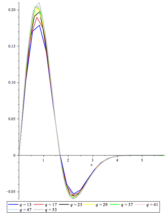
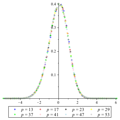
This coincides with the normalization of the trace distribution in Katz–Sarnak [14] (the factor q6+1superscript𝑞61q^{6}+1 being the number of 𝔽qsubscript𝔽𝑞\mathbb{F}_{q}-points of the moduli space of non hyperelliptic genus 333 curves). The numerical results in [20] on the quantity 𝒩q,3KS(x)subscriptsuperscript𝒩KS𝑞3𝑥\mathcal{N}^{\textrm{KS}}_{q,3}(x) and the difference

𝒱q,3KS(x):=q(𝒩q,3KS(x)𝒩q,3KS(x))assignsuperscriptsubscript𝒱𝑞3KS𝑥𝑞subscriptsuperscript𝒩KS𝑞3𝑥subscriptsuperscript𝒩KS𝑞3𝑥\mathcal{V}_{q,3}^{\textrm{KS}}(x):=\sqrt{q}\,(\mathcal{N}^{\textrm{KS}}_{q,3}(x)-\mathcal{N}^{\textrm{KS}}_{q,3}(-x))

are graphically summarized in Figure 2.
Refer to caption
(a) Graph of 𝒩q,3KS(x)subscriptsuperscript𝒩KS𝑞3𝑥\mathcal{N}^{\textrm{KS}}_{q,3}(x)
Refer to caption
(b) Linear interpolation of 𝒱q,3KS(x)superscriptsubscript𝒱𝑞3KS𝑥\mathcal{V}_{q,3}^{\textrm{KS}}(x)
Figure 2. The numerical trace distributions 𝒩q,3KS(x)subscriptsuperscript𝒩KS𝑞3𝑥\mathcal{N}^{\textrm{KS}}_{q,3}(x) and 𝒱q,3KS(x)subscriptsuperscript𝒱KS𝑞3𝑥\mathcal{V}^{\textrm{KS}}_{q,3}(x).

In order to apply our previous results, we need to understand the connection between Nq,4ns(x)superscriptsubscript𝑁𝑞4ns𝑥N_{q,4}^{\textrm{ns}}(x) and 𝒩q,3KS(x)subscriptsuperscript𝒩KS𝑞3𝑥\mathcal{N}^{\textrm{KS}}_{q,3}(x).

Lemma 4.1.

With 𝒩q,3(t)subscript𝒩𝑞3𝑡\mathcal{N}_{q,3}(t) defined as above, we have

#GL3(𝔽q)𝒩q,3(t)=#{fR4ns:#Cf(𝔽q)=q+1t}.#subscriptGL3subscript𝔽𝑞subscript𝒩𝑞3𝑡#conditional-set𝑓superscriptsubscript𝑅4ns#subscript𝐶𝑓subscript𝔽𝑞𝑞1𝑡\#\operatorname{GL}_{3}(\mathbb{F}_{q})\cdot\mathcal{N}_{q,3}(t)=\#\{f\in R_{4}^{\textrm{ns}}:\#C_{f}(\mathbb{F}_{q})=q+1-t\}\ .
Proof.

As smooth plane quartics are isomorphic to their canonical embeddings, an 𝔽qsubscript𝔽𝑞\mathbb{F}_{q}-rational isomorphism between two quartics is induced by an element of PGL3(𝔽q)subscriptPGL3subscript𝔽𝑞\operatorname{PGL}_{3}(\mathbb{F}_{q}). But on the other hand, two ternary forms define the same subvariety of 2superscript2\mathbb{P}^{2} if and only if they differ by scalar multiplication by an element of 𝔽q×superscriptsubscript𝔽𝑞\mathbb{F}_{q}^{\times}, so

#{fR4ns:#Cf(𝔽q)=q+1t}=#𝔽q×{C/𝔽q}/#PGL3(𝔽q)#Aut𝔽q(C)=#GL3(𝔽q){C/𝔽q}/1#Aut𝔽q(C)=#GL3(𝔽q)𝒩q,3(t),#conditional-set𝑓superscriptsubscript𝑅4ns#subscript𝐶𝑓subscript𝔽𝑞𝑞1𝑡#superscriptsubscript𝔽𝑞subscript𝐶subscript𝔽𝑞absentsimilar-to-or-equals#subscriptPGL3subscript𝔽𝑞#subscriptAutsubscript𝔽𝑞𝐶#subscriptGL3subscript𝔽𝑞subscript𝐶subscript𝔽𝑞absentsimilar-to-or-equals1#subscriptAutsubscript𝔽𝑞𝐶#subscriptGL3subscript𝔽𝑞subscript𝒩𝑞3𝑡\displaystyle\begin{split}\#\{f\in R_{4}^{\textrm{ns}}:\#C_{f}(\mathbb{F}_{q})=q+1-t\}&=\#\mathbb{F}_{q}^{\times}\sum_{\{C/\mathbb{F}_{q}\}/\simeq}\frac{\#\operatorname{PGL}_{3}(\mathbb{F}_{q})}{\#\operatorname{Aut}_{\mathbb{F}_{q}}(C)}\\ &=\#\operatorname{GL}_{3}(\mathbb{F}_{q})\sum_{\{C/\mathbb{F}_{q}\}/\simeq}\frac{1}{\#\operatorname{Aut}_{\mathbb{F}_{q}}(C)}\\ &=\#\operatorname{GL}_{3}(\mathbb{F}_{q})\cdot\mathcal{N}_{q,3}(t),\end{split}

where the sums are taken over the same set of curves as in Equation (4.1). ∎

By Lemma 4.1,

𝒩q,3KS(x)=#R4ns(q6+1)#GL3(𝔽q)Nq,4ns(x).subscriptsuperscript𝒩KS𝑞3𝑥#superscriptsubscript𝑅4nssuperscript𝑞61#subscriptGL3subscript𝔽𝑞superscriptsubscript𝑁𝑞4ns𝑥\mathcal{N}^{\textrm{KS}}_{q,3}(x)=\frac{\#R_{4}^{\textrm{ns}}}{(q^{6}+1)\#\operatorname{GL}_{3}(\mathbb{F}_{q})}N_{q,4}^{\textrm{ns}}(x).

The singular quartic curves in the 141414-dimensional space R4subscript𝑅4\mathbb{P}R_{4} are contained in the discriminant locus D𝐷D, a hypersurface of degree 272727. By [29, Th.2.1], we have #D(𝔽q)27q13+q131q1#𝐷subscript𝔽𝑞27superscript𝑞13superscript𝑞131𝑞1\#D(\mathbb{F}_{q})\leq 27q^{13}+\frac{q^{13}-1}{q-1}, so

#R4ns(q6+1)#GL3(𝔽q)=#R4(q1)#D(𝔽q)(q6+1)(q31)(q3q)(q3q2)=1+O(1q).#superscriptsubscript𝑅4nssuperscript𝑞61#subscriptGL3subscript𝔽𝑞#subscript𝑅4𝑞1#𝐷subscript𝔽𝑞superscript𝑞61superscript𝑞31superscript𝑞3𝑞superscript𝑞3superscript𝑞21𝑂1𝑞\frac{\#R_{4}^{\textrm{ns}}}{(q^{6}+1)\#\operatorname{GL}_{3}(\mathbb{F}_{q})}=\frac{\#R_{4}-(q-1)\#D(\mathbb{F}_{q})}{(q^{6}+1)(q^{3}-1)(q^{3}-q)(q^{3}-q^{2})}=1+O\left(\frac{1}{q}\right).

Since 𝒩q,3KS(x)subscriptsuperscript𝒩KS𝑞3𝑥\mathcal{N}^{\textrm{KS}}_{q,3}(x) (and therefore Nq,4ns(x)superscriptsubscript𝑁𝑞4ns𝑥N_{q,4}^{\textrm{ns}}(x)) is uniformly bounded, this implies

𝒩q,3KS(x)=Nq,4ns(x)(1+O(1q))=Nq,4ns(x)+O(1q).subscriptsuperscript𝒩KS𝑞3𝑥superscriptsubscript𝑁𝑞4ns𝑥1𝑂1𝑞superscriptsubscript𝑁𝑞4ns𝑥𝑂1𝑞\mathcal{N}^{\textrm{KS}}_{q,3}(x)=N_{q,4}^{\textrm{ns}}(x)\left(1+O\left(\frac{1}{q}\right)\right)=N_{q,4}^{\textrm{ns}}(x)+O\left(\frac{1}{q}\right)\ .

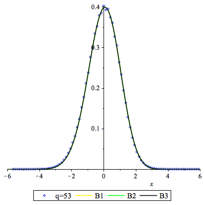
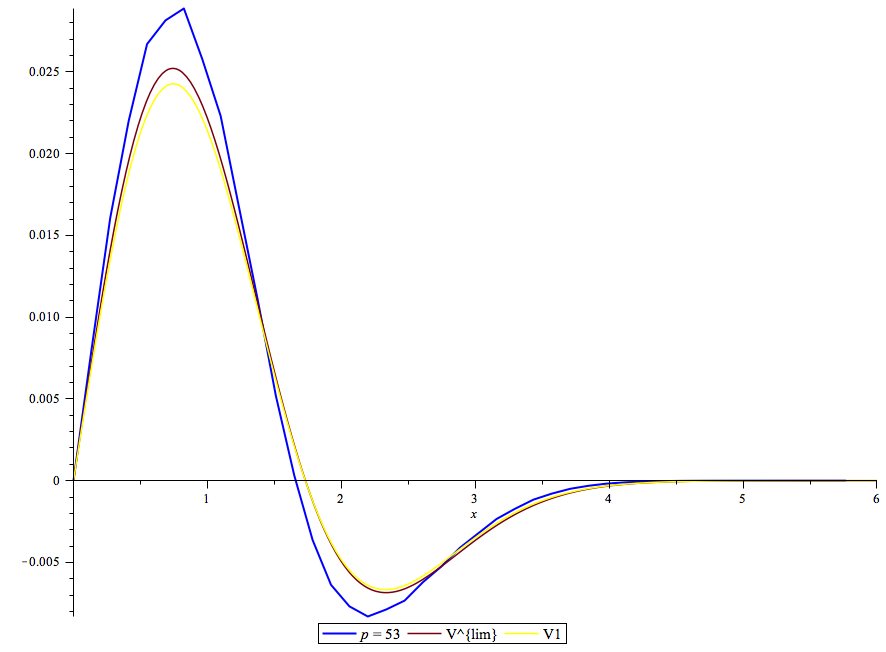
We can now make a graphical comparison of the experimental distribution of 𝒱q,3KS(x)superscriptsubscript𝒱𝑞3KS𝑥\mathcal{V}_{q,3}^{\textrm{KS}}(x) for the largest value of q𝑞q (to wit, q=53𝑞53q=53) with the results from Section 3. Interpolating the binomial coefficient as in Equation (2.1), which defined the function b𝑏b in Section 2, we define B1subscript𝐵1B_{1}, B2subscript𝐵2B_{2}, and B3subscript𝐵3B_{3} by

Bi(x):=σi(NNμiσix)μiNμiσix(1μi)N(Nμiσix),assignsubscript𝐵𝑖𝑥subscript𝜎𝑖binomial𝑁𝑁subscript𝜇𝑖subscript𝜎𝑖𝑥superscriptsubscript𝜇𝑖𝑁subscript𝜇𝑖subscript𝜎𝑖𝑥superscript1subscript𝜇𝑖𝑁𝑁subscript𝜇𝑖subscript𝜎𝑖𝑥B_{i}(x):=\sigma_{i}{N\choose N\mu_{i}-\sigma_{i}x}\mu_{i}^{N\mu_{i}-\sigma_{i}x}(1-\mu_{i})^{N-(N\mu_{i}-\sigma_{i}x)}\ , (4.2)

where N=q2+q+1𝑁superscript𝑞2𝑞1N=q^{2}+q+1 and

  1. (1)

    σ1=q1/q2subscript𝜎1𝑞1superscript𝑞2\sigma_{1}=\sqrt{q-1/q^{2}} and μ1=1/qsubscript𝜇11𝑞\mu_{1}=1/q (corresponding to Corollary 3.4, i.e., possibly singular plane quartics);

  2. (2)

    σ2=q(11q2+q+1)subscript𝜎2𝑞11superscript𝑞2𝑞1\sigma_{2}=\sqrt{q(1-\frac{1}{q^{2}+q+1})} and μ2=(q+1)/(q2+q+1)subscript𝜇2𝑞1superscript𝑞2𝑞1\mu_{2}=(q+1)/(q^{2}+q+1) (corresponding to Corollary 3.6, i.e., smooth plane quartics);

  3. (3)

    σ3=qsubscript𝜎3𝑞\sigma_{3}=\sqrt{q} and μ3=1/qsubscript𝜇31𝑞\mu_{3}=1/q (a simplified version of these models).

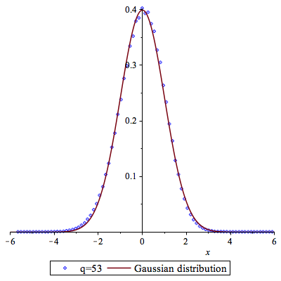
In both cases (1) and (2) we have blithely ignored the constraints on the degree that were required for the proofs of the corresponding results. Yet as Figure 3 shows, the plots of B1,B2,B3subscript𝐵1subscript𝐵2subscript𝐵3B_{1},B_{2},B_{3} and the Gaussian density function are almost indistinguishable, and all of these functions interpolate the distribution 𝒩53,3KS(x)subscriptsuperscript𝒩KS533𝑥\mathcal{N}^{\textrm{KS}}_{53,3}(x) quite well.

Refer to caption
(a) 𝒩53,3KS(x)subscriptsuperscript𝒩KS533𝑥\mathcal{N}^{\textrm{KS}}_{53,3}(x) against B1,B2,B3subscript𝐵1subscript𝐵2subscript𝐵3B_{1},B_{2},B_{3}
Refer to caption
(b) 𝒩53,3KS(x)subscriptsuperscript𝒩KS533𝑥\mathcal{N}^{\textrm{KS}}_{53,3}(x) against the Gaussian curve
Figure 3. Comparisons between 𝒩53,3KS(x)subscriptsuperscript𝒩KS533𝑥\mathcal{N}^{\textrm{KS}}_{53,3}(x) and its approximations.

As above, we are led to define

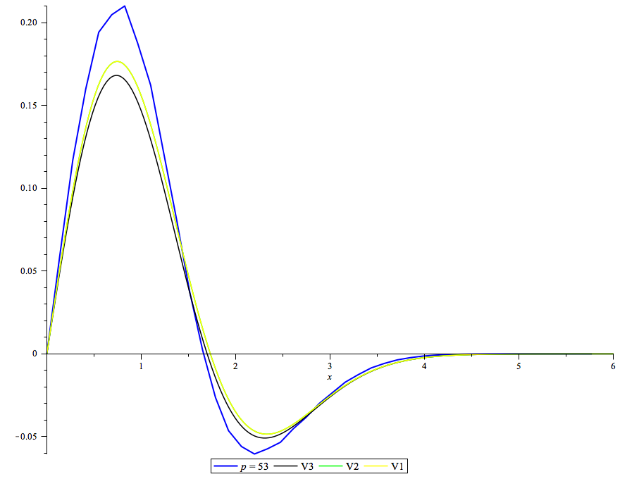
Vi(x):=σ(Bi(x)Bi(x))for i=1, 2, 3formulae-sequenceassignsubscript𝑉𝑖𝑥𝜎subscript𝐵𝑖𝑥subscript𝐵𝑖𝑥for 𝑖123V_{i}(x):=\sigma\,(B_{i}(x)-B_{i}(-x))\quad\text{for }i=1,\ 2,\ 3 (4.3)

and

Vlim(x):=132πx(3x2)ex2/2.assignsuperscript𝑉lim𝑥132𝜋𝑥3superscript𝑥2superscript𝑒superscript𝑥22V^{\textrm{lim}}(x):=\frac{1}{3\sqrt{2\pi}}x(3-x^{2})e^{-x^{2}/2}\ . (4.4)

This gives rise to the plots in Figure 4.

Refer to caption
(a) 𝒱53,3KS(x)subscriptsuperscript𝒱KS533𝑥\mathcal{V}^{\textrm{KS}}_{53,3}(x) against V1,V2,V3subscript𝑉1subscript𝑉2subscript𝑉3V_{1},V_{2},V_{3}
Refer to caption
(b) 𝒱53,3KS(x)subscriptsuperscript𝒱KS533𝑥\mathcal{V}^{\textrm{KS}}_{53,3}(x) against V1,Vlimsubscript𝑉1superscript𝑉limV_{1},V^{\textrm{lim}}
Figure 4. Comparisons between 𝒱53,3KS(x)subscriptsuperscript𝒱KS533𝑥\mathcal{V}^{\textrm{KS}}_{53,3}(x) and its approximations.

Once more we observe that the various curves closely resemble the distribution of 𝒱53,3KS(x)subscriptsuperscript𝒱KS533𝑥\mathcal{V}^{\textrm{KS}}_{53,3}(x). This time around, the agreement is all the more remarkable in that the limit distribution Vlimsuperscript𝑉limV^{\textrm{lim}} does not depend on any parameters, and hence cannot be adjusted.

5. Proof of Proposition 2.2

For notational convenience, throughout this proof we write N𝑁N, E𝐸E, μ𝜇\mu, m𝑚m, and n𝑛n for Nσsubscript𝑁𝜎N_{\sigma}, Eσsubscript𝐸𝜎E_{\sigma}, μσsubscript𝜇𝜎\mu_{\sigma}, m(σ,x)𝑚𝜎𝑥m({\sigma},x) and n(σ,x)𝑛𝜎𝑥n({\sigma},x).

Since E=σ2+1+O(1/σ2)𝐸superscript𝜎21𝑂1superscript𝜎2E=\sigma^{2}+1+O(1/\sigma^{2}) and x=o(σ)𝑥𝑜𝜎x=o(\sigma) at worst, we have

N𝑁\displaystyle N =σ4+O(σ2),absentsuperscript𝜎4𝑂superscript𝜎2\displaystyle=\sigma^{4}+O(\sigma^{2})\ ,
μ𝜇\displaystyle\mu =1σ2+O(1σ4),absent1superscript𝜎2𝑂1superscript𝜎4\displaystyle=\frac{1}{\sigma^{2}}+O\left(\frac{1}{\sigma^{4}}\right)\ ,
m𝑚\displaystyle m :=Eσx=σ2sσ+1+O(1σ2),assignabsent𝐸𝜎𝑥superscript𝜎2𝑠𝜎1𝑂1superscript𝜎2\displaystyle:=E-\sigma x=\sigma^{2}-s\,\sigma+1+O\left(\frac{1}{\sigma^{2}}\right)\ ,
n𝑛\displaystyle n :=(NE)+σx=Nm=σ4+O(σ2).assignabsent𝑁𝐸𝜎𝑥𝑁𝑚superscript𝜎4𝑂superscript𝜎2\displaystyle:=(N-E)+\sigma x=N-m=\sigma^{4}+O(\sigma^{2})\ .

Stirling’s approximation of the Gamma function

Γ(z+1)=2πz(ze)zeθzwith|θz|112zformulae-sequenceΓ𝑧12𝜋𝑧superscript𝑧𝑒𝑧superscript𝑒subscript𝜃𝑧withsubscript𝜃𝑧112𝑧\Gamma(z+1)=\sqrt{2\pi z}\left(\frac{z}{e}\right)^{z}e^{\theta_{z}}\quad\text{with}\quad{|\theta_{z}|}\leq\frac{1}{12z}

yields an approximation

b(σ,x)=12πNmn(Em)m(NEn)neθwithθ:=θNθmθn.formulae-sequence𝑏𝜎𝑥12𝜋𝑁𝑚𝑛superscript𝐸𝑚𝑚superscript𝑁𝐸𝑛𝑛superscript𝑒𝜃withassign𝜃subscript𝜃𝑁subscript𝜃𝑚subscript𝜃𝑛b(\sigma,x)=\frac{1}{\sqrt{2\pi}}\sqrt{\frac{N}{mn}}\left(\frac{E}{m}\right)^{m}\left(\frac{N-E}{n}\right)^{n}e^{\theta}\quad\text{with}\quad\theta:=\theta_{N}-\theta_{m}-\theta_{n}\ . (5.1)

Claims 1 through 6 below approximate the individual factors in Equation (5.1).

Claim 1: Nmn=1σ(1+x2σ+O(x2σ2))𝑁𝑚𝑛1𝜎1𝑥2𝜎𝑂superscript𝑥2superscript𝜎2\displaystyle\sqrt{\frac{N}{mn}}=\frac{1}{\sigma}\left(1+\frac{x}{2\sigma}+O\left(\frac{x^{2}}{\sigma^{2}}\right)\right).

Proof.

Note that

Nmn=1σ2×11+(2μ1)xσx2N=1σ2×11(1+O(1σ2))xσ+O(1σ2),𝑁𝑚𝑛1superscript𝜎2112𝜇1𝑥𝜎superscript𝑥2𝑁1superscript𝜎2111𝑂1superscript𝜎2𝑥𝜎𝑂1superscript𝜎2\frac{N}{mn}=\frac{1}{\sigma^{2}}\times\frac{1}{1+(2\,\mu-1)\frac{x}{\sigma}-\frac{x^{2}}{N}}=\frac{1}{\sigma^{2}}\times\frac{1}{1-(1+O\left(\frac{1}{\sigma^{2}}\right))\frac{x}{\sigma}+O\left(\frac{1}{\sigma^{2}}\right)}\ ,

and the Taylor expansion of the monotone function z1/1+zmaps-to𝑧11𝑧z\mapsto 1/\sqrt{1+z} yields Claim 1. ∎

Claim 2: eθ=1+O(1σ2)superscript𝑒𝜃1𝑂1superscript𝜎2\displaystyle e^{\theta}=1+O\left(\frac{1}{\sigma^{2}}\right).

Proof.

Estimating θ𝜃\theta, we have

|θ|=|θNθmθn|112|1N+Nnm|.𝜃subscript𝜃𝑁subscript𝜃𝑚subscript𝜃𝑛1121𝑁𝑁𝑛𝑚{|\theta|}={|\theta_{N}-\theta_{m}-\theta_{n}|}\leq\frac{1}{12}\left|\frac{1}{N}+\frac{N}{nm}\right|\ .

From Claim 1 and N=σ4+O(σ2)𝑁superscript𝜎4𝑂superscript𝜎2N=\sigma^{4}+O(\sigma^{2}) we obtain θ=O(1/σ2)𝜃𝑂1superscript𝜎2\theta=O(1/\sigma^{2}), which is enough to deduce Claim 2. ∎

We will approximate the product of the two middle terms of Equation (5.1) using

(Em)m(NEm)m=e(A+B)whereA:=ln(Em)mandB:=ln(NEn)n.\left(\frac{E}{m}\right)^{m}\left(\frac{N-E}{m}\right)^{m}=e^{-(A+B)}\quad\text{where}\quad A:=-\ln\left(\frac{E}{m}\right)^{m}\quad\text{and}\quad B:=-\ln\left(\frac{N-E}{n}\right)^{n}\ .

Claim 3: A=σx+x22+x361σ+O(x4σ2).𝐴𝜎𝑥superscript𝑥22superscript𝑥361𝜎𝑂superscript𝑥4superscript𝜎2\displaystyle A=-\sigma\,x+\frac{{x}^{2}}{2}+{\frac{{x}^{3}}{6}\,\frac{1}{\sigma}}+O\left(\frac{x^{4}}{\sigma^{2}}\right)\,.

Proof.

Indeed,

A=(Eσx)ln(EσxE)𝐴𝐸𝜎𝑥𝐸𝜎𝑥𝐸\displaystyle A=(E-\sigma x)\ln\left(\frac{E-\sigma x}{E}\right) =E(1σEx)ln(1σEx)absent𝐸1𝜎𝐸𝑥1𝜎𝐸𝑥\displaystyle=E\left(1-\frac{\sigma}{E}\,x\right)\ln\left(1-\frac{\sigma}{E}\,x\right)
=E(σEx+12(σEx)2+16(σEx)3+O((σEx)4)).absent𝐸𝜎𝐸𝑥12superscript𝜎𝐸𝑥216superscript𝜎𝐸𝑥3𝑂superscript𝜎𝐸𝑥4\displaystyle=E\left(-\frac{\sigma}{E}\,x+\frac{1}{2}\left(\frac{\sigma}{E}\,x\right)^{2}+\frac{1}{6}\left(\frac{\sigma}{E}\,x\right)^{3}+O\left(\left(\frac{\sigma}{E}\,x\right)^{4}\right)\right).

The claim follows because E=σ2+1+O(1/σ2)𝐸superscript𝜎21𝑂1superscript𝜎2E=\sigma^{2}+1+O(1/\sigma^{2}) and σ/E=1/σ1/σ3+O(1/σ5)𝜎𝐸1𝜎1superscript𝜎3𝑂1superscript𝜎5\sigma/E=1/\sigma-1/\sigma^{3}+O(1/\sigma^{5}). ∎

Claim 4: B=σx+x221σ2+O(x2σ4)𝐵𝜎𝑥superscript𝑥221superscript𝜎2𝑂superscript𝑥2superscript𝜎4\displaystyle B=\sigma\,x+\frac{{x}^{2}}{2}\,\frac{1}{\sigma^{2}}+O\left(\frac{x^{2}}{\sigma^{4}}\right).

Proof.

The proof is analogous to that of Claim 3, using B=(NE)(1+σNEx)ln(1+σNEx)𝐵𝑁𝐸1𝜎𝑁𝐸𝑥1𝜎𝑁𝐸𝑥B=(N-E)(1+\frac{\sigma}{N-E}\,x)\ln(1+\frac{\sigma}{N-E}\,x) and σ/(NE)=1/σ3+O(1/σ5)𝜎𝑁𝐸1superscript𝜎3𝑂1superscript𝜎5\sigma/(N-E)=1/\sigma^{3}+O(1/\sigma^{5}). ∎

Claim 5: A+B=x22+x361σ+O(x4σ2)𝐴𝐵superscript𝑥22superscript𝑥361𝜎𝑂superscript𝑥4superscript𝜎2\displaystyle A+B=\frac{{x}^{2}}{2}+{\frac{{x}^{3}}{6}\frac{1}{\sigma}}+O\left(\frac{x^{4}}{\sigma^{2}}\right).

Proof.

This is immediate from Claims 333 and 444. ∎

Claim 6: e(A+B)=ex22(1x36σ)+O(1σ2)superscript𝑒𝐴𝐵superscript𝑒superscript𝑥221superscript𝑥36𝜎𝑂1superscript𝜎2\displaystyle e^{-(A+B)}=e^{-\frac{x^{2}}{2}}\left(1-\frac{x^{3}}{6\sigma}\right)+O\left(\frac{1}{\sigma^{2}}\right).

Proof.

Taking a first-order Taylor approximation of the monotone function zezmaps-to𝑧superscript𝑒𝑧z\mapsto e^{z} shows that

ez=1+z+R(z),superscript𝑒𝑧1𝑧𝑅𝑧e^{z}=1+z+R(z)\ ,

where the remainder term R𝑅R satisfies |R(z)|(z2/2)e|z|𝑅𝑧superscript𝑧22superscript𝑒𝑧|R(z)|\leq(z^{2}/2)e^{|z|}. Thus

e(A+B)=ex22ex36σ+O(x4σ2)=ex22(1x36σ+O(x4σ2))+ex22R(x36σ+O(x4σ2)).superscript𝑒𝐴𝐵superscript𝑒superscript𝑥22superscript𝑒superscript𝑥36𝜎𝑂superscript𝑥4superscript𝜎2superscript𝑒superscript𝑥221superscript𝑥36𝜎𝑂superscript𝑥4superscript𝜎2superscript𝑒superscript𝑥22𝑅superscript𝑥36𝜎𝑂superscript𝑥4superscript𝜎2\displaystyle\begin{split}e^{-(A+B)}&=e^{-\frac{x^{2}}{2}}e^{-\frac{x^{3}}{6\sigma}+O\left(\frac{x^{4}}{\sigma^{2}}\right)}\\ &=e^{-\frac{x^{2}}{2}}\left(1-\frac{x^{3}}{6\sigma}+O\left(\frac{x^{4}}{\sigma^{2}}\right)\right)+e^{-\frac{x^{2}}{2}}R\left(-\frac{x^{3}}{6\sigma}+O\left(\frac{x^{4}}{\sigma^{2}}\right)\right)\ .\end{split}

The last term can be estimated by

|ex22R(x36σ+O(x4σ2))||(172σ2+O(1σ4))x6e(|x6σ+O(x2σ2)|12)x2|.superscript𝑒superscript𝑥22𝑅superscript𝑥36𝜎𝑂superscript𝑥4superscript𝜎2172superscript𝜎2𝑂1superscript𝜎4superscript𝑥6superscript𝑒𝑥6𝜎𝑂superscript𝑥2superscript𝜎212superscript𝑥2\left|e^{-\frac{x^{2}}{2}}R\left(-\frac{x^{3}}{6\sigma}+O\left(\frac{x^{4}}{\sigma^{2}}\right)\right)\right|\leq\left|\left(\frac{1}{72\sigma^{2}}+O\left(\frac{1}{\sigma^{4}}\right)\right)x^{6}e^{\left(\left|\frac{x}{6\sigma}+O\left(\frac{x^{2}}{\sigma^{2}}\right)\right|-\frac{1}{2}\right)x^{2}}\right|\ .

Here the assumption x=o(σ)𝑥𝑜𝜎x=o(\sigma) plays a role, bounding the product of the last factors as σ𝜎\sigma grows, so in fact a stronger estimate holds:

ex22R(x36σ+O(x4σ2))=O(1σ2).superscript𝑒superscript𝑥22𝑅superscript𝑥36𝜎𝑂superscript𝑥4superscript𝜎2𝑂1superscript𝜎2e^{-\frac{x^{2}}{2}}R\left(\frac{x^{3}}{6\sigma}+O\left(\frac{x^{4}}{\sigma^{2}}\right)\right)=O\left(\frac{1}{\sigma^{2}}\right).

Since x4ex22superscript𝑥4superscript𝑒superscript𝑥22x^{4}e^{-\frac{x^{2}}{2}} is also bounded, regardless of any growth assumptions on x𝑥x, we also have

ex22(O(x4σ2))=O(1σ2),superscript𝑒superscript𝑥22𝑂superscript𝑥4superscript𝜎2𝑂1superscript𝜎2e^{-\frac{x^{2}}{2}}\left(O\left(\frac{x^{4}}{\sigma^{2}}\right)\right)=O\left(\frac{1}{\sigma^{2}}\right)\ , (5.2)

which proves the claim. ∎

Putting all of our estimates together, we obtain a good approximation for b𝑏b as σ𝜎\sigma tends to infinity. First,

Nmneθ=1σ(1+x2σ+O(x2σ2))(1+O(1σ2))=1σ+x2σ2+O(x2σ3).𝑁𝑚𝑛superscript𝑒𝜃1𝜎1𝑥2𝜎𝑂superscript𝑥2superscript𝜎21𝑂1superscript𝜎21𝜎𝑥2superscript𝜎2𝑂superscript𝑥2superscript𝜎3\displaystyle\begin{split}\sqrt{\frac{N}{mn}}e^{\theta}&=\frac{1}{\sigma}\,\left(1+\frac{x}{2\sigma}+O\left(\frac{x^{2}}{\sigma^{2}}\right)\right)\left(1+O\left(\frac{1}{\sigma^{2}}\right)\right)\\ &=\frac{1}{\sigma}+\frac{x}{2\sigma^{2}}+O\left(\frac{x^{2}}{\sigma^{3}}\right)\ .\end{split}

Now consider the product

2πb(σ,x)=(1σ+x2σ2+O(x2σ3))e(A+B)=ex22(1σ+x2σ2+O(x2σ3))(1x36σ+O(1σ2));2𝜋𝑏𝜎𝑥1𝜎𝑥2superscript𝜎2𝑂superscript𝑥2superscript𝜎3superscript𝑒𝐴𝐵superscript𝑒superscript𝑥221𝜎𝑥2superscript𝜎2𝑂superscript𝑥2superscript𝜎31superscript𝑥36𝜎𝑂1superscript𝜎2\displaystyle\begin{split}\sqrt{2\pi}\,b(\sigma,x)&=\left(\frac{1}{\sigma}+\frac{x}{2\sigma^{2}}+O\left(\frac{x^{2}}{\sigma^{3}}\right)\right)e^{-(A+B)}\\ &=e^{-\frac{x^{2}}{2}}\left(\frac{1}{\sigma}+\frac{x}{2\sigma^{2}}+O\left(\frac{x^{2}}{\sigma^{3}}\right)\right)\left(1-\frac{x^{3}}{6\sigma}+O\left(\frac{1}{\sigma^{2}}\right)\right)\ ;\end{split} (5.3)

its main contribution is given by

ex22(1σ+x2σ2)(1x36σ)=ex22(1σx(x23)6σ2x412σ3).superscript𝑒superscript𝑥221𝜎𝑥2superscript𝜎21superscript𝑥36𝜎superscript𝑒superscript𝑥221𝜎𝑥superscript𝑥236superscript𝜎2superscript𝑥412superscript𝜎3e^{-\frac{x^{2}}{2}}\left(\frac{1}{\sigma}+\frac{x}{2\sigma^{2}}\right)\left(1-\frac{x^{3}}{6\sigma}\right)=e^{-\frac{x^{2}}{2}}\left(\frac{1}{\sigma}-{\frac{x\left({x}^{2}-3\right)}{6\,{\sigma}^{2}}}-{\frac{{x}^{4}}{12\,{\sigma}^{3}}}\right)\ .

As in the derivation of Equation (5.2), the final term in this sum is O(1/σ3)𝑂1superscript𝜎3O\left({1}/{\sigma^{3}}\right). The same technique shows that the other cross-terms in the product of Equation (5.3) are O(1/σ3)𝑂1superscript𝜎3O\left({1}/{\sigma^{3}}\right), which concludes the proof of Proposition 2.2.

References

  • [1] J. D. Achter, D. Erman, K. S. Kedlaya, M. Matchett Wood, and D. Zureick-Brown. A heuristic for the distribution of point counts for random curves over a finite field. Phil. Trans. R. Soc. A, 373(2040), 2015.
  • [2] A. Beauville and C. Ritzenthaler. Jacobians among abelian threefolds: a geometric approach. Math. Annal., 350(4):793–799, 2011.
  • [3] K. A. Behrend. The Lefschetz trace formula for algebraic stacks. Invent. Math., 112(1):127–149, 1993.
  • [4] P. Billingsley. Probability and measure. Wiley Series in Probability and Mathematical Statistics. John Wiley & Sons, Inc., New York, third edition, 1995. A Wiley-Interscience Publication.
  • [5] A. Bucur, C. David, B. Feigon, and M. Lalín. Fluctuations in the number of points on smooth plane curves over finite fields. J. Number Theory, 130(11):2528–2541, 2010.
  • [6] A. Bucur, C. David, B. Feigon, and M. Lalín. Statistics for traces of cyclic trigonal curves over finite fields. Int. Math. Res. Not. IMRN, (5):932–967, 2010.
  • [7] A. Bucur, C. David, B. Feigon, and M. Lalín. Biased statistics for traces of cyclic p𝑝p-fold covers over finite fields. In WIN—women in numbers, volume 60 of Fields Inst. Commun., pages 121–143. Amer. Math. Soc., Providence, RI, 2011.
  • [8] A. Bucur, C. David, B. Feigon, M. Lalín, and K. Sinha. Distribution of zeta zeroes of Artin-Schreier covers. Math. Res. Lett., 19(6):1329–1356, 2012.
  • [9] G. Cheong, M. Matchett Wood, and A. Zaman. The distribution of points on superelliptic curves over finite fields. Proc. Amer. Math. Soc., 143(4):1365–1375, 2015.
  • [10] A. Entin. On the distribution of zeroes of Artin-Schreier L-functions. Geom. Funct. Anal., 22(5):1322–1360, 2012.
  • [11] M. Homma and S. J. Kim. Nonsingular plane filling curves of minimum degree over a finite field and their automorphism groups: supplements to a work of Tallini. Linear Algebra Appl., 438(3):969–985, 2013.
  • [12] M. Homma and S. J. Kim. The second largest number of points of plane curves over finite fields, 2105. http://arxiv.org/abs/1509.02247.
  • [13] T. Ibukiyama. On rational points of curves of genus 333 over finite fields. Tohoku Math. J. (2), 45(3):311–329, 1993.
  • [14] N. M. Katz and P. Sarnak. Random matrices, Frobenius eigenvalues, and monodromy, volume 45 of American Mathematical Society Colloquium Publications. American Mathematical Society, Providence, RI, 1999.
  • [15] J. E. Kolassa. Series approximation methods in statistics, volume 88 of Lecture Notes in Statistics. Springer-Verlag, New York, second edition, 1997.
  • [16] P. Kurlberg and Z. Rudnick. The fluctuations in the number of points on a hyperelliptic curve over a finite field. J. Number Theory, 129(3):580–587, 2009.
  • [17] G. Lachaud and C. Ritzenthaler. On some questions of Serre on abelian threefolds. In Algebraic geometry and its applications, volume 5 of Ser. Number Theory Appl., pages 88–115. World Sci. Publ., Hackensack, NJ, 2008.
  • [18] G. Lachaud, C. Ritzenthaler, and A. Zykin. Jacobians among abelian threefolds: a formula of Klein and a question of Serre. Math. Res. Lett., 17(2), 2010.
  • [19] K. Lauter. The maximum or minimum number of rational points on genus three curves over finite fields. Compositio Math., 134(1):87–111, 2002. With an appendix by Jean-Pierre Serre.
  • [20] R. Lercier, C. Ritzenthaler, F. Rovetta, and J. Sijsling. Parametrizing the moduli space of curves and applications to smooth plane quartics over finite fields. LMS J. Comput. Math., 17(suppl. A):128–147, 2014.
  • [21] M. Matchett Wood. The distribution of the number of points on trigonal curves over 𝔽qsubscript𝔽𝑞\mathbb{F}_{q}. Int. Math. Res. Not. IMRN, (23):5444–5456, 2012.
  • [22] J.-F. Mestre. Courbes de genre 333 avec S3subscript𝑆3S_{3} comme groupe d’automorphismes, 2010. http://arxiv.org/abs/1002.4751.
  • [23] E. Nart and C. Ritzenthaler. Jacobians in isogeny classes of supersingular abelian threefolds in characteristic 2. Finite fields and their applications, 14:676–702, 2008.
  • [24] E. Nart and C. Ritzenthaler. Genus three curves with many involutions and application to maximal curves in characteristic 222. In Proceedings of AGCT-12, volume 521, pages 71–85. Contemporary Mathematics, 2010.
  • [25] B. Poonen. Bertini theorems over finite fields. Ann. of Math. (2), 160(3):1099–1127, 2004.
  • [26] C. Ritzenthaler. Aspects arithmétiques et algorithmiques des courbes de genre 111, 222 et 333. Habilitation à Diriger des Recherches, Université de la Méditerranée, 2009.
  • [27] C. Ritzenthaler. Explicit computations of Serre’s obstruction for genus-3 curves and application to optimal curves. LMS J. Comput. Math., 13:192–207, 2010.
  • [28] J.-P. Serre. Nombres de points des courbes algébriques sur 𝐅qsubscript𝐅𝑞{\bf F}_{q}. In Seminar on number theory, 1982–1983 (Talence, 1982/1983), pages Exp. No. 22, 8. Univ. Bordeaux I, Talence, 1983.
  • [29] A. B. Sørensen. On the number of rational points on codimension-111 algebraic sets in 𝐏n(𝐅q)superscript𝐏𝑛subscript𝐅𝑞{\bf P}^{n}({\bf F}_{q}). Discrete Math., 135(1-3):321–334, 1994.
  • [30] G. Tallini. Le ipersuperficie irriducibili d’ordine minimo che invadono uno spazio di Galois. Atti Accad. Naz. Lincei Rend. Cl. Sci. Fis. Mat. Nat. (8), 30:706–712, 1961.
  • [31] G. Tallini. Sulle ipersuperficie irriducibili d’ordine minimo che contengono tutti i punti di uno spazio di Galois Sr,qsubscript𝑆𝑟𝑞S_{r,q}. Rend. Mat. e Appl. (5), 20:431–479, 1961.
  • [32] G. van der Geer and M. van der Vlugt. Supersingular curves of genus 222 over finite fields of characteristic 222. Mathematische Nachrichten, 159:73–81, 1992.
  • [33] M. Xiong. The fluctuations in the number of points on a family of curves over a finite field. J. Théor. Nombres Bordeaux, 22(3):755–769, 2010.
  • [34] M. Xiong. Distribution of zeta zeroes for abelian covers of algebraic curves over a finite field. J. Number Theory, 147:789–823, 2015.