Transient dynamics of pulse-coupled oscillators with nonlinear charging curves

Abstract

We consider the transient behavior of globally coupled systems of identical pulse coupled oscillators. Synchrony develops through an aggregation phenomenon, with clusters of synchronized oscillators forming and growing larger in time. Previous work derived expressions for these time dependent clusters, when each oscillator obeyed a linear charging curve. We generalize these results to cases where the charging curves have nonlinearities.

I Introduction

During each heartbeat, thousands of pacemaker cells discharge in concert. This collective firing causes the contraction of cardiac muscles, which pump blood around the body. Should these firing fall out of step, heartbeats can become erratic, which inhibits blood flow. In order to maintain healthy heart function, the pacemaker cells must maintain their synchronous firing.

In 1975, Peskin gave the first mathematical analysis of the pacemaker as a self-synchronizing system Peskin (1975). He modeled the pacemaker cells as leaky ’integrate-and-fire’ oscillators that communicate with each other by firing sudden impulses. He then conjectured that a population of identical leaky oscillators with all-to-all pulsatile coupling would self-organize into synchrony for all $N\geq 2$ and for almost all initial conditions. Mirollo and Strogatz Mirollo and Strogatz (1990) later proved this conjecture.

Since then, pulse-coupled oscillators have been used as models in many other contexts, for example, sensor networks Hong and Scaglione (2003), low-powered radio transmission Wang and Apsel (2007), firing neurons Kirst et al. (2009); Ermentrout and Terman (2010), earthquakes Scholz (2010), and economic booms and busts Gualdi et al. (2015). For greater realism, the associated theoretical work relaxed Peskin’s original assumptions, allowing for local coupling in lattices or networks, non-instantaneous interactions, and so on Ernst et al. (1995); Gerstner (1996); Bressloff et al. (1997); Bressloff and Coombes (1998a); Corral et al. (1995); Bottani (1995); Timme et al. (2002a); Abbott and van Vreeswijk (1993); Timme et al. (2002b); Brunel (2000); Arenas et al. (2008); Bressloff and Coombes (1998b); Guardiola et al. (2000); Mauroy and Sepulchre (2008); Urbanczik and Senn (2001); Bressloff and Coombes (1998c); Brunel and Hakim (1999); Van Vreeswijk et al. (1994); Montbrió et al. (2015); Pazó and Montbrió (2014).

Yet even within the simplified context of Peskin’s all-to-all model, unanswered theoretical questions remain. In particular, little is known about transient dynamics: in a self-synchronizing system, what does the buildup to synchrony look like? A first step in this direction was presented in O’Keeffe et al. (2015). It was shown that synchrony developed through clustering; oscillators start to synchronize in small groups, which grow steadily larger over time. Using tools from aggregation theory Krapivsky et al. (2010), this clustering was described quantitatively. In the analysis, it was assumed that each oscillator had a linear charging curve. This idealization is appropriate for electronic oscillators such as those in sensor networks, but not for biological oscillators, like the aforementioned cardiac pacemaker cells or firing neurons. We here extend the analysis in O’Keeffe et al. (2015) to explore the manner in which these more complicated oscillators achieve synchrony.

II The model

We consider $N\gg 1$ identical oscillators coupled all-to-all. Each oscillator is characterized by a voltage-like state variable $x_{i}$, which increases from a baseline value of $0$ to a threshold set to 1, according to $\dot{x_{i}}=S_{0}-\gamma x_{i}$. When an oscillator reaches threshold it does two things: (i) It fires a pulse of size $1/N$. This pulse is received by all other oscillators instantaneously, causing them to discontinuously raise their voltage from $x_{j}$ to $\min(x_{j}+1/N,1)$. This way, oscillators never exceed the threshold value of $1$. To avoid complications with chain reactions of firing oscillators, we assume any oscillators which reach threshold by receiving a pulse, do not themselves fire until the next time they reach threshold. (ii) The firing oscillator then resets its voltage to $0$, along with any secondary oscillators that were brought to threshold. These oscillators then begin their next cycle synchronized.

If $j>1$ oscillators reach threshold together, each one fires, so that the pulse has total size $j/N$ (although we later consider other types of pulse).

We note that there is some parameter redundancy, since by rescaling time we could set $S_{0}=1$ without loss of generality. For reasons that will become clear later, a different choice of $S_{0}$ is more convenient, so we leave it as a free parameter for now. We remark however that $S_{0}$ must be chosen so that $\dot{x_{i}}>0$ for $0\leq x\leq 1$.

III Results

Assume the initial voltages of the oscillators are drawn uniformly at random. How will the dynamics unfold? At the beginning, the oscillators simply increase their voltage according to $\dot{x_{i}}=S_{0}-\gamma x_{i}$. Then the first oscillator reaches threshold, fires a pulse, and perhaps brings some other oscillators to threshold. As described, these oscillators begin their next cycle in step. The primary, firing oscillator, and the secondary oscillators it incited to threshold, form a synchronous cluster.

As time goes on, other oscillators start firing pulses and start absorbing oscillators which are close enough to threshold. More clusters of synchronized oscillators emerge. In turn, these clusters start reaching threshold and absorbing other clusters, growing progressively larger. We note that clusters can only ever increase in size. They can never break apart because (a) the oscillators are identical, and therefore sync’d oscillators have the same speed, and (b) all oscillators receive the same number of pulses (thanks to the global coupling).

The picture is now clear; the system synchronizes through an aggregation phenomenon. Clusters of sync’d oscillators form and get steadily bigger by coalescing with each other. At any time $t$ therefore, there are clusters of various sizes. Let $N_{j}(t)$ denote the number of clusters of size $j$ at time $t$: $N_{1}$ is the number of singletons, $N_{2}$ is the numbers doublets, and so on. These $N_{j}$ are correlated random quantities. They are correlated because oscillators belonging to clusters of one size are unavailable to clusters of another size, and they are random because of the initial conditions.

To analyze the system’s dynamics, we imagine $N_{j}\gg 1$ so that fluctuations from different realizations of the system are small. Of course, this condition cannot be satisfied for every $j$, at all $t$. For example, at the final stages of the process, there will be a small number of very large clusters. We therefore restrict our attention to the portion of the process where $N_{j}\gg 1$ is approximately true – the opening and middle game, as opposed to the end game.

But how does the end game play out? That is, how does the process terminate? Strogatz and Mirollo Mirollo and Strogatz (1990) showed that for $\gamma>0$ and pulse size $>1/N$, then full sync is guaranteed for all IC except for a set of measure zero; the clustering continues until there is one giant cluster of size $N$. For other values of $\gamma$ and other pulse sizes, full sync is possible, but not certain to occur.

In this work, we focus only on the transient dynamics, the evolution to synchrony. So from now on we implicitly assume we in the early and middle stages of the process, where $N_{j}\gg 1$ is a valid approximation. We then use ensemble averages to define the individual cluster densities,

$$c_{j}:=\langle N_{j}\rangle/N.$$ (1)

We then make the following strong assumptions: (i) fluctuations about the ensemble averages are small, $N^{-1}N_{j}=c_{j}+O(N^{-1/2})$, and that (ii) different cluster densities are asymptotically uncorrelated, $N^{-2}N_{i}N_{j}=c_{i}c_{j}+O(N^{-1/2})$.

We can use these $c_{j}$ to define a disorder parameter for our system. This is the total cluster density,

$$c=\sum_{j}c_{j}.$$ (2)

It measures of the total fragmentation of the system, which we interpret as a kind of disorder. To see this, consider that at $t=0$, there are $N$ singletons, so $c_{1}=1$, and $c_{j}=0,\;\forall j\neq 1$. This means that $c(0)=1$, correctly identifying that the system begins maximally disordered. At the other extreme as $t\rightarrow\infty$, we know there is one giant cluster of size $N$, so $c=1/N\approx 0$ for large $N$. Hence $c$ decreases from $1$ to $0$ as the system evolves from complete disorder to full synchrony.

III.1 Total Cluster Density

We first analyse $c$. It obeys the following rate equation, where $R_{i}$ is the rate at which clusters of size $i$ fire, and $L_{i}$ is the number of clusters absorbed during such a firing, for $i=1,\dots,N$:

$$\dot{c}=-\sum_{i}R_{i}(t)L_{i}(t)$$ (3)

To find $L_{i}(t)$, we first define the ’voltage-density’ $\rho_{j}(x,t)dx$ to be the number of $j$-clusters with voltage between $x$ and $x+dx$ at time $t$. This has the normalization condition $\int_{0}^{1}\rho_{j}(x,t)dx=N_{j}$. Now, when an $i$-cluster fires, all clusters on the interval $[1-i/N,1)$ will be absorbed. This means,

$$L_{i}(t)=\sum_{j}\int_{1-i/N}^{1}\rho_{j}(x,t)dx.$$ (4)

We now make an approximation. As stated earlier, we are only interested in transient time scales – the opening and middle game. In this regime, most clusters will be small relative to the system size: $j\ll N$. This lets us approximate the integral above, $\int_{1-i/N}^{1}\rho_{j}(x,t)dx\approx(i/N)\rho_{j}(x=1,t)$. Of course, this approximation will get worse as time goes on. We discuss this further in Section IV. Our expression for $L_{i}$ is then

$$L_{i}(t)=\frac{i}{N}\sum_{j}\rho_{j}(x=1,t)$$ (5)

To continue the analysis, we need to find $\rho_{j}(x,t)$. Its behavior is however complicated so we defer its calculation, and instead find the firing rate $R_{i}$. Naively, one might think that this is simply the flux of $i$-clusters at threshold: $N^{-1}(\rho_{i}v)|_{x=1}$ (where $N^{-1}$ is required, since $R_{i}$ measure the rate of firing of $c_{i}$, not $N_{i}$). However not every cluster that reaches threshold gets the chance to fire, since some will be absorbed. To account for this effect, we decompose the rate into

$$R_{i}=R_{i}^{0}-R_{i}^{a}.$$ (6)

The term $R_{i}^{0}$ is a ’background’ firing rate, where we pretend all oscillators get to fire even if they are absorbed. $R_{i}^{a}$ is the rate at which $i$-clusters are being absorbed by other clusters of various sizes, and hence deprived of their chance to fire.

We start with $R_{i}^{0}$. To be clear, by background firing rate, we mean the rate $i$-clusters would fire at, if every oscillator fired a pulse when it reached threshold. That is, imagine relaxing our imposition that any secondary oscillators that reach threshold by virtue of a pulse do not fire. In that case,

$$R_{i}^{0}=N^{-1}(\rho_{i}v)\big{|}_{x=1}.$$ (7)

The speed $v$ of each cluster is non-trivial. This is because in addition to its natural speed $v_{0}=\dot{x}=S_{0}-\gamma x$, each oscillator receives a steady stream of pulses from firing clusters which increase its voltage:

$$v(x,t)=v_{0}(x)+v_{pulse}(t).$$ (8)

This ”pulse velocity” due to the firing of just $j$-clusters will be (absolute number of pulses per sec) $\times$ (distance per pulse). Since $R_{j}$ is the firing rate of $c_{j}$, $R_{j}N$ is the absolute number of pulses, while the distance per pulse is $j/N$. To find the total pulse speed we then sum over all $j$-clusters: $\sum_{j}(NR_{j})(j/N)$, giving

$$v_{pulse}(t)=\sum_{j}jR_{j}(t).$$ (9)

Our next target is the absorption rate $R_{i}^{a}$. The calculation is similar to finding $L_{i}$, and is given by $R_{i}^{a}=\sum_{j}R_{j}\int_{1-j/N}^{1}\rho_{i}(x,t)dx$, which after approximating the integral as before gives,

$$R_{i}^{a}=\sum_{j}R_{j}(j/N)\rho_{i}(x=1,t).$$ (10)

Substituting $R_{i}^{0}$ and $R_{i}^{a}$ into (6) finally gives

$$R_{i}=\frac{S_{0}-\gamma}{N}\rho_{i}(x=1,t).$$ (11)

We now analyze $\rho_{j}(x,t)$. In principle, it satisfies the the continuity equation with appropriate terms for the absorption of $j$-clusters at threshold, and the formation of $j$-clusters from smaller clusters:

$$\dot{\rho_{j}}+\partial_{x}(v\rho_{j})+Absorption+Gain=0$$ (12)

$$\partial_{x}(v\rho_{j})|_{x=0}=\partial_{x}(v\rho_{j})|_{x=1}$$ (13)

This PDE is difficult to solve generally, given the non-smooth behavior of oscillators when they reach threshold. To proceed, we make the problem simpler, by observing that the evolution of the system naturally divides into periods $\{T_{n}\}$. We define a period to be the time take for the full population of oscillators to complete a voltage cycle. More carefully, $T_{n}$ is earliest time when every oscillator has completed $n$ cycles.

We then solve the continuity equation during a given period, not worrying about what happens before or after. This lets us avoid the complication of the non-smoothness of the oscillators’ behavior at the boundaries. We also neglect the absorption term. As previously discussed, when an $i$-cluster fires, only oscillators on $(1-i/N,1]$ get absorbed. This is a small interval for the ’opening’ and ’middle’ game we are considering. Hence the absorption term is $0$ on most of $[0,1]$ and so we omit it.

But we still have to compute the gain term. This would involve enumerating all the ways a $j$-cluster can be formed, which, as we will later show, is combinatorially intensive. We can however neglect this cumbersome term entirely, by making the following key observation.

Looking at equations (5), (11), we see our desired quantities $R_{j}$ and $L_{j}$ depend only on the density of clusters at threshold: $\rho_{j}(x=1,t)$. Therefore, during each period, $R_{i}$ and $L_{i}$ are only affected by $j$-clusters which existed at the start of that period, which we call ’original’ $j$-clusters. This is because any ’new’ $j$-clusters won’t reach threshold until the next period. By ’new’, we mean (a) $j$-clusters that fired during a period, didn’t absorb any other clusters, and so returned to threshold, and (b) any $j$-clusters that were created by the firing and absorption of other smaller clusters.

So for the purposes of calculating $\rho_{j}(x=1,t)$ during a given period, there is a ’lightcone’ between original and new $j$-clusters. We therefore need to solve the continuity equation for the original $j$-clusters only, for which the gain term in zero. The problem is then given by (14) below, where $v(x,t)$ is given by (8), $f_{0}(x)$ is the initial distribution of $\rho_{j}^{original}$, and the Heaviside functions $H(x),H(1-x)$ are included to confine the I.C. to the interval $[0,1]$.

$$\dot{\rho_{j}}^{original}+\partial_{x}(v\rho_{j}^{original})=0$$

$$\rho_{j}^{original}(x,0)=f_{0}(x)H(x)H(1-x)$$ (14)

We don’t yet know the speed $v(x,t)$. However its structure, $v(x,t)=v_{0}(x)+v_{pulse}(t)$, lets us derive an approximate solution for $\rho_{j}^{original}(x,t)$ given by (15) below. The derivation of this key result and the definition of $\Gamma(x,t)$ are shown in the Appendix.

$$\rho_{j}^{original}(x,t)=e^{\gamma t}f_{0}\Big{(}\Gamma(x,t)\Big{)}H\Big{(}\Gamma(x,t)\Big{)}H\Big{(}1-\Gamma(x,t)\Big{)}.$$ (15)

What all this means is, if we known $\rho_{j}^{original}(x,t)$ at the start of a period, then we know how it will evolve until that period ends. For later convenience, we introduce the following notation. Let $\tilde{x}$ denote that during a period, $x$ is held fixed at its value at the start of that period: $\tilde{x}=x(t=T_{n})$ for $T_{n}<t<T_{n+1}$.

We next make the strong assumption that clusters of all sizes are distributed uniformly in voltage on $[0,1)$ at the start of each period: $\rho_{j}(x,t=T_{n})=\tilde{N_{j}}$. Then in (15), $f_{0}(x)=\tilde{N_{j}}$. We discuss the legitimacy of making this assumption in Section IV.

The Heaviside functions make (15) look complicated. But really, they only enforce that the $\rho_{j}^{original}$ is zero before and after the first and last $j$-cluster respectively. We remark that as it stands, the solution (15) propagates into the unphysical $x\geq 1$ regime. But we of course restrict our attention to just $x\in[0,1]$.

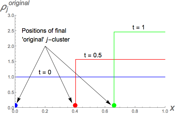
The behavior of $\rho_{j}^{original}(x,t)$ during each period is therefore simple. The density at each point $x$ simply grows at rate $e^{\gamma t}$ until it drops discontinuously to $0$, as the final ’original’ $j$-cluster passes by (by ’final’ we mean the $j$-cluster which had the lowest voltage at the start of the period). This behavior is shown in Figure 1.

Figure 1: Evolution of voltage density of original $j$-clusters during a period, with initial condition $\rho_{j}^{original}(x,0)=1$.

Now that we have an expression for $\rho_{j}(x=1,t)$, which we have argued is $\rho_{j}^{original}(x=1,t)$, we can complete our expressions for $L_{i}$ and $R_{i}$ given by (5) and (11). We then plug the results into (3) to obtain our sought after rate equation for the disorder parameter $c(t)$,

$$\dot{c}=-(S_{0}-\gamma)e^{2\gamma t}\tilde{c}.$$ (16)

which has solution,

$$c(t)=\frac{\tilde{c}}{2\gamma}\Big{(}S_{0}+\gamma+e^{2\gamma t}(\gamma-S_{0})\Big{)}.$$ (17)

We restate that equations (16) and (17) are only valid during a given period. We can however use (17) to find $c(t)$ for all $t$, by stitching solutions during successive periods together.

But we still don’t know the periods $\{T_{n}\}$ themselves. To find them, we need the speed $v$ as per (8). Recalling $v_{0}=S_{0}-\gamma x$, and substituting $R_{i}$ from (11), gives

$$v(x,t)=(S_{0}-\gamma x)+(S_{0}-\gamma)e^{\gamma t}.$$ (18)

We see that $v$ is the same during each period (i.e. there are no ’tilde’ quantities, we denote different values during different periods.). This means that the length of each period is the same: $T_{n}=nT_{0}$. We can find $T_{0}$ from $T_{0}(S_{0},\gamma)=\int_{0}^{1}v(x)dx$. To compare the effects of different amounts of concavity on equal footing, we want $T_{0}=1$ for every $\gamma$. We can achieve this by selecting an appropriate value for $S_{0}$, which we have strategically left as a free parameter thus far. Doing the integral, this value for $S_{0}$ is

$$S_{0}=\frac{\left(e^{2\gamma}+2e^{\gamma}-1\right)\gamma}{\left(e^{\gamma}-1\right)\left(e^{\gamma}+3\right)}.$$ (19)

We must be careful when using (19). This is because for sufficiently negative $\gamma$, $S_{0}$ can become negative. While we have ensured the total speed $v=v_{0}+v_{pulse}$ is positive, the natural speed $v_{0}=\dot{x}=S_{0}-\gamma x$ can become negative if $S_{0}$ is too negative. This means that the oscillators decrease in voltage in the absence of coupling. We avoid this unphysical regime by requiring $v_{0}>0$ for $0\leq x\leq 1$, which leads to $\gamma_{min}\approx-0.881$.

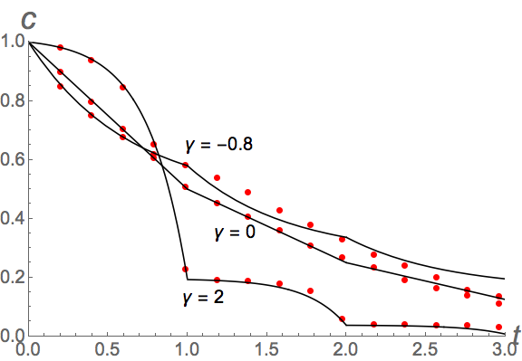
Figure 2 shows the agreement between theory and simulation for $\gamma<0$, $\gamma=0$, and $\gamma>0$. As can be seen, $c$ declines most rapidly when $\gamma>0$. This makes physical sense. When $\gamma>0$, oscillators slow down as they increase in voltage, which makes them clump closer together near $x=1$. When $\gamma<0$, the opposite happens; clusters spread further apart closer to threshold. Now suppose a $j$-cluster fires. When $\gamma>0$ the interval $[1-j/N,1)$ is more likely to contain oscillators than when $\gamma<0$, thanks to the ’clumping’ and ’spreading out’, which in turn makes an absorption more likely. The case of zero cavity, when $\gamma=0$, then interpolates between these two regimes, as evidenced by Figure 2.

Figure 2: (Color online) Theoretical and simulated $c(t)$ for $\gamma=2$, $\gamma=0$, and $\gamma=-0.8$ . Solid lines show theoretical prediction (17), while data points show simulated results for $N=5\times 10^{4}$ oscillators.

III.2 Individual Cluster Densities

How do the individual densities $c_{i}$ evolve? We begin with the $1$-clusters, whose density is $c_{1}$. They are the easiest density to analyze, since they can only decrease. There are two ways this can happen: (i) the loss of a firing singleton, when it absorbs other clusters of any size, and (ii) the loss of absorbed singletons, due to the firing of another cluster:

$$\dot{c_{1}}=\mathcal{L}_{1}^{firing}+\mathcal{L}_{1}^{absorbed}.$$ (20)

We begin with $\mathcal{L}_{1}^{firing}$. From (11) we know singletons fire at rate $R_{1}=(S_{0}-\gamma)e^{\gamma t}\tilde{c_{1}}$. During such a firing, an absorption will take place if there is at least one cluster on $[1-1/N,1)$. This interval contains on average $Nc\times 1/N=c(t)=\tilde{c}e^{\gamma t}$ clusters. Further, the probability that it contains $n$ clusters is given by the Poisson distribution: $\Pi_{n}=\frac{(\tilde{c}e^{\gamma t})^{n}}{n!}e^{-\tilde{c}e^{\gamma t}}$. The is the mathematical statement that the clusters are distributed randomly without correlations. The probability that $[1-1/N,1)$ is occupied by at least one cluster is therefore $1-e^{-\tilde{c}e^{\gamma t}}$. If an absorption takes place, $N_{1}$ decreases by $1$, since we’re only considering the loss of the firing oscillator here. The expected loss rate is then $(S_{0}-\gamma)e^{\gamma t}\tilde{c_{1}}[1\times(1-e^{-\tilde{c}e^{\gamma t}})+0\times e^{-\tilde{c}e^{\gamma t}}]$, leading to,

$$\mathcal{L}_{1}^{firing}=(S_{0}-\gamma)e^{\gamma t}\tilde{c_{1}}(1-e^{-\tilde{c}e^{\gamma t}}).$$ (21)

To calculate $\mathcal{L}_{1}^{absorbed}$, imagine a $j$-cluster fires and absorbs all the singletons on the interval $[1-j/N,1)$. As before, this interval will have on average $Nc_{1}(t)\times j/N=j\tilde{c_{1}}e^{\gamma t}$ such singletons. Multiplying this by $R_{j}$ and summing over $j$ then gives $\sum_{j}(1-\gamma)\tilde{c_{j}}e^{\gamma t}\times j\tilde{c_{1}}e^{\gamma t}$, which leads to

$$\mathcal{L}_{1}^{absorbed}=(1-\gamma)e^{2\gamma t}\tilde{c_{i}}$$ (22)

Substituting $\mathcal{L}_{1}^{firing}$ and $\mathcal{L}_{1}^{absorbed}$ into (20) gives,

$$\dot{c_{1}}=-(S_{0}-\gamma)\tilde{c_{1}}\Big{[}(1+e^{\gamma t})-e^{-\tilde{c}e^{\gamma t}}\Big{]}.$$ (23)

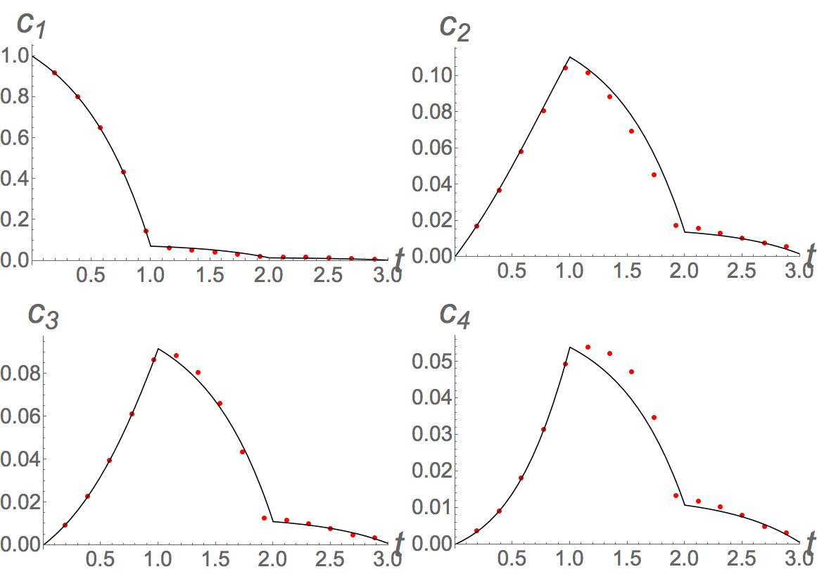
This looks intimidating, but since the quantities $\tilde{c_{i}}$ are held constant over each period, the R.H.S. is a function of only $t$. It therefore has an analytic solution, which we show plotted in Figure 3.

Will larger clusters behave similarly? They differ from the singletons in that they can be created as well as absorbed, which makes them harder to calculate. Their absorption rate is easily generalized from that of the singletons:

$$\mathcal{L}_{i}^{firing}+\mathcal{L}_{i}^{absorbed}=(S_{0}-\gamma t)\tilde{c_{i}}\Big{[}(1+e^{\gamma t})-e^{-i\tilde{c}e^{\gamma t}}\Big{]}.$$ (24)

Their gain rate is calculated as follows. A $i$-cluster is created when a cluster of size $k<i$ fires, and absorbs the right combination of other clusters. Suppose there are $a_{1}$ $1$-clusters, $a_{2}$ $2$-clusters, $\dots$, on the interval $[1-k/N,1)$. If $a_{1}+2a_{2}+\dots+k=i$, then an $i$-cluster will be created. Such a combination occurs with probability $\frac{(kc_{1})1^{a}_{1}}{a_{1}!}e^{-kc_{1}}\times\frac{(kc_{2})1^{a}_{2}}{a_{2}!}e^{-kc_{2}}\times\dots$. Summing first over all such combinations, and then over all $k$, gives an expected rate gain of

$$\sum_{k=1}^{i-1}(S_{0}-\gamma)\tilde{c_{k}}e^{\gamma t}e^{-k\tilde{c}e^{\gamma t}}\sum_{a_{1}+2a_{2}+\dots=i-k}\left(\prod_{p\geq 1}\frac{(k\tilde{c_{p}}e^{\gamma t})^{a_{p}}}{a_{p}!}\right)$$ (25)

After combining the loss and gain terms, and some algebraic manipulation, we finally obtain the desired rate equation for $i$-clusters,

$$\begin{split}\dot{c_{i}}&=-(S_{0}-\gamma)e^{\gamma t}(1+e^{\gamma t})\tilde{c_{i}}+\\ &\sum_{k=1}^{i}(S_{0}-\gamma)\tilde{c_{k}}e^{\gamma t}e^{-k\tilde{c}e^{\gamma t}}\sum_{\sum pa_{p}=i-k}\left(\prod_{p\geq 1}\frac{(k\tilde{c_{p}}e^{\gamma t})^{a_{p}}}{a_{p}!}\right)\end{split}$$ (26)

This is a set of recursive equations, and so we can solve them successively. As with $c_{1}$, the R.H.S. is a pure function of $t$, so analytic solutions are findable. Figure 3 show theoretical prediction versus simulation results.

Figure 3: (Color online) Theoretical and simulated cluster densities $c_{1}$ though $c_{4}$ for $\gamma=0.9$. Solid black lines show analytic solutions to (26). Red data points show simulations results for $5\times 10^{4}$ oscillators.

III.3 Alternate Coupling Rules

We thus far assumed an $i$-cluster fired a pulse of size $i/N$. We now consider two alternatives. The first is simply the original pulse strength with a tunable strength $K$: $(Ki)/N$. The second is a fixed pulse strength of $K/N$ regardless of the size of the firing cluster. These alterations only modestly change the analysis, so we simply list the results for $L_{i},R_{i},v_{pulse}$ and $c$ in the table below, where $S_{0}$ is given by (19). For illustrative purposes we do not include a formula for $c_{i}$, but its calculations is straightforward.

	$Kj/N$	$K/N$
$L_{i}$	$Ki\tilde{c}e^{\gamma t}$	$K\tilde{c}e^{\gamma t}$
$R_{i}$	$(S_{0}-\gamma)\tilde{c}_{i}e^{\gamma t}$	$(S_{0}-\gamma)\tilde{c}_{i}e^{\gamma t}$
$v_{pulse}$	$K(S_{0}-\gamma)e^{\gamma t}$	$K(S_{0}-\gamma)e^{\gamma t}\tilde{c}$
$c(t)$	$\frac{\tilde{c}\Big{(}K\left(\gamma-S_{0}\right)\left(e^{2\gamma t}-1\right)+2\gamma\Big{)}}{2\gamma}$	$\frac{\tilde{c}\Big{(}\tilde{c}K\left(\gamma-S_{0}\right)\left(e^{2\gamma t}-1\right)+2\gamma\Big{)}}{2\gamma}$

As can be seen, there are mostly only minor differences between the two cases. We remark however that $v_{pulse}$ now depends on $\tilde{c}$ for the fixed pulse case. This makes sense physically; since there are fewer clusters in successive periods, and the pulse per cluster is constant, the total ’current’ per period will get smaller. This is in contrast to the pulse = $Kj/N$ case, where there are fewer clusters per period also, but larger clusters fire larger pulses, keeping the total ’current’ per period constant. A consequence of this decrease in $v_{pulse}$ is that the periods won’t be constant for pulse $=K/N$, as there are for $Kj/N$. They will get longer as $v_{pulse}$ decreases from period to period.

IV Breakdown of Approximations

IV.1 Uniformity Assumption

We now discuss the approximations and assumptions we made in our analysis. The first of these was that each cluster density was distributed uniformly in voltage at the start of each period, $\rho_{j}(x,t)=\tilde{N_{j}}$. From this, we derived equations (5) and (11) for $L_{i}$ and $R_{i}$, which in turn led us to our disorder parameter $c$.

This uniformity assumption clearly cannot be satisfied for each $i$, at every $t$. For instance, consider the end of the first period. Perhaps mostly clusters of size $<5$ were formed, with only a few larger clusters of size $>10$. Then, $\rho_{j<5}(x,t=1)$ will be approximately uniform, but $\rho_{j}(x,t=1)$ will be more sharply peaked. So the uniformity assumption is inaccurate for large clusters, which are few in number. This explains why (17) approximates $c(t)$ well. Since $c(t)=\sum_{j}c_{j}$, we see that the sum will be dominated by those $c_{i}$ which are large, for which the uniformity assumption is accurate.

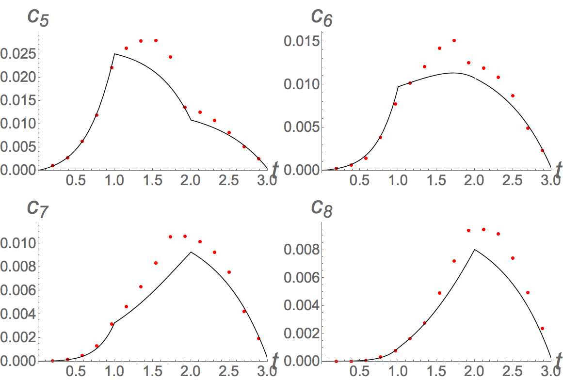
The fact that the uniformity assumption worsens for larger cluster sizes also means that our results for $c_{i}$ should get worse for larger $i$. Figure 4 below shows that this is indeed the case.

Figure 4: (Color online) Theoretical and simulated cluster densities $c_{5}$ though $c_{8}$ for $\gamma=0.9$. Solid black lines show analytic solutions to (26). Red data points show simulations results for $5\times 10^{4}$ oscillators. As can be seen, theory and simulation start to disagree

IV.2 Final stages of process

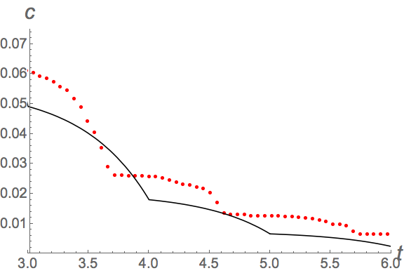
Throughout our analysis, we assumed $N_{j}\gg 1$. As previously discussed, this cannot be true for each $j$ at all times. This assumption is most blatantly incorrect during the final stages of the process, where there are a small number of macroscopic clusters. Our result should therefore substantially disagree with simulation for large enough $t$, as is evident in Figure 5.

Figure 5: (Color online) Theoretical and simulated total cluster density $c(t)$ for $\gamma=0.9$ and $t>3$. Solid black lines show analytic solution (2). Red data points show simulation results for $N=10^{4}$ oscillators. As can be seen, there is a significant disagreement between theory and simulation for later times, when the approximations we made in the analysis breakdown.

V Conclusion

We have studied the transient dynamics of pulse coupled oscillators with nonlinear charging curves. We derived approximations for the total cluster density $c(t)$ and individual cluster densities $c_{i}(t)$. These approximations were good up to the final stages of the process, where the assumptions made in the analysis breakdown.

A possible application of our results is in network detection. Arenas et al Gómez-Gardeñes et al. (2007) showed that transient clustering in the Kuramoto model can be used to approximate the underlying network structure. Could our results could be used to the same effect in networks of pulse-coupled oscillators? Local coupling would however mean that clusters could break apart as well as coalesce. One could account for this effect by including additional loss terms in our rate equations for $c$ and $c_{i}$, (3), (26).

Our model has several idealizations that could be relaxed in future work. For example, delay between emission and reception of pulses, heterogeneity in oscillator speeds and pulse sizes, and non-global coupling. Another interesting modification would be to allow chain reactions, by allowing any clusters that are brought to threshold by another firing cluster, to fire themselves.

VI Acknowledgments

This research was supported in part by the National Science Foundation through Grant No. DMS-1513179. We thank Steven Strogatz and Paul Krapivsky for helpful discussions.

VII Appendix

We here approximate the density $\rho_{j}^{original}(x,t)$. For convenience, we drop the superscript ’original’. As shown in the main body of the text, the density solves equation (27) below,

$$\dot{\rho_{j}}+\partial_{x}(v\rho_{j})=0$$

$$\rho_{j}(x,0)=f_{0}(x)H(x)H(1-x)$$ (27)

where, $f_{0}(x)=\tilde{N_{j}}$ (since we are assuming a initial uniform distribution), and

$$v(x,t)=v_{0}(x)+v_{pulse}(t).$$ (28)

While we know $v_{0}(x)=S_{0}-\gamma x$, we don’t yet have a complete expression for $v_{pulse}(t)$. In the main text, we derived $v_{pulse}=\sum_{j}jR_{j}$, which using (11) for $R_{i}$ gives

$$v_{pulse}(t)=\sum_{j}\frac{S_{0}-\gamma}{N}j\;\rho_{j}(x=1,t)$$ (29)

This is the source of our difficulty. Our PDE for $\rho_{j}(x,t)$ depends on $v_{pulse}$, which in turn depends on the voltage density for every other cluster size $\rho_{k}(x,t)$. To overcome this difficulty, we use a technique similar to the ’leap-frog’ or ’split’ method used in certain numerical schemes. This involves making a series of recursive approximations for $v_{pulse}$ and $\rho_{j}$:

$$v_{pulse} =\Big{(}v_{pulse}^{(0)},v_{pulse}^{(1)},v_{pulse}^{(2)},\dots\Big{)}$$ (30)

$$\rho_{j} =\Big{(}\rho_{j}^{(0)},\rho_{j}^{(1)},\rho_{j}^{(2)},\dots\Big{)}$$ (31)

Graphically, our scheme is given by the following, where we have placed the labels of equations used to make the approximations over the arrows.

$$v_{pulse}^{(0)}\xrightarrow{\eqref{cont_eqn2}}\rho_{j}^{(0)}\xrightarrow{\eqref{vp_step}}v_{pulse}^{(1)}\xrightarrow{\eqref{cont_eqn2}}\rho_{j}^{(1)}\xrightarrow{\eqref{vp_step}}+\dots$$ (32)

We begin by setting $v_{pulse}^{(0)}=0$. The speed is then,

$$v(x,t)^{(0)}=v_{0}(x)+0=S_{0}-\gamma x.$$ (33)

We plug this into (27) and solve for resulting PDE for $\rho_{j}^{(0)}(x,t)$. This has solution,

$$\rho_{j}^{(0)}(x,t)=e^{\gamma t}\tilde{N_{j}}H\Big{(}\Gamma_{0}(x,t)\Big{)}H\Big{(}1-\Gamma_{0}(x,t)\Big{)}.$$ (34)

with $\Gamma_{0}(x,t)=\gamma^{-1}[S_{0}-(S_{0}-\gamma x)e^{\gamma t}]$. We then use $\rho_{j}^{(0)}$ to find $v_{pulse}^{(1)}$ using (29), which gives

$$v_{pulse}^{(1)}=(S_{0}-\gamma)e^{\gamma t}\tilde{c}.$$ (35)

This completes the first step of our scheme. We then repeat the process to find $\rho_{j}^{(1)}$ and $v_{pulse}^{(2)}$. We use $v_{pulse}^{(1)}$ to update the speed,

$$\begin{split}v(x,t)^{(1)}&=v_{0}(x)+v_{pulse}^{(1)}\\ &=(S_{0}-\gamma x)+(S_{0}-\gamma)e^{\gamma t}\tilde{c}.\end{split}$$ (36)

and then plug this into (27) to obtain a PDE for $\rho_{j}^{(1)}$, which we solve to get,

$$\rho_{j}^{(1)}(x,t)=e^{\gamma t}\tilde{N_{j}}H\Big{(}\Gamma_{1}(x,t)\Big{)}H\Big{(}1-\Gamma_{1}(x,t)\Big{)}$$ (37)

where $\Gamma_{1}(x,t)=\Big{[}\frac{3S_{0}-\gamma}{2\gamma}+\frac{e^{\gamma t}}{2\gamma}\left(2\gamma x-2S_{0}\right)+\frac{e^{2\gamma t}}{2\gamma}\left(\gamma-S_{0}\right)\Big{]}$ .

Looking at (34) and (37), we see that $\rho_{j}^{(0)}$ and $\rho_{j}^{(1)}$ have the same functional form. They only differ in the arguments of the Heaviside function: $\Gamma_{0}(x,t)\neq\Gamma_{1}(x,t)$. This remarkable similarity between $\rho_{j}^{(0)}$ and $\rho_{j}^{(1)}$ has an important consequence: it ’closes’ our approximation scheme. We see this by substituting $\rho_{j}^{(1)}$ into (29) to find,

$$v_{pulse}^{(2)}=(S_{0}-\gamma)e^{\gamma t}\tilde{c}=v_{pulse}^{(1)},$$ (38)

which implies that $\rho_{j}^{(2)}=\rho_{j}^{(1)}$, which in turn implies our scheme terminates at $(v_{pulse},\rho_{j})=(v_{pulse}^{(2)},\rho_{j}^{(1)})$. Our final approximations for $v_{pulse}$ and $\rho_{j}(x,t)$ are then,

$$v_{pulse}(t)\approx(S_{0}-\gamma)e^{\gamma t}\tilde{c}$$ (39)

$$\rho_{j}(x,t)\approx e^{\gamma t}\tilde{N_{j}}H\Big{(}\Gamma(x,t)\Big{)}H\Big{(}1-\Gamma(x,t)\Big{)}$$ (40)

with $\Gamma(x,t)=\Big{[}\frac{3S_{0}-\gamma}{2\gamma}+\frac{e^{\gamma t}}{2\gamma}\left(2\gamma x-2S_{0}\right)+\frac{e^{2\gamma t}}{2\gamma}\left(\gamma-S_{0}\right)\Big{]}$ .

This concludes our analysis. We state bluntly that our approach is not rigorously justified. Its legitimacy is supported only by the agreement between our analytic results and numerical simulation. We hope future work will elucidate the cause of its efficacy.

References

- Peskin (1975) C. S. Peskin, Mathematical aspects of heart physiology (Courant Institute of Mathematical Sciences, New York University, 1975).
- Mirollo and Strogatz (1990) R. E. Mirollo and S. H. Strogatz, SIAM Journal on Applied Mathematics 50, 1645 (1990).
- Hong and Scaglione (2003) Y.-W. Hong and A. Scaglione, in Ultra Wideband Systems and Technologies, 2003 IEEE Conference on (IEEE, 2003), pp. 190–194.
- Wang and Apsel (2007) X. Y. Wang and A. B. Apsel, in Circuits and Systems, 2007. MWSCAS 2007. 50th Midwest Symposium on (IEEE, 2007), pp. 1524–1527.
- Kirst et al. (2009) C. Kirst, T. Geisel, and M. Timme, Physical review letters 102, 068101 (2009).
- Ermentrout and Terman (2010) G. B. Ermentrout and D. H. Terman, Mathematical foundations of neuroscience, vol. 35 (Springer Science & Business Media, 2010).
- Scholz (2010) C. H. Scholz, Bulletin of the Seismological Society of America 100, 901 (2010).
- Gualdi et al. (2015) S. Gualdi, J.-P. Bouchaud, G. Cencetti, M. Tarzia, and F. Zamponi, Physical review letters 114, 088701 (2015).
- Ernst et al. (1995) U. Ernst, K. Pawelzik, and T. Geisel, Phys. Rev. Lett. 74, 1570 (1995), URL http://link.aps.org/doi/10.1103/PhysRevLett.74.1570.
- Gerstner (1996) W. Gerstner, Physical review letters 76, 1755 (1996).
- Bressloff et al. (1997) P. C. Bressloff, S. Coombes, and B. de Souza, Phys. Rev. Lett. 79, 2791 (1997), URL http://link.aps.org/doi/10.1103/PhysRevLett.79.2791.
- Bressloff and Coombes (1998a) P. C. Bressloff and S. Coombes, Phys. Rev. Lett. 80, 4815 (1998a), URL http://link.aps.org/doi/10.1103/PhysRevLett.80.4815.
- Corral et al. (1995) A. Corral, C. J. Pérez, A. Díaz-Guilera, and A. Arenas, Phys. Rev. Lett. 74, 118 (1995), URL http://link.aps.org/doi/10.1103/PhysRevLett.74.118.
- Bottani (1995) S. Bottani, Phys. Rev. Lett. 74, 4189 (1995), URL http://link.aps.org/doi/10.1103/PhysRevLett.74.4189.
- Timme et al. (2002a) M. Timme, F. Wolf, and T. Geisel, Phys. Rev. Lett. 89, 258701 (2002a), URL http://link.aps.org/doi/10.1103/PhysRevLett.89.258701.
- Abbott and van Vreeswijk (1993) L. F. Abbott and C. van Vreeswijk, Phys. Rev. E 48, 1483 (1993), URL http://link.aps.org/doi/10.1103/PhysRevE.48.1483.
- Timme et al. (2002b) M. Timme, F. Wolf, and T. Geisel, Phys. Rev. Lett. 89, 154105 (2002b), URL http://link.aps.org/doi/10.1103/PhysRevLett.89.154105.
- Brunel (2000) N. Brunel, Journal of computational neuroscience 8, 183 (2000).
- Arenas et al. (2008) A. Arenas, A. Díaz-Guilera, J. Kurths, Y. Moreno, and C. Zhou, Physics Reports 469, 93 (2008).
- Bressloff and Coombes (1998b) P.C. Bressloff and S. Coombes, Physical Review Letters 81, 2168 (1998b).
- Guardiola et al. (2000) X. Guardiola, A. Diaz-Guilera, M. Llas, and C.J. Pérez, Physical Review E 62, 5565 (2000).
- Mauroy and Sepulchre (2008) A. Mauroy and R. Sepulchre, Chaos: An interdisciplinary journal of nonlinear science 18, 037122 (2008).
- Urbanczik and Senn (2001) R. Urbanczik and W. Senn, SIAM Journal On Applied Mathematics 61, 1143 (2001).
- Bressloff and Coombes (1998c) P.C. Bressloff and S. Coombes, Physical Review Letters 81, 2384 (1998c).
- Brunel and Hakim (1999) N. Brunel and V. Hakim, Neural computation 11, 1621 (1999).
- Van Vreeswijk et al. (1994) C. Van Vreeswijk, L. Abbott, and G. B. Ermentrout, Journal of computational neuroscience 1, 313 (1994).
- Montbrió et al. (2015) E. Montbrió, D. Pazó, and A. Roxin, Phys. Rev. X 5, 021028 (2015), URL http://link.aps.org/doi/10.1103/PhysRevX.5.021028.
- Pazó and Montbrió (2014) D. Pazó and E. Montbrió, Physical Review X 4, 011009 (2014).
- O’Keeffe et al. (2015) K. P. O’Keeffe, P. L. Krapivsky, and S. H. Strogatz, Phys. Rev. Lett. 115, 064101 (2015), URL http://link.aps.org/doi/10.1103/PhysRevLett.115.064101.
- Krapivsky et al. (2010) P. L. Krapivsky, S. Redner, and E. Ben-Naim, A kinetic view of statistical physics (Cambridge University Press, 2010).
- Gómez-Gardeñes et al. (2007) J. Gómez-Gardeñes, Y. Moreno, and A. Arenas, Phys. Rev. Lett. 98, 034101 (2007), URL http://link.aps.org/doi/10.1103/PhysRevLett.98.034101.
VII Appendix
We here approximate the density . For convenience, we drop the superscript ’original’. As shown in the main body of the text, the density solves equation (27) below,