The GTC exoplanet transit spectroscopy survey II

Abstract

Aims. We set to search for Rayleigh scattering and K and Na absorption signatures from the atmosphere of TrES-3b using ground-based transmission spectroscopy covering the wavelength range from 530 to 950 nm as observed with OSIRIS@GTC.

Methods. Our analysis is based on a Bayesian approach where the light curves covering a set of given passbands are fitted jointly with PHOENIX-calculated stellar limb darkening profiles. The analysis is carried out assuming both white and red – temporally correlated – noise, with two approaches (Gaussian processes and divide-by-white) to account for the red noise.

Results. An initial analysis reveals a transmission spectrum that shows a strong Rayleigh-like increase in extinction towards the blue end of the spectrum, and enhanced extinction around the K I resonance doublet near 767 nm. However, the signal amplitudes are significantly larger than expected from theoretical considerations. A detailed analysis reveals that the K I-like feature is entirely due to variability in the telluric O₂ absorption, but the Rayleigh-like feature remains unexplained.

1 Introduction

Transmission spectroscopy offers a powerful means for the characterisation of transiting exoplanet atmospheres. Measuring how the transit depth changes as a function of wavelength allows us to probe the existence and abundance of different atmospheric species – each with their wavelength-dependent extinction features – in the planet’s atmosphere (Seager & Sasselov, 2000; Brown, 2001). However, the variations in the transit depth are small, and high-altitude clouds can mask them altogether, leading to a flat transmission spectrum (Kreidberg et al., 2014; Berta et al., 2012). Further, atmospheric extinction is not the only source of wavelength-dependent features in transmission spectra, but stellar sources, such as star spots (Ballerini et al., 2012), plages (Oshagh et al., 2014), and flux contamination from an unresolved source can imprint features that can be difficult to disentangle from the atmospheric effects.

Since the colour variations in the transit depth are small – even in the absence of clouds – high-precision spectroscopic time series are required for meaningful analyses. Transmission spectroscopy has been most successful from space (Charbonneau et al., 2002; Sing et al., 2011; Gibson et al., 2012b, etc.), but the recent developments in observing techniques and modern data analysis methods have led to improvements in the precision that can be achieved from the ground. Simultaneous measurements of the target star and several comparison stars, similar to relative photometry (Bean et al., 2010; Gibson et al., 2012a), and the use of Gaussian processes, have facilitated the correction of systematics by allowing for the robust modelling of correlated noise – including time correlation and correlations with auxiliary measurements such as seeing – in model-independent fashion (Roberts et al., 2013; Gibson et al., 2012c; Rasmussen & Williams, 2006; Murgas et al., 2014).

We have observed a spectroscopic time series of a transit of TrES-3b, a massive hot Jupiter around a metal poor V=12.4 G-star on a 1.3 d orbit (see Table 1 and O’Donovan et al. 2007). The observations were carried out with the OSIRIS spectrograph (Optical System for Imaging and low-Intermediate-Resolution Integrated Spectroscopy; Sánchez et al., 2012) installed in the 10.4 m Gran Telescopio CANARIAS (GTC) in La Palma island. The observations cover the spectral range from 500 to 900 nm, probing the planet’s atmosphere for a possible Rayleigh scattering signal in the blue end of the spectrum, and the visible-light extinction features of the K I and Na I resonance doublets at 767 nm and 589.4 nm, respectively.

We detail our observations and data reduction procedures in (§2), the theoretical basis and the numerical methods in (§3), broadband (white) light curve modelling in (§4), transmission spectroscopy in (§5), and finally conclude with a discussion of the results (§6). The analysis and the raw data are publicly available on Github, as an easy-to-follow set of IPython notebooks and Python codes, to help with reproducibility of the study.

Table 1: Identifiers for TrES-3 with its coordinates and magnitudes.

Main identifiers
GSC ID	03089-00929
USNO-A2 ID	45017453
2MASS ID	J17520702+3732461
WASP ID	1SWASP J175207.01+373246.3
Equatorial coordinates
RA  (J2000)	$17^{h}\,52^{m}\,07\aas@@fstack{s}02$
Dec (J2000)	$+37\degr\,32\arcmin\,46\aas@@fstack{\prime\prime}2$
Magnitudes
Filter	Magnitude	Error
$B$	13.114	0.009
$V$	12.402	0.006
$R$	12.060	-
$I$	11.603	0.010
$J$	11.015	0.022
$H$	10.655	0.030
$K$	10.608	0.028

2 Observations

2.1 Overview

Observations were taken with OSIRIS@GTC on the night of 8 July 2014, during a transit of TrES-3b. A spectroscopic time series was taken in staring mode, from 1:27 to 4:00 UT, a total of 2.55 hours, starting 30 min before the ingress, and finishing 40 min after the egress, with a total of 255$\times$12 s exposures. Observing conditions were good, with median seeing at 0.86″, and the airmass varying from 1.06 to 1.56.

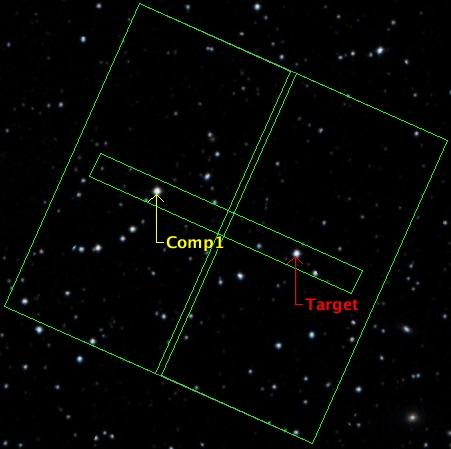
OSIRIS contains two 2048$\times$4096 pixel E2V CCDs, which were used in the 2$\times$2 binning mode. The observations were carried out using grism R1000R with a 40″-wide slit, with the target and a comparison star both located in the slit. We chose TYC~3089-995-1 as the comparison star, a star with a similar colour to TrES-3 and located at a distance of 3.93′ from it. The position angle of the reference star with respect to the target was 66°. The two stars were positioned equidistantly from the optical axis, close to the centre of each CCD, as shown in Fig. 1. The slit also includes several fainter stars, but these were found to be too faint to be useful in the data reduction. One of the faint stars (2MASS~17520839+3732378, see Sect. 2.4) is within a very short projected distance from TrES-3, and is included inside the aperture used to calculate the light curves. While the contaminating star is faint, its effect needs to be accounted for in the analysis.

Figure 1: Finding chart showing the field of view of OSIRIS and the slit position within the field (green boxes). The target star (TrES-3, right) and the comparison star (left) are also marked. Both OSIRIS CCDs were used for the observations, with one star located in each of the CCDs.

2.2 Generation of the spectra

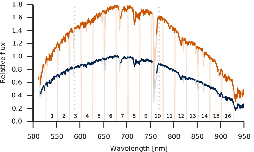
The 2D images were reduced to 1D spectra following the normal procedures for long-slit spectroscopy using routines within the IRAF environment. The raw spectra were bias corrected by subtracting the median-combined bias exposures and flat fielded by dividing by the normalised continuum lamp. Several apertures were tested for the optimal extraction, and the aperture that produced the white light curve with the smallest root mean square (RMS) scatter was finally chosen. For TrES-3b the aperture width was 50 binned pixels, which corresponds to 12.7″ on the detector (8.2 to 11.8 times the raw seeing during the observations). For TYC 3089-995-1 the aperture width was chosen to be 40 binned pixels, i.e. 10.16″ on the detector (6.5 to 9.6 times the raw seeing). Wavelength calibration was performed using the HgAr, Xe, Ne lamps for 1″-wide slit and a Chebyshev function fit of order 6, providing RMS better than 0.04 Å. Final spectra were not corrected for instrumental response nor flux calibrated. Fig. 2 shows the example spectra for the two stars used in time series analysis.

Figure 2: Sky-subtracted, wavelength-calibrated, spectra for TrES-3 (dark blue line, below) and the simultaneously observed comparison star (orange line, above), both normalised with an arbitrary but common normalisation factor. The parts masked out during the generation of spectrum-masked light curves (see below) are shown with a lighter shade, and the light-orange vertical lines show the ranges used to generate the 16 narrow-band light curves. The dotted vertical lines show the Ka I and Na I resonance doublets.

2.3 Light curve generation

Basic light curve set without spectrum masking

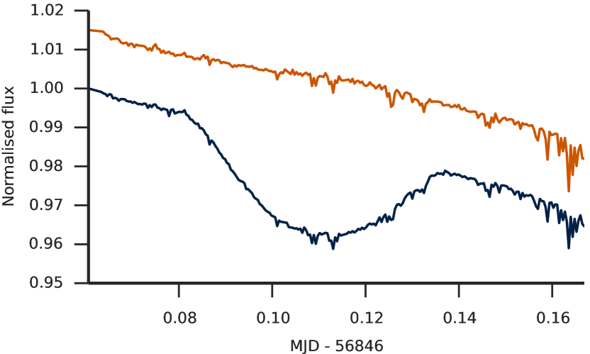
Two sets of light curves, with and without spectrum masking, were created from the raw spectra for each star. First, we carried out an initial analysis using a basic (unmasked) light curve set with a broadband light curve (Fig. 3) integrating the flux over the whole usable spectral range from 530 to 930 nm, and 16 narrow-band ($\sim$25 nm) light curves integrated over the spectral ranges shown in Fig. 2.

Light curve set with spectrum masking

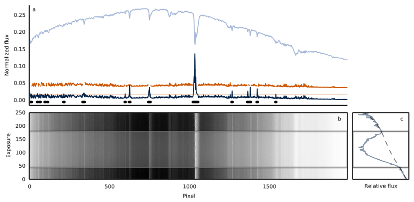
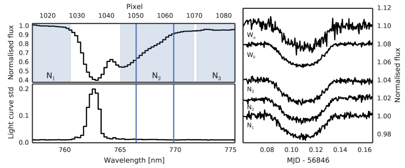
We realised during the initial analysis that the spectral regions corresponding to the cores of telluric absorption bands added a significant amount of noise to the narrow-band light curves. This was especially the case with the deep telluric O₂ absorption band near 760 nm. This motivated us to create a second set of light curves to assess how these spectrum regions affected the light curves, and, finally, our parameter estimates.

The masked light curve set was created by first calculating the standard deviations of detrended (using a simple fourth-order polynomial) light curves created for each wavelength element (pixel) for TrES-3 and the comparison star (Fig. 4). Next, we masked the wavelength elements where the noise level is higher than a given maximum noise level, and then proceeded as with the generation of the basic light curve set.

Spectrum masking was found to decrease the rms scatter in the narrow-band light curves covering telluric absorption bands, as illustrated in Fig. 5 for the strong O₂ absorption band, and the masked light curve set was adopted as the main analysis dataset.

Final transit light curves

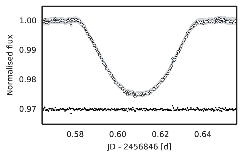
The final light curve sets were created by dividing the TrES-3 light curve sets (unmasked and masked) by the comparison star light curves. The rms scatter for the broadband curve is $\sim$500 ppm, with a white noise estimate (using Gaussian processes with an exponential kernel to model the time-correlated noise) of $\sim$350 ppm.

Figure 3: Raw broadband light curves for TrES-3 (below) and the simultaneously observed comparison star (above). The light curves are normalised to their first datapoint, and the comparison star’s light curve is shifted vertically for clarity.

Figure 4: Spectrum masking: a) TrES-3 spectrum (light-blue line), out-of-transit (OOT) standard deviation ($\sigma_{\mathrm{O}}$) of a detrended light curve created using a single spectral pixel (dark-blue line), maximum allowed $\sigma_{\mathrm{O}}$ (light-orange horizontal line), OOT standard deviation with a mask (orange line), masked locations (thick black lines in the bottom); b) the whole spectroscopic time series, time in the y-axis and wavelength (without wavelength calibration) in the x-axis, inside-transit duration marked between the two horizontal lines; c) broadband light curve with a fourth-order polynomial fitted to the OOT fluxes.

Figure 5: Upper-left panel: a close-up to TrES-3 spectrum with the K I resonance double lines marked as two vertical blue lines, and three passbands used to generate the narrow-band light curves in the panel on the right marked as light-blue shaded areas. Lower-left panel: a scatter map based on light curves generated using one pixel in the wavelength axis. Right: Light curves generated by integrating over the whole spectral range shown in the left panels (W_a), integrating over the three marked passbands (W_b, that is, excluding the core of the telluric O₂ absorption band), and integrated over the individual passbands (N₁–N₃).

2.4 Background Contamination

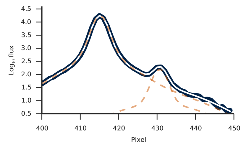
The aperture used to calculate the flux of TrES-3 includes a faint background star (2MASS 17520839+3732378, V=18.5). The star was estimated to contribute $\sim$1% of the total flux using PSF fitting. The fitting was done using four and three Gaussian components for the TrES-3 and the contaminant PSFs, respectively, as shown in Fig. 6. The contaminant is slightly redder than TrES-3b ($J-K=0.8$, while for TrES-3 $J-K=0.4$), and we give a (very conservative) constraints on its effective temperature to lie between 3500 and 5000 K. This temperature is used as a uniform prior later in the analysis.

Figure 6: Estimation of the contamination from the faint background star within the TrES-3 aperture. The thick black line shows the observed flux, the white line the fitted model, and the dashed orange lines the two model components.

3 Theory and numerical methods

3.1 Overview

The analysis consists of a basic broadband parameter estimation run carried out as a consistency test, and a transmission spectroscopy run for the 16 narrow passbands shown in Fig. 2. The approach for the parameter estimation is Bayesian: we use Markov chain Monte Carlo (MCMC) to obtain a representative sample from a model parameter posterior distribution, where the model jointly describes the observed light curves and a stellar limb darkening profile created using the PHOENIX stellar atmosphere library by Husser et al. (2013).

The model is parametrised with a parameter vector $\boldsymbol{\theta}$. A set of model parameters are passband-independent by nature, such as the transit centre and the impact parameter, and each passband adds a set of passband-dependent parameters, all listed in Table 2 with their priors. Thus, the number of parameters varies from 10 (broadband light curve assuming white noise), to $\sim$100 (16 narrow passbands, red noise).

Table 2: Parametrisation and priors. The uninformative priors are uniform and wide enough not to affect the posteriors. $N(\mu,\sigma)$ stands for a normal prior with mean $\mu$ and standard deviation $\sigma$. The colour dependent parameters are per passband.

Notation		Name	Prior
Informative priors
$\theta_{\mathrm{p}}$	$P$	orbital period	$N(1.306,10^{-7})$
Uninformative priors, colour independent
$\theta_{\mathrm{tc}}$	$T_{c}$	transit centre
$\theta_{\mathrm{\rho}}$	$\rho_{\star}$	stellar density
$\theta_{\mathrm{b}}$	$b$	impact parameter
$\theta_{\mathrm{Go}}$	$e$	GP output scale
$\theta_{\mathrm{Gi}}$	$l$	GP input scale
Uninformative priors, colour dependent
$\theta_{\mathrm{k}}$	$k$	radius ratio
$\theta_{\mathrm{u}}$	$u$	limb darkening u
$\theta_{\mathrm{v}}$	$v$	limb darkening v
$\theta_{\mathrm{B}}$	$B$	baseline level
$\theta_{\mathrm{x}}$	$x$	extinction coefficient
$\theta_{\epsilon}$	$\epsilon$	average white noise

The parameter estimation from the narrow-band light curves was carried out separately for three noise-models: WN) white and normally distributed noise; DW) red noise with a wavelength-independent systematic component; and GP) red noise described by a Gaussian process with time as the only input parameter. The broadband modelling used only WN and GP approaches. The likelihoods equations for each of these cases are detailed in Sect. 3.4.

Our parameter estimates correspond to the posterior median, and the uncertainties correspond to the 68% central posterior intervals, unless otherwise specified. We adopt the red noise results as our final results, due to their robustness over the white-noise assumption, but also describe any differences between the two.

The analysis relies on Python- and Fortran-based code utilising SciPy, NumPy (van der Walt et al., 2011), IPython (Perez & Granger, 2007), Pandas (Mckinney, 2010), matplotlib (Hunter, 2007), seaborn, PyFITS, and F2PY (Peterson, 2009). The transits were modelled with PyTransit (Parviainen, 2015), the limb darkening computations were carried out with PyLDTk, global optimisation was carried out with PyDE, the MCMC sampling was carried out with emcee (Foreman-Mackey et al., 2013; Goodman & Weare, 2010), and the Gaussian Processes were computed using George (Ambikasaran et al., 2014).

3.2 Limb darkening

TrES-3b presents a nearly grazing transit, and its inclined orbit leads to a degeneracy between the planet-star radius ratio, impact parameter and stellar limb darkening. When observing TrES-3b, O’Donovan et al. (2007) used multicolour photometry to break the degeneracy between the radius ratio and the impact parameter, allowing them to constrain the two, but they fixed the limb darkening coefficients to values tabulated in Claret (2004). These tabulations have been shown to disagree with observed limb darkening profiles (Claret, 2008, 2009), and fixing the limb darkening coefficients to the tabulated values can lead to biased parameter estimates with underestimated uncertainties. Nowadays, more robust approaches to account for limb darkening are widely used. The tabulations can be used to construct informative priors on the limb darkening coefficients, where the prior widths depend both on how much we trust the stellar models behind the tabulations and how well the host star has been characterised. The limb darkening coefficients can also be completely unconstrained in the parameter estimation, with uninformative priors, which leads to the most conservative parameter estimates.

We use an approach where, instead of constraining the limb darkening model coefficients, we constrain the shape of the stellar limb darkening profile. This is achieved by fitting a stellar limb darkening profile (with uncertainties propagated from the uncertainties in our stellar parameter estimates) created using the specific intensity spectra library by Husser et al. (2013) jointly with the light curves. The Husser et al. (2013) library allows us to create limb darkening profiles for freely defined passbands, and the profile-based approach reduces the problems encountered with the limb darkening coefficient correlation.

3.3 Transmission spectroscopy

The number of model parameters for the narrow-band analysis is $\sim$100, which means that the size of the parameter vector population has to be increased for the affine invariant sampler to work. Also, even then, the autocorrelation length of the chains is significantly higher than for the lower-dimensional white-light analysis, and more iterations are required to obtain a usable set of independent posterior samples. A small run was carried out to test whether fixing the GP hyperparameters affects the parameter estimates, and no significant effects were observed.

3.4 Posteriors and likelihoods

We model the observed spectrophotometry and the theoretical stellar intensity profiles jointly. Our unnormalised log posterior density is

$$\ln P(\boldsymbol{\theta}|D)=\ln P(\boldsymbol{\theta})+\ln P(\@vec{D_{\mathrm{LC}}}|\boldsymbol{\theta})+\ln P(\@vec{D_{\mathrm{LD}}}|\boldsymbol{\theta}),$$ (1)

where $\boldsymbol{\theta}$ is the parameter vector encapsulating all the model parameters, $\ln P(\boldsymbol{\theta})$ is the log prior, $\@vec{D_{\mathrm{LC}}}$ is the spectrophotometry data, $\ln P(\@vec{D_{\mathrm{LC}}}|\boldsymbol{\theta})$ is the log likelihood for the photometry, $\@vec{D_{\mathrm{LD}}}$ are the theoretical limb darkening profiles, and $\ln P(\@vec{D_{\mathrm{LD}}}|\boldsymbol{\theta})$ is the log likelihood for the limb darkening profiles.

Assuming that the uncertainties in the observations are normally distributed, we can write the general log likelihood for data $\@vec{D}$ given the parameter vector $\boldsymbol{\theta}$ in a vector form as

$$\ln P(\@vec{D}|\boldsymbol{\theta})=-\frac{1}{2}\left(n_{D}\ln 2\pi+\ln|\boldsymbol{\Sigma}|+\@vec{r}^{\mathrm{T}}\boldsymbol{\Sigma}^{-1}\@vec{r}\right),$$ (2)

where $n_{D}$ is the number of datapoints, $\@vec{r}$ is the residual vector with elements $r_{i}=D_{i}-M(t_{i},\boldsymbol{\theta})$, $M$ is the model, and $\boldsymbol{\Sigma}$ is the covariance matrix.

If the noise can be assumed white (that is, uncorrelated), the covariance matrix is diagonal, and the computation of the likelihood is trivial. However, if the noise is correlated, the covariance matrix will have off-diagonal elements, and the matrix needs to be inverted for the likelihood evaluation.

Likelihood for the stellar limb darkening profile

Instead of relying on the tabulated limb darkening coefficients, we model stellar intensity profiles calculated for TrES-3 and our passbands using the PHOENIX stellar atmosphere code jointly with the photometric data. This allows us to marginalise over the whole limb darkening coefficient space that can explain the theoretical stellar intensity (limb darkening) profile, and may yield more robust parameter estimates than by using fitted limb darkening coefficients directly.

The stellar limb darkening profile data, $\@vec{D_{\mathrm{LD}}}$, is constructed from stellar limb darkening profiles calculated using the PHOENIX code for 27 stellar parameter sets over 16 passbands (corresponding to the ones in our basic spectroscopic analysis) and 75 values of $\mu$ (where $\mu=\cos\gamma=\sqrt{1-z^{2}}$, $\gamma$ is the foreshortening angle, and $z$ is the projected distance from the centre of the stellar disk divided by the stellar radius). Let $I_{i,j}$ be the mean stellar intensity (averaged over the different stellar parameter sets) for passband $i$ and $\mu_{j}$, and $\sigma_{I,i,j}$ the corresponding standard deviation (uncertainty) of the stellar intensity, and $\epsilon$ a multiplicative factor $\geq 1$ to account for the fact that the numerical stellar models used to calculate the limb darkening profiles should not be relied on blindly (e.g., Claret, 2009). The uncertainties are independent, and the log likelihood can be written in scalar form as

$$\ln P(\@vec{D_{\mathrm{LD}}}|\boldsymbol{\theta})=-\sum_{i=1}^{n_{\mathrm{pb}}}\left(\frac{n_{\mathrm{\mu}}}{2}\ln 2\pi+\sum_{j=1}^{n_{\mathrm{\mu}}}\ln\epsilon\sigma_{\mathrm{I},i,j}+\frac{\chi^{2}_{i}}{2\epsilon^{2}}\right),$$ (3)

where

$$\chi^{2}_{i}=\sum_{j=1}^{n_{\mathrm{\mu}}}\frac{\left(I_{i,j}-M_{\mathrm{I}}(\mu_{j},\boldsymbol{\theta})\right)^{2}}{\sigma_{\mathrm{I},i,j}^{2}},$$ (4)

$n_{\mathrm{pb}}$ is the number of passbands, $n_{\mathrm{\mu}}$ the number of $\mu$-datapoints per passband (in this case a constant), and $M_{\mathrm{I}}$ is the limb darkening model.

We chose to use the quadratic limb darkening model (Mandel & Agol, 2002; Giménez, 2006)

$$M_{\mathrm{I}}(\mu,\boldsymbol{\theta})=1-\theta_{\mathrm{u}}(1-\mu)-\theta_{\mathrm{v}}(1-\mu)^{2}$$ (5)

after running test simulations with a quadratic and a general four-parameter limb darkening model (Giménez, 2006). The use of four-parameter model did not affect the parameter estimates (within the estimate uncertainties), but introduced unjustified complexity to the model with two additional parameters per passband.

Likelihood for the photometry assuming white noise

If we assume the noise in the photometry for a single passband to be i.i.d. (independent and identically distributed) from a zero-centred normal distribution with a standard deviation $\sigma_{\mathrm{lc,i}}$, the likelihood can be written out explicitly in scalar form as

$$\ln P(\@vec{D_{\mathrm{LC}}}|\boldsymbol{\theta})=-\sum_{i=1}^{n_{\mathrm{pb}}}\left(\frac{n_{\mathrm{ph}}}{2}\ln 2\pi\sigma_{\mathrm{lc,i}}^{2}+\sum_{j=1}^{n_{\mathrm{ph}}}\frac{\left(F_{j}-M_{\mathrm{P}}(\boldsymbol{\theta},t_{j},X)\right)^{2}}{2\sigma_{\mathrm{lc,i}}^{2}}\right)$$ (6)

where $n_{\mathrm{pb}}$ is the number of passbands, $n_{\mathrm{ph}}$ the number of photometric datapoints, and $\sigma_{\mathrm{lc,i}}$ the average scatter in the $i$th passband.

The photometry is modelled as a product of a baseline and a transit components as

$$M_{\mathrm{P}}(\boldsymbol{\theta},t,X)=\theta_{\mathrm{B}}\;e^{-\theta_{\mathrm{x}}X}\;T(t,\theta_{\mathrm{tc}},\theta_{\mathrm{p}},\theta_{\mathrm{k}},\theta_{\mathrm{a}},\theta_{\mathrm{i}},\theta_{\mathrm{e}},\theta_{\mathrm{\omega}},\theta_{\mathrm{u}},\theta_{\mathrm{v}})$$ (7)

where $\theta_{\mathrm{B}}$ is a constant baseline level, $X$ is the airmass, $\theta_{\mathrm{x}}$ is the (residual) extinction coefficient, $T$ is the transit model, $t$ is the mid-exposure time, $\theta_{\mathrm{tc}}$ is the zero epoch, $\theta_{\mathrm{p}}$ is the orbital period, $\theta_{\mathrm{k}}$ the planet-star radius ratio, $\theta_{\mathrm{a}}$ the scaled orbital semi-major axis, $\theta_{\mathrm{i}}$ the inclination, $\theta_{\mathrm{e}}$ the orbital eccentricity, $\theta_{\mathrm{\omega}}$ the argument of the periastron, and $\theta_{\mathrm{u}}$ and $\theta_{\mathrm{v}}$ are the quadratic limb darkening coefficients.

The baseline includes a constant baseline level and an atmospheric extinction term to model uncorrected extinction as a function of the airmass. The latter term is necessary since TrES-3 and the comparison star have a slightly different colour. The baseline parameters are passband dependent, and thus yield two free parameters per modelled passband. The transit is modelled using PyTransit, which is optimised for efficient modelling of spectrophotometric transits. A part of the transit parameter set is colour independent (transit centre, orbital period, etc.), while the radius ratio and the limb darkening coefficients are passband dependent.

Likelihood with red noise modelled with the DW approach

In reality, the noise in the photometry is rarely white (where with noise we mean the sum of every signal not included in our model). Instead, we have many time-varying factors affecting our measurements—such as the seeing and the location of the PSF on the CCD—that introduce systematic signals seen as correlated noise. If these factors are measured simultaneously with the observations, we can use several approaches to model the signal they add to our observations, and thus improve the accuracy of our parameter estimates.

The DW approach assumes that the systematic component of the noise is constant (with a possible scaling factor) across the spectrum. If the assumption holds true, we can model the narrow-band systematic noise with the help of the broadband light curve, using the ratios of the observed broad- and narrow-band fluxes and the modelled broad- and narrow-band fluxes. The log likelihood is now

$$\ln P(D|\boldsymbol{\theta})=\ln P(W|\boldsymbol{\theta})+\sum_{i=1}^{n_{\mathrm{pb}}}\ln P(F_{\mathrm{i}}|\boldsymbol{\theta}),$$ (8)

where the first term is the broadband log likelihood (assuming independent and identically distributed noise following the normal distribution), $W$ is the broadband flux, $F_{\mathrm{i}}$ is the $i$th narrow-band flux, and the terms inside the sum are

$$\ln P(F_{\mathrm{i}}|\boldsymbol{\theta})=-N\ln\sigma_{\mathrm{r}}-\frac{\ln 2\pi}{2}-\sum_{j=1}^{N}\frac{\left(\frac{\alpha F_{\mathrm{i,j}}}{1+\beta\left(W_{\mathrm{j}}-1\right)}-\frac{M_{\mathrm{i,j}}}{1+\beta\left(M_{\mathrm{W,j}}-1\right)}\right)^{2}}{2\sigma_{\mathrm{r}}^{2}},$$ (9)

where $\sigma_{\mathrm{r}}$ is the flux ratio scatter, $\alpha$ is the constant baseline level for the flux ratio, $M$ is the modelled narrow-band flux, $M_{\mathrm{w}}$ is the modelled broadband flux, and $\beta$ is a scaling factor applied to both observed and modelled wide-band fluxes. The approach is similar to the often-used method of first fitting the wide passband and subtracting the residuals from the narrow-band light curves, but slightly more robust, since we are marginalizing over the baseline and scale parameters $\alpha$ and $\beta$, and modelling the relative flux explicitly.

Likelihood with red noise modelled as a Gaussian process

Gaussian processes offer a model-independent stochastic way to include the effects from several sources of systematic signals (Rasmussen & Williams, 2006; Gibson et al., 2012c; Roberts et al., 2013). The covariance matrix $\boldsymbol{\Sigma}$ in Eq. (2) is now

$$\boldsymbol{\Sigma}=\@vec{K}(\@vec{x},\@vec{x})+\sigma^{2}\@vec{I},$$ (10)

where $\@vec{K}(\@vec{x},\@vec{x})$ is defined by a covariance function (kernel). We chose to use a simple exponential kernel with the mid-exposure time as the only input parameter

$$k(t_{i},t_{j})=h^{2}\exp\left(-\frac{|t_{j}-t_{i}|}{\lambda}\right),$$ (11)

where $h$ is the GP output scale (defines the standard deviation of the Gaussian Process) and $\lambda$ is the input scale. The likelihood is now given by Eq. (2), but the full covariance matrix needs to be inverted. The covariance matrix is symmetric and positive semi-definite, which ensures that the inversion is always possible, but the inversion is still numerically costly.

We marginalise over the GP hyperparameters in the white-light curve analysis. For the spectroscopic analysis, we first optimise the GP hyperparameters to the white-noise analysis residuals. We assume that the GP hyperparameters are passband-independent, but the white noise component varies form passband to passband.

4 Broadband analysis

4.1 Overview

Figure 7: Observed white light curve (white points), the 68% and 95% central intervals of the conditional model distribution assuming red noise (light and dark grey), and the residuals (black points).

Figure 8: Joint posterior distributions for the radius ratio and impact parameter for the four broadband analyses using unmasked (blue) and masked (green) light curves assuming either white (left) or red (right) noise.

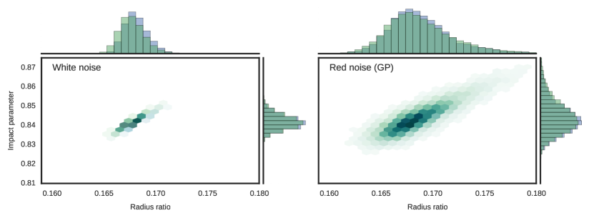
We carry out a broadband (white light) analysis as a consistency test, motivated by the possible issues caused by the TrES-3b’s large impact parameter, and by the need to test whether the spectrum masking has an effect on broadband parameter estimates. TrES-3b has been observed extensively (O’Donovan et al., 2007; Winn et al., 2008; Sozzetti et al., 2009; Gibson et al., 2009; Ballard et al., 2009; Colón et al., 2010; Lee et al., 2011; Turner et al., 2012; Vanko et al., 2013), but many of the analyses have imposed strict priors on the limb darkening, or have considered white noise only. However, the radius ratio, orbital impact parameter and stellar limb darkening are all degenerate, and the transit shape (especially when allowing for red noise) can be explained by a large poorly constrained subvolume of the parameter space.

The broadband modelling is carried out for the light curves with and without spectrum masking, assuming either white or red noise. The red noise is modelled using a Gaussian process with time as the only input parameter (see Sect. 3.4). An exponential kernel producing once-differentiable functions (Roberts et al., 2013; Rasmussen & Williams, 2006) was chosen over the often-used squared exponential (SE) kernel (producing smooth infinitely-differentiable functions) and the slightly more complex Matérn kernel since it was observed to reproduce the noise characteristics better than the SE kernel, but without the additional hyperparameter of a Matérn kernel. We marginalise over the two GP hyperparameters, the length scale and output scale.

The parameter estimation for all cases starts with a parameter vector population that fills uniformly the prior space. An initial differential evolution (DE) optimisation is used to clump the population close to the global posterior maximum, after which MCMC sampling is carried out using emcee. The sampler is run for 10 000 iterations, which yields 9000 independent posterior samples (using a population size of 100, thinning factor of 100, and burn-in period of 1000 iterations, where the thinning factor and burn-in period have been chosen by studying the chain population.)

4.2 Results

The observed light curve, conditional model distribution (for the red noise model) and the residuals are shown in Fig. 7 and the joint posterior distributions for the radius ratio and impact parameter in Fig. 8. The broadband analysis results agree with all the previous TrES-3b analyses, but we will not report the numerical estimates here. Simultaneous multicolour transit modelling described in the next section alleviates the degeneracies between the parameters, and we will adopt the narrow-band analysis results as our final parameter estimates. No significant discrepancies were identified between the masked and unmasked results.

5 Transmission spectroscopy

5.1 Overview

The transmission spectroscopy is carried out for masked and unmasked light curves and three approaches to modelling noise, and follows closely the broadband analysis. The main difference is the need to use a larger parameter vector population (due to high model dimensionality), and special care is needed to ensure that the sampler has converged to sample the true posterior distribution. An initial population of 300 (white noise) or 400 (red noise) parameter vectors is clumped around the global posterior maximum using the DE algorithm, and the population is then used to initialise the MCMC sampler. The MCMC sampling was carried out repeatedly over 15 000 iterations, each run starting from the last iteration of the previous run, until the per-run parameter medians were stable (did not show significant trends compared to the parameter vector population scatter) over the run. The mean autocorrelation lengths were estimated from the MCMC chains, and a thinning factor of 100 was used to ensure that the samples are not significantly correlated.

The red noise model uses GPs similarly to the broadband analysis. Now, however, we do not marginalise over the GP hyperparameters, but fix them to values optimised before the MCMC run (against the residuals from the white-noise run). We tested whether this affects the parameter estimates with a short MCMC run with free GP hyperparameters, but did not find any significant differences.

5.2 Results

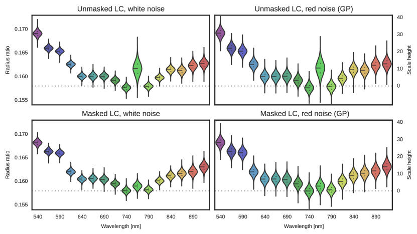
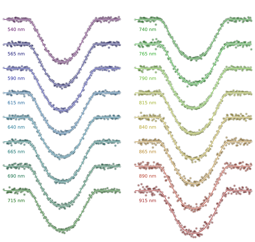
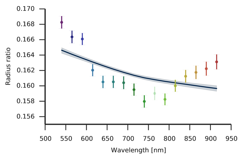
We report the wavelength-independent parameters in Table 3, and show the derived transmission spectra for the 16 narrow-band light curves spanning 530 nm to 930 nm in 25 nm bins in Fig. 9, and the narrow-band light curves (with spectrum masking) and the model in Fig. 10. Shown radius ratio estimates are relative to the average radius ratio. The absolute radius ratio estimates include an uncertainty in the average radius ratio, which will be a major factor in the uncertainty of the per-passband radius ratio estimates. In transmission spectroscopy we are interested in the relative changes between the passbands, and the uncertainty in the average radius ratio is not of interest. The estimates shown here have been corrected for this absolute shift by dividing the radius ratios of each MCMC sample with their average, and then multiplying the relative radius ratios with the total posterior sample mean (0.162). We omit the results from the divide-by-white analysis. The parameter estimates from it are close to the white noise results, only with slightly reduced uncertainties.

The transmission spectrum from the unmasked light curves features a steep increase in radius towards the blue end of the spectrum, and a single peak near 775 nm. The increase towards the blue corresponds to $\sim$30 atmospheric scale heights, which is more than can be realistically expected from Rayleigh scattering (we assume planetary equilibrium temperature of 1620 K and log g of 3.45.) The 767 nm bin that includes the K I resonance doublet also stands out. However, the bin also covers a strong telluric O₂ absorption band, as was shown in Figs. 4 and 5, and spectrum masking completely removes this signal.

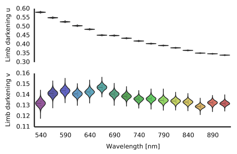
The estimated quadratic limb darkening coefficients are shown in Fig. 11. The posterior estimates are dominated by the likelihood from the stellar limb darkening profiles, since the nearly grazing orbit makes limb darkening poorly constrained by the photometry.

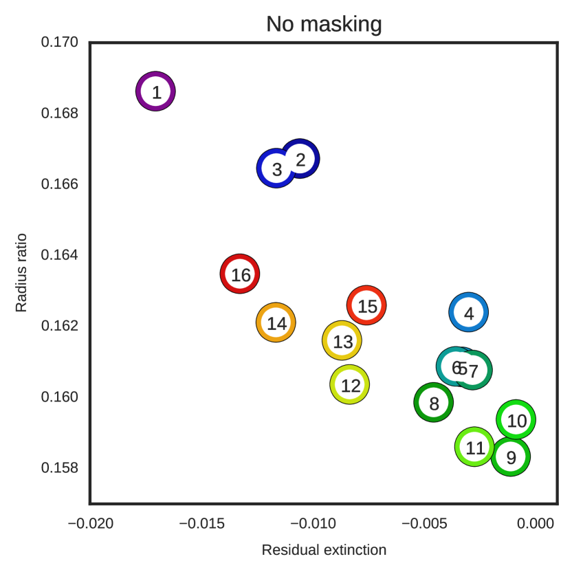
Finally, Fig. 12 shows the narrow-band radius ratios as a function of residual extinction coefficient estimates. The residual extinction coefficients model the atmospheric extinction that is not corrected by dividing the TrES-3b light curves with the comparison star light curves due to different stellar types (that is, the spectra of the two stars are different.) The two parameters are correlated (with a correlation coefficient of -0.83), but it is difficult to assess whether the correlation implies causation. Rayleigh scattering in the Earth’s atmosphere leads to stronger extinction in blue, and a similar scattering mechanism in the Planet’s atmosphere could in theory be behind the observed increase in the radius ratio.

Table 3: Final parameter estimates from the narrow-band analysis.

Parameter	Unit	Value
Transit centre	[MJD]	56846.10945$\quad\pm\;$	4$\times$10-5
Stellar density	[$\mathrm{g\,cm^{-3}}$ ]	2.370$\quad\pm\;$	3.4$\times$10-2
Impact parameter		0.844$\quad\pm\;$	4$\times$10-3
Mean radius ratio		0.162$\quad\pm\;$	1$\times$10-3

Figure 9: TrES-3b transmission spectrum assuming white noise (left) or red time-correlated noise (right) for 25 nm spectral bins covering 530 nm to 930 nm. The potassium doublet lines are at 766.5 nm and 769.9 nm

Figure 10: Observed spectrophotometry with spectrum masking (points) and the fitted model for the 25 nm spectral bins. We have subtracted the GP prediction mean from the observed datapoints and divided by the baseline model for visualisation purposes. A version without the subtraction of the GP prediction mean can be found from the supporting IPython notebook.

Figure 11: Quadratic limb darkening coefficients $u$ and $v$ for the 25 nm spectral bins covering 530 nm to 930 nm. Note that the y-axis scale is different for $u$ and $v$.

Figure 12: Narrow-band radius ratios as a function of residual extinction. The numbers indicate the passband, starting from the shortest wavelength.

5.3 Rayleigh-like signal

The TrES-3b’s radius ratio increases rapidly from 645 nm towards bluer passbands. This signal is similar to what could be expected from Rayleigh scattering, but its amplitude, about 30 atmospheric scale heights assuming planetary equilibrium temperature of 1620 K, is significantly larger than expected from theoretical considerations. The amplitude in scale heights would decrease were the temperature of the observed atmospheric layer to be significantly higher than the planetary equilibrium temperature, and we address this in the end of Sect. 5.3.

The planet’s atmosphere is not the only factor affecting the transmission spectrum, but other sources can have a wavelength-dependent effect on the radius ratio estimates. Especially, systematic errors in the limb darkening models, unocculted star spots, occulted plages, and contamination from an unresolved source can all lead to colour-dependent signals in the radius ratio estimate. Here we first study the effects from each of these one by one, and then combine them into a toy-model to test whether Rayleigh scattering combined with unocculted spots and unaccounted-for contamination could explain the spectrum.

Rayleigh scattering with a constant cloud-deck

Considering only Rayleigh scattering, the slope for the planetary radius is

$$\frac{\mathrm{d}R_{\rm p}}{\mathrm{d}\ln\lambda}=\frac{\alpha Tk_{\mathrm{B}}}{\mu g}=\alpha H,$$ (12)

where $\alpha=-4$, $H$ is the atmospheric scale-heigh, $T$ is the effective temperature, $k_{\mathrm{B}}$ is the Boltzmann constant, $\mu$ is the mean molecular weight of the scatterer, and $g$ is the planet’s surface gravity. The equation for the slope in planet-star radius ratio is now

$$\frac{\mathrm{d}k}{\mathrm{d}\ln\lambda}=\frac{\alpha H}{R_{\star}},$$ (13)

from where we get a simple model for the radius ratio

$$k=\frac{\alpha H}{R_{\star}}\ln\lambda+C,$$ (14)

where $C$ is a constant. If we choose $C$ so that the Rayleigh-scattering $k$ intercepts the constant cloud deck at $k_{0}$ for the wavelength $\lambda_{0}$, we get

$$C=k_{0}-\frac{4H}{R_{\star}}\ln\lambda_{0},$$ (15)

and the toy-model becomes

$$k_{\mathrm{real}}=\max\left(k_{0}-\frac{4H}{R_{\star}}\left(\ln\lambda+\ln\lambda_{0}\right),k_{0}\right).$$ (16)

Adopting $T_{\mathrm{eq}}=1623\pm 26$ K and $\log g_{\mathrm{p}}=3.45\pm 0.02$ from Torres et al. (2008), and $\mu$ as 2.3 time the proton mass, we obtain a normal prior $H\sim N(\text{mean}=205\leavevmode\nobreak\ \mathrm{km},\text{std}=16\leavevmode\nobreak\ \mathrm{km})$.

Effects from unocculted spots

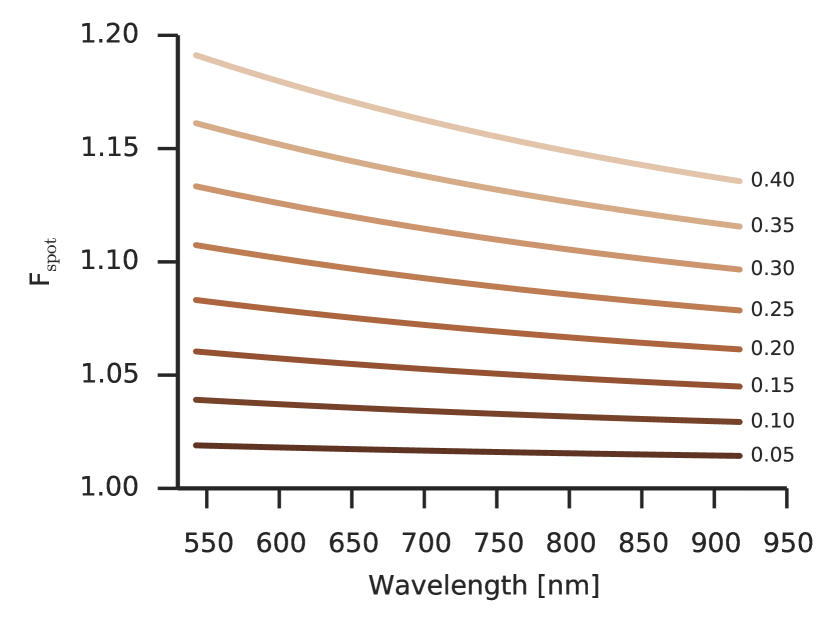
The presence of unocculted star spots can produce an increase in the observed transit depth (and radius ratio) towards blue wavelengths (occulted spots would have their effect also, but they could be distinguished from the photometry). The observed radius ratio, $k_{\mathrm{obs}}$, in the presence of unocculted spots can be expressed as

$$k_{\mathrm{obs}}=k_{\mathrm{real}}\sqrt{\frac{1}{1-fA_{\lambda}}},\qquad A_{\lambda}=1-\frac{P(\lambda,T_{\star}-\Delta T_{\mathrm{s}})}{P(\lambda,T_{\star})},$$ (17)

where $k_{\mathrm{real}}$ the true geometrical radius ratio, $f$ the spot filling factor, and $A_{\lambda}$ the wavelength-dependent contrast ratio, $P$ is the Planck’s law, $\Delta T_{\mathrm{s}}$ is the difference between the spot temperature and effective stellar temperature and $T_{\star}$ is the effective stellar temperature (see Ballerini et al., 2012, for an in-depth treatise).

As shown in Fig. 13, the colour-dependent effect from unocculted spots on $k_{\mathrm{real}}$ for realistic $\Delta T_{\star}$ is nearly linear in visible light, and cannot reproduce the observed signal alone. However, variations in the star spot coverage may explain part of the discrepancy between our average radius ratio estimate and the previous, smaller, estimates.

Figure 13: The effect from unocculted spots on the observed radius ratio as a function of wavelength for $k_{\mathrm{real}}=0.165$, $\Delta T_{\mathrm{s}}=1200$ K, and filling ratios from 0.05 to 0.40. Unocculted spots always increase the observed radius ratio.

Effects from contamination

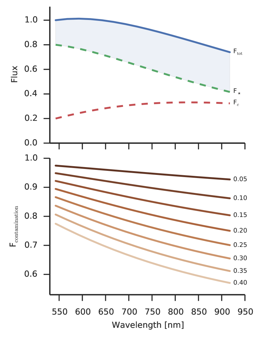
Contamination from an unresolved nearby star falling inside the photometry aperture will also lead to wavelength-dependent effects on the observed radius ratio and transit shape (Tingley, 2004). The observed radius ratio, $k_{\mathrm{obs}}$, is related to the real radius ratio, $k_{\mathrm{real}}$, and wavelength-dependent contamination $c_{\lambda}$ as

$$k_{\mathrm{obs}}=k_{\mathrm{real}}\sqrt{1-c_{\lambda}},$$ (18)

where the contamination factor is the fraction of the contaminant flux from the total observed flux. If we approximate the stellar spectrum with a black body, we get

$$c_{\lambda}=\frac{c_{0}P_{N}(\lambda,T_{\mathrm{c}})}{c_{0}P_{N}(\lambda,T_{\star})+(1-c_{0})P_{N}(\lambda,T_{\mathrm{c}})},$$ (19)

where $P_{N}$ is the Planck’s law normalised to a reference wavelength, $\lambda_{0}$ (that is $P_{N}(\lambda_{0},T)=1$), $T_{\mathrm{c}}$ is the contaminant temperature, $T_{\star}$ is the effective stellar temperature, and $c_{0}$ is the contamination factor for the reference wavelength. The effects form contamination are illustrated in Fig. 14

Figure 14: The effect from third-light contamination on the observed radius ratio. The upper panel depicts the contamination (with an exaggerated situation) as light-blue filled region, with a 3500 K contaminant contributing 20% of the total flux at 545 nm. The solid blue line shows the total flux, the upper dashed line the target flux, and the lower dashed line the contaminating flux. The lower panel shows the wavelength-dependent effect from contamination for a 3500 K contaminant and contamination factor (at 545 nm) varying from 0.05 to 0.40. Contamination always decreases the observed radius ratio, but the exact behaviour depends on the temperature difference between the host star and the contaminant.

Combined model

Combining the effects from Rayleigh scattering, a constant cloud deck, unocculted spots, and possible third-light contamination, we obtain

$$k_{\mathrm{obs}}=\max\left(k_{0}-\frac{4H}{R_{\star}}\left(\ln\lambda+\ln\lambda_{0}\right),k_{0}\right)\sqrt{\frac{1-c_{\lambda}}{1-fA_{\lambda}}},$$ (20)

which is now a function of fractional spot coverage, spot temperature difference, effective temperature of the contaminating star, and the contamination factor for a given reference wavelength.

We carry out an MCMC analysis with a uniform prior on the temperature of the observed atmospheric layer, ranging from the equilibrium temperature to four times the equilibrium temperature, and show the results in Fig. 15. Rayleigh scattering is not able to explain the observed slope, even with the largest possible contributions from unocculted spots and contamination.

Finally, we carry out the analysis with an uninformative prior on atmospheric temperature to obtain an estimate for the temperature that would be required to explain the slope. We obtain a temperature estimate $T\sim 50\,000$ K.

Figure 15: Narrow-band radius ratios and the conditional model distribution for a toy-model that includes Rayleigh scattering, flux contamination, and unocculted spots.

5.4 Systematic errors from limb darkening

The stellar limb darkening is one of the main factors affecting the radius ratio estimates, especially with grazing orbits. Our approach uses the PHOENIX-generated limb darkening profiles as input information, and if the code were to feature systematic deviations from the reality (for example, exaggerated limb darkening towards blue), this would directly affect the $\theta_{\mathrm{k}}$ estimates.

We tested whether the $\theta_{\mathrm{k}}$ difference of 0.01 between the 542.5 nm and 642.5 nm centred passbands (1st and 5th, starting from the bluest) could be explained by systematic errors in limb darkening by first generating a transit light curve corresponding to other passband, and then fitting a transit model to this with free limb darkening coefficients and $\theta_{\mathrm{k}}$ set to the other passband value.

The 542.5 nm light curve can also be explained with $\theta_{\mathrm{k}}=0.175$ and $u=-0.27$ and $v=0.98$. This leads to negligible limb darkening, and is unrealistic at best. The 642.5 nm light curve can be explained with $\theta_{\mathrm{k}}=0.185$ and $u=1.1$ and $v=-0.4$. This would mean that all the redwards limb darkening models would significantly underestimate limb darkening.

For the limb darkening to increase the transit depth when moving towards bluer wavelengths (for a grazing orbit), the overall strength of limb darkening would need to decrease with decreasing wavelength (that is, the limb brightness must increase).

We also carry out a parameter estimation run with a constant radius ratio and impact parameter (both constrained with an informative prior), and limb darkening and the baseline as the only passband-dependent factors. The model fails to reproduce the variations in radius ratio.

6 Conclusions

We have carried out a transmission spectroscopy analysis for TrES-3b, finding initially a strong Rayleigh-like increase in the radius ratio towards the blue end of the spectrum, and a Potassium-like feature near 760 nm. Detailed analysis showed that the Potassium-like feature is due to telluric O₂ absorption, but the origin of the bluewards signal is still unknown (although the correlation with the residual extinction coefficient included into the model suggests that it is not a real feature.) We have included possible flux contamination and unocculted spots into a simple toy model testing how much of the radius ratio variation could be explained by these effects, but note that they fail to explain more than a minor fraction of any wavelength dependent signal.

It is clear that more observations are required to test whether the Rayleigh-like signal is a real atmospheric feature. Current results do not justify a detailed atmospheric modelling. However, if the strong bluewards signal is corroborated by additional observations – transmission spectroscopy or wide-band photometry – more serious modelling is called for to investigate any possible physical processes behind it. Also, transit observations in the NIR, where limb darkening is weaker, will be useful to further constrain TrES-3b’s impact parameter.