Nonparametric estimation of infinitely divisible distributions based on variational analysis on measures

Abstract

The paper develops new methods of non-parametric estimation a compound Poisson distribution. Such a problem arise, in particular, in the inference of a Lévy process recorded at equidistant time intervals. Our key estimator is based on series decomposition of functionals of a measure and relies on the steepest descent technique recently developed in variational analysis of measures. Simulation studies demonstrate applicability domain of our methods and how they positively compare and complement the existing techniques. They are particularly suited for discrete compounding distributions, not necessarily concentrated on a grid nor on the positive or negative semi-axis. They also give good results for continuous distributions provided an appropriate smoothing is used for the obtained atomic measure.

Keywords: Compound Poisson distribution, Lévy process, decompounding, measure optimisation, gradient methods

AMS 2010 Subject Classification. Primary: 62G05, Secondary: 62M05, 65C60

1 Introduction

The paper develops new methods of non-parametric estimation of the distribution of compound Poisson data. Such data naturally arise in the inference of a Lévy process which is a stochastic process $(W_{t})_{t\geq 0}$ with $W_{0}=0$ and time homogeneous independent increments. Its characteristic function necessarily has the form $Ee^{i\theta W_{t}}=e^{t\psi(\theta)}$ with

$$\psi(\theta)=ia\theta-\frac{\sigma^{2}\theta^{2}}{2}+\int(e^{i\theta x}-1-i\theta x\operatorname{{1I}}_{\{|x|<\varepsilon\}})\Lambda(\mathrm{d}x),$$ (1)

where $\varepsilon>0$ is a fixed positive number, $a\in\mathbb{R}$ is a drift parameter, $\sigma^{2}\in[0,\infty)$ is the variance of the Brownian motion component, and the so-called Lévy measure $\Lambda$ satisfying

$$\Lambda(\{0\})=0,\quad\int\min\{1,x^{2}\}\,\Lambda(\mathrm{d}x)<\infty.$$ (2)

Here and below the integrals are taken over the whole $\mathbb{R}$ unless specified otherwise. In a special case with $\sigma=0$ and $\int_{(-\varepsilon,\varepsilon)}|x|\Lambda(\mathrm{d}x)<\infty$, we get a pure jump Lévy process characterised by

$$\psi(\theta)=\int(e^{i\theta x}-1)\Lambda(\mathrm{d}x),$$ (3)

or equivalently,

$$\psi(\theta)=ia\theta+\int(e^{i\theta x}-1-i\theta x\operatorname{{1I}}_{|x|<\varepsilon})\Lambda(\mathrm{d}x),\quad a=\int_{(-\varepsilon,\varepsilon)}x\Lambda(\mathrm{d}x).$$

In an even more restrictive case with a finite total mass $\|\Lambda\|:=\Lambda(\mathbb{R})$, the Lévy process becomes a compound Poisson process with times of jumps being a Poisson process with intensity $\|\Lambda\|$, and the jump sizes being independent random variables with distribution $\|\Lambda\|^{-1}\Lambda(dx)$. Details can be found, for instance, in Sato (1999).

Suppose the Lévy process is observed at regularly spaced times producing a random vector $(W_{0},W_{h},W_{2h},\ldots,W_{nh})$ for some time step $h>0$. The consecutive increments $X_{i}=W_{ih}-W_{(i-1)h}$ then form a vector $(X_{1},\ldots X_{n})$ of independent random variables having a common infinitely divisible distribution with the characteristic function $\varphi(\theta)=e^{h\psi(\theta)}$, and thus can be used to estimate the distributional triplet $(a,\sigma,\Lambda)$ of the process. Such inference problem naturally arises in in financial mathematics Cont and Tankov (2003), queueing theory Asmussen (2008), insurance Mikosch (2009) and in many other situations, where Lévy processes are used.

By the Lévy-Itô representation theorem Sato (1999), every Lévy process is a superposition of a Brownian motion with drift and a square integrable pure jump martingale. The latter can be further decomposed into a pure jump martingale with the jumps not exceeding in absolute value a positive constant $\varepsilon$ and a compound Poisson process with jumps $\varepsilon$ or above. In practice, only a finite increment sample $(X_{1},\dotsc,X_{n})$ is available, so there is no way to distinguish between the small jumps and the Brownian continuous part. Therefore one usually chooses a threshold level $\varepsilon>0$ and attributes all the small jumps to the Brownian component, while the large jumps are attributed to the compound Poisson process component (see, e.g. Asmussen and Rosińsky (2001) for an account of subtleties involved).

Provided an estimation of the continuous and the small jump part is done, it remains to estimate the part of the Lévy measure outside of the interval $(-\varepsilon,\varepsilon)$. Since this corresponds to the compound Poisson case, estimation of such $\Lambda$ is usually called decompounding which is the main object of study in this paper.

Previously developed methods include discrete decompounding approach based on the inversion of Panjer recursions as proposed in Buchmann and Grübel (2003). Comte et al. (2014), Duval (2013) and van Es et al. (2007) studied the continuous decompounding problem when the measure $\Lambda$ is assumed to have a density. They apply Fourier inversion in combination with kernel smoothing techniques for estimating an unknown density of the Lévy measure. In contrast, we do not distinguish between discrete and continuous $\Lambda$ in that our algorithms based on direct optimisation of functionals of a measure work for both situations on a discretised phase space of $\Lambda$. However, if one sees many small atoms appearing in the solution which fill a thin grid, this may indicate that the true measure is absolutely continuous and some kind of smoothing should yield its density.

Specifically, we propose a combination of two non-parametric methods for estimation of the Lévy measure which we call Characteristic Function Fitting (ChF) and Convolution Fitting (CoF). ChF deals with a general class of Lévy processes, while CoF more specifically targets the pure jump Lévy process characterised by (3).

The most straightforward approach is to use the moments fitting, see Feuerverger and McDunnough (1981a) and Carrasco and Florens (2000), or the empirical distribution function

$$\hat{F}_{n}(x)=\frac{1}{n}\sum_{k=1}^{n}\operatorname{{1I}}_{\{X_{k}\leq x\}}$$

to infer about the triplet $(a,\sigma,\Lambda)$. Estimates can be obtained by maximising the likelihood ratio (see, e.g. Quin and Lawless (1994)) or by minimising some measure of proximity between $F(x)$ and $\hat{F}_{n}(x)$, where the dependence on $(a,\sigma,\Lambda)$ comes through $F$ via the inversion formula of the characteristic function:

$$F(x)-F(x-0)=\frac{1}{2\pi}\lim_{y\to\infty}\int_{-y}^{y}\exp\{h\psi(\theta)-i\theta x\}\mathrm{d}\theta.$$

For the estimation, the characteristic function in the integral above is replaced by the empirical characteristic function:

$$\hat{\varphi}_{n}(\theta)=\frac{1}{n}\sum_{k=1}^{n}e^{i\theta X_{k}}.$$

Algorithms based on the inversion of the empirical characteristic function and on the relation between its derivatives were proposed in Watteel and Kulperger (2003). For a comparison between different estimation methods, see a recent survey Sueishi and Nishiyama (2005). Note that inversion of the empirical characteristic function, in contrast to the inversion of its theoretical counterpart, generally leads to a complex valued measure which needs to be dealt with.

Instead, equipped with the new theoretical and numeric optimisation methods developed recently for functionals of measures (see Molchanov and Zuyev (2002) and the references therein), we use the empirical characteristic function directly: the ChF estimator for the compounding measure $\Lambda$ or, more generally, of the whole triplet $(a,\sigma,\Lambda)$ may be obtained by minimisation of the loss functional

$$L_{\mathrm{ChF}}(a,\sigma,\Lambda)=\int|e^{h\psi(\theta)}-\hat{\varphi}_{n}(\theta)|^{2}\omega(\theta)\mathrm{d}\theta,$$ (4)

where $\psi(\theta)\equiv\psi(\theta;a,\sigma,\Lambda)$ is given by (1) and $\omega(\theta)$ is a weight function. Typically $\omega(\theta)$ is a positive constant for $\theta\in[\theta_{1},\theta_{2}]$ and zero otherwise, but it can also be chosen to grow as $\theta\to 0$, this would emphasise a better agreement with the estimated distribution for smaller jumps.

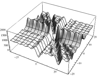
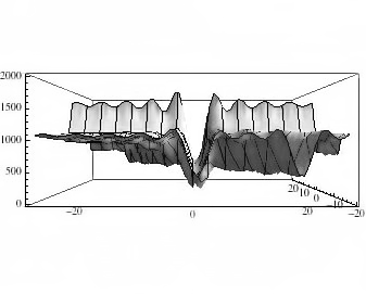
Parametric inference procedures based on the empirical characteristic function has been known for some time, see, e.g., Feuerverger and McDunnough (1981b) and the references therein. Our main contribution is that we compute explicitly the derivative of the loss functional (4) with respect to the measure $\Lambda$ and perform the steepest descent directly on the cone of non-negative measures to a local minimiser. It must be noted that, as a simple example reveal, the functionals based on the empirical characteristic function usually have a very irregular structure, see Figure 1. As a result, the steepest descent often fails to attend the global optimal solution, unless the starting point of the optimisation procedure is carefully chosen.

Figure 1: Illustration of intrinsic difficulties faced by any characteristic function fitting procedure. Suppose one knows the data are coming from a shifted Poisson distribution (i.e. $\sigma=0$ and the Lévy measure has the form $\Lambda=x\delta_{1}$). Assume now a big data sample is actually coming from a Poisson $\mathsf{Po}(1)$ distribution so that $\hat{\varphi}_{n}$ in (4) is very close to $\exp\{e^{i\theta}-1)\}$. Plotted are the values of (4) with shift parameter $-20\leq a\leq 20$ and $0\leq x\leq 20$. It is seen that any optimisation algorithm would have difficulties converging to the global minimum $a=0,\ x=1$ even in this simple two parameter case.

In contrast, the proposed CoF estimation method is not using the empirical characteristic function and is based on Theorem 2 below which presents the convolution

$$F^{*2}(x)=\int F(u)F(y-u)du$$

as a functional of $\Lambda$. It has an explicit form of an infinite Taylor series in direct products of $\Lambda$, but truncating it to only the first $k$ terms we build a loss function $L_{\mathrm{CoF}}^{(k)}$ by comparing two estimates of $F^{*2}$: the one based on the truncated series and the other being the empirical convolution $F^{2*}_{n}$. CoF is able to produce nearly optimal estimates $\hat{\Lambda}_{k}$ when large values of $k$ are taken, but this also drastically increases the computation time.

A practical combination of these methods recommended by this paper is to find $\hat{\Lambda}_{k}$ using CoF with a low value of $k$, and then apply ChF with $\hat{\Lambda}_{k}$ as the starting value. The estimate for such a two-step procedure will be denoted by $\tilde{\Lambda}_{k}$ in the sequel.

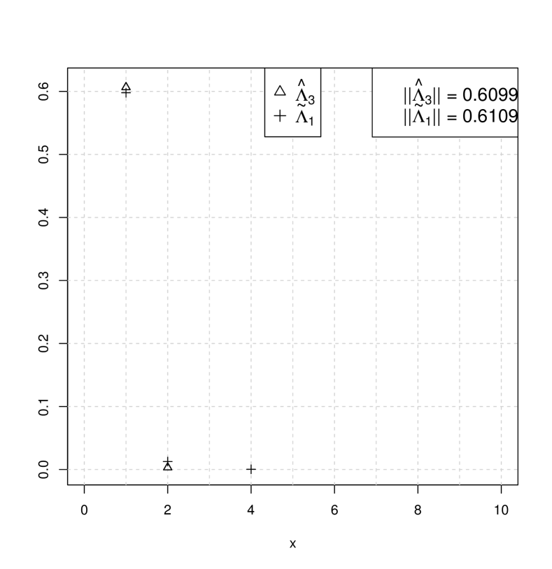
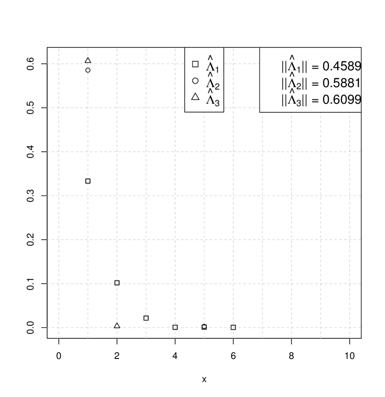
To give an early impression of our approach, let us demonstrate the performance of the ChF methods on the famous data by Ladislaus Bortkiewicz who collected the numbers of Prussian soldiers killed by a horse kick in 10 cavalry corps over a 20 years period Bortkiewicz (1898). The counts 0, 1, 2, 3, and 4 were observed 109, 65, 22, 3 and 1 times, with 0.6100 deaths per year and cavalry unit. The author argues that the data are Poisson distributed which corresponds to the measure $\Lambda$ concentrated on the point $\{1\}$ (only jumps of size 1) and the mass being the parameter of the Poisson distribution which is then estimated by the sample mean 0.61. Figure 2 on its left panel presents the estimated Lévy measures for the cutoff values $k=1,2,3$ when using CoF method. For the values of $k=1,2$, the result is a measure having many atoms. This is explained by the fact that the accuracy of the convolution approximation is not enough for this data, but $k=3$ already results in a measure $\hat{\Lambda}_{3}$ essentially concentrated at $\{1\}$ thus supporting the Poisson model with parameter $\|\hat{\Lambda}_{3}\|=0.6098$. In Section 6 we return to this example and explain why the choice of $k=3$ is reasonable.We observed that the convergence of the ChF method depends critically on the choice of the initial measure, especially on its total mass. However, the proposed combination of CoF followed by ChF demonstrates (the right plot) that this two-step (faster) procedure results in the estimate $\tilde{\Lambda}_{1}$ which is as good as $\hat{\Lambda}_{3}$.

The rest of the paper has the following structure. Section 2 introduces the theoretical basis of our approach – a constraint optimisation technique in the space of measures. In Section 3 we perform analytic calculations of the gradient of the loss functionals needed for the implementation of ChF. Section 4 develops the necessary ingredients for the CoF method and proves the main analytical result of the paper, Theorem 2. In Section 5 we give some details on the implementation of our algorithms in R-language. Section 6 contains a broad range of simulation results illustrating performance of our algorithms. We conclude by Section 7, where we summarise our approach and give some practical recommendations.

Figure 2: The Bortkiewicz horse kick data. Left panel: comparison of CoF estimates for $k=1,2,3$. Right panel: comparison of the estimate by CoF with $k=3$ and a combination of CoF with $k=1$ followed by ChF.

2 Optimisation in the space of measures.

In this section we briefly present the main ingredients of the constrained optimisation of functionals of a measure. Further details can be found in Molchanov and Zuyev (2000a) and Molchanov and Zuyev (2000b).

In this paper we are dealing with measures defined on the Borel subsets of $\mathbb{R}$. Recall that any signed measure $\eta$ can be represented in terms of its Jordan decomposition: $\eta=\eta^{+}+\eta^{-}$, where $\eta^{+}$ and $\eta^{-}$ are orthogonal non-negative measures. The total variation norm is then defined to be $\|\eta\|=\eta^{+}(\mathbb{R})+\eta^{-}(\mathbb{R})$. Denote by $\mathbb{M}$ and $\mathbb{M}_{+}$ the class of signed, respectively, non-negative measures with a finite total variation. The set $\mathbb{M}$ then becomes a Banach space with sum and multiplication by real numbers defined set-wise: $(\eta_{1}+\eta_{2})(B):=\eta_{1}(B)+\eta_{2}(B)$ and $(t\eta)(B):=t\eta(B)$ for any Borel set $B$ and any real $t$. The set $\mathbb{M}_{+}$ is a pointed cone in $\mathbb{M}$ meaning that the zero measure is in $\mathbb{M}_{+}$ and that $\mu_{1}+\mu_{2}\in\mathbb{M}_{+}$ and $t\mu\in\mathbb{M}_{+}$ as long as $\mu_{1},\mu_{2},\mu\in\mathbb{M}_{+}$ and $t\geq 0$.

A functional $G:\mathbb{M}\mapsto\mathbb{R}$ is called Fréchet or strongly differentiable at $\eta\in\mathbb{M}$ if there exists a bounded linear operator (a differential) $DG(\eta)[\cdot]:\ \mathbb{M}\mapsto\mathbb{R}$ such that

$$G(\eta+\nu)-G(\eta)=DG(\eta)[\nu]+o(\|\nu\|)\ \nu\in\mathbb{M}.$$ (5)

If for a given $\eta\in\mathbb{M}$ there exists a bounded function $\nabla G(\,\cdot\,;\eta)\,:\,\mathbb{R}\to\mathbb{R}$ such that

$$DG(\eta)[\nu]=\int\nabla G(x;\eta)\,\nu(\mathrm{d}x)\ \text{for all}\ \nu\in\mathbb{M},$$

then such $\nabla G(x;\eta)$ is called the gradient function for $G$ at $\eta$. Typically, and it is the case for the functionals of measure we consider here, the gradient function does exist so that the differentials do have an integral form.

For example, an integral of a bounded function $G(\eta)=\int f(x)\eta(dx)$ is already a bounded linear functional of $\eta$ so that $\nabla G(x;\eta)=f(x)$ for any $\eta$. More generally, for a composition $G(\eta)=v(\int f(x)\eta(\mathrm{d}x))$, where $v$ is a differentiable function, the gradient function can be obtained by the Chain rule:

$$\nabla G(x;\eta)=v^{\prime}\Bigl{(}\int f(y)\,\eta(\mathrm{d}y)\Bigr{)}\,f(x).$$ (6)

The functional $G$ for this example is strongly differentiable if both functions $v^{\prime}$ and $f$ are bounded.

The estimation methods we develop here are based on minimisation of various loss functions over the class of possible Lévy measures with a finite mass. Specifically, we consider minimisation of a strongly differentiable functional

$$L(\Lambda)\to\min\quad\text{subject to}\ \Lambda\in\mathbb{M}_{+},\ H(\Lambda)\in C,$$ (7)

where the last constraint singles out the set of Lévy measures, i.e. the measures satisfying (2). This corresponds to taking $C=\{0\}\times\mathbb{R}$ being a cone in $\mathbb{R}^{2}$ and

$$H(\Lambda)=\Bigl{(}\Lambda(\{0\}),\int\min\{1,x^{2}\}\,\Lambda(\mathrm{d}x)\Bigr{)}.$$ (8)

Theorem 1.

Suppose $L\,:\,\mathbb{M}\to\mathbb{R}$ is strongly differentiable at a positive finite measure $\Lambda$ satisfying (2) and possess a gradient function $\nabla L(x;\Lambda)$. If such $\Lambda$ provides a local minimum of $L$ over $\mathbb{M}_{+}\cap H^{-1}(C)$, then

$$\begin{cases}\nabla L(x;\Lambda)\geq 0\quad\text{for all}\ x\in\mathbb{R}\setminus\{0\},\\ \nabla L(x;\Lambda)=0\quad\Lambda-a.e.\\ \end{cases}$$ (9)

Proof.

First-order necessary criteria for constrained optimisation in a Banach space can be derived in terms of tangent cones. Let $\mathbb{A}$ be a subset of $\mathbb{M}$ and $\eta\in\mathbb{A}$. The tangent cone to $\mathbb{A}$ at $\eta$ is the following subset of $\mathbb{M}$:

$$\mathbb{T}_{\mathbb{A}}(\eta)=\liminf_{t\downarrow 0}t^{-1}(\mathbb{A}-\eta).$$

Recall that the $\liminf_{n}A_{n}$ for a family of subsets $(A_{n})$ in a normed space is the set of the limits of all converging sequences $\{a_{n}\}$ such that $a_{n}\in A_{n}$ for all $n$. Equivalently, $\mathbb{T}_{\mathbb{A}}(\eta)$ is the closure of the set of such $\nu\in\mathbb{M}$ for which there exists an $\varepsilon=\varepsilon(\nu)>0$ such that $\eta+t\nu\in\mathbb{A}$ for all $0\leq t\leq\varepsilon$.

By the definition of the tangent cone, if $\eta$ is a point of minimum of a strongly differentiable function $G$ over a set $\mathbb{A}$ then one must have

$$DG(\eta)[\nu]\geq 0\quad\text{for all}\ \nu\in\mathbb{T}_{\mathbb{A}}(\eta).$$ (10)

Indeed, assume that there exists $\nu\in\mathbb{T}_{\mathbb{A}}(\eta)$ such that $DG(\eta)[\nu]:=-\varepsilon<0$. Then there is a sequence of positive numbers $t_{n}\downarrow 0$ and a sequence $\eta_{n}\in\mathbb{A}$ such that $\nu=\lim_{n}t_{n}^{-1}(\eta_{n}-\eta)$ implying $\eta_{n}\to\eta$ because $\|\eta-\eta_{n}\|=t_{n}(1+o(1))\|\nu\|\to 0$. Since any bounded linear operator is continuous, we also have

$$DG(\eta)[\nu]=DG(\eta)[\lim_{n}t_{n}^{-1}(\eta_{n}-\eta)]=\lim_{n}t_{n}^{-1}DG(\eta)[\eta_{n}-\eta]=-\varepsilon.$$

Furthermore, by (5),

$$DG(\eta)[\eta_{n}-\eta]=G(\eta_{n})-G(\eta)+o(\|\eta-\eta_{n}\|)=G(\eta_{n})-G(\eta)+o(t_{n}),$$

thus

$$G(\eta_{n})-G(\eta)=-t_{n}\varepsilon(1+o(1))<-t_{n}\varepsilon/2$$

for all sufficiently small $t_{n}$. Thus in any ball of $\eta$ there is a $\eta_{n}\in\mathbb{A}$ such that $G(\eta_{n})<G(\eta)$ so that $\eta$ is not a point of a local minimum of $G$ over $\mathbb{A}$.

Next step is to find a sufficiently rich class of measures belonging to the tangent cone to the set $\mathbb{L}:=\mathbb{M}_{+}\cap H^{-1}(C)$ of all possible Lévy measures. For this, notice that for any $\Lambda\in\mathbb{L}$, the Dirac measure $\delta_{x}$ belongs to $\mathbb{T}_{\mathbb{L}}(\Lambda)$ since $\Lambda+t\delta_{x}\in\mathbb{L}$ for any $t\geq 0$ as soon as $x\neq 0$. Similarly, given any Borel $B\subset\mathbb{R}$, the negative measure $-\Lambda|_{B}=-\Lambda(\,\cdot\,\cap B)$, which is the restriction of $-\Lambda$ onto $B$, is also in the tangent cone $\mathbb{T}_{\mathbb{L}}(\Lambda)$, because for any $0\leq t\leq 1$ we have $\Lambda-t\Lambda_{B}\in\mathbb{L}$.

Since $\nabla G(x;\Lambda)$ is a gradient function, the necessary condition (10) becomes

$$\int\nabla G(x;\Lambda)\,\nu(\mathrm{d}x)\geq 0\quad\text{for all}\ \nu\in\mathbb{T}_{\mathbb{L}}(\Lambda)$$

and substituting $\nu=\delta_{x}$ above we immediately obtain the inequality in (9). Finally, taking $\nu=-\Lambda_{B}$ yields

$$\int_{B}\nabla G(x;\Lambda)\,\Lambda(\mathrm{d}x)\leq 0.$$

Since this is true for any Borel $B$, then $G(x;\Lambda)\leq 0$ $\Lambda$-almost everywhere which, combined with the previous inequality, gives the second identity in (9).

∎

A rich class of functions of a measure represent the expectation of a functionals of a Poisson process.

Let $\boldsymbol{N}$ be the space of locally finite counting measures $\varphi$ on a Polish space $X$ which will be a subset of an Euclidean space in this paper. Let $\mathcal{N}$ be the smallest $\sigma$-algebra which makes all the mappings $\varphi\mapsto\varphi(B)\in\mathbb{Z}_{+}$ for $\varphi\in\boldsymbol{N}$ and compact sets $B$ measurable. A Poisson point process with the intensity measure $\mu$ is a measurable mapping $\Pi$ from some probability space into $[\boldsymbol{N},\mathcal{N}]$ such that for any finite family of disjoint compact sets $B_{1},\dotsc,B_{k}$, the random variables $\Pi(B_{1}),\dotsc,\Pi(B_{k})$ are independent and each $\Pi(B_{i})$ following Poisson distribution with parameter $\mu(B_{i})$. We use notation $\Pi\sim\mathrm{PPP}(\mu)$. From the definition, $\operatorname{{\bf E}}\Pi(B)=\mu(B)$, this is why the parameter measure $\mu$ of a Poisson process is indeed the intensity measure of this point process. To emphasise the dependence of the distribution on $\mu$, we write the expectation as $\operatorname{{\bf E}}_{\mu}$ in the sequel.

Consider a measurable function $G\colon\boldsymbol{N}\to\mathbb{R}$ and define the difference operator

$$D_{z}G(\varphi):=G(\varphi+\delta_{z})-G(\varphi),\ \varphi\in\boldsymbol{N}.$$

For the iterations of the difference operator

$$D_{z_{1},\ldots,z_{n}}G=D_{z_{n}}(D_{z_{1},\ldots,z_{n-1}}G),$$

and every tuple of points $(z_{1},\ldots,z_{n})\in X^{n}$, it can be checked that

$$D_{z_{1},\ldots,z_{n}}G(\nu)=\sum_{J\subset\{1,2,\ldots,n\}}(-1)^{n-|J|}G\big{(}\nu+\Sigma_{j\in J}\delta_{z_{j}}\big{)},$$

where $|J|$ stands for the cardinality of $J$. Define

$$T_{\mu}G(z_{1},\ldots,z_{n}):=\operatorname{{\bf E}}_{\mu}D_{z_{1},\ldots,z_{n}}G(\Pi).$$

Suppose that the functional $G$ is such that there exists a constant $c>0$ satisfying

$$|G\big{(}{\Sigma}_{j=1}^{n}\delta_{z_{j}}\big{)}|\leq c^{n}$$

for all $n\geq 1$ and all $(z_{1},\ldots z_{n})$. It was proved in (Molchanov and Zuyev, 2000b, Theorem 2.1) that in the case of finite measures $\mu,\mu^{\prime}$ if then expectation $\operatorname{{\bf E}}_{\mu+\mu^{\prime}}G(\Pi)$ exists then

$$\operatorname{{\bf E}}_{\mu+\mu^{\prime}}G(\Pi)=\operatorname{{\bf E}}_{\mu}G(\Pi)+\sum_{n=1}^{\infty}\frac{1}{n!}\int_{X^{n}}T_{\mu}G(z_{1},\dots,z_{n})\mu^{\prime}(\mathrm{d}z_{1})\ldots\mu^{\prime}(\mathrm{d}z_{n}).$$ (11)

Generalisations of this formula to infinite and signed measures for square integrable functionals can be found in Last (2014). A finite order expansion formula can be obtained by representing the expectation above in the form $\operatorname{{\bf E}}_{\mu+\mu^{\prime}}G(\Pi)=\operatorname{{\bf E}}_{\mu}\operatorname{{\bf E}}_{\mu^{\prime}}[G(\Pi+\Pi^{\prime})\hskip 4.30554pt\rule[-4.30554pt]{0.6458pt}{12.91663pt}\hskip 4.30554pt\Pi]$ where $\Pi$ and $\Pi^{\prime}$ are independent Poisson processes with intensity measures $\mu$ and $\mu^{\prime}$, respectively, and then applying the moment expansion formula by (Błaszczyszyn et al., 1997, Theorem 3.1) to $G(\Pi+\Pi^{\prime})$ viewed as a functional of $\Pi^{\prime}$ with a given $\Pi$. This will give

$$\operatorname{{\bf E}}_{\mu+\mu^{\prime}}G(\Pi)=\operatorname{{\bf E}}_{\mu}G(\Pi)+\sum_{n=1}^{k}\frac{1}{n!}\int_{X^{n}}T_{\mu}G(z_{1},\dots,z_{n})\mu^{\prime}(\mathrm{d}z_{1})\ldots\mu^{\prime}(\mathrm{d}z_{n})\\ +\frac{1}{(k+1)!}\int_{X^{k+1}}T_{\mu+\mu^{\prime}}G(z_{1},\dots,z_{k+1})\mu^{\prime}(\mathrm{d}z_{1})\ldots\mu^{\prime}(\mathrm{d}z_{k+1}).$$ (12)

3 Gradients of ChF loss function

The ChF method of estimating the compounding distribution $\Lambda$ or more generally, the tripplet $(a,\sigma,\Lambda)$ of the infinite divisible distribution, is based on fitting the empirical characteristic function. The corresponding loss function $L_{\mathrm{ChF}}$ is given by (4). It is everywhere differentiable in the usual sense with respect to the parameters $a,\sigma$ and in Fréchet sense with respect to measure $\Lambda$. Aiming at the steepest descent gradient method for obtaining its minimum, we compute in this section the gradients of $L_{\mathrm{ChF}}$ in terms of the following functions

$$q_{1}(\theta,x) :=\cos(\theta x)-1,\quad Q_{1}(\theta,\Lambda):=\int q_{1}(\theta,x)\Lambda(\mathrm{d}x);$$

$$q_{2}(\theta,x) :=\sin(\theta x)-\theta x\operatorname{{1I}}_{\{|x|<\varepsilon\}},\quad Q_{2}(\theta,a,\Lambda):=a\theta+\int q_{2}(\theta,x)\Lambda(\mathrm{d}x).$$

Using this notation, the real and imaginary parts of an infinitely divisible distributions characteristic function $\varphi=\varphi_{1}+i\varphi_{2}$ can be written down as

$$\varphi_{1}(\theta;a,\sigma,\Lambda) =e^{h\{Q_{1}(\theta,\Lambda)-\sigma^{2}\theta^{2}/2\}}\cos\{hQ_{2}(\theta,a,\Lambda)\},$$

$$\varphi_{2}(\theta;a,\sigma,\Lambda) =e^{h\{Q_{1}(\theta,\Lambda)-\sigma^{2}\theta^{2}/2\}}\sin\{hQ_{2}(\theta,a,\Lambda)\}.$$

After noticing that $\hat{\varphi}_{n}=\hat{\varphi}_{n,1}+i\hat{\varphi}_{n,2}$, with

$$\hat{\varphi}_{n,1}(\theta)=\frac{1}{n}\sum_{j=1}^{n}\cos(\theta X_{j}),\qquad\hat{\varphi}_{n,2}(\theta)=\frac{1}{n}\sum_{j=1}^{n}\sin(\theta X_{j}),$$

the loss functional $L_{\mathrm{ChF}}$ can be written as

$$L_{\mathrm{ChF}}(a,\sigma,\Lambda)=\int\big{\{}\varphi_{1}(\theta;a,\sigma,\Lambda)-\hat{\varphi}_{n,1}(\theta)\big{\}}^{2}\omega(\theta)\mathrm{d}\theta+\int\big{\{}\varphi_{2}(\theta;a,\sigma,\Lambda)-\hat{\varphi}_{n,2}(\theta)\big{\}}^{2}\omega(\theta)\mathrm{d}\theta.$$

From this representation, the following tree sets of formulae are obtained in a straightforward way.

1. The partial derivative of the loss functional with respect to $a$ is equal to

   $${\partial\over\partial a}L_{\mathrm{ChF}}(\theta;a,\sigma,\Lambda) =2\int\{\varphi_{1}(\theta;a,\sigma,\Lambda)-\hat{\varphi}_{n,1}(\theta)\}{\partial\over\partial a}\varphi_{1}(\theta;a,\sigma,\Lambda)\omega(\theta)\mathrm{d}\theta$$

   $$\quad+2\int\{\varphi_{2}(\theta;a,\sigma,\Lambda)-\hat{\varphi}_{n,2}(\theta)\}{\partial\over\partial a}\varphi_{2}(\theta;a,\sigma,\Lambda)\omega(\theta)\mathrm{d}\theta,$$

   where

   $${\partial\over\partial a}\varphi_{1}(\theta;a,\sigma,\Lambda) =-h\theta e^{h\{Q_{1}(\theta,\Lambda)-\sigma^{2}\theta^{2}/2\}}\sin\{hQ_{2}(\theta,a,\Lambda)\},$$

   $${\partial\over\partial a}\varphi_{2}(\theta;a,\sigma,\Lambda) =h\theta e^{h\{Q_{1}(\theta,\Lambda)-\sigma^{2}\theta^{2}/2\}}\cos\{hQ_{2}(\theta,a,\Lambda)\}.$$

2. The partial derivative of the loss functional with respect to $\sigma$ is equal to

   $${\partial\over\partial\sigma}L_{\mathrm{ChF}}(\theta;a,\sigma,\Lambda) =2\int\{\varphi_{1}(\theta;a,\sigma,\Lambda)-\hat{\varphi}_{n,1}(\theta)\}{\partial\over\partial\sigma}\varphi_{1}(\theta;a,\sigma,\Lambda)\omega(\theta)\mathrm{d}\theta$$

   $$\quad+2\int\{\varphi_{2}(\theta;a,\sigma,\Lambda)-\hat{\varphi}_{n,2}(\theta)\}{\partial\over\partial\sigma}\varphi_{2}(\theta;a,\sigma,\Lambda)\omega(\theta)\mathrm{d}\theta,$$

   where

   $${\partial\over\partial\sigma}\varphi_{1}(\theta;a,\sigma,\Lambda) =-h\sigma\theta^{2}e^{h\{Q_{1}(\theta,\Lambda)-\sigma^{2}\theta^{2}/2\}}\cos\{hQ_{2}(\theta,a,\Lambda)\},$$

   $${\partial\over\partial\sigma}\varphi_{2}(\theta;a,\sigma,\Lambda) =-h\sigma\theta^{2}e^{h\{Q_{1}(\theta,\Lambda)-\sigma^{2}\theta^{2}/2\}}\sin\{hQ_{2}(\theta,a,\Lambda)\}.$$

3. Expression for the gradient function corresponding to the Fréchet derivative with respect to the measure $\Lambda$ is obtained using the Chain rule (6):

   $$\nabla L_{\mathrm{ChF}}(x;\Lambda) =2\int\{\varphi_{1}(\theta;a,\sigma,\Lambda)-\hat{\varphi}_{n,1}(\theta)]\}\nabla\varphi_{1}(\theta)[x,\Lambda]\omega(\theta)\mathrm{d}\theta$$

   $$\quad+2\int\{\varphi_{2}(\theta;a,\sigma,\Lambda)-\hat{\varphi}_{n,2}(\theta)\}\nabla\varphi_{2}(\theta)[x,\Lambda]\omega(\theta)\mathrm{d}\theta,$$

   where the gradients of $\varphi_{i}(\theta):=\varphi_{i}(\theta;a,\sigma,\Lambda)$, $i=1,2$, with respect to the measure $\Lambda$ are given by

   $$\nabla\varphi_{1}(\theta)(x;\Lambda) =he^{h\{Q_{1}(\theta,\Lambda)-\sigma^{2}\theta^{2}/2\}}\big{\{}\cos\big{(}hQ_{2}(\theta,a,\Lambda)\big{)}q_{1}(\theta,x)-\sin\big{(}hQ_{2}(\theta,a,\Lambda)\big{)}q_{2}(\theta,x)\big{\}},$$

   $$\nabla\varphi_{2}(\theta)(x;\Lambda) =he^{h\{Q_{1}(\theta,\Lambda)-\sigma^{2}\theta^{2}/2\}}\big{\{}\sin\big{(}hQ_{2}(\theta,a,\Lambda)\big{)}q_{1}(\theta,x)+\cos\big{(}hQ_{2}(\theta,a,\Lambda)\big{)}q_{2}(\theta,x)\big{\}}.$$

4 Description of the CoF method

As it was alluded in the Introduction, the CoF method uses a representation of the convolution as a function of the compounding measure. We now formulate the main theoretical result of the paper on which the CoF method is based.

Theorem 2.

Let $W_{t}$ be a pure jump Lévy process characterised by (3) and $F(y)=F_{h}(y)$ be the cumulative distribution function of $W_{h}$. Then one has

$$\begin{split}F^{*2}(y)&=F(y)+\sum_{n=1}^{\infty}\frac{h^{n}}{n!}\int_{\mathbb{R}^{n}}U_{x_{1},\ldots,x_{n}}F(y)\Lambda(\mathrm{d}x_{1})\ldots\Lambda(\mathrm{d}x_{n}),\end{split}$$ (13)

where $U_{x_{1}}F(y)=F(y-x)-F(x)$ and

$$U_{x_{1},\ldots,x_{n}}F(y):=U_{x_{n}}(U_{x_{1},\ldots,x_{n-1}}F(y))=\sum_{J\subset\{1,2,\ldots,n\}}(-1)^{i-|J|}F(y-\Sigma_{j\in J}x_{j}).$$ (14)

The sum above is taken over all the subsets $J$ of $\{1,2,\ldots,n\}$ including the empty set.

Proof.

To prove the theorem, we use a coupling of $W_{t}$ with a Poisson process $\Pi$ on $\mathbb{R}_{+}\times\mathbb{R}$ driven by the intensity measure $\mu=\ell\times\Lambda$, where $\ell$ is the Lebesgue measure on $\mathbb{R}_{+}$. For each realisation $\Pi=\Sigma_{j}\delta_{z_{j}}$ with $z_{j}=(t_{j},x_{j})$, denote by $\Pi_{t}$ the restriction of $\Pi$ onto $[0,t]\times\mathbb{R}$. Then, the Lévy process can be represented as

$$W_{t}=\Sigma_{(t_{j},x_{j})\in\Pi_{t}}x_{j}=\int_{0}^{t}\int_{\mathbb{R}}x\Pi(\mathrm{d}s\,\mathrm{d}x).$$

For a fixed arbitrary $y\in\mathbb{R}$ and a point configuration $\varphi=\Sigma_{j}\delta_{(t_{i},x_{j})}$, consider a functional $G_{y}$ defined by

$$G_{y}(\varphi)=\operatorname{{1I}}\Bigl{\{}\sum_{(t_{j},x_{j})\in\varphi}x_{j}\leq y\Bigr{\}}$$

and notice that for any $z=(t,x)$,

$$G_{y}(\varphi+\delta_{z})=\operatorname{{1I}}\Bigl{\{}\sum_{(t_{j},x_{j})\in\varphi}x_{j}\leq y-x\Bigr{\}}=G_{y-x}(\varphi).$$ (15)

Clearly, the cumulative distribution function of $W_{h}$ can be expressed as an expectation

$$F(y)=\mathbf{P}_{\mu}\Big{\{}\sum_{(t_{j},x_{j})\in\Pi_{h}}x_{j}\leq y\Big{\}}=\operatorname{{\bf E}}_{\mu}G_{y}(\Pi_{h}).$$

Let $\mu^{\prime}=[0,h]\times\Lambda$ and $\mu^{\prime\prime}=[h,2h]\times\Lambda$. Then

$$\operatorname{{\bf E}}_{\mu^{\prime}+\mu^{\prime\prime}}G_{y}(\Pi)=\mathbf{P}\{W_{2h}\leq y\}=\mathbf{P}\{W_{h}+W_{h}^{\prime\prime}\leq y\}=F^{*2}(y),$$

where $W_{h}^{\prime\prime}=W_{2h}-W_{h}$. Observe also that by iteration of (15),

$$T_{\mu^{\prime}}G_{y}(z_{1},\ldots,z_{n}) =\operatorname{{\bf E}}_{\mu^{\prime}}D_{z_{1},\ldots,z_{n}}G_{y}(\Pi)=\sum_{J\subset\{1,2,\ldots,n\}}(-1)^{n-|J|}\operatorname{{\bf E}}_{\mu^{\prime}}G_{y}\big{(}\Pi+\Sigma_{j\in J}\delta_{z_{j}}\big{)}$$

$$=\sum_{J\subset\{1,2,\ldots,n\}}(-1)^{n-|J|}F(y-\Sigma_{j\in J}x_{j})=U_{x_{1},\ldots,x_{n}}F(y).$$

It remains now to apply expansion (11) to complete the proof:

$$F^{*2}(y) =\operatorname{{\bf E}}_{\mu^{\prime}+\mu^{\prime\prime}}G_{y}(\Pi)$$

$$=F(y)+\sum_{n=1}^{\infty}\frac{1}{n!}\int_{(\mathbb{R}_{+}\times\mathbb{R})^{n}}U_{x_{1},\ldots,x_{n}}F(y)\,\mu^{\prime\prime}(\mathrm{d}t_{1}\,\mathrm{d}x_{1})\ldots\mu^{\prime\prime}(\mathrm{d}t_{n}\,\mathrm{d}x_{n})$$

$$=F(y)+\sum_{n=1}^{\infty}\frac{h^{n}}{n!}\int_{\mathbb{R}^{n}}U_{x_{1},\ldots,x_{n}}F(y)\,\Lambda(\mathrm{d}x_{1})\ldots\Lambda(\mathrm{d}x_{n}).$$

∎

The empirical convolution of a sample $(X_{1},\dotsc,X_{n})$,

$$\hat{F}_{n}^{*2}(y):=\frac{1}{\binom{n}{2}}\sum_{1\leq i<j\leq n}\operatorname{{1I}}\{X_{i}+X_{j}\leq y\}.$$ (16)

is an unbiased and consistent estimator of $F^{*2}(x)$, see Frees (1986).

The CoF-method looks for a finite measure $\Lambda$ that minimises the following loss function

$$L_{\mathrm{CoF}}^{(k)}(\Lambda)=\int\Big{\{}\hat{F}(y)+\sum_{i=1}^{k}\frac{h^{i}}{i!}\int_{\mathbb{R}^{i}}U_{x_{1},\ldots,x_{i}}\hat{F}_{n}(y)\Lambda(\mathrm{d}x_{1})\ldots\Lambda(\mathrm{d}x_{i})-\hat{F}_{n}^{*2}(y)\Big{\}}^{2}\omega(y)\mathrm{d}y.$$ (17)

The infinite sum in (13) is truncated to $k$ terms in (17) for computational reasons. The error introduced by the truncation can be accurately estimated by bounding the remainder term in the finite expansion formula (12). Alternatively, turning to (13) and using $0\leq F(y)\leq 1$, we obtain that $|U_{x_{1},\ldots,x_{i}}F(y)|\leq 2^{i-1}$ for all $i=1,2,\dots$, yielding

$$\Big{|}\frac{h^{k+1}}{(k+1)!}\int_{\mathbb{R}^{k+1}}U_{x_{1},\ldots,x_{k+1}}F(y)\Lambda(\mathrm{d}x_{1})\ldots\Lambda(\mathrm{d}x_{k+1})\Big{|}\leq\frac{1}{2}\sum_{i=k+1}^{\infty}\frac{(2h\|\Lambda\|)^{i}}{i!}.$$

Notice that the upper bound corresponds to a half the distribution tail $\mathbf{P}\{Z\geq k+1\}$ of a Poisson random variable, say $Z\sim\mathsf{Po}(2h\|\Lambda\|)$. Thus, to have a good estimate with this method, one should either calibrate the time step $h$ (if the data are coming from the discretisation of a Lévy process trajectory) or to use higher $k$ to make the remainder term small enough. For instance, for the horse kick data considered in Introduction 1, $h=1$ and $\|\Lambda\|=0.61$. The resulting error bounds for $k=1,2,3$ are 0.172, 0.062 and 0.017, respectively, which shows that $k=3$ is rather adequate cutoff for this data. Since $h\|\Lambda\|$ is the mean number of jumps in the strip $[0,h]\times\mathbb{R}$, in practice one should aim to choose $h$ so that to have only a few jumps with high probability. If, on the contrary, the number of jumps is high, their sum by the Central Limit theorem would be close to the limiting law which, in the case of a finite variance of jumps, is Normal and so depends on the first two moments only and not on the entire compounding distribution. Therefore an effective estimation of $\Lambda/\|\Lambda\|$ is impossible in this case, see Duval (2014) for a related discussion.

As with the ChF method, the CoF algorithm relies on the steepest descent approach. The needed gradient function has the form

$$\nabla L_{\mathrm{CoF}}^{(k)}(x;\Lambda)$$

$$=2h\int\Big{\{}\hat{F}_{n}(y)+\sum_{i=1}^{k}\frac{h^{i}}{i!}\int_{\mathbb{R}^{i}}U_{x_{1},\ldots,x_{i}}\hat{F}_{n}(y)\Lambda(\mathrm{d}x_{1})\ldots\Lambda(\mathrm{d}x_{i})-\hat{F}_{n}^{*2}(y)\Big{\}}\Gamma(y,x,\Lambda)\omega(y)\mathrm{d}y,$$

where

$$\Gamma(y,x,\Lambda)=\sum_{j=0}^{k-1}\frac{h^{j}}{j!}\int_{\mathbb{R}^{j}}(U_{x,x_{1},\ldots,x_{j}}\hat{F}_{n})(y)\Lambda(\mathrm{d}x_{1})\ldots\Lambda(\mathrm{d}x_{j}).$$

This formula follows from the Chain rule (6) and the equality

$$\nabla\Big{(}\sum_{j=1}^{k}\frac{h^{j}}{j!}\int_{\mathbb{R}^{j}} (U_{x_{1},\ldots,x_{j}}\hat{F}_{n})(y)\Lambda(\mathrm{d}x_{1})\ldots\Lambda(\mathrm{d}x_{j})\Big{)}(x;\Lambda)$$

$$=h\sum_{j=0}^{k-1}\frac{h^{j}}{j!}\int_{\mathbb{R}^{j}}(U_{x,x_{1},\ldots,x_{j}}\hat{F}_{n})(y)\Lambda(\mathrm{d}x_{1})\ldots\Lambda(\mathrm{d}x_{j}).$$

To justify the last identity, it suffices to see that for any integrable symmetric function $u(x_{1},\ldots,x_{j})$ of $j\geq 1$ variables,

$$\nabla\Big{(}\int_{\mathbb{R}^{j}}u(x_{1},\ldots,x_{j}) \Lambda(\mathrm{d}x_{1})\ldots\Lambda(\mathrm{d}x_{j})\Big{)}(x;\Lambda)$$

$$=j\int_{\mathbb{R}^{j-1}}u(x,x_{1},\ldots,x_{j-1})\Lambda(\mathrm{d}x_{1})\ldots\Lambda(\mathrm{d}x_{j-1}),$$

which holds due to

$$\int_{\mathbb{R}^{j}} u(x_{1},\ldots,x_{j})(\Lambda+\nu)(\mathrm{d}x_{1})\ldots(\Lambda+\nu)(\mathrm{d}x_{j})-\int_{\mathbb{R}^{j}}u(x_{1},\ldots,x_{j})\Lambda(\mathrm{d}x_{1})\ldots\Lambda(\mathrm{d}x_{j})$$

$$=\sum_{k=1}^{j}\int_{\mathbb{R}^{j}}u(x_{1},\ldots,x_{j})\Lambda(\mathrm{d}x_{1})\ldots\Lambda(\mathrm{d}x_{k-1})\nu(\mathrm{d}x_{k})\Lambda(\mathrm{d}x_{k+1})\ldots\Lambda(\mathrm{d}x_{j})+o(\|\nu\|)$$

$$=j\int_{\mathbb{R}^{j}}u(x,x_{1},\ldots,x_{j-1})\nu(\mathrm{d}x)\Lambda(\mathrm{d}x_{1})\ldots\Lambda(\mathrm{d}x_{j-1})+o(\|\nu\|).$$

5 Algorithmic implementation of the steepest descent method

In this section we describe the algorithm implementing the gradient descent method, which was used to obtain our simulation results presented in Section 6.

Recall that the principal optimisation problem has the form (7), where the functional $L(\Lambda)$ is minimised over $\Lambda\in\mathbb{M}_{+}$ subject to the constraints on being a Lévy measure. For computational purposes the measure $\Lambda\in\mathbb{M}_{+}$ is replaced by its discrete approximation which has a form of a linear combination $\boldsymbol{\Lambda}=\Sigma_{i=1}^{l}\lambda_{i}\delta_{x_{i}}$ of Dirac measures on a finite regular grid $x_{1},\ldots,x_{l}\in\mathbb{R}$, $x_{i+1}=x_{i}+2\Delta$. Specifically, for a given measure $\Lambda$, the atoms of $\boldsymbol{\Lambda}$ are given by

$$\lambda_{1} :=\Lambda((-\infty,x_{1}+\Delta)),$$

$$\lambda_{i} :=\Lambda([x_{i}-\Delta,x_{i}+\Delta)),\quad\text{for }i=2,\ldots,l-1,$$ (18)

$$\lambda_{l} :=\Lambda([x_{l}-\Delta,\infty)).$$

Clearly, the larger is $l$ and the finer is the grid $\{x_{1},\ldots,x_{l}\}$ the better is approximation, however, at a higher computational cost.

Respectively, the discretised version of the gradient function $\nabla L(x;\Lambda)$ is the vector

$$\boldsymbol{g}=(g_{1},\ldots,g_{l}),\quad g_{i}:=\nabla L(x_{i};\boldsymbol{\Lambda}),\quad i=1,\ldots,l.$$

For example, the cost function $L=L^{(1)}_{\rm CoF}$ with $\omega(y)\equiv 1$ has the gradient

$$\nabla L_{\mathrm{CoF}}^{(1)}(x;\Lambda)=2h\int\Big{\{}\hat{F}_{n}(y)-\hat{F}_{n}^{*2}(y)+\int\hat{F}_{n}(y-z)\Lambda(\mathrm{d}z)\Big{\}}\hat{F}_{n}(y-x)\,\mathrm{d}y.$$

The discretised gradient for this example is the vector $\boldsymbol{g}$ with the components

$$g_{i}=2h\int\Big{\{}\hat{F}_{n}(y)-\hat{F}_{n}^{*2}(y)+\sum_{j=1}^{l}\hat{F}_{n}(y-x_{j})\lambda_{j}\Big{\}}\hat{F}_{n}(y-x_{i})\,\mathrm{d}y,\quad i=1,\dotsc,l.$$ (19)

Our main optimisation algorithm has the following structure:

Algorithm 1 Steepest descent algorithm

1:initial vector $\boldsymbol{\Lambda}$

2:function GoSteep($\boldsymbol{\Lambda}$)

3:     initialise the discretised gradient $\boldsymbol{g}\leftarrow(\nabla L(x_{1};\boldsymbol{\Lambda}),\ldots,\nabla L(x_{l};\boldsymbol{\Lambda}))$

4:     while ( $\min_{i}g_{i}<-\tau_{2}$ or $\max_{\{i\colon\lambda_{i}>\tau_{1}\}}g_{i}>\tau_{2}$ ) do

5:         choose a favourable step size $\varepsilon$ depending on $L$ and $\boldsymbol{\Lambda}$

6:         compute new vector $\boldsymbol{\Lambda}\leftarrow$ MakeStep($\varepsilon$, $\boldsymbol{\Lambda}$, $\boldsymbol{g}$)

7:         compute gradient at the new $\boldsymbol{\Lambda}$: $\boldsymbol{g}\leftarrow(\nabla L(x_{1};\boldsymbol{\Lambda}),\ldots,\nabla L(x_{l};\boldsymbol{\Lambda}))$

8:     end while

9:     return $\boldsymbol{\Lambda}$

10:end function

In the master algorithm description above, the line 3 uses the necessary condition (9) as a test condition for the main cycle. In the computer realisations we usually want to discard the atoms of a negligible size: for this purpose we use a zero-value threshold parameter $\tau_{1}$. We use another threshold parameter $\tau_{2}$ to decide when the coordinates of the gradient vector are sufficiently small. For the examples considered in the next section, we typically used the following values: $\omega\equiv 1$, $\tau_{1}=10^{-2}$ and $\tau_{2}=10^{-6}$. The key MakeStep subroutine, mentioned on line 5, is described below. It calculates the admissible steepest direction $\boldsymbol{\nu}^{*}$ of size $\|\boldsymbol{\nu}^{*}\|\leq\varepsilon$ and returns an updated vector $\boldsymbol{\Lambda}\leftarrow\boldsymbol{\Lambda}+\boldsymbol{\nu}^{*}$.

Algorithm 2 Algorithm for a steepest descent move

1:maximal step size $\varepsilon$, current variable value $\boldsymbol{\Lambda}$ and current gradient value $\boldsymbol{g}$

2:function MakeStep($\varepsilon$, $\boldsymbol{\Lambda}$, $\boldsymbol{g}$)

3:     initialise the optimal step $\boldsymbol{\nu^{*}}\leftarrow\boldsymbol{0}$

4:     initialise the running coordinate $i\leftarrow 0$

5:     initialise the total mass available $E\leftarrow\varepsilon$

6:     while  (($E>0$) and ($i\leq l$))  do

7:         if  $g_{i}>|g_{l}|$  then

8:              $\nu_{i}^{*}\leftarrow\max(-\lambda_{i},-E)$

9:              $E\leftarrow E-\nu_{i}^{*}$

10:         else

11:              $\nu_{l}^{*}\leftarrow E$

12:              $E\leftarrow 0$

13:         end if

14:         $i\leftarrow i+1$

15:     end while

16:     return $\boldsymbol{\Lambda}+\boldsymbol{\nu^{*}}$

17:end function

The MakeStep subroutine looks for a vector $\boldsymbol{\nu}^{*}$ which minimises the linear form $\sum_{i=1}^{l}g_{i}\nu_{i}$ appearing in the Taylor expansion

$$L(\boldsymbol{\Lambda}+\boldsymbol{\nu})-L(\boldsymbol{\Lambda})=\sum_{i=1}^{l}g_{i}\nu_{i}+o(|\boldsymbol{\nu}|).$$

This minimisation is subject to the following linear constraints

$$\sum_{i=1}^{l}|\nu_{i}|\leq\varepsilon,$$

$$\nu_{i}\geq-\lambda_{i},\quad i=1,\ldots,l.$$

The just described linear programming task has a straightforward solution given below.

For simplicity we assume that $g_{1}\geq\ldots\geq g_{l}$. Note that this ordering can always be achieved by a permutation of the components of the vector $\boldsymbol{g}$ and respectively, $\boldsymbol{\Lambda}$. Assume also that the total mass of $\boldsymbol{\Lambda}$ is bigger than the stepsize $\varepsilon$. Define two indices

$$i_{g}=\max\{i\colon g_{i}\geq|g_{l}|\},\quad\text{and}\quad i_{\varepsilon}=\max\{i\colon\sum_{j=1}^{i-1}\lambda_{j}<\varepsilon\},\quad\varepsilon>0.$$

If $i_{\varepsilon}\leq i_{g}$, then the coordinates of $\boldsymbol{\nu}^{*}$ are given by

$$\nu_{i}^{*}:=\left\{\begin{array}[]{ll}-\lambda_{i}&\text{for }i\leq i_{\varepsilon},\\ \sum_{j=1}^{i_{\varepsilon}-1}\lambda_{j}-\varepsilon&\text{for }i=i_{\varepsilon}+1,\\ 0&\text{for }i\geq i_{\varepsilon}+2,\end{array}\right.$$

and if $i_{\varepsilon}>i_{g}$, then

$$\nu_{i}^{*}:=\left\{\begin{array}[]{ll}-\lambda_{i},&\text{for }i\leq i_{g},\\ 0&\text{for }i_{g}<i<l,\\ \varepsilon-\sum_{j=1}^{i_{g}}\lambda_{j}&\text{for }i=l.\end{array}\right.$$

The presented algorithm is realised in the statistical computation environment R (see R Core Team (2015)) in the form of a library mesop which is freely downloadable from one of the authors’ webpage.

6 Simulation results for a discrete Lévy measure

To illustrate the performance of our estimation methods we generated samples of size $n=1000$ for compound Poisson processes driven by different kinds of Lévy measure $\Lambda$. For all examples in this section, we implement three versions of the CoF with $h=1$, $k=1,2,3$ and $\omega\equiv 1$. We also apply ChF using the estimate of CoF with $k=1$. Observe that CoF with $k=1$ can be made particularly fast because here we have a non-negative least squares optimisation problem.

Poisson compounding distribution.

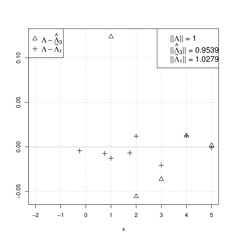
Here we consider the simplest possible Lévy measure $\Lambda(dx)=\delta_{1}(dx)$ which corresponds to a standard Poisson process with parameter 1. Since all the jumps are integer valued and non-negative, it is logical take the non-negative integer grid for possible atom positions of the discretised $\Lambda$. This is the way we have done it for the horse kick data analysis. However, to test the robustness of our methods, we took the grid $\{0,\pm 1/4,\pm 2/4,\pm 3/4,\ldots\}$. As a result the estimated measures might place some mass on non-integer points or even on negative values of $x$ to compensate for inaccurately fitted positive jumps. We have chosen to show on the graphs the discrepancies between the estimated and the true measure. An important indicator of the effectiveness of an estimation is the closeness of the total masses $\|\hat{\Lambda}\|$ and $\|\Lambda\|$. For $\Lambda=\delta_{1}$, the probability to have more than 3 jumps is approximately 0.02, therefore we expect that $k=3$ would give an adequate estimate for this data. Indeed, the left panel of Figure 3 demonstrates that the CoF with $k=3$ is quite effective in detecting the jumps of the Poisson process compared to $k=2$ and especially to $k=1$ which generate large discrepancies both in atom sizes and in the total mass of the obtained measure. Observe also the presence of artefact small atoms at large $x$ and even at some non-integer locations.

The right panel shows that a good alternative to a rather computationally demanding CoF method with $k=3$, is a much faster combined CoF–ChF method when $\hat{\Lambda}_{1}$ measure is used as the initial measure in the ChF algorithm. The resulting measure $\tilde{\Lambda}_{1}$ is almost idetical to $\hat{\Lambda}_{3}$, but also has the total mass closer to the target value 1. The total variation distances between the estimated measure and the theoretical one are 0.435, 0.084 and 0.053 for $k=1,2,3$, respectively. For the combined method it is 0.043 which is the best approximation in the total variation to the original measure.

Figure 3: Simulation results for a Poisson $\mathsf{Po}(1)$ compounding distribution corresponding to $\Lambda$ concentrated at point $1$, with total mass $1$. Left panel: the differences between $\Lambda(\{x\})$ and their estimates $\hat{\Lambda}_{k}(\{x\})$ obtained by CoF with $k=1,2,3$. Zero values of the differences are not plotted. Right panel: comparison of $\hat{\Lambda}_{3}$ with $\tilde{\Lambda}_{1}$ obtained by ChF initiated at $\hat{\Lambda}_{1}$. Notice the drastic change in the vertical axis scale as we go from the left to the right panel.

Compounding distribution with positive and negative jumps.

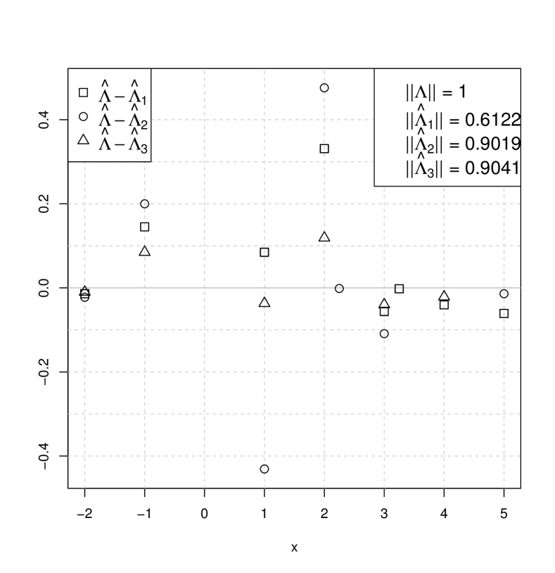
Figure 4 presents the results on a compound Poisson process with jumps of sizes $-1,1,2$ having respective probabilities 0.2, 0.2 and 0.6, so that $\Lambda=0.2\delta_{-1}+0.2\delta_{1}+0.6\delta_{2}$. The overall intensity of the jumps is again $\|\Lambda\|=1$. The presence of negative jumps canceling positive jumps creates an additional difficulty for the estimation task. This phenomenon explains why the approximation obtained with $k=2$ is worse than with $k=1$ and $k=3$: two jumps of sizes +1 and -1 sometimes cancel each other, which is indistinguishable from no jumps case. Moreover, -1 and 2 added together is the same as having a single size 1 jump. The left panel confirms that going from $k=1$ through $k=2$ up to $k=3$ improves the performance of CoF although the computing time increases drastically. The corresponding total variation distances of $\hat{\Lambda}_{k}$ to the theoretical distribution are 0.3669, 0.6268 and 0.1558. The combined method gives the distance 0.0975 and according to the right plot is again a clear winner in this case too. It is also much faster.

Figure 4: Simulation results for $\Lambda=0.2\delta_{-1}+0.2\delta_{1}+0.6\delta_{2}$. Left panel: the differences between $\Lambda(\{x\})$ and their estimates $\hat{\Lambda}_{k}(\{x\})$ obtained by CoF with $k=1,2,3$. Right panel: comparison of $\hat{\Lambda}_{3}$ with $\tilde{\Lambda}_{1}$

Figure 5: Simulation results for a shifted Poisson distribution $\Lambda(\{x\})={e^{-1}/(x-1)!}$ for $x=1,2,\ldots$. Left panel: the differences between $\Lambda(\{x\})$ and their estimates $\hat{\Lambda}_{k}(\{x\})$ obtained by CoF with $k=1,2,3$. Right panel: comparison of $\hat{\Lambda}_{3}$ with $\tilde{\Lambda}_{1}$ obtained by ChF initiated at $\hat{\Lambda}_{1}$.

Unbounded compounding distribution.

On Figure 5 we present the simulation results for a discrete measure $\Lambda$ having an infinite support $\mathbb{N}$. For the computation, we limit the support range for the measures in question to the interval $x\in[-2,5]$. As the left panel reveals, also in this case the CoF method with $k=3$ gives a better approximation than $k=1$ or $k=2$ (the total variation distances to the theoretical distribution is 0.1150 compared to 0.3256 and 0.9235, respectively) and the combined faster method gives even better estimate with $d_{\mathrm{TV}}(\tilde{\Lambda}_{1},\Lambda)=0.0386$. Interestingly, $k=2$ was the worst in terms of the total variation distance. We suspect that the ’pairing effect’ may be responsible: the jumps are better fitted with a single integer valued variable rather than the sum of two. The algorithm may also got stuck in a local minimum producing small atoms at non-integer positions.

Finally, we present simulation results for two cases of continuously distributed jumps. The continuous measures are replaced by their discretised versions given by (18). In the examples below the grid size is $\Delta=0.25$.

Continuous non-negative compounding distribution.

Figure 6 summarises our simulation results for the compound Poisson distribution with the jump sizes following the exponential $\mathsf{Exp}(1)$ distribution. The left plot shows that also in this case the accuracy of approximation increases with $k$. Observe that the total variation distance $d_{\mathrm{TV}}(\hat{\Lambda}_{3},\boldsymbol{\Lambda})=0.0985$ is comparable with the discretisation error: $d_{\mathrm{TV}}(\Lambda,\boldsymbol{\Lambda})=0.075$. A Gaussian kernel smoothed version of $\hat{\Lambda}_{3}$ is presented at the right plot of Figure 6. The visible discrepancy for small values of $x$ is explained by the fact that there were no sufficient number of really small jumps in the simulated sample to give the algorithm sufficient grounds to put more mass around 0. Interestingly, the combined algorithm produced a measure with a smaller (compared to $\hat{\Lambda}_{3}$) value of the $L_{\mathrm{ChF}}$, but a larger total variation distance from $\boldsymbol{\Lambda}$. Optimisation in the space of measures usually tends to produce atomic measures since these are boundary points of the typical constraint sets in $\mathbb{M}$. Indeed, $\tilde{\Lambda}_{1}$ has smaller number of atoms than $\boldsymbol{\Lambda}$ does and still it better approximates the empirical characteristic function of the sample. It shows that the case of optimisation in the class of absolutely continuous measures should be analysed differently by characterising their tangent cones and deriving the corresponding steepest descent methods. Additional conditions on the density must also be imposed, like Lipschitz kind of conditions, to make the feasible set closed in the corresponding measure topology.

Figure 6: Simulation results for a compound Poisson process with jump intensity 1 and jump sizes having an exponential distribution with parameter $1$. Left plot: obtained measures for various algorithms, the right plot: the theoretical exponential density and the smoothed version of $\tilde{\Lambda}_{1}$ measure.

Gaussian compounding distribution.

Figure 7 takes up the important example of compound Poisson processes with Gaussian jumps. Once again, the estimates $\hat{\Lambda}_{k}$ improve as $k$ increases, and the combined method gives an estimate similar to $\hat{\Lambda}_{3}$.

Figure 7: Left plot: Estimated compounding measure for a simulated sample with jump sizes having the standard Normal distribution with mean 0.5 and variance 0.25. Right plot: the theoretical Gaussian density and the smoothed version of $\hat{\Lambda}_{3}$ measure.

7 Discussion

In this paper we proposed and analysed new algorithms based on the characteristic function fitting (ChF) and convoluted cumulative distribution function fitting (CoF) for non-parametric inference of the compounding measure of a pure-jump Lévy process. The algorithms are based on the recently developed variational analysis of functionals of measures and the corresponding steepest descent methods for constraint optimisation on the cone of measures. CoF methods are capable of producing very accurate estimates, but at the expense of growing computational complexity. The ChF method critically depends on the initial approximation measure due to highly irregular behaviour of the objective function. We have shown that the problems of convergence of the ChF algorithms can often be effectively overcome by choosing the sample measure (discretised to the grid) as the initial approximation measure. However, a better alternative, as we demonstrated in the paper, is to use the measure obtained by the simplest ($k=1$) CoF algorithm. This combined CoF–ChF algorithm is fast and in majority of cases produces a measure which is closest in the total variation to the measure under estimation and thus this is our method of choice.

The practical experience we gained during various tests allows us to conclude that the suggested methods are especially well suited for estimation of discrete jump size distributions. They work well even with jumps that take both positive and negative values not necessarily belonging to a regular lattice, demonstrating a clear advantage over the existing methods, see Buchmann and Grübel (2003), Buchmann and Grübel (2004). Use of our algorithms for continuous compounding distributions require more trial and error in choosing the right discretisation grid and smoothing procedures to produce good results which should be then compared or complemented to the direct methods of the density estimation like in van Es et al. (2007), Watteel and Kulperger (2003).

References

• Sato (1999) K. Sato. Lévy Processes and Infinitely Divisible Distributions (Cambridge Studies in Advanced Mathematics). Cambridge University Press, 1st edition, November 1999. ISBN 0521553024. URL http://www.amazon.com/exec/obidos/redirect?tag=citeulike07-20&path=ASIN/0521553024.
• Cont and Tankov (2003) R. Cont and P. Tankov. Financial Modelling with Jump Processes. Chapman & Hall/CRC, 2003.
• Asmussen (2008) S. Asmussen. Applied Probability and Queues. Stochastic Modelling and Applied Probability. Springer New York, 2008. ISBN 9780387215259. URL https://books.google.se/books?id=c4_xBwAAQBAJ.
• Mikosch (2009) T. Mikosch. Non-Life Insurance Mathematics: An Introduction with the Poisson Process. Universitext. Springer, 2009. ISBN 9783540882336. URL https://books.google.se/books?id=yOgoraGQhGEC.
• Asmussen and Rosińsky (2001) S. Asmussen and J. Rosińsky. Approximations of small jumps of lévy process with a vew towards simulation. J. Appl. Prob., 38:482–493, 2001.
• Buchmann and Grübel (2003) B. Buchmann and R. Grübel. Decompounding: an estimation problem for poisson random sums. Ann. Statist., 31(4):1054–1074, 08 2003. doi: 10.1214/aos/1059655905. URL http://dx.doi.org/10.1214/aos/1059655905.
• Comte et al. (2014) F. Comte, C. Duval, and V. Genon-Catalot. Nonparametric density estimation in compound poisson processes using convolution power estimators. Metrika, 77(1):163–183, 2014. URL http://EconPapers.repec.org/RePEc:spr:metrik:v:77:y:2014:i:1:p:163-183.
• Duval (2013) C. Duval. Density estimation for compound poisson processes from discrete data. Stochastic Processes and their Applications, 123(11):3963–3986, 2013. doi: http://dx.doi.org/10.1016/j.spa.2013.06.006. URL http://www.sciencedirect.com/science/article/pii/S0304414913001683.
• van Es et al. (2007) B. van Es, S. Gugushvili, and P. Spreij. A kernel type nonparametric density estimator for decompounding. Bernoulli, 13(3):672–694, 08 2007. doi: 10.3150/07-BEJ6091. URL http://dx.doi.org/10.3150/07-BEJ6091.
• Feuerverger and McDunnough (1981a) A. Feuerverger and P. McDunnough. On some Fourier methods for inference. J. American Stat. Assoc., 76:379–387, 1981a.
• Carrasco and Florens (2000) M. Carrasco and J.P. Florens. Generaliza- tion of gmm to a continuum of moment conditions. Economic Theory, 16:797–834, 2000.
• Quin and Lawless (1994) J. Quin and J. Lawless. Empirical likelihood and general estimating equations. Ann. Statist., 22:300–325, 1994.
• Watteel and Kulperger (2003) R.N. Watteel and R.J. Kulperger. Nonpatrametric estimation of the canonical measure for infinitely divisible distributions. J. Statist. Comp. Simul., 73(7):525–542, 2003.
• Sueishi and Nishiyama (2005) N. Sueishi and Y. Nishiyama. Estimation of Lévy processes in mathematical finance: A comparative study. In A. Zerger and R.M. Argent, editors, MODSIM 2005 International Congress on Modelling and Simulation., pages 953–959. Modelling and Simulation Society of Australia and New Zealand, December 2005. URL http://http://www.mssanz.org.au/modsim05/papers/sueishi.pdf.
• Molchanov and Zuyev (2002) I. Molchanov and S. Zuyev. Steepest descent algorithms in a space of measures. Statistics and Computing, 12:115 – 123, 2002.
• Feuerverger and McDunnough (1981b) A. Feuerverger and P. McDunnough. On the efficiency of empirical characteristic function procedures. J. Royal. Stat. Soc., Ser. B, 43:20–27, 1981b.
• Bortkiewicz (1898) L. Bortkiewicz. Das gesetz der kleinen zahlen. Monatshefte für Mathematik und Physik, 9(1):A39–A41, 1898.
• Molchanov and Zuyev (2000a) I. Molchanov and S. Zuyev. Tangent sets in the space of measures: With applications to variational analysis. Journal of Mathematical Analysis and Applications, 249(2):539 – 552, 2000a. doi: http://dx.doi.org/10.1006/jmaa.2000.6906. URL http://www.sciencedirect.com/science/article/pii/S0022247X00969063.
• Molchanov and Zuyev (2000b) I. Molchanov and S. Zuyev. Variational analysis of functionals of poisson processes. Mathematics of Operations Research, 25(3):485–508, 2000b. doi: 10.1287/moor.25.3.485.12217. URL http://dx.doi.org/10.1287/moor.25.3.485.12217.
• Last (2014) G. Last. Perturbation analysis of poisson processes. Bernoulli, 20(2):486–513, 05 2014. doi: 10.3150/12-BEJ494. URL http://dx.doi.org/10.3150/12-BEJ494.
• Błaszczyszyn et al. (1997) B. Błaszczyszyn, E. Merzbach, and V. Schmidt. A note on expansion for functionals of spatial marked point processes. Statist. Probab. Lett., 36(3):299–306, 1997. doi: 10.1016/S0167-7152(97)00076-X. URL http://dx.doi.org/10.1016/S0167-7152(97)00076-X.
• Frees (1986) E.W. Frees. Nonparametric renewal function estimation. Ann. Statist., 14(4):1366–1378, 12 1986. doi: 10.1214/aos/1176350163. URL http://dx.doi.org/10.1214/aos/1176350163.
• Duval (2014) C. Duval. When is it no longer possible to estimate a compound poisson process? Electron. J. Statist., 8(1):274–301, 2014. doi: 10.1214/14-EJS885. URL http://dx.doi.org/10.1214/14-EJS885.
• R Core Team (2015) R Core Team. R: A Language and Environment for Statistical Computing. R Foundation for Statistical Computing, Vienna, Austria, 2015. URL https://www.R-project.org.
• Buchmann and Grübel (2004) B. Buchmann and R. Grübel. Decompounding poisson random sums: Recursively truncated estimates in the discrete case. Annals of the Institute of Statistical Mathematics, 56(4):743–756, 2004. ISSN 0020-3157. doi: 10.1007/BF02506487. URL http://dx.doi.org/10.1007/BF02506487.