Phenomenological investigation of a quantum gravity extension of inflation with the Starobinsky potential

Abstract

We investigate the pre-inflationary dynamics of inflation with the Starobinsky potential, favored by recent data from the Planck mission, using techniques developed to study cosmological perturbations on quantum spacetimes in the framework of loop quantum cosmology. We find that for a large part of the initial data, inflation compatible with observations occurs. There exists a subset of this initial data that leads to quantum gravity signatures that are potentially observable. Interestingly, despite the different inflationary dynamics, these quantum gravity corrections to the powerspectra are similar to those obtained for inflation with a quadratic potential, including suppression of power at large scales. Furthermore, for super horizon modes the tensor modes show deviations from the standard inflationary paradigm that are unique to the Starobinsky potential and could be important for non-Gaussian modulation and tensor fossils.

I Introduction

The paradigm of cosmic inflation is the most accepted one that explains the origin of the anisotropy observed in the cosmic microwave background (CMB). The inflationary phase of accelerated expansion stretches tiny primordial quantum inhomogeneities to large scale perturbations which in turn seed the large scale structure observed today guth ; albrecht ; linde ; lindechaotic ; liddlelyth ; mukhanov ; weinberg . This is a remarkable accomplishment of cosmology. Inflation is often modeled by a scalar field with a self-interacting potential that gives rise to a slow-roll phase during which the energy density of the matter field remains nearly constant and the spacetime behaves like a quasi-de Sitter spacetime. However, there is no unique way of obtaining slow-roll inflation. There are numerous inflationary models that give rise to a quasi-de Sitter phase including single field inflation with various potentials, quasi-single field inflation, Dirac-Born-Infeld inflation and multi-field inflation. Fortunately, recent results from the Planck mission planck2013 and WMAP wmap7 are able to rule out various scenarios and favor a few. In particular, the data show that single field inflation with a quadratic potential is moderately disfavored and plateau-like inflationary potentials including the Starobinsky potential are favored. This has led to an increased interest in studying single field inflation with a Starobinsky potential.

However, as shown by Borde, Guth and Vilenkin borde , despite its great success the standard inflationary scenario, which is based on classical general relativity, is past incomplete due to the presence of big bang singularity. This is true for all models of scalar field inflation including the Starobinsky potential. The problem of a big bang singularity is an artifact of using Einstein’s equations all the way to the Planck scale. It is expected that these problems will be resolved by a quantum theory of gravity which will depart from classical general relativity in the deep Planck regime. Several important questions arise for such a theory: Is there a consistent extension of the inflationary scenario all the way to the Planck scale? Will inflation occur naturally, or would one require special fine tuning on the initial conditions to obtain a desired phase of inflation? To answer these questions the fundamental quantum gravity theory, while modifying the Planck scale physics, must be in agreement with classical general relativity (GR) when the spacetime curvature is well below the Planck scale. The theory will have to provide a consistent framework where one can study the evolution of scalar and tensor perturbations. Additionally, the theory should be able to provide natural initial conditions for the quantum perturbations in the deep Planck regime. Will these initial conditions lead to the usual Bunch-Davies state used in the standard inflationary scenario, or are they different? Can there be quantum gravity corrections to the standard power spectra? Modern CMB observations have put strong constraints on various aspects of the scalar and tensor power spectra. Are the predictions from the fundamental quantum gravity theory compatible with these observational data? As was shown in aan2 ; aan3 all these questions can be answered in the framework of loop quantum cosmology (LQC). In this paper we will study the inflationary scenario with a Starobinsky potential in the LQC framework.

Over the past decade, LQC has emerged as a concrete framework to address these issues and study the evolution of both the background and cosmological perturbations all the way to the Planck scale aps2 ; aps3 ; aan2 ; aan3 (for other approaches to studying cosmological perturbations within LQC, see FernandezMendez:2012vi ; Gomar:2015oea ; Barrau:2013ula ; Cailleteau:2011kr ; Barrau:2014maa ; Bojowald:2011aa ; Zhu:2015ata ). Indeed, a key feature of LQC models is the resolution of classical big bang type singularities via a non-singular quantum bounce. Extensive analytical and numerical studies have been carried out to understand the nature of a variety of cosmological models in the quantum gravity regime where the spacetime curvature is Planckian. For example: the flat Friedmann-Lemaître-Robertson-Walker (FLRW) model which we will be focusing on in this paper bojowaldprl01 ; aps2 ; aps3 ; acs ; ps09 , open and closed FLRW models apsv ; warsaw_closed ; singhk-1 , the flat FLRW model in the presence of cosmological constants bp ; kp1 ; ap , various homogeneous and anisotropic models awe2 ; awe3 ; we1 ; b1madrid1 ; b1madrid2 and their generalizations to include inhomogeneities wemadrid1 ; bmp1 ; bmp2 (see as1 for an up-to-date review). Occurrence of the quantum bounce is a robust prediction of LQC in all these models which remains independent of the choice of initial conditions and energy conditions acs ; ps09 ; dgs2 ; dgms ; cyclic .

It is now natural to raise questions discussed above in the context of LQC. Extensive analytical and numerical studies performed in aan2 ; aan3 show that the answer to most of the questions mentioned is in the affirmative for the single field inflationary model with a quadratic potential. The Planck scale LQC correction greatly modifies the pre-inflationary dynamics while being in harmony with the inflationary phase asloan_prob2 . The altered behavior in the background due to UV quantum gravity corrections that resolves the singularity can leave imprints on the infrared modes of the cosmological perturbations aan3 . This seems counter-intuitive at first but, as shown in aan3 and also explained in Sec. IV.2, is actually consistent. It is a remarkable feature of LQC that while alleviating the fundamental problem of a classical singularity one can obtain further interesting phenomenological consequences that can be compared against recent observations ag2 ; agulloassym ; ashtekar_barrau .

How about inflation with a Starobinsky potential, which is in fact favored by the data? A priori it is not obvious that any of the results that are true for the quadratic potential will also hold for the Starobinsky potential. For instance, the dynamics of both models is considerably different during inflation resulting in the different predictions made by each model. So why would the pre-inflationary dynamics be similar? Furthermore, due to the existence of a maximum energy density in LQC, the initial data surface for the quadratic potential is a closed surface. In contrast, as a result of the flattening of the Starobinsky potential, in this model the initial data surface is open. Does this have any consequences? It was found that for the quadratic potential inflation was nearly inevitable: almost all the initial data lead to inflation compatible with observations asloan_prob2 ; ck1 . Since the initial data surfaces are completely different (even its topologies are distinct), one may wonder how likely the occurrence of inflation is for a Starobinsky potential and whether enough e-folds are generated for any of the initial conditions? In addition, what happens to the LQC corrections to scalar and tensor power spectra? Are there any features that can distinguish between the quadratic and Starobinsky potential? We summarized the main findings of our analysis in a Letter bg1 . In this paper, we provide the details of the analysis and elaborate on the phenomenological investigation of the background spacetime and quantum perturbations.

In order to study the evolution of quantum perturbations on the LQC modified background geometry we used the framework of quantum field theory on quantum cosmological spacetime akl ; aan2 and follow the strategy used in aan3 ; agulloassym ; ag2 to obtain potentially observable consequences of the quantum geometry for the Starobinsky potential. First, we focus on the dynamics of the background spacetime. Next, we study the quantum perturbations on this quantum modified background. Surprisingly, as shown in aan2 , the quantum perturbations on the quantum geometry experience a smooth, dressed geometry which encodes all the LQC quantum modifications relevant for the perturbations. Due the non-singular nature and finite maximum curvature at the bounce long wavelength modes of the perturbations are affected by the curvature. As a result their power spectra is different on large scales as compared to standard inflationary power spectra. For inflation with a quadratic potential, this can lead to some of the large scale anomalies observed in the CMB agulloassym ; ag2 .

The main results of our analysis are as follows. As expected, the classical big bang singularity is resolved via a quantum bounce and the energy density is maximum there. This defines for us the space of initial conditions at the bounce. Along the lines of the analysis of the quadratic potential, using the recent observational data, we define a desired phase of slow roll for compatibility with observations. We find that, although the initial data surface is very different from that in the quadratic case, all initial conditions -except for a very tiny fraction- lead to the desired slow-roll phase in the future evolution. Interestingly, only the kinetic energy dominated bounces are compatible with observations and none of the potential energy dominated bounces undergo inflation. This is in contrast with the quadratic case, where all potential energy dominated cases are compatible with observations. Therefore, for observationally interesting initial conditions details of the Starobinsky potential do not matter and the background quantum gravity regime is practically the same as that for the quadratic case. This results in similar prediction for the scalar and power spectra of the observable modes as for the quadratic case. Interestingly though, we find that there exist initial conditions for which the scalar power spectrum of super horizon modes do depend on the potential. The tensor spectrum, however, remains the same. This could lead to interesting implications for potential dependent correction to the slow-roll consistency relation and signatures of LQC on the CMB power spectrum due to non-Gaussian modulation of the power spectra as suggested in schmidthui ; agulloassym .

We organize the paper as follows. We begin by reviewing the key features of LQC in Sec. II.1 and the framework of quantum fields on a quantum background in Sec. II.2. In Sec. III, we fix the mass parameter of the potential using recent observational results from the Planck mission and describe initial data for both the background and the perturbation. The results are described in Sec. IV. We summarize our main results and discuss future extensions of this work in Sec. V.

Throughout this paper, we use the following conventions. The spacetime metric has signature -+++. All numerical results will be quoted in Planck units ($G,\hbar$ and $c$ are all equal to one). However, we often write the Planck mass $m_{\rm Pl}:=\hbar^{1/2}c^{1/2}G^{-1/2}$ (or Planck length $l_{\rm Pl}$ or Planck second $s_{\rm Pl}:=l_{\rm Pl}/c$) explicitly to aid the reader and in equations we will display $G$ and $\hbar$ to highlight their physical content. The Planck energy density also plays an important role and is given by $\rho_{\rm Pl}:=\hbar^{-1}c^{7}G^{-2}$. (Note that the Planck mass differs from the reduced Planck mass that is often used in cosmology by a factor of $\sqrt{8\pi}$.)

II The framework

In this section we first pay a brief visit to the main features of LQC relevant to our study. Then, we discuss the framework of quantum field theory on quantum spacetime that we will be using to study the evolution of cosmological perturbations. We will be working with the flat FLRW model with $\mathbb{R}^{3}$ spatial topology.

II.1 Features of LQC

LQC is based on the canonical quantization framework of loop quantum gravity (LQG). The LQG quantization procedure is to first write the classical Hamiltonian constraint of GR in terms of connection and triad variables. Then, the holonomy of the connection and the flux of the triads are promoted to quantum operators (rather than the connection and the triads themselves). This quantization scheme is diffeomorphism invariant and predicts a discrete quantum geometry with a minimum area gap given by $\Delta~{}l_{\rm Pl}^{2}=4\sqrt{3}\pi\gamma l_{\rm Pl}^{2}$ with $\gamma=0.2375$ the Barbero-Immirzi parameter whose value is fixed via black hole entropy calculation in LQG as1 ; Meissner_gamma ; Domagala_gamma . LQC applies the LQG techniques to cosmological models: one first identifies the underlying symmetries of the spacetime and writes the classical Hamiltonian constraint in terms of the symmetry reduced connection and triad variables. The quantization procedure is then applied to these symmetry reduced variables. The resulting quantum Hamiltonian constraint in LQC is a quantum difference equation instead of a differential equation. The discreteness in this equation is fixed by the minimum area gap $\Delta$. The evolution of a wavefunction of the Universe, governed by the quantum Hamiltonian constraint turns out to be non-singular. That is, the physical wavefunction remains peaked on non-zero volumes and the expectation values of physical observables remain finite and non-singular throughout the evolution. Moreover, an initially sharply peaked state, which describes a macroscopic universe at late times, remains sharply peaked at all times; even in the deep Planck regime aps2 ; aps3 ; kp . Therefore, one can express the leading features of the loop quantum geometry by tracking the “mean geometry” described by the expectation values of the physical observables for a sharply peaked wavefunction. This leads to the so called effective description of LQC.

The effective description of LQC is based on the geometric formulation of quantum mechanics josh ; schilling1 , where via a judicious choice of semi-classical states and by looking at the expectation values of the physical observables one can find a faithful embedding of the classical phase space into the quantum phase space. The effective Hamiltonian obtained via this procedure gives rise to modifications to the classical Friedmann equation vt :

$$H^{2}=\left(\frac{\dot{a}}{a}\right)^{2}=\frac{8\pi G}{3}\rho\left(1-\frac{\rho}{\rho_{{}_{\rm max}}}\right),$$ (1)

where $H$ is the Hubble parameter, $a$ the scale factor appearing in the FLRW models, $\rho$ the energy density of the matter sources and $\rho_{{}_{\rm max}}$ is the maximum upper bound on the energy density:

$$\rho_{{}_{\rm max}}=\frac{18\pi}{\Delta^{3}~{}G~{}l_{\rm Pl}^{2}}\approx 0.41~{}\rho_{\rm Pl}.$$ (2)

It is important to note that $\rho_{{}_{\rm max}}$ is a universal constant whose origin is solely quantum geometric in nature, as evident by the factor $\Delta$ in the equation above. Similarly a modified Raychaudhuri equation can also be derived:

$$\frac{\ddot{a}}{a}=-\frac{4\pi G}{3}\rho\left(1-\frac{4\rho}{\rho_{{}_{\rm max}}}\right)-{4\pi G}P\left(1-\frac{2\rho}{\rho_{{}_{\rm max}}}\right),$$ (3)

where as usual $P$ refers to the pressure of the matter field(s). This can also be written as:

$$\dot{H}=-4\pi G\left(\rho+P\right)\left(1-\frac{2\rho}{\rho_{{}_{\rm max}}}\right).$$ (4)

In obtaining the modified Friedmann and Raychaudhuri equation no assumptions about the matter field has been made. Thus, the non-singular features of LQC remain to hold for all types of matter field. Furthermore, the form of the conservation equation remains the same as in the classical theory:

$$\dot{\rho}+3H\left(\rho+P\right)=0.$$ (5)

If the matter source is a scalar field $\phi$ with a standard kinetic term and a potential $V(\phi)$, the conservation equation above is equivalent to the evolution equation of $\phi$:

$$\ddot{\phi}+3H\dot{\phi}+\frac{\partial V(\phi)}{\partial\phi}=0$$ (6)

where we used that $\rho=\dot{\phi}^{2}/2+V(\phi)$ and $P=\dot{\phi}^{2}/2-V(\phi)$. Note that the quantum geometry only influences the dynamics of the scalar field through the Hubble rate $H$.

Before moving on to the next subsection let us briefly remark on the main aspects of the modified dynamics:

• In contrast to the classical Friedmann equation where $H^{2}$ is directly proportional to the energy density, the modified Friedmann equation (eq. (1)) contains a correction term quadratic in $\rho$ that appears with an important negative sign. This implies that for a matter field which satisfies the standard energy conditions, in LQC the Hubble rate (and hence $\dot{a}$) vanishes when $\rho=\rho_{{}_{\rm max}}$ even though $H$ in this scenario can never vanish in GR! Moreover, eq. (3) dictates that the second time derivative of $a$ is positive there, consequently $a$ attains a minimum. This is the point where the scale factor undergoes a bounce.

• In the limit when the spacetime curvature in very small compared to the Planckian value, the quadratic corrections on the right hand side of eq. (1) and eq. (3) are negligible and one recovers the classical Friedmann and Raychaudhuri equations. Therefore, during the backward evolution of a large classical universe, LQC and classical evolution trajectories coincide as long as $\rho\ll\rho_{{}_{\rm max}}$. In the quantum regime, when $\rho$ becomes a few percent of $\rho_{{}_{\rm max}}$, the two theories start to deviate. If one continues the evolution further back in time, all classical trajectories undergo a big-bang singularity and all curvature scalars diverge, while the LQC trajectories bounce at a finite scale factor.

• It is straightforward to conclude from eq. (1) and (3) that the Hubble rate also has an upper maximum when $\rho=\rho_{{}_{\rm max}}/2$:

  $$H_{\rm max}=\sqrt{\frac{1}{4\gamma^{2}\Delta}}=0.93\,m_{\rm Pl}.$$ (7)

  Unlike in the classical theory, where $H$ monotonically approaches infinity during the approach to the big-bang singularity, in LQC $H$ increases to $H_{\rm max}$ and then quickly falls to zero at the bounce. For kinetic energy dominated bounces the duration between the bounce and $H=H_{\rm max}$ is of the order of $0.2s_{\rm Pl}$.

• It has been explicitly shown for a flat FLRW model sourced with a perfect fluid with constant equation of state that the upper bounds on the energy density and Hubble rate necessarily lead to an upper bound on all other curvature scalars ps09 . Hence, all strong curvature singularities are generically resolved. Similar robustness results have also been obtained in the presence of anisotropies in the Bianchi-I spacetime ps11 .

II.2 Quantum field theory on quantum spacetime

In this subsection, we will briefly discuss the framework of quantum field theory on a quantum spacetime background. For details and an application to an inflationary scenario with a quadratic potential see akl ; aan2 ; aan3 . In the standard treatment of cosmological perturbations, one treats cosmological perturbations as quantum fields on a classical FLRW background geometry that solves Einstein’s equations. In a quantum gravity theory however, since the background is no longer given by a classical metric, one needs a framework of quantum fields propagating on quantum spacetime. Such a framework was developed in the context of LQC in akl . Compared to the framework of quantum field theory in curved background, quantum fields in quantum spacetime seems an extremely difficult problem at first: Now one has to keep track of the evolution of the quantum geometry (described by a wavefunction $\Psi(a,\phi)$) rather than just a few time dependent parameters that describe the metric. To be strict, the situation is even worse: in the quantum theory there is no notion of a metric. Nevertheless, as described in great detail in akl ; aan2 , surprising simplifications occur if the cosmological perturbations can be treated as test fields. That is, if quantum fields describing the perturbations evolve without affecting the evolution of the background wavefunction or, in other words, the backreaction of these perturbations is negligible.

In this test field approximation, the dynamics of the quantum field describing cosmological perturbations on the background quantum geometry is equivalent to propagation of quantum fields on a quantum modified effective geometry described by a dressed metric $\tilde{g}_{ab}$ aan2 ; aan3 :

$$\tilde{g}_{ab}~{}dx^{a}~{}dx^{b}=\tilde{a}^{2}\left(-d\tilde{\eta}^{2}+d\vec{x}^{2}\right),$$ (8)

where $\tilde{a}$, the dressed scale factor, and $\tilde{\eta}$, the dressed conformal time, are:

$$\tilde{a}=\left(\frac{\langle\widehat{H}_{0}^{-1/2}\,\widehat{a}^{4}\,\widehat{H}_{0}^{-1/2}\rangle}{\langle\widehat{H}_{0}^{-1}\rangle}\right)^{1/4}\qquad{\rm and}\qquad d\tilde{\eta}=\langle\widehat{H}_{0}^{-1/2}\rangle\left(\langle\widehat{H}_{0}^{-1/2}\,\widehat{a}^{4}\,\widehat{H}_{0}^{-1/2}\rangle\right)^{1/2}d\phi,$$ (9)

where $\widehat{H}_{0}$ is the background Hamiltonian and the expectation values are taken with respect to the background quantum geometry state given by $\Psi(a,\phi)$.

It is important to note that the dressed metric does not describe the full quantum geometry, but rather the quantum modified smooth geometry that is relevant for cosmological perturbations. Moreover, $\tilde{a}$ is not merely the expectation value of the scale factor operator. As apparent from the expressions in the above equation, the dressed quantities know about the background quantum geometry and hence about the quantum fluctuations in the background geometry. In the derivation of the dressed metric approach no assumptions were made regarding the type of the background state $\Psi$, therefore this framework is valid for an arbitrary physical state that solves the quantum Hamiltonian constraint of LQC. In this paper, we will consider very sharply peaked states for which the relative volume dispersion $\Delta V/V\ll 1$. This leads to a further computational simplification, namely, the dressed scale factor can now be well approximated by the scale factor of the effective dynamical equations (eq. (1)) discussed in the previous subsection.

The cosmological perturbations on this background are described by the gauge-invariant Mukhanov-Sasaki scalar mode $\hat{\mathcal{Q}}$ and two tensor modes $\hat{\mathcal{T}}^{(1)}$ and $\hat{\mathcal{T}}^{(2)}$. It is simplest to work in the (comoving) momentum space, where the mode functions satisfy a simple equation mode by mode. We decompose $\hat{\mathcal{Q}}$ as

$$\hat{\mathcal{Q}}(\tilde{\eta},\vec{x})=\int\!\frac{\textrm{d}^{3}k}{(2\pi)^{3}}\left(\hat{a}_{\vec{k}}\,q_{k}(\tilde{\eta})+\hat{a}_{-\vec{k}}^{\dagger}\,q_{k}^{*}(\tilde{\eta})\right)e^{i\vec{k}\cdot\vec{x}},$$ (10)

where $k=|\vec{k}|$ and the mode functions $q_{k}(\tilde{\eta})$ are assumed to be square-integrable. The mode functions are solutions to

$$q^{\prime\prime}_{k}(\tilde{\eta})+2\frac{\tilde{a}^{\prime}}{\tilde{a}}q^{\prime}_{k}(\tilde{\eta})+\left(k^{2}+\tilde{\mathcal{U}}\right)q_{k}(\tilde{\eta})=0$$ (11)

where primes denote derivatives with respect to the dressed conformal time $\tilde{\eta}$ and with

$$\tilde{\mathcal{U}}=\frac{\langle H_{0}^{-1/2}\,\widehat{a}^{2}\,\widehat{\mathcal{U}}(\phi)\,\widehat{a}^{2}\,H_{0}^{-1/2}\rangle}{\langle H_{0}^{-1/2}\,\widehat{a}^{4}\,H_{0}^{-1/2}\rangle}\qquad{\rm and}\qquad\mathcal{U}(\phi)=a^{2}\left(\mathfrak{f}\,V(\phi)-2\sqrt{\mathfrak{f}}\,\frac{\partial V}{\partial\phi}+\frac{\partial^{2}V}{\partial\phi^{2}}\right),$$ (12)

where $\mathfrak{f}=12\pi G\,\frac{\frac{1}{2}\dot{\phi}^{2}}{\frac{1}{2}\dot{\phi}^{2}+V(\phi)}$. Note that the effective potential $\tilde{\mathcal{U}}$ is completely determined by the background quantities. Furthermore, the mode functions are normalized so that their Klein-Gordon norm is $i$ and, consequently, the creation and annihilation operators satisfy the standard commutation relations, $[\hat{a}_{\vec{k}},\hat{a}^{\dagger}_{\vec{k}^{\prime}}]=\hbar\,(2\pi)^{3}\,\delta^{(3)}(\vec{k}-\vec{k}^{\prime})$. A similar decomposition can be done for the tensor perturbations. The main difference is that the tensor mode functions $e_{k}(\tilde{\eta})$ now satisfy an even simpler equation than the scalar modes:

$$e^{\prime\prime}_{k}(\tilde{\eta})+2\frac{\tilde{a}^{\prime}}{\tilde{a}}e^{\prime}_{k}(\tilde{\eta})+k^{2}e_{k}(\tilde{\eta})=0.$$ (13)

These equations for the scalar and tensor modes, (11) and (13), will play an essential role in the discussion of power spectra and quantum gravity effects on very long wavelength modes.

III Parameters and initial conditions

As discussed in the previous sections, here we are interested in studying the LQC extension of the inflationary scenario where inflation is driven by a scalar field $\phi$ with a self interacting potential given by Barrow:1988xi ; Starobinsky:2001xq ; DeFelice:2010aj :

$$V(\phi)=\frac{3M^{2}}{32\pi G}\left(1-e^{-\sqrt{\frac{16\pi G}{3}}\phi}\right)^{2},$$ (14)

where $M$ is the mass of the scalar field. The above potential is also known in the literature as the Starobinsky potential. In this section, we use the most recent observational data from the Planck mission planck15xx to fix this mass parameter $M$. We then determine the values of slow-roll parameters that are necessary for compatibility with observations. This analysis is relevant for the next section where we determine the set of initial conditions for the background quantities that is compatible with observations. Finally, we end this section with a discussion of the initial conditions for the quantum perturbations.

III.1 Background initial data

Let us first recall the definition of the slow-roll parameters. There are various definitions that are useful in different settings. Here, we will use the following two distinct sets of slow-roll parameters:

• the (Hubble) slow-roll parameters, which are defined in terms of $H$ and its derivatives. This is an infinite tower of parameters, however, here we will only need the first two, which are given by

  $$\epsilon=-\frac{\dot{H}}{H^{2}}\,\qquad{\rm and}\,\qquad\delta=-\frac{\ddot{H}}{2\dot{H}H}.$$ (15)

• and the potential slow-roll parameters, which are defined for single field inflationary models in terms of the potential of the inflaton field and its derivatives. The first two are

  $$\epsilon_{{}_{\rm V}}=\frac{1}{16\pi G}\left(\frac{V^{\prime}}{V}\right)^{2}\qquad{\rm and}\,\qquad\delta_{{}_{\rm V}}=\frac{1}{8\pi G}\frac{V^{\prime\prime}}{V}.$$ (16)

Within the slow-roll approximation, i.e. neglecting terms that are quadratic in the slow-roll parameters, these parameters are related in the following way

$$\epsilon \simeq\epsilon_{{}_{\rm V}},$$

$$\delta \simeq\delta_{{}_{\rm V}}-\epsilon_{{}_{\rm V}},$$

where $\simeq$ is to indicate that the equality is true only within the slow-roll approximation.

The spectral index $n_{\rm s}$ and the field amplitude $A_{\rm s}$ of the scalar perturbations at the time when the mode $k_{*}$ exits the Hubble radius during inflation are planck15xx

$$n_{\rm s}=0.9645\pm 0.0062,$$

$$A_{\rm s}=(2.474\pm 0.116)\times 10^{-9}.$$

Note that here we are using $k_{*}=0.002$ Mpc^-1 while Planck reports $n_{\rm s}$ and $A_{\rm s}$ at $k=0.05$ Mpc^-1. This choice for $k_{*}$ was made for the following two reasons: (i) the value of $N_{*}$ used in this paper is computed for $0.002$ Mpc^-1 planck15xx , and (ii) for an easy comparison with the previous investigations of the inflationary scenario in LQC aan3 . We use the power law scalar powerspectrum with constant $n_{\rm s}$ to compute $A_{\rm s}$ and $n_{\rm s}$ at $k_{*}=0.002$ Mpc^-1 from the Planck data.

For a quadratic potential, $n_{\rm s}$ and $A_{\rm s}$ uniquely specify $\epsilon$, $\delta$, $H$, $\phi$ and $\dot{\phi}$ at the time $t_{*}$ when $k_{*}$ exited the horizon. Additionally, it determines the inflaton mass $m$ within the slow-roll approximation, which is consistent with observational error bars. However, for the Starobinsky potential $\delta\neq 0$, unlike for the quadratic potential. Therefore, $n_{\rm s}$ and $A_{\rm s}$ are not enough and one needs one more piece of information to uniquely specify these parameters. We take as additional input $N_{*}$, which is the number of e-folds from the time when $k_{*}$ exited the horizon to the end of slow-roll inflation defined by $\epsilon=1$. We will refer to this period as the desired slow roll phase of inflation. For Starobinsky inflation, $N_{*}\in(54,62)$. Here, we will use the middle value $N_{*}=58$.

Now having $n_{\rm s}$, $A_{\rm s}$ and $N_{*}$ at our disposal we use Einstein’s equations, the relations among $A_{\rm s}$, $n_{\rm s}$, the Hubble rate and the slow roll parameters to solve for $\epsilon,\delta,H,\phi$ and $\dot{\phi}$ at the time of horizon crossing as well as to fix the mass parameter $M$ appearing in the Starobinsky potential. This gives us the following complete system of six equations and six unknowns:

$$A_{\rm s}=\frac{H_{*}^{2}}{\pi\epsilon_{*}m_{\rm Pl}^{2}}$$ (17)

$$n_{\rm s}-1\simeq-4\epsilon_{*}+2\delta_{*}$$ (18)

$$N_{*}\simeq-1.04+\frac{3}{4}e^{\sqrt{\frac{16\pi G}{3}}\phi_{*}}-\sqrt{3\pi G}\phi_{*}$$ (19)

$$3H\dot{\phi_{*}}+V^{\prime}(\phi_{*})\simeq 0$$ (20)

$$H^{2}=\frac{8\pi G}{3}\left(\frac{1}{2}\dot{\phi_{*}}^{2}+V(\phi_{*})\right)$$ (21)

$$\dot{\phi_{*}}^{2}(\epsilon_{*}-3)+2\epsilon_{*}V(\phi_{*})=0$$ (22)

where a prime denotes the derivative with respect to $\phi$ and it is understood that all conditions are to be evaluated at the time $t_{*}$. The first equation relates the amplitude of the scalar power spectrum $A_{\rm s}$ to the Hubble rate $H$ and slow-roll parameter $\epsilon$ at horizon crossing and the second one is a relation true for a standard single field inflationary model with arbitrary potential. To obtain the third equation, we used $N_{*}:=\ln\frac{a_{\rm end}}{a(t_{*})}\simeq-8\pi G\int_{\phi_{*}}^{\phi_{\rm end}}\frac{V}{V^{\prime}}\textrm{d}\phi$ and approximated that $\epsilon\simeq\epsilon_{{}_{\rm V}}$ at the end of inflation from which we obtain that $\phi_{\rm end}=0.187~{}m_{\rm Pl}$. The fourth and fifth equations are the two independent Einstein’s equations for a homogeneous and isotropic universe, where for the first one $\ddot{\phi}$ is neglected which follows from the slow-roll approximations. The last equation is a rewriting of the definition for $\epsilon$ after substitution of Einstein’s equations. This set of equations has a unique solution for $M>0$, yielding the following values when $k_{*}$ crosses the horizon

$$\epsilon_{*} =1.98\times 10^{-4}\qquad\,\,\,\,\phi_{*}=1.080\,m_{\rm Pl}$$

$$\delta_{*} =-1.73\times 10^{-2}\qquad\dot{\phi}_{*}=-4.80\times 10^{-9}\,m_{\rm Pl}^{2}$$ (23)

$$H_{*} =1.21\times 10^{-6}\,m_{\rm Pl}$$

and the mass parameter in the potential is

$$M=2.51\times 10^{-6}\,m_{\rm Pl}.$$ (24)

Note that the desired phase of slow-roll requires all of the values in eq. (23) to be obtained at the time of horizon crossing. The Starobinsky potential with the mass here obtained is shown in Fig. 1. It is bounded below by zero: $V(\phi)\geq 0$. This has an important consequence, because the total matter density is bounded by $\rho_{{}_{\rm max}}$, $|\dot{\phi}|$ is now bounded above by $\sqrt{2~{}\rho_{{}_{\rm max}}}$. On the positive side, i.e. $\phi\rightarrow-\infty$, the potential tends to a finite value $V\rightarrow\frac{3M^{2}}{32\pi}\approx 10^{-12}$, whereas for $\phi\to-\infty$ the potential diverges.

Just as for FLRW models in GR, the space of initial data for the effective description of LQC is four dimensional. It consists of the values of the scale factor $a$, the Hubble rate $H$, $\phi$ and $p_{\phi}=a^{3}\dot{\phi}$ given at the initial time, which then give a unique solution to the effective equations. The value of the scale factor at the initial time has a constant rescaling freedom which leaves the physical results unaltered. Utilizing this freedom we fix the scale factor at the bounce $a_{\rm B}=1$ without loss of any generality. We give our initial data at the bounce which is characterized by the following two properties: (i) the Hubble rate at the bounce $H_{\rm B}=0$ as the scale factor has a minimum there, and (ii) the energy density $\rho=\rho_{{}_{\rm max}}=:\dot{\phi}_{{}_{\rm B}}^{2}/2+V(\phi_{{}_{\rm B}})$ from eq. (1). The first condition fixes the Hubble rate at the bounce and the second condition implies that specification of $\phi_{{}_{\rm B}}$ at the bounce determines $\dot{\phi}_{{}_{\rm B}}$ upto a sign. Hence, with $a_{\rm B}$ fixed, the value of $\phi_{{}_{\rm B}}$ and the sign of $\dot{\phi}_{{}_{\rm B}}$ completely determine the initial data and thus are the only free parameters. (Note that this is slightly different from the case with the quadratic potential, where $\phi_{{}_{\rm B}}$ can be considered to be the only free parameter, since solutions with a different sign of $\dot{\phi}_{{}_{\rm B}}$ can easily be obtained by using the symmetry of the potential.)

The maximum of the energy density at the bounce restricts the space of initial data from the entire real line to $[\phi_{\rm min}=-3.47\,m_{\rm Pl},\infty)$. Note that this is different from inflation with a quadratic potential $V(\phi)=m^{2}\phi^{2}/2$ where the initial data surface is compact ($|\phi_{{}_{\rm B}}|<\sqrt{2\rho_{{}_{\rm max}}/m}$) because the potential grows unbounded for both negative and positive $\phi$. A meaningful way to divide this space of initial data is by the kinetic and potential energy in the scalar field at the bounce. This is quantified by the polytropic index of the scalar field at the bounce $w_{B}=(\dot{\phi}_{{}_{\rm B}}^{2}-V(\phi_{{}_{\rm B}}))/(\dot{\phi}_{{}_{\rm B}}^{2}+V(\phi_{{}_{\rm B}}))$: the bounce is considered kinetic energy dominated if $|w_{\rm B}-1|<10^{-3}$ and potential energy dominated if $|w_{\rm B}+1|<10^{-3}$. We will refer to the initial conditions with $w_{\rm B}=1$ ($w_{\rm B}=-1$) as extreme kinetic (potential) energy dominated.

Figure 1: Plot of the Starobinsky potential. The potential is bounded below by zero and for positive $\phi$ the potential is also bounded above, $V\rightarrow\frac{3M^{2}}{32\pi G}\approx 10^{-12}~{}\rho_{\rm Pl}$, while for negative $\phi$ the potential is unbounded from above. The energy density at the bounce restricts $\phi_{{}_{\rm B}}$ to $[\phi_{\rm min},\infty)$. The desired slow-roll phase starts when $\phi=\phi_{*}$ and $\dot{\phi}<0$ and ends when $\phi=\phi_{\rm end}$.

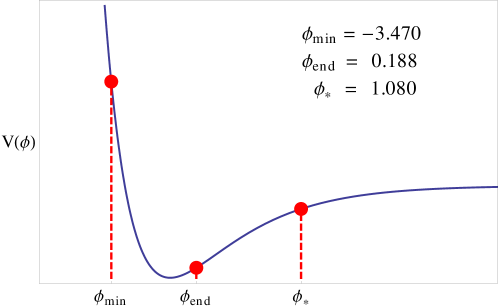
Remark: In order to compute the mass parameter $M$, we have used observational data and assumed the standard power-law power spectrum obtained from standard inflation where perturbations are taken to be in Bunch-Davies state at the onset of inflation. As we will see later in this paper, however, in LQC modes are not in a Bunch-Davies state at the onset of inflation and the power spectrum is not exactly the same as the standard one. There are corrections for small $k$ modes while there is agreement for large $k$. Due to these corrections, our computation of $M$ is internally inconsistent. Strictly speaking, one should use the true LQC power spectrum in order to compute the mass parameter. This requires significant numerical work to perform analysis over the whole parameter space, which has been recently done for the quadratic potential in agullomorris . They find that, while using the LQC power spectrum to compute $M$ is conceptually important, it leads to very small corrections in the power spectra and the main results remain unchanged. We expect a similar conclusion for the Starobinsky potential. Nevertheless, it is an important issue and we leave it for future investigations. In this paper, we bypass this issue by choosing initial conditions for which the reference mode corresponds to large enough $k$ where the Bunch-Davies and LQC power spectra differ very little. Therefore, any correction to $M$, if any, would be too small to impact our results.

III.2 Initial states for quantum perturbations

In de Sitter spacetime one can construct a unique vacuum state for linear, cosmological perturbations that are regular and respect the symmetries of the de Sitter background. These vacuum states are the so-called Bunch-Davies states. In the standard inflationary scenario the spacetime metric can be approximated by a de Sitter metric at the onset of slow-roll. Therefore, it is a reasonable assumption that the observable modes are in the Bunch-Davies state there. In LQC, on the other hand, the modified pre-inflationary dynamics extends all the way to the Planck scale where the background is very different from de Sitter spacetime. Therefore, quantum perturbations cannot be chosen to be in a Bunch-Davies state close to the bounce. As suggested in aan2 ; aan3 ; ana , one can still use the physical principles behind the construction of Bunch-Davies states to obtain vacuum states in LQC. These principles require that the states should be ultraviolet regular and invariant under the symmetries of the underlying spacetime, which in our case is given by the dressed metric $\tilde{g}_{ab}$ (Sec. II.2). This leads us to a 4th order adiabatic state at bounce. It turns out that if the states are chosen to be 4th order adiabatic initially, they remain so throughout the evolution. Another physical input used in the choice of states stems from the test field approximation. That is, the backreaction of the quantum perturbations on the background spacetime in quantum gravity regime is negligible. This is essential for the self-consistency of the dressed metric approach.

Unlike in de Sitter spacetime, however, this procedure does not single out a unique vacuum state. In this paper, we will use four different types of states, which are based on different physical principles:

• Type I: this vacuum state is constructed such that it leads to suppression of power at large scales in the CMB as suggested in ag2 ;

• Type II: this vacuum state minimizes the stress energy tensor of the perturbations to zero at some initial time (called ‘instantaneous vacuum’ in ana );

• Type III: this vacuum state is the approximate WKB solution of the evolution equations at some initial time (called ‘obvious vacuum’ in aan3 ); and

• Type IV: this vacuum state is a combination of the type II vacuum for large $k$ and a Minkowski-like vacuum for small $k$ as suggested in agulloassym .

Note that these initial states are not specified at the bounce, but slightly before the bounce (specifically, at $t=-10\,s_{\rm Pl}$) for technical reasons that arise for infrared modes.

IV Results

Let us now turn to the numerical results. Recall that according to the framework of quantum field theory on quantum spacetime, as long as the perturbations can be treated as test fields, the information about the background geometry that is relevant for the evolution of perturbations can be encoded into a dressed effective geometry. The dressed metric is obtained from the expectation values of only certain moments of the scale factor and field momentum with respect to the background wavefunction $\Psi(a,\phi)$ eq. (9). One does not need all the details of the quantum fluctuations of the wavefunction in order to determine the behavior of the quantum perturbations. Strictly speaking, given a state $\Psi$ in the physical Hilbert space, the dressed (denoted with $tilde$ on top) and the effective scale factor are different from each other. However, as shown via explicit numerical simulations in ag1 , the numerical differences between the dressed metric and the effective metric is very small (less than a percent) for sharply peaked states ($\Delta V/V\ll 1$). In this paper, we consider such sharply peaked states and approximate the dressed geometry with the effective geometry discussed in Sec. II.1.

The remainder of this section is divided into three subsections. In the first, we explore the evolution of the background effective geometry for various classes of initial conditions. We find the subset of initial conditions that leads to the desired slow-roll phase, which is necessary for compatibility with observations. As expected, the occurrence of the quantum bounce is a generic feature of the loop quantum geometry and the desired slow-roll phase happens for almost all of the initial conditions. In the second subsection, we describe why the pre-inflationary dynamics matters for perturbations and how the ultraviolet quantum gravity effects can lead to particle production for infrared modes of perturbations. Finally in the third subsection, we present the numerical evolution of the scalar and tensor perturbations on this effective background geometry, compute their power spectra at the end of inflation, and extract the window of initial conditions relevant for observational consequences of pre-inflationary dynamics of LQC. Evolution of the background geometry in the quantum gravity regime, and that of the quantum perturbations, turns out to be mostly similar to that for the quadratic potential studied in aan3 . However, there is a small subset of initial conditions for which Starobinsky potential leaves different signatures for very long wavelength modes.

Figure 2: Evolution of the scale factor with $\phi_{{}_{\rm B}}=-1.45$ and $\dot{\phi}_{{}_{\rm B}}>0$. The (red) solid curve and the (blue) dashed curve respectively show the evolution of the scale factors in LQC and classical GR. The bounce happens at $t=0$ where the classical trajectory goes to big bang singularity. Following the bounce, there is short phase of super-inflation which ends at $t\sim 0.19\,t_{\rm Pl}$. In the future evolution LQC and classical GR trajectory converge. The inset shows the late time evolution of the LQC scale factor undergoing inflation which ends at $t\sim 6\times 10^{7}\,t_{\rm Pl}$.

Figure 3: The energy density of the matter field (left panel) and the evolution of the scalar field (right panel) for the same initial conditions as in Fig. 2. The energy density in LQC has a maximum at the bounce while in classical GR it diverges. The scalar field evolves from negative values to the positive valued slow-roll side of the potential. The insets show the late time evolution of $\rho$ and $\phi$. During inflation the energy density is of the order of $10^{-12}\,\rho_{\rm Pl}$ and remains almost constant. At the end of inflation there is a drop in $\rho$ while the scalar field oscillates at the minimum of the potential around $\phi=0$.

IV.1 Background evolution

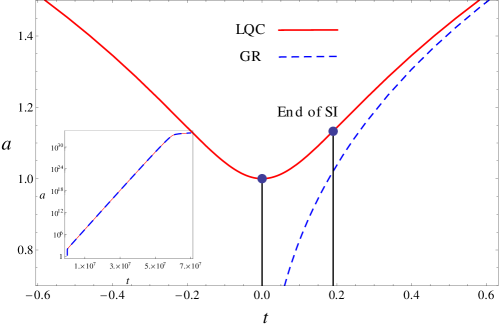
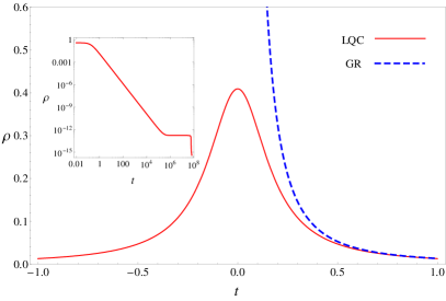
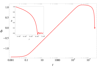
Fig. 2 shows the evolution of the scale factor in LQC (solid curve) and classical GR (dashed curve) for a representative case with $\phi_{{}_{\rm B}}=-1.45~{}m_{\rm Pl}$ and $\dot{\phi}_{{}_{\rm B}}>0$. The corresponding energy density and the scalar fields are shown in Fig. 3. From these plots, it is immediately obvious that in the vicinity of the quantum bounce, which is well inside the Planckian regime, there are significant deviations between classical GR and LQC: First, the scale factor bounces from a non-zero value in LQC while in the classical theory $a\rightarrow 0$. Second, the energy density is finite at the bounce for the LQC evolution, but diverges in classical GR. Following the quantum bounce, there is a brief phase ($\sim 0.2\,t_{\rm Pl}$) of faster than exponential accelerated expansion, called super-inflation. During this phase the Hubble rate quickly grows from zero to its maximum value. At the end of super-inflation, characterized by $H=H_{\rm max}$ (and, consequently, $\dot{H}=0$), the energy density of the scalar field is half of that at the bounce (see eq. (4)). This super-inflationary phase is the most quantum gravity dominated part of the evolution. In further evolution, the Hubble rate, the energy density and hence the spacetime curvature decrease monotonically while the scale factor grows. After approximately a hundred Planck seconds, the spacetime curvature falls well below the Planckian value where LQC and classical GR are in excellent agreement with each other. The desired phase of slow roll inflation begins typically when the energy density becomes of the order of $10^{-12}\,\rho_{\rm Pl}$. Recall that by slow roll, we mean the period between when $k_{*}$ exited the horizon to when the first Hubble slow-roll parameter becomes equal to one. At the onset of this slow-roll phase $\phi$ and $\dot{\phi}$ attain the values in (23). Note that by definition the number of e-folds during this slow-roll phase of inflation is 58 for the Starobinsky potential, but the total number of e-folds during the entire inflationary epoch (when $\ddot{a}>0$) can be much higher.

The right panel of Fig. 3 shows the corresponding evolution of the scalar field with the same initial conditions. The scalar field starts from the left side of the minimum of the potential (see Fig. 1) with a positive $\dot{\phi}_{{}_{\rm B}}$ due to which it rolls down the potential. As the further evolution takes place, the field crosses the minimum and starts climbing up on the slow-roll side and at some point in the evolution crosses $\phi_{*}$ for the first time. But this time the field has a positive velocity and does not have the correct slow-roll parameters. Due to the remaining kinetic energy, the field climbs a little higher up the potential until KE=0, and that is when the field turns around and starts rolling down the potential with $\dot{\phi}<0$. In what follows, the field crosses $\phi_{*}$ once more, this time with $\dot{\phi}<0$ and the slow-roll conditions are met. When $\phi$ becomes 0.19 $m_{\rm Pl}$ the slow-roll phase ends and the field continues to roll down the potential and finally oscillates at the minimum of the potential around $\phi=0$ as shown in the inset of the right plot in Fig. 3. Note that, if the field did not have enough kinetic energy to climb high enough the potential and cross $\phi_{*}$ during the climb, the slow-roll conditions would not have been obtained.

Let us now study the evolution of the background geometry in some more detail for a variety of cases by giving the initial conditions at the bounce. We will divide the set of initial conditions into two classes: (i) positive inflaton velocity ($\dot{\phi}_{{}_{\rm B}}>0$) and (ii) negative inflaton velocity ($\dot{\phi}_{{}_{\rm B}}<0$), and track the evolution of $\phi$, $\dot{\phi}$ and $a$ for different $\phi_{{}_{\rm B}}$. As discussed in Sec. III, the range of $\phi_{{}_{\rm B}}$ is semi-infinite: $\phi_{{}_{\rm B}}\in(\phi_{\rm min},~{}\infty)$ where $\phi_{\rm min}=-3.47~{}m_{\rm Pl}$ corresponds to the extreme potential energy dominated bounce with zero kinetic energy and $\phi_{{}_{\rm B}}\rightarrow\infty$ to the extreme kinetic energy dominated bounce with zero potential energy. As we will see in this section – irrespective of the sign of $\dot{\phi}_{{}_{\rm B}}$ – the potential energy dominated bounces never give rise to the desired phase of slow-roll. This is in contrast to the quadratic potential where the potential energy dominated cases are in fact the ones with large $\phi_{{}_{\rm B}}$ resulting into a huge amount of slow-roll inflation.

IV.1.1 Positive inflaton velocity: $\dot{\phi}_{{}_{\rm B}}>0$

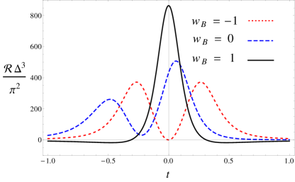
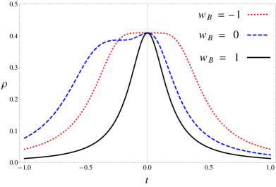
Let us begin by discussing the evolution of the Ricci curvature scalar $\mathcal{R}$ in the quantum gravity regime. The behavior of the Ricci scalar is critical in understanding the evolution of the quantum perturbations, as the Ricci scalar determines the length scale at which the properties of the curved background become important and the quantum perturbation can no longer be treated as fields propagating on a flat background. The expression for the Ricci scalar in terms of the Hubble rate $H$ is:

$$\mathcal{R}=6\left(\dot{H}+2H^{2}\right),$$ (25)

where the dot represents the derivative with respect to the proper time. Now substituting the expressions of $H$ and its derivative in terms of the energy density of the matter field, we have:

$$\mathcal{R}=-24\pi G\,\rho(1+w)\left(1-2\frac{\rho}{\rho_{{}_{\rm max}}}\right)+24\pi G\,\rho\left(1-\frac{\rho}{\rho_{{}_{\rm max}}}\right),$$ (26)

where, as before, $w$ is the polytropic index appearing in the equation of state of the matter field. It is clear from the above equation that specifying the energy density of the matter field and its equation of state completely determines the Ricci curvature. At the bounce, where $\rho=\rho_{{}_{\rm max}}$, we have:

$$\mathcal{R}_{\rm B}=24\pi G\,\rho_{{}_{\rm max}}\,(1+w_{\rm B})=\frac{432~{}\pi^{2}}{\Delta^{3}~{}l_{\rm Pl}^{2}}(1+w_{\rm B}).$$ (27)

In this way, while the maximum of the energy density at the bounce is fixed at $\rho_{{}_{\rm max}}$, the value of the Ricci scalar at the bounce depends on the type of matter field under consideration. For example, for dust $\mathcal{R}_{\rm B}^{\rm(dust)}=\frac{432~{}\pi^{2}}{\Delta^{3}~{}l_{\rm Pl}^{2}}$, for radiation $\mathcal{R}_{\rm B}^{\rm(rad)}=\frac{576~{}\pi^{2}}{\Delta^{3}~{}l_{\rm Pl}^{2}}$ and for a stiff fluid –which is equivalent to a massless scalar field– $\mathcal{R}_{\rm B}^{\rm(stiff)}=\frac{864~{}\pi^{2}}{\Delta^{3}~{}l_{\rm Pl}^{2}}$.

Figure 4: Plots of the Ricci scalar and energy density near the bounce (left and right panel, respectively). For the extreme potential energy dominated case ($w_{\rm B}=-1$), the Ricci scalar vanishes at the bounce, whereas for the extreme kinetic energy dominated case ($w_{\rm B}=1$), the Ricci scalar is maximum at the bounce. The energy density is maximum at the bounce for all cases. For the intermediate case when the potential and kinetic energy are exactly equal at the bounce ($w_{\rm B}=0$), the Ricci scalar $\mathcal{R}_{\rm B}$ is half of the maximum value attained for $w_{\rm B}=1$. For all conditions $w_{\rm B}<1$, the Ricci scalar behaves non-monotonically in the future evolution. Moreover, the bounce is time-reversal symmetric for $w_{\rm B}=1$ and $-1$, while asymmetric for all other initial conditions. It is also apparent that the energy density falls more quickly for kinetic energy dominated cases than potential energy dominated ones. Hence, the quantum gravity regime last longer for potential energy dominated bounces.

Table 1: Dynamical evolution for various $\phi_{{}_{\rm B}}$ with $\dot{\phi}_{{}_{\rm B}}>0$. The value of $\phi$, $w$, $t$, $H$, $\epsilon$ and the total number of e-folds since the bounce $N$ is shown for various events. In particular, the events considered are the bounce, end of super-inflation (SI), moment when the kinetic energy equals the potential energy (KE=PE), onset of the desired slow-roll phase (onset) and end of slow roll inflation (end). The zeros in the table are in fact $\mathcal{O}(\epsilon_{machine})$, but from analytic considerations we know these values are identically zero. The last three rows all satisfy $w_{\rm B}-1<10^{-7}$.

Event	$\phi$	$w$	t	$H$	$\epsilon$	N
Bounce	-3.47	-1	0	0	$\infty$	0
End SI	-3.25	0.32	0.46	0.93	0	0.20
KE=PE	-0.55	0	$4.7\times 10^{4}$	$1.5\times 10^{-5}$	1.5	8.12
Onset	NA	NA	NA	NA	NA	NA
End	NA	NA	NA	NA	NA	NA
Bounce	-3.39	0	0	0	$\infty$	0
End SI	-3.21	0.52	0.26	0.93	0	0.16
KE=PE	-0.54	0	$4.7\times 10^{4}$	$1.5\times 10^{-5}$	1.5	7.87
Onset	NA	NA	NA	NA	NA	NA
End	NA	NA	NA	NA	NA	NA
Bounce	-1.49	1.0	0	0	$\infty$	0
End SI	-1.35	1.0	0.18	0.93	0	0.12
KE=PE	0.91	0	$2.4\times 10^{5}$	$1.7\times 10^{-6}$	1.5	4.74
Onset	NA	NA	NA	NA	NA	NA
End	NA	NA	NA	NA	NA	NA
Bounce	-1.45	1.0	0	0	$\infty$	0
End SI	-1.31	1.0	0.18	0.93	0	0.12
KE=PE	0.95	0	$2.4\times 10^{5}$	$1.7\times 10^{-6}$	1.5	4.74
Onset	1.08	-1.0	$2.7\times 10^{6}$	$1.2\times 10^{-6}$	$1.9\times 10^{-4}$	7.90
End	0.19	-0.67	$5.2\times 10^{7}$	$7.4\times 10^{-7}$	0.50	67.14
Bounce	-1.41	1.0	0	0	$\infty$	0
End SI	-1.27	1.0	0.18	0.93	0	0.12
KE=PE	0.99	0	$2.4\times 10^{5}$	$1.7\times 10^{-6}$	1.5	4.74
Onset	1.08	-1.0	$1.2\times 10^{7}$	$1.2\times 10^{-6}$	$1.9\times 10^{-4}$	19.35
End	0.19	-0.67	$6.1\times 10^{7}$	$7.4\times 10^{-7}$	0.50	78.59

As a result, this is where one of the main distinctions between the potential and kinetic energy dominated bounces appears. For kinetic energy dominated bounces, $w_{\rm B}\approx 1$ and consequently $\mathcal{R}_{\rm B}^{\rm(kin)}\approx\frac{864~{}\pi^{2}}{\Delta^{3}~{}l_{\rm Pl}^{2}}$. On the other hand, for potential energy dominated bounces, when the kinetic energy is close to zero, $w_{\rm B}\approx-1$ and $\mathcal{R}_{\rm B}^{\rm(pot)}\approx 0$. That is, the Ricci curvature at the bounce is maximized for kinetic energy dominated bounces, but vanishes for potential energy dominated bounces. Thus, for positive potentials, while the energy density always saturates its maximum at the bounce, the Ricci scalar does not. As a result, the evolution of the Ricci scalar to the future of the bounce is not necessarily monotonic, unlike the evolution of the energy density. In Fig. 4, we show the evolution of the Ricci scalar for kinetic and potential energy dominated as well as for an intermediate case with $w_{\rm B}=0$ at the bounce. It is clear that for $w_{\rm B}=-1$ (extreme potential energy domination) the Ricci curvature vanishes at the bounce, then attains a local maximum and falls in the future evolution. For $w_{\rm B}=1$ (extreme kinetic energy domination) the Ricci curvature is maximum at the bounce and fall monotonically in the future evolution. It is also interesting to see that the maximum value that the Ricci scalar attains in its future evolution for $w_{\rm B}=-1$ is less than that for $w_{\rm B}=1$. Hence, the curvature scalars for different initial conditions are drastically different close to the bounce in the quantum gravity regime. This is conceptually important as this implies that the modes of quantum perturbations will be excited in qualitatively different ways depending on whether the bounce is potential or kinetic energy dominated. Furthermore, the energy density falls of slower for potential energy dominated cases and therefore the quantum gravity regime lasts longer. However, it turns out that this interesting conceptual difference is not relevant for observations since the potential energy dominated bounces do not lead to enough e-folds during slow-roll and thus are not compatible with observations.

For our numerical simulations, we used the Runge-Kutta numerical integration scheme in Mathematica 10 and performed over a hundred simulations. Table 1 shows some of the representative simulations for various $\phi_{{}_{\rm B}}$ when the initial velocity of the inflaton is positive. We are interested in the following events during the evolution: (i) bounce, (ii) end of super-inflation, (iii) equivalence of kinetic and potential energy (specifically, $w=0$), (iii) onset of the desired slow-roll phase and (iv) end of inflation. For each initial condition, we compute the following values at these events: $\phi$, $w$, $t$, $H$, $\epsilon$ and the total number of e-folds since the bounce $N$. The first two initial conditions in the table correspond to an extreme potential energy dominated case ($w_{\rm B}=-1$) and an equal distribution between kinetic and potential energy ($w_{\rm B}=0$). The remaining three entries correspond to initial conditions for which the kinetic energy dominates over the potential energy by a factor of $10^{7}$ or more. Duration of super-inflation is largest for the first row, slightly smaller for the second row. For the rest of the entries in the table the evolution remains almost the same till KE=PE. This happens because in the first two rows, potential does affect the evolution near the bounce, while for the rest of the cases shown in the table the field behaves almost like a massless scalar and potential becomes relevant after KE=PE. It is apparent from the table that the total number of e-folds for $\phi_{{}_{\rm B}}\in(\phi_{\rm min},-1.45)$, which are potential energy dominated initial conditions, is less than 60. Hence, the desired slow-roll marked by $\epsilon_{*}=0.00019$ and $\delta_{*}=-0.017$ is not obtained. On the other hand, for $\phi_{{}_{\rm B}}\geq-1.45$ (which is kinetic energy dominated) the desired phase of slow-roll is necessarily contained in the evolution. Clearly, the potential energy dominated bounces are not compatible with observations. The reason for this is that these potential energy dominated bounces do not have enough initial kinetic energy to climb up the potential on the other side and reach $\phi_{*}$.

Table 2: Dynamical evolution for various $\phi_{{}_{\rm B}}$ with $\dot{\phi}_{{}_{\rm B}}<0$. The table is structured the same way as Table 1: Shown are the values of $\phi$, $w$, $t$, $H$, $\epsilon$ and the total number of e-folds since the bounce $N$ for several events. In particular, the events considered are the bounce, end of super-inflation (SI), when the kinetic energy equals the potential energy (KE=PE), at the onset of the desired slow-roll phase (onset) and at the end of slow roll inflation (end). The first row corresponds to an initial condition with equal amounts of potential and kinetic energy, the second row has $w_{\rm B}=1$ and the remaining four rows satisfy $w_{\rm B}-1<10^{-12}$.

Event	$\phi$	$w$	t	$H$	$\epsilon$	N
Bounce	-3.39	0	0	0	$\infty$	0
End SI	-3.46	-1.0	0.22	0.93	0	0.07
KE=PE	-0.55	0	$4.7\times 10^{5}$	$1.5\times 10^{-5}$	1.5	8.46
Onset	NA	NA	NA	NA	NA	NA
End	NA	NA	NA	NA	NA	NA
Bounce	0	1	0	0	$\infty$	0
End SI	-0.14	1.0	0.18	0.93	0	0.12
KE=PE	-1.43	0	$6.2\times 10^{2}$	$6.2\times 10^{-4}$	1.5	2.73
Onset	NA	NA	NA	NA	NA	NA
End	NA	NA	NA	NA	NA	NA
Bounce	3.00	1.0	0	0	$\infty$	0
End SI	2.86	1.0	0.18	0.93	0	0.12
KE=PE	0.59	0	$2.6\times 10^{5}$	$1.6\times 10^{-6}$	1.5	4.77
Onset	NA	NA	NA	NA	NA	NA
End	NA	NA	NA	NA	NA	NA
Bounce	3.63	1.0	0	0	$\infty$	0
End SI	3.49	1.0	0.18	0.93	0	0.11
KE=PE	1.23	0	$2.4\times 10^{5}$	$1.7\times 10^{-6}$	1.5	4.74
Onset	1.08	-1.0	$2.7\times 10^{6}$	$1.2\times 10^{-6}$	$2.0\times 10^{-4}$	7.84
End	0.19	-0.69	$5.2\times 10^{7}$	$7.4\times 10^{-7}$	0.50	67.07
Bounce	3.67	1.0	0	0	$\infty$	0
End SI	3.52	1.0	0.18	0.93	0	0.12
KE=PE	1.27	0	$2.4\times 10^{5}$	$1.7\times 10^{-6}$	1.5	4.74
Onset	1.08	-1.0	$1.2\times 10^{7}$	$1.2\times 10^{-6}$	$1.9\times 10^{-4}$	19.37
End	0.19	-0.69	$6.1\times 10^{7}$	$7.4\times 10^{-7}$	0.50	78.61
Bounce	4.00	1.0	0	0	$\infty$	0
End SI	3.86	1.0	0.18	0.93	0	0.12
KE=PE	1.60	0	$2.3\times 10^{5}$	$1.8\times 10^{-6}$	1.5	4.74
Onset	1.08	-1.0	$1.9\times 10^{8}$	$1.2\times 10^{-6}$	$1.9\times 10^{-4}$	239
End	0.19	-0.69	$2.4\times 10^{8}$	$7.4\times 10^{-7}$	0.50	298

Figure 5: These plots show the Ricci scalar (left panel) and energy density (right panel) near the bounce for $\dot{\phi}_{{}_{\rm B}}<0$. Similar to Fig. 4, the Ricci scalar at the bounce is zero for the extreme potential energy dominated case ($w_{\rm B}=-1$) and maximum for the extreme kinetic energy dominated case ($w_{\rm B}=1$). Also, the energy density is maximum at the bounce for all cases. For the intermediate case when the potential and kinetic energy are equal at the bounce ($w_{\rm B}=0$), the maximum of the Ricci scalar does not occur at the bounce. For all initial conditions with $w_{\rm B}<1$, the Ricci scalar behaves non-monotonically in the future evolution. Moreover, the bounce is time-reversal symmetric only for $w_{\rm B}=1$ and $w_{\rm B}=-1$. It is noteworthy that for $-1<w_{\rm B}<1$, the behavior of $\mathcal{R}$ and $\rho$ is the mirror image of those in Fig. 4.

IV.1.2 Negative inflaton velocity: $\dot{\phi}_{{}_{\rm B}}<0$

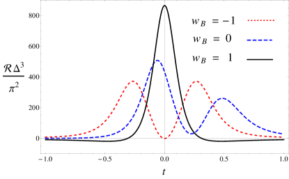
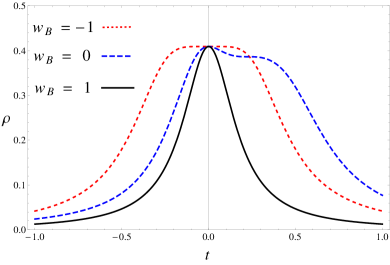
Let us now consider initial data with negative initial inflaton velocity. Fig. 5 shows the evolution of the Ricci scalar and the energy density for three different equations of state at the bounce: $w_{\rm B}=1,0,-1$. Similar to the positive $\dot{\phi}_{{}_{\rm B}}$ case, $\mathcal{R}$ at the bounce is zero for $w_{\rm B}=-1$, maximum for $w_{\rm B}=1$ and half the maximum value for $w_{\rm B}=0$. Also, the evolution of $\mathcal{R}$ is time-reversal symmetric for $w_{\rm B}=1$ and $w_{\rm B}=-1$, but asymmetry for all other initial conditions. Interestingly, this time reversal asymmetry is the mirror image of the asymmetry for positive $\dot{\phi}_{{}_{\rm B}}$ (Fig. 4).

Similar to Table 1, Table 2 shows some of the representative simulations for various initial conditions. The first row corresponds to $w_{\rm B}=0$ and all other rows have $w_{\rm B}\approx 1$. It turns out that, similar to the positive $\dot{\phi}_{{}_{\rm B}}$ case, the potential energy dominated initial conditions do not lead to the desired slow-roll phase. The second row corresponds to the extreme kinetic energy dominated case with exactly zero potential energy at the bounce. Unlike in the the positive $\dot{\phi}_{{}_{\rm B}}$ case this initial condition does not contain the desired slow-roll phase in its future evolution. The reason for this asymmetry between positive and negative $\dot{\phi}_{{}_{\rm B}}$ is that for negative $\dot{\phi}_{{}_{\rm B}}$ the inflaton initially evolves to the left of the potential (see Fig. 1) and in fact reaches $\phi_{*}$ very quickly, however, when it does so, its kinetic energy is too large and therefore the slow-roll parameters are too large and the desired phase of slow-roll does not start. This does not immediately imply that slow-roll will not occur at all, because when the field rolls back from the left side of the potential it might be possible that it climbs up the potential and reach $\phi_{*}$ again, now with significantly less kinetic energy. Simulations show that this scenario did not happen, because the field loses a lot of kinetic energy due to both Hubble friction and the steepness of the potential, consequently, it does not have enough kinetic energy to climb up the potential on the slow-roll side and reach $\phi_{*}$. Thus, this means that for the desired slow-roll phase to happen with $\dot{\phi}_{{}_{\rm B}}<0$, the inflaton field has to start high enough on the slow-roll side. As the table shows, $\phi_{{}_{\rm B}}\geq 3.63$ for the desired slow-roll phase to occur in the future evolution.

Figure 6: $\phi-\dot{\phi}$ phase portrait of evolution trajectories for Starobinsky potential in LQC. All trajectories (shown by curves with arrowheads) start at the bounce which is given by constant density surface $\rho=\rho_{{}_{\rm max}}$ (shown by the thick black boundary curve without arrowheads). The bounce surface extends from $\phi=-3.47~{}m_{\rm Pl}$ all the way to $\infty$, but here we have only shown a part of it. The dashed (blue) curves do not lead to the desired slow-roll, while the solid (red) ones do. Since the diagram extends all the way to $\phi=\infty$, the fraction of dashed (blue) curves is extremely small compared to the solid ones. Therefore, it can be concluded that the occurrence of slow-roll is almost inevitable.

IV.1.3 Phase portrait and the desired slow-roll

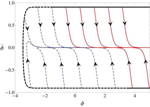
Looking at Table 1 and Table 2, we conclude that observationally compatible initial conditions are: $\phi_{{}_{\rm B}}\geq-1.45\,m_{\rm Pl}$ for positive $\dot{\phi}_{{}_{\rm B}}$ and $\phi_{{}_{\rm B}}\geq 3.63\,m_{\rm Pl}$ for negative $\dot{\phi}_{{}_{\rm B}}$. Thus, in the entire parameter space of the initial conditions it is only the kinetic energy dominated initial conditions which lead to the desired slow-roll phase in their future evolution; there is a subset, rather small however, of the kinetic energy dominated initial conditions which do not give desired slow-roll. Fig. 6 shows some of the representative trajectories of evolution in a $(\phi,\,\dot{\phi})$ phase diagram starting from the initial data surface (thick black curve without arrowheads). As discussed in Sec. III the initial data surface is non-compact: while $|\dot{\phi}_{{}_{\rm B}}|<0.91\,m_{\rm Pl}^{2}$, $\phi_{{}_{\rm B}}$ is not restricted to a finite interval, that is, $\phi_{{}_{\rm B}}\in\left[-3.47\,m_{\rm Pl},\infty\right)$. The blue, dashed trajectories are the ones which do not lead to the desired slow-roll in their future evolution, while the red, solid trajectories are the ones which do. In the same way, the dashed part of the initial data surface corresponds to the subset of initial data that is not compatible with observations while the solid part (which continues to $\phi\rightarrow\infty$) is compatible. Clearly, the part that does not lead to the desired phase of slow-roll is negligible compared to the entire initial data surface. In this sense, a significantly high fraction of initial data lead to the desired slow-roll and inflation is almost inevitable.

IV.1.4 Comparison with quadratic potential

There are some interesting differences and similarities between inflation with a quadratic potential and with the Starobinsky potential. In particular, while potential energy dominated bounces lead to an enormous amount of inflation for the quadratic potential, they do not lead to enough inflation to be compatible with observations for the Starobinsky potential. As a result, in Starobinsky inflation, only (a large subset of) kinetic energy dominated bounces are compatible with observations, whereas for inflation with a quadratic potential both kinetic and potential energy dominated bounces are compatible with observations.

For kinetic energy dominated bounces, the details of the potential do not matter in the early evolution, in other words, the evolution is driven by the kinetic energy. Consequently, the evolution of a kinetic energy dominated bounce in Starobinsky inflation will be similar to the evolution of a kinetic energy dominated bounce with a quadratic potential. Since the quantum gravity effects stem from exactly this period, one can expect that the quantum geometry corrections to the standard inflationary paradigm will be similar for Starobinsky inflation and kinetic energy dominated bounces in a quadratic potential. This expectation will indeed be borne out in the next subsections. There are, however, some surprises for extremely long wavelength modes that are larger than the observable universe.

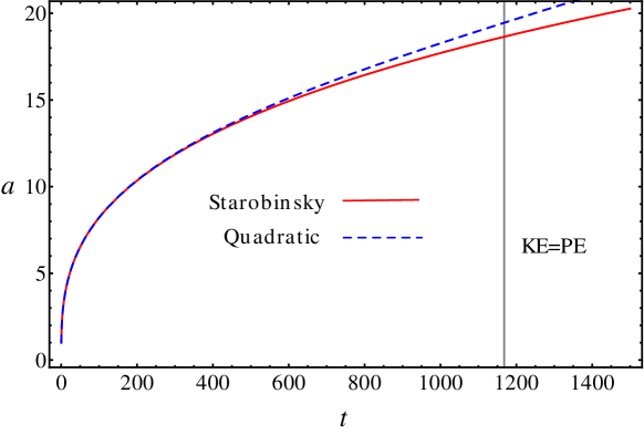
To see explicitly that the evolution is indeed similar, Fig. 7 shows a plot of the scale factor, which captures all the geometric information, evolved for inflation with a scalar field in the quadratic potential and Starobinsky potential. In order for this comparison to be meaningful, we took $w_{\rm B}$ to be the same for both models, in particular, $w_{\rm B}=0.9999999618$. This does not completely fix $\phi_{{}_{\rm B}}$ and $\dot{\phi}_{{}_{\rm B}}$: there is some freedom in overall signs left. We took the signs to be the same for both models, specifically, $\phi_{{}_{\rm B}}=-92.14\,m_{\rm Pl}$ and $\dot{\phi}_{{}_{\rm B}}>0$ for the quadratic potential and $\phi_{{}_{\rm B}}=-1.45\,m_{\rm Pl}$ and $\dot{\phi}_{{}_{\rm B}}>0$ for the Starobinsky potential. Note that around $t\approx 600\,s_{\rm Pl}$ the two geometries start to deviate slowly. This is when $w\approx 0.6$ for the quadratic potential (for the Starobinsky potential it is still very close to its value at the bounce). By the time $t=1168\,s_{\rm Pl}$, the scalar field in the quadratic potential has lost half of its initial energy to potential energy and the two geometries start to deviate more and more. Thus, indeed the details of the potential are irrelevant close to the bounce for kinetic energy dominated bounces as far as the background geometry is concerned. Note that this is true for all kinetic energy dominated bounces and does not require the initial conditions to be ‘close’ to the bottom of the potential, where the Starobinsky potential can be considered to be well approximated by the quadratic potential. Clearly, after the kinetic energy equals the potential energy, the features of the potential become more important. This occurs, however, well into the regime where classical GR is in excellent agreement with the effective equations of LQC and is thus irrelevant for the quantum geometric corrections (but is very important for the predictions within the standard inflationary paradigm!).

Figure 7: Plot of the evolution of the scale factor for two different cases: quadratic potential (blue, dashed) and the Starobinsky potential (red, solid). The gray vertical line at $t=1168\,s_{\rm Pl}$ indicates when the kinetic energy becomes equal to the potential energy for the quadratic potential (for the Starobinsky potential this occurs much later, see Table 2). Both cases are kinetic energy dominated bounces with the same value of $w$ at the bounce, that is, $w_{\rm B}=0.9999999618$. This determines $\phi_{{}_{\rm B}}$ and $\dot{\phi}_{{}_{\rm B}}$ up to signs. We choose the same signs for the quadratic and Starobinsky potential for easier comparison. In particular, $\phi_{{}_{\rm B}}=-92.14\,m_{\rm Pl}$ and $\dot{\phi}_{{}_{\rm B}}>0$ for the $\phi^{2}$ potential and $\phi_{{}_{\rm B}}=-1.45\,m_{\rm Pl}$ and $\dot{\phi}_{{}_{\rm B}}>0$ for the Starobinsky potential.

IV.2 Phenomenological considerations

Figure 8: Evolution of two observable modes and the physical curvature length scale: in the classical theory close to singularity (shown in the left panel) and in LQC close to the quantum bounce (shown in the right panel). It is clear that the physical wavelengths of both modes remain smaller than the curvature length scale in the classical theory all the way to the big bang. Whereas one of the modes in LQC becomes larger than the non-zero curvature length scale at the bounce. This mode gets excited in the future evolution.

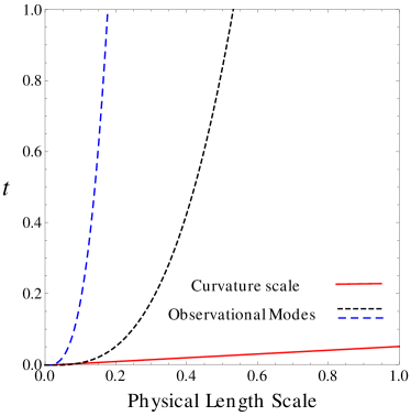
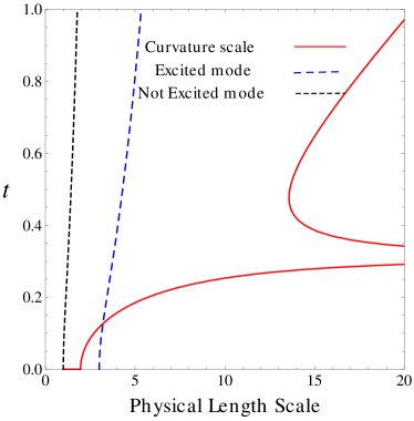
Before we move to the discussion of the power spectra of quantum perturbations, some phenomenological considerations are in order. So far, in this paper, we have seen that the inflationary scenario with a Starobinsky potential (14) fits well with the non-singular bouncing picture of LQC: The pre-inflationary dynamics of the background spacetime is significantly modified due to the quantum geometric effects for energy scales in the regime $10^{-3}\rho_{{}_{\rm max}}<\rho<\rho_{{}_{\rm max}}$. As a result, quantum perturbations in LQC experience a very different history before the onset of inflation compared to the quantum perturbations in the standard inflationary scenario based on GR. There is a finite non-zero length scale associated to the maximum value of the Ricci curvature scalar, $k_{\rm LQC}:=(\mathcal{R}_{\rm B}/6)^{1/2}$, due to which modes of different wavelengths interact with the curvature in a qualitatively different way. Ultraviolet modes ($k\gg k_{\rm LQC}$) are too energetic to be affected by the curvature and evolve as if they are in a flat spacetime, whereas mode with small wavenumber ($k\sim k_{\rm LQC}$) do get excited by the curvature. This can be understood via Fig. 8, which shows the evolution of two observable modes in GR (in the left panel) and LQC (in the right panel). In GR, all observable modes remain smaller than the curvature length scale all the way to the big bang. In LQC, on the other hand, there are some modes which are larger than the curvature length scale near the bounce. It is these infrared modes that will be excited in their future evolution and deviate from the usual Bunch-Davies state at the onset of inflation.

CMB experiments, such as Planck and WMAP, report the value of the amplitude and the spectral index of the power spectrum at a reference mode which is given by a comoving wavenumber $k_{*}$ whose physical wavenumber ($k_{*}/a(t_{*})$) at the time of the horizon crossing is equal to the Hubble parameter at that time, i.e. $k_{*}/a(t_{*})=H_{*}$. Since $k_{*}$ is the comoving wavenumber, its numerical value depends on the numerical value of the scale factor which is different for different conventions. For example, in standard cosmology and also in the phenomenology of CMB experiments the scale factor is chosen to be unity today, whereas in our numerical simulations we have chosen the scale factor to be unity at the bounce. Therefore the numerical value of the comoving wavenumber of the reference mode in LQC, $k_{*}^{\rm LQC}$, will be different from the comoving wavenumber $k_{*}$ at which $A_{\rm s}$ and $n_{\rm s}$ are reported. However, the physical wavenumber corresponding to both $k_{*}^{\rm LQC}$ and $k_{*}$ are still the same, i.e. $k_{*}^{\rm LQC}/a_{\rm LQC}(t_{*})=k_{*}/a_{\rm BD}(t_{*})$. Thus in order to make contact with the observational data we need to find the numerical value of $k_{*}^{\rm LQC}$ that has the same physical wavelength as the reference mode $k_{*}$ at the time of horizon crossing. We adopt the following strategy. We compare the LQC power spectrum at the end of inflation with those predicted by observation and then numerically search for $k$ at which the LQC power spectrum has the same amplitude and Hubble parameter as reported by observations. This $k$ is $k_{*}^{\rm LQC}$. Naturally, the value of $k_{*}^{\rm LQC}$ depends on the amount of e-folds between the onset of slow-roll and the bounce, which can be related to the initial conditions at the bounce: $\phi_{{}_{\rm B}}$ and the sign of $\dot{\phi}_{{}_{\rm B}}$. This relation is shown in Fig. 9.

Figure 9: The reference mode $k^{*}$ shown as a function of $\phi_{{}_{\rm B}}$ which controls the number of e-folds. It is apparent that $k^{*}$ increases with increasing $\phi_{{}_{\rm B}}$.

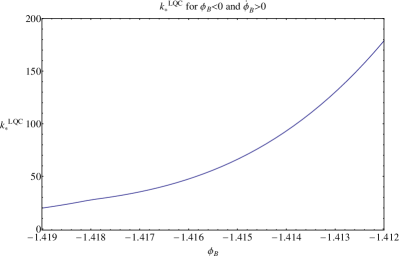
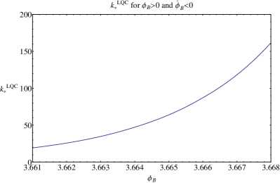
As inflation happens, the infrared modes get stretched to super Hubble size and may no longer fall into the observable window. Therefore not all modes of the perturbations are observable, rather, there is a finite range: $(k_{\rm min},k_{\rm max})\approx(k_{*}^{\rm LQC}/8.58,\,200k_{*}^{\rm LQC})$, where $(k_{\rm min}$ and $k_{\rm max}$ are the co-moving wavenumbers of the longest wavelength entering the Hubble horizon today and the shortest observable modes in the CMB, respectively. If $\phi_{{}_{\rm B}}$ is changed, the value of $k_{*}^{\rm LQC}$ changes as shown in Fig. 9, which will shift the observational window in which LQC effects are observable. On the one hand, if $k_{*}^{\rm LQC}$ is too large then LQC corrections may not be observable at all. On the other hand, if $k_{*}^{\rm LQC}$ is too small then the deviations between the standard inflationary power spectrum and LQC power spectrum may be too large to agree with current observations. Additionally, if $k_{*}^{\rm LQC}$ is too small, numerical investigations have shown that the test field approximation may fail. By demanding that the LQC power spectrum agrees with the standard power spectrum for $\ell\gtrsim 30$ and the backreaction of the perturbations during quantum gravity regime is small, we can further restrict the set of initial conditions that are both observationally interesting and self-consistent with the framework of quantum field theory on quantum spacetime. For a type-I state whose power spectrum is shown in Fig. 10, above requirements lead to the following observationally relevant initial conditions: $-1.419~{}m_{\rm Pl}<\phi_{{}_{\rm B}}<-1.412~{}m_{\rm Pl}$ for positive $\dot{\phi}_{{}_{\rm B}}$ and $3.661~{}m_{\rm Pl}<\phi_{{}_{\rm B}}<3.668~{}m_{\rm Pl}$ for negative $\dot{\phi}_{{}_{\rm B}}$ at the bounce. Note that these initial conditions might vary for different states that have different power spectra.

IV.3 Perturbations

As discussed earlier in this section, depending on the initial value of the inflaton field, the bounce and its subsequent quantum gravity regime can be potential or kinetic energy dominated. For the kinetic energy dominated bounces (with $w_{\rm B}\approx 1$), the background evolution in the quantum gravity regime is practically the same for all potentials, because the scalar field behaves like a massless scalar field. For these initial conditions, the quantum gravity corrections to the inflationary power spectrum for the Starobinsky potential turn out to be qualitatively very similar to that for the quadratic potential. For potential energy dominated bounces, on the other hand, the quantum gravity regime is dictated by the shape of the potential and hence one would expect potential specific features in the inflationary power spectrum. However, as we found in the first part of this section, potential energy dominated initial conditions are not compatible with observations for Starobinsky inflation as they do not lead to the desired slow-roll phase. Hence, given initial conditions for a quadratic potential and Starobinsky potential that lead to the same number of e-folds from the bounce till the end of inflation with $N\gtrsim 60$, the LQC corrections to the observable inflationary power spectra in the two cases are practically indistinguishable. In the following, we will discuss the scalar and tensor power spectra. The initial conditions for perturbations are given slightly before the bounce and then evolved till the end of inflation using eq. (11) and (13).

Figure 10: Scalar power spectrum (left panel) for $\phi_{{}_{\rm B}}=-1.419\,m_{\rm Pl}$ for Starobinsky potential using the type I initial state. The red, solid curve shows the binned LQC spectrum, the black, dashed curve shows the Bunch-Davies power spectrum without LQC modifications and the blue scattered points show the un-binned LQC power spectrum. It is apparent that for large $k$ the LQC power spectrum agrees extremely well with the standard inflationary power spectrum. This behavior is similar to that of a quadratic potential as shown in aan3 .

IV.3.1 Scalar modes

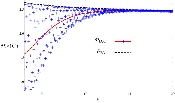
Fig. 10 shows the scalar power spectrum for a representative case with $\phi_{{}_{\rm B}}=-1.45\,m_{\rm Pl}$ and $\dot{\phi}_{\rm B}>0$. This corresponds to a total of $\sim 67$ e-folds from the bounce till the end of inflation. Similar to the quadratic potential (aan3 ), the true LQC power spectrum is oscillatory as shown by the blue “$+$” points in the figure. This oscillatory behavior of the power spectrum can be understood by first writing the mode function of the scalar perturbations as Bogoliubov transformation on the usual Bunch-Davies states:

$$q_{\rm LQC}(k)=\alpha(k)~{}q_{\rm BD}(k)+\beta^{*}(k)~{}q^{*}_{\rm BD}(k).$$ (28)

The LQC power spectrum then can be written as:

$$\mathcal{P}_{\rm LQC}^{(s)}(k)=\mathcal{P}_{\rm BD}^{(s)}(k)|\alpha(k)+\beta^{*}(k)|^{2}=\mathcal{P}_{\rm BD}^{(s)}(k)\left(|\alpha(k)|^{2}+|\beta(k)|^{2}+2|\alpha(k)||\beta(k)|\cos(\theta(k))\right),$$ (29)

where $\theta$ is the relative phase between $\alpha(k)$ and $\beta(k)$ and the superscript ‘$(s)$’ denotes scalar modes. It is the cosine term in the above expression that is responsible for the oscillatory behavior of the power spectrum. This term vanishes when averaged over a window of $k$, and only the $|\alpha(k)|^{2}+|\beta(k)|^{2}$ part remains. It turns out that these oscillations are too rapid to be seen in the CMB as they will be averaged out by the spherical Bessel functions while computing $\mathcal{C}_{\ell}$ at the surface of last scattering. Therefore, what matters for observations is the average value of the power spectrum: $|\alpha(k)|^{2}+|\beta(k)|^{2}$, which can also be obtained by binning the oscillatory power spectrum. Therefore, as far as observations are concerned the LQC corrections to the standard power spectrum is simply a factor of $|\alpha(k)|^{2}+|\beta(k)|^{2}=1+2|\beta(k)|^{2}$ (shown by the red, solid curve in Fig. 10), where $|\beta(k)|^{2}$ is the number density of the particles produced by the pre-inflationary dynamics of LQC with respect to the standard Bunch-Davies vacuum.

The figure clearly shows that only the small $k$ modes deviate from the standard Bunch-Davies power spectrum, while for large $k$ there is remarkable agreement with the standard Bunch-Davies power spectrum. As discussed before, this behavior stems from the fact that modes with $k$ smaller than the characteristic curvature scale ($k_{\rm LQC}=(\mathcal{R}_{\rm B}/6)^{1/2}$) are excited in the quantum gravity regime (Sec. III) and the particle density for those modes is non-zero ($|\beta(k)|>0$). For larger wavenumbers, on the other hand, $|\beta(k)|$ rapidly decays to zero because high $k$ modes are too energetic to be affected by the curvature and as a result do not get excited.

It is apparent from the discussion above that the qualitative features of the LQC corrections to the observable power spectrum for the Starobinsky potential are the same as those for the quadratic potential, and hence robust under the choice of potential. This is surprising given that the dynamics of the inflationary phase is drastically different for both potentials.

Figure 11: Comparison of tensor to scalar ratios in LQC and standard inflation for Starobinsky (with $\phi_{{}_{\rm B}}=-1.419\,m_{\rm Pl}$ and $\dot{\phi}_{{}_{\rm B}}>0$) and quadratic potential (with $\phi_{{}_{\rm B}}=1.16~{}m_{\rm Pl}$). For the quadratic potential $r_{\rm LQC}$ remains extremely close to $r_{\rm BD}$ for all $k$ shown in the diagram while there are departures for the Starobinsky potential. These wavenumbers correspond to modes whose wavelengths are larger than the Hubble horizon. While this effect does not fall into the observable window, it can have non-trivial implications for tensor fossils and non-Gaussian modulation of the power spectrum.

IV.3.2 Tensor modes

Before moving to the discussion of tensor modes for the Starobinsky potenial let us recall the results for the tensor spectrum with a quadratic potential obtained in aan3 . As apparent from eq. (11) and (13), the scalar mode evolution equation involves an effective scalar potential $\tilde{\mathcal{U}}$ which is absent for tensor modes. Therefore, in principle, the particle density for scalar and tensor modes should be different from each other for $k^{2}\approx\tilde{\mathcal{U}}$. However, as shown in aan3 , the magnitude of $\tilde{\mathcal{U}}$ for the quadratic potential is of the order of $10^{-10}~{}k_{\rm min}^{2}$ (where, as before, $k_{\rm min}$ is the smallest value of $k$ that still falls in the observational range of $k$s); therefore the particle density for both the tensor and scalar modes is practically the same. Hence, a significant difference between the tensor and scalar perturbations would be apparent only for $k\sim 10^{-5}k_{\rm min}$ and since the wavenumber of the observable modes are much larger, this difference is not relevant for observations for the quadratic potentials. An immediate consequence of this for the quadratic potential is that the tensor to scalar ratio in LQC is the same as that in standard inflation, that is, $r_{\rm LQC}=r_{\rm BD}$ for all $k\gtrsim 10^{-5}k_{\rm min}$.

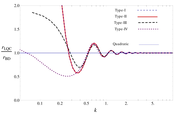
While this is also true for most of the initial conditions for Starobinsky inflation, there does exist a small subset of the initial data surface ($-1.45~{}m_{\rm Pl}\lesssim\phi_{{}_{\rm B}}\lesssim-1.38~{}m_{\rm Pl}$) for which $\tilde{\mathcal{U}}$ is of the order of $10^{-5}k_{\rm min}^{2}$. That is, for $k^{2}\gg k^{2}_{\rm min}10^{-5}$ ($\Longleftrightarrow k\gg k_{\rm min}/300$), the effect of $\tilde{\mathcal{U}}$ on the scalar modes is negligible. As a result $|\beta(k)|$ is the same for scalar and tensor modes and $r_{\rm LQC}=r_{\rm BD}$ for this range of $k$. On the other hand, for more infrared modes, i.e. $k\lesssim k_{\rm min}/300$, tensor and scalar particle densities are different and $r_{\rm LQC}\neq r_{\rm BD}$. Thus, for some initial conditions, the effect of $\tilde{\mathcal{U}}$ shows up in Starobinsky inflation at a different scale than in the quadratic inflationary scenario. Fig. 11 shows $r_{\rm LQC}/r_{BD}$ for the quadratic potential and the Starobinsky potential for various choices of initial vacua. It is apparent that, for the Starobinsky potential, $r_{\rm LQC}/r_{BD}$ shows a deviation from unity for infrared modes (small $k$), and becomes unity for large $k$ for all choices of initial vacua. For the quadratic potential, on the other hand, $r_{\rm LQC}/r_{BD}$ remains extremely close to unity for all $k$ and all choice of initial vacua. While these features are not relevant for observational modes, they could play an important role for three point functions and tensor fossils where one considers coupling of very long modes with observation modes. These effects could also lead to additional LQC signatures in non-Gaussian modulation of the power spectrum due to super horizon modes as considered in schmidthui ; agulloassym . This opens up new avenues to investigate various CMB anomalies from the perspective of quantum gravity.

V Discussion

Inflation is the most successful framework that generates appropriate initial conditions for the CMB which further seeds the formation of large scale structure observed today. There are, however, numerous inflationary models Martin:2013tda . Thanks to remarkable advances in CMB experiments over the past few decades many of these models have already been ruled out. For instance, recent data from the Planck mission show that the simplest inflationary model, that is, a single scalar field with a quadratic potential is moderately disfavored, while a scalar field with a Starobinsky potential is the most favorable of all planck15xx . In the standard inflationary scenario the background spacetime is determined by classical GR which generically admits a big bang singularity in the past for all inflationary models borde . Hence, the pre-inflationary dynamics of the spacetime remains elusive. For a satisfactory extension of the inflationary paradigm all the way to the Planck scale one needs a quantum theory of gravity. Primary challenges for such a theory would be: to resolve the classical singularity as well as admit an inflationary phase which is compatible with observations and occurs generically without requiring any fine tuning of the initial conditions. It is expected that such a fundamental theory would then also provide a consistent framework to study the evolution of cosmological perturbations.

This ambition is indeed achieved in LQC. Here, we performed a detailed numerical analysis of the quantum background spacetime and cosmological perturbations thereon for an inflationary model with a Starobinsky potential, which is favored by the data planck15xx . A similar analysis was performed for the quadratic potential. There, it was shown that natural initial conditions exist at the bounce which give rise to a rich pre-inflationary phase–dominated by quantum gravity–that joins an observationally compatible inflationary phase quite generically asloan_prob2 . Due to quantum modified pre-inflationary dynamics, states describing the cosmological perturbations at the onset of inflation are different from the Bunch-Davies state and the resulting power spectra at the end of inflation acquire corrections compared to the standard power spectra aan1 ; aan3 . As discussed in Sec. I, it is not a priori clear whether the pre-inflationary dynamics and the LQC corrections obtained for the quadratic potential will also hold for the Starobinsky potential as these models differ significantly during inflation. We find that while most of the results concerning LQC corrections to the power spectra obtained for the quadratic potential are also qualitatively true for the Starobinsky potential, there are some important differences. Our main results can be summarized as follows:

• Desired slow-roll almost inevitable: As discussed in Sec. IV, the range of initial conditions for the Starobinsky potential is semi-finite $\phi_{{}_{\rm B}}\in\left(-3.47,\infty\right)$. Only a small fraction–mostly potential energy dominated–of the evolutionary trajectories starting from the initial data surface fail to give the desired slow-roll phase. Therefore, almost all initial conditions lead to inflation compatible with observation and the occurrence of the desired slow-roll phase is nearly inevitable without requiring any fine tuning on the initial conditions. Note that although this final conclusion is also true for the quadratic potential, where one found that the desired slow-roll phase occurred for nearly all initial conditions as well, its initial data surface at the bounce is completely different from the surface for the Starobinsky potential. The range of initial conditions for the quadratic potential is finite: $|\phi_{{}_{\rm B}}|\in(0,\,7.47\times 10^{5}~{}m_{\rm Pl})$. As a result of this difference, the way in which slow-roll is obtained is distinct for both potentials. For example, none of the potential energy dominated initial conditions lead to occurrence of the desired slow-roll phase in the Starobinsky potential as they do not generate enough e-folds. Only kinetic energy dominated bounces lead to the desired slow-roll phase as opposed to the quadratic potential where all potential dominated conditions result in the desired slow-roll phase.

• Phenomenological robustness of observable LQC corrections: LQC corrections to the power spectra of cosmological perturbations are born in the quantum gravity regime close to the bounce. Since only the kinetic energy dominated bounces for the Starobinsky potential are compatible with observations, the scalar field behaves like a massless scalar field (and thus the features of the potential are not important) in the quantum gravity regime for the observationally relevant initial conditions. Interestingly, for the quadratic potential, it is exactly (a small fraction of) the kinetic dominated bounces that give LQC corrections to the power spectra that are in the observational window. Therefore, tensor modes–whose evolution equation does not depend on the potential–acquire the same LQC corrections for all $k$ for both potentials. The evolution equation of the scalar modes, on the other, includes an effective potential $\tilde{\mathcal{U}}$ (eq. (11)) that involves the scalar field potential $V(\phi)$. Thus, despite the background evolution being similar for both potentials for kinetic dominated bounces, one might expect differences for the tensor perturbations. Nonetheless, it turns out that the magnitude of $\tilde{\mathcal{U}}$ for both potentials is too small to leave any imprint on the tensor power spectrum in the observational window. Hence, the observable LQC corrections to both the tensor and scalar modes remain phenomenologically robust under the change of potential from the quadratic to the Starobinsky potential. Specifically, we found that for small $k$ modes, the scalar and tensor power spectra deviate from the standard Bunch-Davies ones, while for large $k$ modes they agree remarkably well. One can exploit the freedom in choice of the initial state for the cosmological perturbations to match the $\sim 3\sigma$ anomaly of power suppression observed in the CMB ag2 . Thus, the power suppression anomaly observed in the CMB might have a quantum gravity origin.

• Imprint on super horizon modes: Although the effect of $\tilde{\mathcal{U}}$ is too small to be in the observational window for both potentials, it can leave non-trivial imprints on the super horizon modes whose physical wavelengths are larger than the observable universe today. As shown in Fig. 11, the effect of $\tilde{\mathcal{U}}$ remains negligible for the quadratic potential while there are non-trivial corrections for the Starobinsky potential. These features that are unique to the Starobinsky potential, could be important to study the effects of non-Gaussian modulation schmidthui ; agulloassym and tensor fossils Dai:2013kra on the power spectrum, where one considers coupling between observable and super horizon modes.

Note that the framework of cosmological perturbations on the quantum modified background used relies on the validity of the test field approximation. We have studied only those initial conditions that respect this approximation. This excludes, however, a very small region of the initial data surface. It is possible that a generalization of the framework beyond the test field approximation might include potentially interesting cases which are excluded in our analysis.

We will conclude with a few remarks and possible future extensions of the work presented here. First, LQC provides a possible mechanism to explain the $\sim 3\sigma$ anomaly observed in the CMB for low $k$, where the power in the tensor and scalar perturbations is lower than expected. Currently, the significance of this effect is limited by cosmic variance. However, the statistical significance of this LQC correction is expected to improve when taking into account the cross-correlation with the polarization data, which is expected to be released in the near future. This issue is currently being investigated and will be reported in future publications. A second closely related avenue for future work is to address whether other anomalies observed in the CMB could be explained by the same mechanism. This is a challenging and interesting problem.

Third, we have followed the framework of quantum fields on quantum cosmological spacetimes according to which the dynamics of the background spacetime relevant for perturbations can be encoded in the dressed metric given in eq. (8). For computational simplifications, in this paper, we assumed that the background spacetime is given by sharply peaked wavefunctions for which the dressed metric can be well approximated by the effective description of LQC. In other words, we have ignored the fluctuations in the background geometry. It is important to note that the effective description of LQC has only been derived for sharply peaked Gaussian states which become semi-classical at late times vt . Non-trivial differences between the effective dynamics and the full LQC evolution arise for widely spread and non-Gaussian states dgs2 ; dgms . Therefore, it is natural to expect some corrections to the results obtained in this paper for states which violate the assumptions in the derivation of the effective description. There could be two leading sources of such corrections: (i) corrections to the effective metric itself, which will require a more generalized notion of the effective LQC description as obtained in ag1 , and (ii) corrections due to approximating the dressed metric with the effective metric. Both these issues have been investigated for the quadratic potential via numerical simulations in aag1 . Fortunately, these results show that considering more generalized states for the background does not add new phenomenological parameters aag1 . The effect of fluctuations in the background states is degenerate with the initial condition for $\phi$ at the bounce. Specifically, the effect of fluctuations in the background state can be reproduced by adjusting the parameter $\phi_{{}_{\rm B}}$. Hence, the results are phenomenologically robust for more general background states. We expect a similar result for the Starobinsky potential, but this needs to be checked explicitly. A full treatment of this problem requires evolution of wavefunctions, which is numerically challenging and left for future work.

Moreover, particle physics issues have not been addressed in this work. In particular, questions about the physical origin of the scalar field and how the standard model of particle physics is created during reheating remain open.

Lastly, there is a mathematical equivalence between inflation with a Starobinsky potential and a modified theory of gravity. Specifically, via a conformal transformation, one can write the action studied here (that is, the Einstein-Hilbert action plus a scalar field with a Starobinsky potential) as $\int\textrm{d}^{4}x\sqrt{-g}(R+\frac{1}{6M^{2}}R^{2})$ staro ; DeFelice:2010aj . This mathematical equivalence is true classically and there is no reason to believe that the quantization of each is equivalent too. For instance, see Kamenshchik where it was shown that at first loop order the equivalence is no longer true off-shell. This paper is the first step towards extracting quantum gravitational implications of the Starobinsky model of inflation by studying the scalar field in a Starobsinky potential (known as ‘the Einstein frame’), where loop quantization is well understood. A complete treatment of the problem requires loop quantization of the modified gravitational theory as well (known as the ‘Jordan frame’). This is a difficult problem, but there are already interesting ideas to tackle this problem in LQC Zhang:2011vi ; Zhang:2011qq . Further analytical and numerical work is needed to understand the evolution of cosmological perturbations in the Jordan frame. The hope is that the main results of this paper will be similar to those derived from quantizing the Starobinsky model in the Jordan frame.

References

A. H. Guth, “The Inflationary Universe: A Possible Solution to the Horizon and Flatness Problems”, Phys.Rev. D23 (1981) 347–356.

A. Albrecht and P. J. Steinhardt, “Cosmology for Grand Unified Theories with Radiatively Induced Symmetry Breaking”, Phys.Rev.Lett. 48 (1982) 1220–1223.

A. D. Linde, “A New Inflationary Universe Scenario: A Possible Solution of the Horizon, Flatness, Homogeneity, Isotropy and Primordial Monopole Problems”, Phys.Lett. B108 (1982) 389–393.

A. D. Linde, “Chaotic Inflation”, Phys.Lett. B129 (1983) 177–181.

A. R. Liddle and D. Lyth, “Cosmological inflation and large scale structure”, Cambridge University Press, 2000.

V. Mukhanov, “Physical foundations of cosmology”, Cambridge University Press, 2005.

S. Weinberg, “Cosmology”, Oxford University Press, Oxford, 2008.

P. Ade et al., “Planck 2013 results. i. overview of products and scientific results”, Astronomy and Astrophysics 571 (2014) A1.

E. Komatsu et al. [WMAP Collaboration], Astrophys. J. Suppl.  192, 18 (2011) doi:10.1088/0067-0049/192/2/18 [arXiv:1001.4538 [astro-ph.CO]].

A. Borde, A. H. Guth, and A. Vilenkin, “Inflationary space-times are incompletein past directions”, Phys.Rev.Lett. 90 (2003) 151301, arXiv:gr-qc/0110012.

I. Agullo, A. Ashtekar, and W. Nelson, “Extension of the quantum theory of cosmological perturbations to the Planck era”, Phys.Rev. D87 (2013)a, no. 4, 043507, arXiv:1211.1354.

I. Agullo, A. Ashtekar, and W. Nelson, “The pre-inflationary dynamics of loop quantum cosmology: Confronting quantum gravity with observations”, Class.Quant.Grav. 30 (2013)b 085014, arXiv:1302.0254.

A. Ashtekar, T. Pawlowski, and P. Singh, “Quantum Nature of the Big Bang: An Analytical and Numerical Investigation. I.”, Phys.Rev. D73 (2006)a 124038, arXiv:gr-qc/0604013.

A. Ashtekar, T. Pawlowski, and P. Singh, “Quantum Nature of the Big Bang: Improved dynamics”, Phys.Rev. D74 (2006)b 084003, arXiv:gr-qc/0607039.

M. Fernandez-Mendez, G. A. Mena Marugan, and J. Olmedo, “Hybrid quantization of an inflationary universe”, Phys. Rev. D86 (2012) 024003, arXiv:1205.1917.

L. C. Gomar, M. Martín-Benito, and G. A. M. Marugán, “Gauge-Invariant Perturbations in Hybrid Quantum Cosmology”, JCAP 1506 (2015), no. 06, 045, arXiv:1503.03907.

A. Barrau, T. Cailleteau, J. Grain, and J. Mielczarek, “Observational issues in loop quantum cosmology”, Class. Quant. Grav. 31 (2014) 053001, arXiv:1309.6896.

T. Cailleteau, J. Mielczarek, A. Barrau, and J. Grain, “Anomaly-free scalar perturbations with holonomy corrections in loop quantum cosmology”, Class. Quant. Grav. 29 (2012) 095010, arXiv:1111.3535.

A. Barrau, M. Bojowald, G. Calcagni, J. Grain, and M. Kagan, “Anomaly-free cosmological perturbations in effective canonical quantum gravity”, JCAP 1505 (2015), no. 05, 051, arXiv:1404.1018.

M. Bojowald and G. M. Paily, “Deformed General Relativity and Effective Actions from Loop Quantum Gravity”, Phys. Rev. D86 (2012) 104018, arXiv:1112.1899.

T. Zhu, A. Wang, K. Kirsten, G. Cleaver, Q. Sheng and Q. Wu, “Inflationary spectra with inverse-volume corrections in loop quantum cosmology and their observational constraints from Planck 2015 data”, .

M. Bojowald, “Absence of singularity in loop quantum cosmology”, Phys.Rev.Lett. 86 (2001) 5227–5230, arXiv:gr-qc/0102069.

A. Ashtekar, A. Corichi, and P. Singh, “Robustness of key features of loop quantum cosmology”, Phys.Rev. D77 (2008) 024046, arXiv:0710.3565.

P. Singh, “Are loop quantum cosmos never singular?”, Class.Quant.Grav. 26 (2009) 125005, arXiv:0901.2750.

A. Ashtekar, T. Pawlowski, P. Singh, and K. Vandersloot, “Loop quantum cosmology of k=1 FRW models”, Phys.Rev. D75 (2007) 024035, arXiv:gr-qc/0612104.

L. Szulc, W. Kaminski, and J. Lewandowski, “Closed FRW model in Loop Quantum Cosmology”, Class.Quant.Grav. 24 (2007) 2621–2636, arXiv:gr-qc/0612101.

P. Singh and F. Vidotto, “Exotic singularities and spatially curved Loop Quantum Cosmology”, Phys.Rev. D83 (2011) 064027, arXiv:1012.1307.

E. Bentivegna and T. Pawlowski, “Anti-deSitter universe dynamics in LQC”, Phys.Rev. D77 (2008) 124025, arXiv:0803.4446.

W. Kaminski and T. Pawlowski, “The LQC evolution operator of FRW universe with positive cosmological constant”, Phys.Rev. D81 (2010) 024014, arXiv:0912.0162.

T. Pawlowski and A. Ashtekar, “Positive cosmological constant in loop quantum cosmology”, Phys.Rev. D85 (2012) 064001, arXiv:1112.0360.

A. Ashtekar and E. Wilson-Ewing, “Loop quantum cosmology of Bianchi I models”, Phys.Rev. D79 (2009)a 083535, arXiv:0903.3397.

A. Ashtekar and E. Wilson-Ewing, “Loop quantum cosmology of Bianchi type II models”, Phys.Rev. D80 (2009)b 123532, arXiv:0910.1278.

E. Wilson-Ewing, “Loop quantum cosmology of Bianchi type IX models”, Phys.Rev. D82 (2010) 043508, arXiv:1005.5565.

M. Martin-Benito, G. Mena Marugan, and T. Pawlowski, “Loop Quantization of Vacuum Bianchi I Cosmology”, Phys.Rev. D78 (2008) 064008, arXiv:0804.3157.

M. Martin-Benito, G. A. M. Marugan, and T. Pawlowski, “Physical evolution in Loop Quantum Cosmology: The Example of vacuum Bianchi I”, Phys.Rev. D80 (2009) 084038, arXiv:0906.3751.

M. Martin-Benito, G. A. M. Marugan, and E. Wilson-Ewing, “Hybrid Quantization: From Bianchi I to the Gowdy Model”, Phys.Rev. D82 (2010) 084012, arXiv:1006.2369.

D. Brizuela, G. A. Mena Marugan, and T. Pawlowski, “Big Bounce and inhomogeneities”, Class.Quant.Grav. 27 (2010) 052001, arXiv:0902.0697.

D. Brizuela, G. A. Mena Marugan, and T. Pawlowski, “Effective dynamics of the hybrid quantization of the Gowdy $T^{3}$ universe”, Phys.Rev. D84 (2011) 124017, arXiv:1106.3793.

A. Ashtekar and P. Singh, “Loop Quantum Cosmology: A Status Report”, Class.Quant.Grav. 28 (2011) 213001, arXiv:1108.0893.

P. Diener, B. Gupt, and P. Singh, “Numerical simulations of a loop quantum cosmos: robustness of the quantum bounce and the validity of effective dynamics”, Class.Quant.Grav. 31 (2014)a 105015, arXiv:1402.6613.

P. Diener, B. Gupt, M. Megevand, and P. Singh, “Numerical evolution of squeezed and non-Gaussian states in loop quantum cosmology”, Class.Quant.Grav. 31 (2014)b 165006, arXiv:1406.1486.

P. Diener, B. Gupt, M. Megevand, and P. Singh (In preparation).

L. Linsefors and A. Barrau, “Duration of inflation and conditions at the bounce as a prediction of effective isotropic loop quantum cosmology”, Phys. Rev. D87 (2013), no. 12, 123509, arXiv:1301.1264.

A. Ashtekar and D. Sloan, “Probability of Inflation in Loop Quantum Cosmology”, Gen.Rel.Grav. 43 (2011) 3619–3655, arXiv:1103.2475.

E. Ranken and P. Singh, “Non-singular Power-law and Assisted inflation in Loop Quantum Cosmology”, Phys.Rev. D85 (2012) 104002, arXiv:1203.3449.

M. Artymowski, A. Dapor, and T. Pawlowski, “Inflation from non-minimally coupled scalar field in loop quantum cosmology”, JCAP 1306 (2013) 010, arXiv:1207.4353.

B. Gupt and P. Singh, “A quantum gravitational inflationary scenario in Bianchi-I spacetime”, Class. Quant. Grav. 30 (2013) 145013, arXiv:1304.7686.

A. Ashtekar and B. Gupt, “Suppression of power at large scales in loop quantum cosmology”, In preparation, 2015.

I. Agullo, “Loop quantum cosmology, non-Gaussianity, and CMB power asymmetry”, arXiv:1507.04703.

A. Ashtekar and A. Barrau, “Loop quantum cosmology: From pre-inflationary dynamics to observations”, arXiv:1504.07559.

A. Corichi and A. Karami, “On the measure problem in slow roll inflation and loop quantum cosmology”, Phys.Rev. D83 (2011) 104006, arXiv:1011.4249.

B. Bonga and B. Gupt, “Inflation with the Starobinsky potential in Loop Quantum Cosmology”, arXiv:1510.00680.

A. Ashtekar, W. Kaminski, and J. Lewandowski, “Quantum field theory on a cosmological, quantum space-time”, Phys.Rev. D79 (2009) 064030, arXiv:0901.0933.

F. Schmidt and L. Hui, “Cosmic Microwave Background Power Asymmetry from Non-Gaussian Modulation”, Phys. Rev. Lett. 110 (2013) 011301, arXiv:1210.2965, [Erratum: Phys. Rev. Lett.110,059902(2013)].

J. Ben Achour, J. Grain and K. Noui, Class. Quant. Grav.  32, 025011 (2015) doi:10.1088/0264-9381/32/2/025011 [arXiv:1407.3768 [gr-qc]].

E. Wilson-Ewing, Phys. Rev. D 92, no. 12, 123536 (2015) doi:10.1103/PhysRevD.92.123536 [arXiv:1503.07855 [gr-qc]].

N. Bodendorfer, arXiv:1512.00713 [gr-qc].

K. A. Meissner, “Black hole entropy in loop quantum gravity”, Class.Quant.Grav. 21 (2004) 5245–5252, arXiv:gr-qc/0407052.

M. Domagala and J. Lewandowski, “Black hole entropy from quantum geometry”, Class.Quant.Grav. 21 (2004) 5233–5244, arXiv:gr-qc/0407051.

W. Kaminski and T. Pawlowski, “Cosmic recall and the scattering picture of Loop Quantum Cosmology”, Phys.Rev. D81 (2010) 084027, arXiv:1001.2663.

J. Willis, “On the low energy ramifications and a mathematical extension of loop quantum gravity”, PhD, The Pennsylvania State University, 2004.

A. Ashtekar and T. A. Schilling, “Geometrical formulation of quantum mechanics”, arXiv:gr-qc/9706069.

V. Taveras, “Corrections to the Friedmann Equations from LQG for a Universe with a Free Scalar Field”, Phys.Rev. D78 (2008) 064072, arXiv:0807.3325.

P. Singh, “Curvature invariants, geodesics and the strength of singularities in Bianchi-I loop quantum cosmology”, Phys.Rev. D85 (2012) 104011, arXiv:1112.6391.

J. D. Barrow, “The Premature Recollapse Problem in Closed Inflationary Universes”, Nucl. Phys. B296 (1988) 697–709.

A. A. Starobinsky, S. Tsujikawa, and J. Yokoyama, “Cosmological perturbations from multifield inflation in generalized Einstein theories”, Nucl. Phys. B610 (2001) 383–410, arXiv:astro-ph/0107555.

A. De Felice and S. Tsujikawa, “f(R) theories”, Living Rev. Rel. 13 (2010) 3, arXiv:1002.4928.

Planck Collaboration, P. Ade et al., “Planck 2015. XX. Constraints on inflation”, arXiv:1502.02114.

I. Agullo and N. A. Morris, “Detailed analysis of the predictions of loop quantum cosmology for the primordial power spectra”, arXiv:1509.05693.

I. Agullo, W. Nelson, and A. Ashtekar, “Preferred instantaneous vacuum for linear scalar fields in cosmological space-times”, Phys. Rev. D91 (2015) 064051, arXiv:1412.3524.

A. Ashtekar and B. Gupt, “Generalized effective description of loop quantum cosmology”, PRD (At press), 2015 arXiv:1509.08899.

J. Martin, C. Ringeval, and V. Vennin, “Encyclopædia Inflationaris”, Phys. Dark Univ. 5-6 (2014) 75–235, arXiv:1303.3787.

I. Agullo, A. Ashtekar, and W. Nelson, “A Quantum Gravity Extension of the Inflationary Scenario”, Phys.Rev.Lett. 109 (2012) 251301, arXiv:1209.1609.

L. Dai, D. Jeong, and M. Kamionkowski, “Anisotropic imprint of long-wavelength tensor perturbations on cosmic structure”, Phys. Rev. D88 (2013), no. 4, 043507, arXiv:1306.3985.

I. Agullo, A. Ashtekar, and B. Gupt, “LQC phenomenology from non-semiclassical quantum states”, In preparation.

A. A. Starobinsky, “Isotropization of arbitrary cosmological expansion given an effective cosmological constant”, JETP Lett. 37 (1983) 66–69.

A. Yu. Kamenshchik and C. F. Steinwachs, “Question of quantum equivalence between Jordan frame and Einstein frame”, Phys. Rev. D91 (2015), no. 8, 084033, arXiv:1408.5769.

X. Zhang and Y. Ma, “Extension of loop quantum gravity to $f(R)$ theories”, Phys. Rev. Lett. 106 (2011)a 171301, arXiv:1101.1752.

X. Zhang and Y. Ma, “Loop quantum $f(R)$ theories”, Phys. Rev. D84 (2011)b 064040, arXiv:1107.4921.