Determining the QCD coupling from lattice vacuum polarization
Abstract:
The QCD coupling appears in the perturbative expansion of the current-current two-point (vacuum polarization) function. Any lattice calculation of vacuum polarization is plagued by several competing non-perturbative effects at small momenta and by discretization errors at large momenta. We work in an intermediate region, computing the vacuum polarization for many off-axis momentum directions on the lattice. Having many momentum directions provides a way to monitor and account for lattice artifacts. Our results are competitive with, and have certain systematic advantages over, the alternate phenomenological determination of the strong coupling from the same light quark vacuum polarization produced by sum rule analyses of hadronic decay data.
1 Motivation
is a fundamental parameter of QCD and its numerical value is crucial input for most practical calculations in particle physics. Interpretation of experimental data requires the value of to handle QCD backgrounds. Several lattice QCD methods have been employed to determine , including the short-distance QCD potential, Wilson loops, the Schrödinger functional, the ghost-gluon vertex, current two-point functions with heavy valence quarks, and vacuum polarization at short distances. For a review and references, see [1].
Our focus for the present work is the method of vacuum polarization at short distances, studied as a function of Euclidean , as pioneered by Shintani and collaborators in a sequence of papers [2, 3, 4]. Related studies can be found in [5, 6]. The perturbative expression is a function of . At small , there are important non-perturbative (NP) contributions in addition to perturbation theory. At large , there are important lattice artifacts in addition to perturbation theory.
Previous research [2, 3, 4] used as low as about 1 GeV2 and included NP contributions in the fit via the operator product expansion (OPE). This is problematic if successive OPE terms have comparable sizes with alternating signs and, perhaps surprisingly, this phenomenon really can occur, as illustrated by sum rule fit results for the light quark + polarization: [7]
| (1) | |||||
| (2) | |||||
| (3) | |||||
| (4) | |||||
| (5) | |||||
| (6) | |||||
| (7) | |||||
| (8) |
For numerical values of and , see Table III of [7]. This sequence of coefficients only produces a manageable OPE series for sufficiently large . With this potential danger in mind, we restrict our attention to values large enough that all NP OPE terms are negligible in the present analysis.
2 Method
The vector current two-point correlation function with =1 and = is
| (9) |
The QCD coupling will be obtained from . There is a close relation to the decay determination of , which uses experimental spectral data and finite-energy sum rule (FESR) analysis of the same , but here we have certain systematic advantages. In particular, our lattice calculation is performed directly at Euclidean whereas the FESR approach [8] requires calculation on a circle in the complex plane that comes infinitesimally close to the Minkowski axis. The OPE is not a good description of Minkowski physics, so the FESR approach relies on certain weights that are chosen to minimize the impact of physics near the Minkowski axis. The present lattice approach avoids the issue entirely by working exclusively with Euclidean .
The perturbative expression up to 6 loops, in the renormalization scheme at scale , is
| (10) |
where is a constant and . All coefficients are known except , which has been estimated [9].
Discretization errors grow as increases, but they can be managed. Choosing the momentum to be along a single lattice axis is particularly undesirable, so we have generated for all possible momenta . With those data in hand, we define and calculate
| (11) |
If points along a lattice diagonal then . For fixed , those options aligned most closely with have the smallest lattice artifacts so we implement a maximum radius .
We handle O(4)-breaking lattice artifacts via reflection averaging:
| (12) |
where is a reflection operator in the direction. In practice, division by zero is no problem because any having a vanishing component will be beyond the maximum radius . After reflection averaging, there are still O(4)-preserving artifacts that remain to be fitted:
| (13) |
| [GeV] | ||||||
|---|---|---|---|---|---|---|
| 2464 | 2.13 | 0.04 | 0.005,0.01,0.02 | 1.78 | 0.714 | 900 |
| 3264 | 2.25 | 0.03 | 0.004,0.006,0.008 | 2.38 | 0.745 | 940 |
We calculate . The local current removes a contact term and the conserved current preserves the Ward-Takahashi identity:
| (14) |
Because only depends on at subleading orders, we prefer to use instead a renormalization-independent function where appears at leading order:
| (15) | |||||
| (16) |
3 Results and systematics
The raw lattice data obtained from
| (17) |
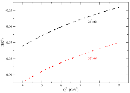
show a fishbone pattern due to lattice artifacts, as displayed in Fig. 1, making it difficult to extract physical vacuum polarization as a single-valued function of .
In contrast, the reflection averaging of Eq. (12) combined with an appropriate choice for produces the smooth curves displayed in Fig. 2 that retain a large number of usable values.

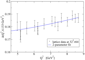
For the ensemble, which has the smaller lattice spacing, good fits are obtained with just 2 fit parameters. The fit function is Eq. (13) with parameters and . All other are set to zero because is sufficient to represent all of the lattice artifacts in this reflection-averaged data set. Figure 3 shows the resulting value for as a single red data point that appears on 6 different panels.
Panel (a) indicates that the result is not sensitive to changes in the light quark mass. Panel (b) shows insensitivity to our choice of ; the error bar grows if becomes too small because an agressive cut leaves too few data points in the fit.
Experience from decay phenomenology says GeV2 is required to avoid the OPE dangers described above, and panel (c) shows that these lattice results are consistent with that expectation. Results should be insensitive to if lattice artifacts are under control, and panel (d) verifies this for our data.
Equation (15) requires a subtraction point , and panel (e) shows the statistical variation obtained from choosing any single direction for instead of averaging over all equivalent options.
Panel (f) displays the systematic shift in that would come from truncating the perturbative expansion at a lower order. Although the red point does receive input from the estimated coefficient , our result is insensitive to its precise value.
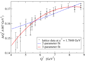
Results displayed in Fig. 3 are for the 3264 ensemble with GeV. We should perform a similar analysis for 2464 with GeV but two issues arise: (1) a two-parameter fit (Eq. (13) with and ) does not describe the data well, and (2) a three-parameter fit (Eq. (13) with , and ) allows a huge error bar for . The situation is displayed graphically in Fig. 4.


Unfortunately, we must conclude that a two-parameter fit is not sufficient for the coarse lattice, and that the statistical precision is not presently available to get from the 3-parameter fit.
4 Numerical result for
The analysis reported here gives
| (18) |
and running to the mass gives
| (19) |
which is in excellent agreement with results that use decay data from experiment for an alternate analysis of the same . In particular, the recent continuum FESR analysis of the 2013/14 corrected and updated ALEPH hadronic decay data arrived at [8]
| (20) |
Running our result in Eq. (18) to in the 5-flavor theory gives . For comparison, the FLAG Working Group result is [1] .
5 Summary
We have presented a new implementation to obtain from vacuum polarization at short distances. It avoids the danger of systematic errors that could arise in low-scale fits as a result of alternating-sign higher-dimension OPE contributions. Our method needs for many off-axis lattice directions. Our numerical results are competitive with the determination of from decay. In the future, we hope to use data from finer lattices since this will allow a study of the continuum limit.
Acknowledgments: This work was supported in part by NSERC of Canada.
References
- [1] S. Aoki et al., Eur. Phys. J. C 74, 2890 (2014) [arXiv:1310.8555 [hep-lat]].
- [2] E. Shintani et al. [JLQCD and TWQCD Collaborations], Phys. Rev. D 79, 074510 (2009) [arXiv:0807.0556 [hep-lat]].
- [3] E. Shintani, S. Aoki, H. Fukaya, S. Hashimoto, T. Kaneko, T. Onogi and N. Yamada, Phys. Rev. D 82, 074505 (2010) [Phys. Rev. D 89, 099903 (2014)] [arXiv:1002.0371 [hep-lat]].
- [4] E. Shintani, H. J. Kim, T. Blum and T. Izubuchi, PoS LATTICE 2013, 487 (2014).
- [5] G. Herdoiza, H. Horch, B. Jäger and H. Wittig, PoS LATTICE 2013, 444 (2014).
- [6] A. Francis, G. Herdoíza, H. Horch, B. Jäger, H. B. Meyer and H. Wittig, PoS LATTICE 2014, 163 (2014) [arXiv:1412.6934 [hep-lat]].
- [7] D. Boito, M. Golterman, K. Maltman, J. Osborne and S. Peris, Phys. Rev. D 91, no. 3, 034003 (2015) [arXiv:1410.3528 [hep-ph]].
- [8] D. Boito, M. Golterman, K. Maltman, J. Osborne and S. Peris, Nucl. Part. Phys. Proc. 260, 134 (2015) [arXiv:1410.8415 [hep-ph]].
- [9] P. A. Baikov, K. G. Chetyrkin and J. H. Kuhn, Phys. Rev. Lett. 101, 012002 (2008) [arXiv:0801.1821 [hep-ph]].
- [10] R. Arthur et al. [RBC and UKQCD Collaborations], Phys. Rev. D 87, 094514 (2013) [arXiv:1208.4412 [hep-lat]].