LATE COSMIC ACCELERATION IN A VECTOR–GAUSS-BONNET GRAVITY MODEL
Abstract
In this work we study a general vector-tensor model of dark energy with a Gauss-Bonnet term coupled to a vector field and without explicit potential terms. Considering a spatially flat FRW type universe and a vector field without spatial components, the cosmological evolution is analysed from the field equations of this model, considering two sets of parameters. In this context, we have shown that it is possible to obtain an accelerated expansion phase of the universe, since the equation state parameter satisfies the restriction (for suitable values of model parameters). Further, analytical expressions for the Hubble parameter , equation state parameter and the invariant scalar are obtained. We also find that the square of the speed of sound is negative for all values of redshift, therefore, the model presented here shows a sign of instability under small perturbations. We finally perform an analysis using observational data and we find that for the free parameter in the interval , at C.L. (and fixing and ), the model has a good fit to the data.
keywords:
Dark energy; Gauss-Bonnet coupling; Vector field.Received (Day Month Year)Revised (Day Month Year)
PACS Nos.: 95.36.+x, 98.80.-k, 04.50.Kd
1 Introduction
The existence of dark energy (DE) was postulated by two independent research groups in 1998 (High-z Supernova Search Team and Supernova Cosmology Project) to explain the regime of accelerated expansion of the current universe and became one of the greatest unsolved mysteries in physics; as a matter of fact, its origin from the fundamental point of view is still unknown [1, 2, 3, 4, 5]. This phenomenon has been supported also by the observed anisotropies in the CMB spectrum [6, 7] and the analysis of the large scale structures in the universe [8, 9, 10]. Many phenomenological and theoretical models have been considered in the last years to resolve the dark energy problem [11].
The natural candidate for dark energy is the cosmological constant [12, 13], conventionally associated with the energy of the vacuum with constant energy density and pressure, and an equation of state . Other proposals incorporate dynamical models of DE with scalar fields, which include quintessence, K-essence, tachyon, phantom, ghost condensates and dilaton [11, 14]. An alternative to dark energy is related to modified theories of gravity, [15, 16], or in its more general form [17, 18], in which dark energy emerges from the modification of geometry. Besides of scalar fields models of DE, in recent years some authors have considered another alternative about the nature of dark energy, suggesting the possibility that it could be described by a vector field [19, 20, 21, 22, 23, 24]. In this sense, we propose a vector-tensor model of dark energy with a Gauss-Bonnet (GB) term coupled to vector field and without explicit potential terms. With this proposal, we analyse a possible accelerated expansion phase of the universe in late times. In general, the GB term in four dimensions is known as a topological term, so the field equations are not influenced by it. However, when one considers the GB term coupled to the matter field, the field equations are modified. Further, the GB invariant has an important role in models with extra dimensions (see Ref. \refcitefarakos and references therein) and string theory. In string theory, the GB term arises when the tree-level effective action of the heterotic string is analysed [27, 28]. The GB term has been used for several authors in the context of inflation and dark energy models. A model with vector field coupled to GB invariant in a type Bianchi I universe was proposed in Ref. \refcitemota. Recently, in Ref. \refcitevalenzuela the authors have considered an inflation model with a cosmological vector field non-minimally coupled to gravity through the GB invariant. In the literature, usually the GB invariant has been used in models with scalar fields [29, 30, 31, 32, 33, 34, 35, 36, 37, 38, 39], and in these papers it is shown that the GB coupling term may be relevant for the explanation of accelerated expansion of the universe at late times.
This paper it is organized as follows: in section 2 we introduce the vector-tensor model with a GB term coupled to the vector field and the corresponding field equations are obtained. In section 3, we consider a flat FRW type universe and a vector field without spatial components, and from these considerations we analyse the cosmological evolution of this model. Section 4 is devoted to a statistical analysis of the model, by performing a fit of the single model parameter , to the observational data for . Finally, some conclusions are exposed in section 5.
2 The model
The most general action for the vector-Gauss-Bonnet dark energy model (without mater contributions) can be written as
| (1) | ||||
where , and are the Ricci tensor and the Ricci scalar, respectively, is a potential term, is the topological GB invariant, and free coupling constants (, , ) for each non-minimal coupling term are included. and are dimensionless, but the dimensions of are .
Different specific forms of this action have been studied, for instance, in Ref. \refciteharko, where dark energy is proposed to be represented by a massive vector field non-minimally coupled to gravity, but the Gauss-Bonnet invariant is not considered ( and in Eq. (1)); also, the authors of Ref. \refcitesadeghi considered a modified Gauss-Bonnet gravity model (, in Eq. (1)), in which inflation and late-time acceleration of the universe is realised.
The variation of the action (1) with respect to the metric tensor gives the field equations
| (2) |
where is the energy momentum tensor for the vector field and has the following form:
| (3) |
Each term is given by the following expressions (Eqs. (4)-(8)):
| (4) |
| (5) | ||||
| (6) | ||||
| (7) |
and
| (8) |
where , is an invariant scalar. For more details about the variation of the Gauss-Bonnet term, see [29].
On the other hand, the variation of the action with respect to , gives the equation of motion
| (9) |
3 Cosmological evolution
To analyse the cosmological evolution of the universe generated by the previous model and determine if it is possible to obtain a regime of accelerated expansion of the universe at late times, we regard the flat Robertson-Walker metric for a homogeneous and isotropic universe, given by
| (10) |
where is the scale factor. We consider that the vector field has only the temporal component, i. e. , which is in agreement with the observed isotropy and homogeneity of the universe.
Using the FRW metric in Eq. (9) and taking , we obtain
| (11) |
Here one can examine a number of interesting possibilities in order to simplify the problem under study; for instance, with , then , so that if then . In the present work, we have decided to study this case to analyse the cosmological evolution of such a model. Further details of this choice are discussed bellow.
From Eq. (2) and using the previous considerations, the Friedmann equations take the following form:
| (12) |
and
| (13) |
Here we have used . and are the dark energy and pressure density respectively of the vector field and are given by (using , )
| (14) |
and
| (15) | ||||
On the other hand, with the selected values for the coupling constants, the equation of motion (11) becomes
| (16) |
from which it is possible to obtain an analytical expression for the Hubble parameter, since the component of the vector field is easily decoupled (a similar result was obtained in Ref. \refciteharko). To facilitate the procedure, we carry out the change of variable ( is known as the e-folding variable). Then, Eq. (16) can be rewritten as
| (17) |
and the solution for this differential equation is
| (18) |
where is a integration constant and is the “Lambert W-Function” or “ProductLog” function. Using the initial condition, in (18), the integration constant is
| (19) |
Before continuing with the analysis of this model, we notice that by looking at Eq. (11), it is easy to see that another possible choice is . In this case, , so that if one gets . With these values for the coupling constants, the first term in Eq. (11) is neglected, and the Einstein’s tensor , arises in the action Eq. (1); also, from Eq. (11), the resulting differential equation has the solution
| (20) |
We stress that we checked the fact that the two exposed choices do produce very similar results, even though the solution shown in Eq. (20) is different compared to the Eq. (18).
Now, we consider the behavior of the equation of state parameter in order to determine if it is possible to obtain an accelerated expansion regime for the universe at late times. The equation of state parameter is given by
| (21) |
and using (18) and (19), we obtain
| (22) |
Fig. 1 shows the behavior of as a function of the redshift . The continuous line corresponds to the evolution of for , while the shaded region shows the result of for different possible values of within a ( C.L.) interval (see Sec. 4 for the details). We have considered here [42]. Also, the substitution has been realized.
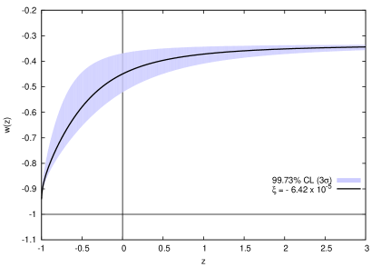
We can see in the Fig. 1 that it is possible to obtain a regime of accelerated expansion of the universe at late times for a wide range of values of the parameter (up to a CL), since the equation state parameter satisfy the restriction . This model behaves as a quintessence scalar field model and a phantom phase is not observed ( does not cross the barrier). Furthermore, the function satisfies the following limits
| (23) |
The second limit corresponds to a de Sitter solution ( is constant). In this case, the associated cosmological constant arises from the vector field. Finally,
| (24) |
In this last limit, the value of coupling constant is arbitrary and in this stage, the universe is dominated by the cosmological constant (de Sitter phase).
From Eq. (12) and using (14) and (19), we can obtain an expression for the invariant scalar , obtaining
| (25) |
where is an integration constant, which is given by the initial condition . The value of initial condition must be consistent with the restriction .
Choosing initial condition, , from (25) we obtain
| (26) |
Then, with (25) we plot the scalar invariant vs in Fig. 2. We again use the value for the free parameter (explanation provided in Sec. 4) and the corresponding allowed interval.
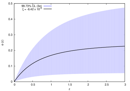
We see that the function is always positive for all redshift values.
In order to examine the stability of the model, we study the square of the speed of sound () as a function of the redshift. is given by [41]
| (27) |
where the prime means differentiation with respect to . From of Eqs. (14), (15), (18) and (25), Eq. (27) takes the explicit form
| (28) | ||||
and its evolution is depicted in Fig. 3, including the shaded band for the free parameter , as explained before.
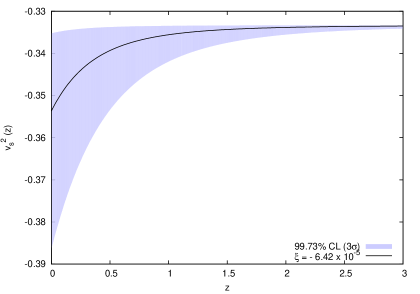
It is noted that is negative for all values of z, showing that the model presented here shows a sign of instability under small perturbations. This behavior does not depend of the initial condition , which is clear from Eqs. (14), (15) and (27) (one must take into account , and ). However, it is important to note that the positivity of is a necessary condition but is not enough to conclude that the model is stable [43].
4 Observational constraints using data
A simple but robust procedure to study models containing free parameters, is to perform a least-squares analysis (see Section 38 of Ref. \refcitepdg), comparing theoretical predictions from the model for a specific measurable quantity, with experimental or observational data. In this case, one can carry out such an analysis using the observational data of and the obtained result for the Hubble parameter given by Eq. (18) (or Eq. (20) -see bellow-), which depends explicitly on the only free parameter of the proposed model.
Here we consider data of the Hubble parameter for different values of the redshift, taken from Table I of Ref. \refciteDing, and consider the simple -function
| (29) |
where the sum runs up to , the total number of observed values; and are the observed and its corresponding uncertainty, respectively (as in [45]); and is the theoretical Hubble parameter, which depends on the redshift, , as well as on the free parameter , as expressed by (18).
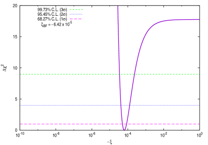
The main result of this analysis is presented in the form of the curve show in Fig. 4, where the quantity is plotted for an interesting interval of values of the free parameter . We found that the fit produces (for 28 d.o.f) when
| (30) |
In the figure, and according to [44], we also show the allowed intervals for the parameter up to (pink long–dashed line), (blue dotted line) and (green short–dashed line). The corresponding intervals can be seen in Table 4.
intervals for the parameter obtained by the data fit of the model to data. \topruleC.L. \colrule \botrule
Notice that our analysis excludes the case for which the GB term is not coupled to the vector field, , at more than C.L. Also, despite of the apparent narrowness of the curve in fig. 4 (note its log-scale of the horizontal axis), we obtained wide ranges for the values of the free parameter. In order to get even stronger constraints, one would need to have observational information with smaller uncertainties, or to use data of some other observables. For instance, one could use observational bounds on , as this parameter also appears explicitly in the theoretical prediction for , equations (18) and (19). Otherwise, PPN solar system constraints could be implemented.
In order to have a taste of the goodness of our fit, we compare the model prediction for using the best fit value obtained for the free parameter, , Eq. (30), with the data points from [45]. The resulting plot is shown in Fig. 5.
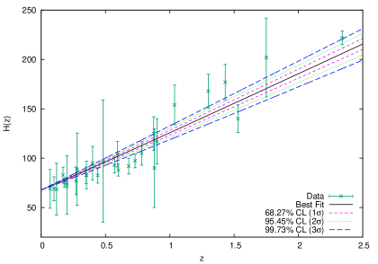
In the figure, data are plotted with their uncertainties and in addition to the Best Fit curve (continuous line), the (inside the blue long–dashed lines), (inside the green dotted lines) and (inside the pink short–dashed lines) bands are also depicted. Fig. 5 clearly shows that data points (plus uncertainties) are very well covered by the and even the bands, demonstrating that our model exhibits a good fit to the data. Once again, stronger bounds on observational data would certainly allow one to strengthen also the limits on the model.
Finally, as anticipated above, we have also performed the same kind of analysis for the other possible values of the parameters in Eq. (11), i.e. and . The fit to the observational data is very similar, giving a best fit value for the free parameter (with ). Although this value is slightly larger than (30), the evolution of given by Eq. (20) is almost equal to the one given by Eq (18). As a result, and in order to show this similarity, we compare the evolution of the equation of state, , as a function of the redshift. The result is exposed on Fig. 6.
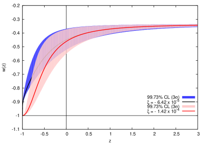
It is clear from the figure that the behaviour of is basically the same for the two sets of parameters (), from early times until present. In both of the cases, it remains valid that , as expected. On the other hand, even though there is a visible difference in the evolution of the two plot for , both of them go to , as expected, as well.
With this in hands, anyone could ask why we decided to work and exhibit one set of parameters over the other. In deed, the main reason is the fact that the case of () does not give an analytical solution for the invariant scalar , so making the case of () more interesting and easier to analyse.
5 Conclusions
The GB invariant coupled to the scalar fields has been widely used in the literature and it is shown that the GB coupling term may be relevant for the explanation of accelerated expansion of the universe at late times; it has also been considered in inflationary scenarios. Furthermore, the GB invariant has an important role in models with extra dimensions (braneworlds) and in string theory.
In this paper we have shown that it is possible to obtain an accelerated expansion phase of the universe for two different sets of values of the parameters and , from a general vector-tensor model given by Eq. (1), where a vector field coupled to GB term has been included. This conclusion is supported by the equation state parameter behavior shown in Fig. 1 (and Fig. 6), as well as Eq. (22), satisfying the restriction . Since does not cross barrier, then, a phantom phase isn’t observed. Moreover, when the equation state parameter and when , we have that . This latter case corresponds to a de Sitter solution ( is constant). In this case, the associated cosmological constant arises from the vector field. When (future) then , for any value of coupling constant and the universe in this case is dominated by the cosmological constant (see eqs. (23) and (24)). We have also obtained an analytical expression for the invariant scalar given by Eq. (25) and the initial condition was considered, which agrees with the restriction (see Fig. 2).
In order to examine the stability of the model, the square of the speed of sound () as a function of the redshift was analysed (see (28)) and we found that the square of the speed of sound is negative for all values of redshift; under this criterion, the model presented here shows a sign of instability under small perturbations (see Fig. 3). This behavior does not depend of the initial condition .
Finally, by performing a least-squares analysis with observational data of the Hubble parameter , we found that our model exhibits a good match to the data with a best fit given by for and (and for and ). As explained in Sec. 4, the analysis provides us with allowed regions for the free parameter (see Fig. 4 and Table 4), which are used to compute the important quantities along this article (, and ), as well as to perform a comparison with the data (Fig. 5). Accordingly, we can say that the vector-tensor model of dark energy considered in this work is a phenomenologically viable model. We stress out that, in a future work, the free parameters of the model (the coupling constant and initial value of the vector field) could be estimated by using additional restrictions, as for example, the PPN solar system constraints.
References
- [1] A. G. Riess et al. Astron. J 116, 1009 (1998).
- [2] A. G. Riess, Astron. J 117, 707 (1999).
- [3] S. Perlmutter et al, Nature 391, 51 (1998).
- [4] S. Perlmutter et al, [Supernova Cosmology Project Collaboration], Astrophys. J 517, 565 (1999).
- [5] P. Astier et al, Astron. Astrophys. J 447, 31 (2006).
- [6] D. N. Spergel et al, [WMAP Collaboration], Astrophys. J. Suppl. 148, 175 (2003).
- [7] D. N. Spergel et al, [WMAP Collaboration], Astrophys. J. Suppl. 170, 377 (2007).
- [8] M. Tegmark et al. [SDSS Collaboration], Phys. Rev. D 69, 103501 (2004).
- [9] K. Abazajian et al. [SDSS Collaboration], Astron. J 128, 502 (2004).
- [10] K. Abazajian et al. [SDSS Collaboration], Astron. J 129, 1755 (2005).
- [11] E. J. Copeland, M. Sami and Sh.Tsujikawa, Int. J. Mod. Phys. D 15, 1753 (2006).
- [12] S. Weinberg, Rev. Mod. Phys. 61, 1 (1989).
- [13] T. Padmanabhan, Phys. Rept. 380, 235 (2003).
- [14] F. Piazza and S. Tsujikawa, JCAP 07, 004 (2004).
- [15] S. Capozziello and M. De Laurentis, Phys. Rept. 509, 167 (2011).
- [16] S. Nojiri and S. D. Odintsov, Phys. Rept 505, 59 (2011).
- [17] M. De Laurentis, M. Paolella and S. Capozziello, Phys. Rev. D 91, 083531 (2015).
- [18] M. De Laurentis, Mod. Phys. Lett. A 30, 1550069 (2015).
- [19] V. V. Kiselev, Class. Quant. Grav. 21, 3323 (2004).
- [20] H. Wei and R.-Gen Cai, Phys. Rev. D 73, 083002 (2006).
- [21] T. S. Koivisto and D. F. Mota, JCAP 0808, 021 (2008).
- [22] J. B. Jimenez and A. L. Maroto, Phys. Rev. D 78, 063005 (2008).
- [23] J. B. Jimenez, R. Lazkoz and A. L. Maroto, Phys. Rev. D 80, 023004 (2009).
- [24] C. G. Böhmer and T. Harko, Eur. Phys. J. C 50, 423 (2007).
- [25] J. Sadeghi, M. R. Setare and A. Banijamali, Eur. Phys. J. C 64, 433 (2009).
- [26] K. Farakos and P. Pasipoularides, Phys. Rev. D 75, 024018 (2007).
- [27] C. G. Callan, Jr., E. J. Martinec, M. J. Perry and D. Friedan, Nucl. Phys. B 262, 593 (1985).
- [28] D. J. Gross and J. H. Sloan, Nucl. Phys. B 291, 41 (1987).
- [29] S. Nojiri, S. D. Odintsov and M. Sasaki, Phys. Rev. D 71, 123509 (2005).
- [30] G. Calcagni, S. Tsujikawa and M Sami, Class. Quant. Grav. 22, 3977 (2005).
- [31] I. P. Neupane and B. M. N. Carter, JCAP 0606, 004 (2006).
- [32] S. Tsujikawa and M. Sami, JCAP 0701, 006 (2007).
- [33] B. M. Leith and I. P. Neupane, JCAP 0705, 019 (2007).
- [34] T. Koivisto and D. F. Mota, Phys. Lett. B 644, 104 (2007).
- [35] S. Nojiri and S. D. Odintsov, Phys. Lett. B 631, 1 (2005).
- [36] K. Bamba, Z-K. Guo and N. Ohta, Prog. Theor. Phys. 118, 879 (2007).
- [37] G. Cognola, E. Elizalde, S. Nojiri, S. D. Odintsov and S. Zerbini, Phys. Rev. D 73, 084007 (2006).
- [38] S. Capozziello, A. N. Makarenko and S. D. Odintsov, Phys. Rev. D 87, 084037 (2013).
- [39] L. N. Granda and D. F. Jimenez, Phys. Rev. D 90, 123512 (2014).
- [40] J. C. Bueno-Sánchez and C. A. Valenzuela-Toledo, arXiv:1504.07983 [gr-qc].
- [41] P.J.E. Peebles, and B. Ratra, Rev. Mod. Phys. 75, 559 (2003).
- [42] Planck Collaboration, arXiv:1502.01589 [astro-ph.CO].
- [43] S. Ghaffari, M. H. Dehghani and A. Sheykhi, Phys. Rev. D 89, 123009 (2014).
- [44] K. A. Olive et al. [Particle Data Group Collaboration], Chin. Phys. C 38, 090001 (2014).
- [45] X. Ding, M. Biesiada, S. Cao, Z. Li and Z. H. Zhu, Astrophys. J. 803, no. 2, L22 (2015).