Global description of beta-minus decay in even-even nuclei with the axially-deformed Skyrme finite amplitude method

Abstract

We use the finite amplitude method for computing charge-changing Skyrme-QRPA transition strengths in axially-deformed nuclei together with a modern Skyrme energy-density functional to fit several previously unconstrained parameters in the charge-changing time-odd part of the functional. With the modified functional we then calculate rates of beta-minus decay for all medium-mass and heavy even-even nuclei between the valley of stability and the neutron drip line. We fit the Skyrme parameters to a limited set of beta-decay rates, a set of Gamow-Teller resonance energies, and a set of spin-dipole resonance energies, in both spherical and deformed nuclei. Comparison to available experimental beta-decay rates shows agreement at roughly the same level as in other global QRPA calculations. We estimate the uncertainty in our rates all the way to the neutron drip line through a construction that extrapolates the errors of known beta-decay rates in nuclei with intermediate $Q$ values to less stable isotopes with higher $Q$ values.

I Introduction

Beta-decay rates are an important ingredient in simulations of the astrophysical $r$-process. Because parts of the $r$-process path are still not accessible to experiment, it is up to theoretical models to produce approximate rates for many relevant neutron-rich isotopes. Models could also help resolve the issues raised by Ref. Mention et al. (2011), which argued that the flux of antineutrinos from nuclear reactors does not agree with the standard model. Ref. Hayes et al. (2014) pointed out that the discrepancy could be due to an overly simple treatment of first-forbidden beta decay in fission products.

Several schemes/methods for calculating beta-decay rates across almost the entire nuclear chart have been devised. They include the proton-neutron quasiparticle random phase approximation (pnQRPA) with a residual Gamow-Teller interaction Homma et al. (1996), gross theory Möller et al. (1997, 2003), semi-gross theory Nakata et al. (1997), the extended Thomas-Fermi plus Strutinsky integral (ETFSI) method Borzov and Goriely (2000), and artificial neural networks Costiris et al. (2009), and, very recently, the relativistic spherical pnQRPA Marketin et al. (2015). Full beta-decay tables for neutron-rich isotopes have been only published by Möller et al Möller et al. (1997, 2003) and Marketin et al Marketin et al. (2015).

Many other authors have applied more sophisticated and/or computationally intensive methods to smaller sets of nuclei, focusing on some of those important for the $r$ process. Recent examples of such work include a deformed pnQRPA computation with the Bonn-CD interaction of the decay of neutron-rich isotopes with $Z=36-43$ Fang et al. (2013), of isotopes of Zr and Mo Ni and Ren (2014a), and of isotopes of Kr and Sr Ni and Ren (2014b); similar calculations with Gogny interaction in the $N=82,126,184$ isotonic chains Martini et al. (2014); relativistic pnQRPA Niu et al. (2013) for $20\leq Z\leq 50$; and relativistic pnQRPA for $N\approx 50,82$ Nikšić et al. (2005).

Computational barriers have thus far prevented the production of a beta-decay table for the entire nuclear chart in a fully self-consistent Skyrme mean-field approach that allows deformation. Recently, however, we reported Mustonen et al. (2014) an implementation of the charge-changing finite amplitude method, which sidesteps the QRPA eigenvalue problem. We obtain beta-decay rates by directly computing the required sums and integrals over allowed final states of the response to charge-changing perturbations. We will soon make available a code called pnfam that implements the method.

We could proceed by choosing an existing density functional, interpreting it as a density-dependent effective interaction, and calculating beta-decay rates. If we were interested in, e.g., the effects of tensor terms discussed in Refs. Minato and Bai (2013) and De Donno et al. (2014), we could take them from already-parametrized functionals. Such a procedure would require some parameter fitting because pairing interactions and strengths, especially those associated with isoscalar pairing, are not usually specified alongside Skyrme particle-hole effective interactions. But that approach is still too limiting because not all Skyrme functionals can be consistently represented as effective interactions. In particular, the time-even and time-odd parts of the functional, which are related if the functional is the mean-field expectation value of a Hamiltonian, need not be related in more general constructions.

Our main goal here is to assess the ability of the Skyrme QRPA with deformation to predict $\beta^{-}$ decay, and to use existing data (decay rates and resonance energies) to constrain the isoscalar-pairing strength and the other time-odd coupling constants, which in the general energy-density functional (EDF) picture, are not fixed by fits to masses, precisely because they are independent of the time-even functional. In much of what follows, therefore, we will not assume that the functional results from mean-field theory with an interaction and so will have to fit a significant number of parameters. After presenting our methods and assessment, we display the (summarized) results of a a full table of beta-minus rates, computed with the pnFAM, for even-even nuclei in all medium-mass and heavy isotopic chains. We use a simple but apparently accurate model to quantify and extrapolate theoretical uncertainty.

This article is organized as follows: Section II is a brief overview of the theoretical background, and Section III details our computational approach and parameter-fitting procedures. In Section IV, we assess the quality of our results, comparing them to earlier work and to experimental data where available. Section V contains conclusions.

II Theoretical background

II.1 Finite amplitude method

The finite amplitude method (FAM), a formulation of the random-phase approximation that speeds the computation of nuclear response functions, was introduced in nuclear physics in Ref. Nakatsukasa et al. (2007). It was later generalized to the quasiparticle random phase approximation (QRPA) in Ref. Avogadro and Nakatsukasa (2011) and to the relativistic QRPA in Ref. Nikšić et al. (2013). In Ref. Mustonen et al. (2014) we applied the method to charge-exchange transitions, in particular allowed and first-forbidden beta decay.

The FAM solves equations for the amplitude of the linear response to a small but finite perturbation. As a result, the method does not directly yield the poles and residues of the response, which are the central objects in the matrix version of the QRPA. But if the goal of the computation is to get transition strength functions in a large model space the FAM can yield results in orders of magnitude less CPU time than matrix QRPA.

The FAM offers another advantage for beta decay: the weighted sums or integrals of transition strength can be expressed as contour integrals. This fact was first exploited by Hinohara et al. Hinohara et al. (2015), who evaluated the response at a relatively small number of complex frequencies to compute sum rules. In Ref. Mustonen et al. (2014) we used the idea to evaluate the more complicated beta-decay phase-space-weighted integrals, which are not analytic and contain interference terms between first-forbidden operators. With the FAM we can thus use typical supercomputer resources to calculate many observables in a large number of nuclei. We are able to extend systematic Skyrme parameter fitting from mean-field calculations to deformed QRPA calculations, at least in a preliminary way.

II.2 Model parameters and fitting targets

Our starting point in the particle-hole channel is a generic Skyrme EDF:

$$\mathcal{E}=\sum_{t=0,1}\sum_{t_{3}=-t}^{+t}\int\mathrm{d}\mathbf{r}\,\bm{\left(}\mathcal{H}_{tt_{3}}^{\mathrm{even}}(\mathbf{r})+\mathcal{H}_{tt_{3}}^{\mathrm{odd}}(\mathbf{r})\bm{}\,.$$ (1)

Here $\mathcal{H}_{tt_{3}}^{\mathrm{even}}$ contains products of time-even local densities only, with coefficients fixed by fitting to masses and perhaps a few other quantities, and $\mathcal{H}_{tt_{3}}^{\mathrm{odd}}$ is given by

$$\mathcal{H}_{tt_{3}}^{\mathrm{odd}}(\mathbf{r}) \equiv C_{t}^{s}[\rho_{00}]\mathbf{s}_{tt_{3}}^{2}+C_{t}^{\Delta s}\mathbf{s}_{tt_{3}}\cdot\bm{\nabla}^{2}\mathbf{s}_{tt_{3}}+C_{t}^{j}\mathbf{j}_{tt_{3}}^{2}$$ (2)

$$+C_{t}^{T}\mathbf{s}_{tt_{3}}\cdot\mathbf{T}_{tt_{3}}+C_{t}^{s\nabla j}\mathbf{s}_{tt_{3}}\cdot\bm{\nabla}\times\mathbf{j}_{tt_{3}}$$

$$+C_{t}^{F}\mathbf{s}_{tt_{3}}\cdot\mathbf{F}_{tt_{3}}+C_{t}^{\nabla s}\left(\bm{\nabla}\cdot\mathbf{s}_{tt_{3}}\right)^{2}\,,$$

with the spin density $\mathbf{s}_{tt_{3}}$, the current density $\mathbf{j}_{tt_{3}}$, the spin-kinetic density $\mathbf{T}_{tt_{3}}$, and the tensor-kinetic density $\mathbf{F}_{tt_{3}}$ defined e.g. in Ref. Perlińska et al. (2004). If one requires the functional to be the mean-field expectation value of a Skyrme interaction, EDF coupling constants are completely determined by the (fewer) parameters that specify the interaction, as discussed in Refs. Perlińska et al. (2004); Bender et al. (2002) and mentioned above. In this work, we adopt the view that the effective “interaction” comes from the energy-density functional rather than the other way around. Consequently we are free to fit all the time-odd coupling constants without spoiling the mass fits generated the time-even couplings. We do, however, adopt the values obtained from the Skyrme parametrization as our starting point for the fits, unless we note otherwise.

The subset $\{C^{s}_{1},C^{T}_{1},C^{F}_{1}\}$ of time-odd coupling constants maps directly to the parameters of Landau-Migdal interaction for infinite homogeneous nuclear matter with tensor terms Bäckman et al. (1979). In that sense, these couplings are intimately related to the bulk properties of the nuclear matter. The constant $C^{F}_{1}$ is purely tensor in character, and it determines the tensor term in the Landau-Migdal interaction. The spin-density coupling constant $C^{s}_{1}$ strongly affects the Gamow-Teller strength distribution and can be fit to the locations of Gamow-Teller resonances Bender et al. (2002). The last term $C^{T}_{1}$ maps to a linear combination of the Landau parameters of both the tensor term and a term that depends on the scattering angle of the Laundau-Migdal quasiparticles.

Two other parameters have a large effect in the QRPA: the strengths of the residual particle-particle (or pairing) interaction between protons and neutrons,

$$V_{\mathrm{pp}}=\left(V_{0}\hat{\Pi}_{T=0}+V_{1}\hat{\Pi}_{T=1}\right)\left(1-\alpha\frac{\rho_{00}(\mathbf{r})}{\rho_{c}}\right)\delta(\mathbf{r}),$$ (3)

where $\rho_{c}=0.16$ fm^-3 is the saturation density of nuclear matter and $\alpha\in[0,1]$ controls the pairing density-dependence (throughout this work we use mixed pairing, i.e. $\alpha=0.5$). The isovector ($T=1$) proton-neutron pairing mainly affects Fermi beta decay, which plays almost no role in heavy nuclei; we simply set its strength $V_{1}$ to be the average of the neutron-neutron and proton-proton pairing strengths (both fixed in the HFB part of the calculation). The isoscalar ($T=0$) pairing is a different story; it has a strong effect on Gamow-Teller decay, and determining a reasonable value for its strength is a common issue in single and double beta decay computations. The HFB mean field is independent of the $T=0$ pairing term as long as explicit proton-neutron mixing is neglected. We are thus free to fit $V_{0}$ in the QRPA.

We include three types of observables in our fitting procedure: Gamow-Teller resonance energies, spin-dipole resonance energies, and total beta decay rates, all in both spherical and deformed isotopes. Although we pick several sets of target nuclei for fitting the decay half-lives, each set includes a large range of mass values so that our fits can be global. To assess the success of the fits and to compare them to earlier work in very different models, we also compute the following metrics for beta-decay tables, as laid out e.g. in Möller et al. (1997, 2003): the residual of each computed $\lg t$ value (where $t$ is the half-life and the logarithm is 10-based),

$$r=\lg\left(\frac{t_{\textrm{th.}}}{t_{\textrm{exp.}}}\right),$$ (4)

the average of the residuals,

$$M_{r}=\frac{1}{n}\sum_{i=1}^{n}r_{i},$$ (5)

(where we’ve used an index $i$ to indicate that there is an $r$ for every nucleus) and the standard deviation of the residuals around the average,

$$\sigma_{r}=\sqrt{\frac{1}{n}\sum_{i=1}^{n}\bigl{[}(r_{i}-M_{r}\bigr{]}^{2}}.$$ (6)

Ref. Costiris et al. (2009) contains an excellent compilation of these quantities.

II.3 Uncertainty analysis

As theoretical approaches grow more sophisticated, the analysis of theoretical uncertainty is growing in importance. Here we attempt to provide reasonable estimates for the uncertainty in our predicted half-lives, particularly in isotopes that are too short-lived to allow measurement.

The standard prescription for assigning a theoretical (statistical) uncertainty $\Delta\mathcal{O}$ to a computed observable $\mathcal{O}$ is Dobaczewski et al. (2014)

$$\Delta\mathcal{O}=\sqrt{\sum_{ab}\frac{\partial\mathcal{O}}{\partial x_{a}}\bigg{|}_{x=x_{0}}C_{ab}\frac{\partial\mathcal{O}}{\partial x_{b}}\bigg{|}_{x=x_{0}}},$$ (7)

where $C$ is the covariance matrix

$$C=(J^{T}J)^{-1}$$ (8)

and $x=(x_{1},\ldots,x_{N_{x}})$ are the $N_{x}$ parameters of the model. The partial derivatives of all the observables $\{\mathcal{O}_{a}\}$ with respect to all the parameters evaluated at the result of the fit $x_{0}$ form the Jacobian $J$:

$$J_{ab}=\frac{\partial\mathcal{O}_{a}}{\partial x_{b}}\bigg{|}_{x=x_{0}}.$$ (9)

When not analytically accessible, the needed partial derivatives can be estimated through finite central differences. (In general, the theoretical uncertainty related to the Jacobian must be supplemented by numerical and experimental uncertainties. We have assumed that the theoretical uncertainty is much larger than the other two, which we therefore neglect.)

To use Eq. (7) to assign an uncertainty to every beta-decay rate in our table, we would need to evaluate the Jacobian in Eq. (9) for (the logarithms of) all the half-lives $t$ in our table. Unfortunately, the required $2N_{x}$ full decay-table computations are still not possible in a reasonable amount of computer time, even with the efficiency of the FAM. We therefore attempt to gauge the uncertainties and their $Q$ dependence in a more naïve way. We construct a simple few-parameter model for the uncertainties that we can then fit to the observed differences between our numerical results and known experimental values. The resulting approach is agnostic about how the decay is actually calculated; it treats the nuclear model as a black box that produces predictions for $Q$ values and beta-decay rates. It does, however, make several assumptions about both the calculated and experimental strength distributions that are only approximately correct.

The first assumption is that the final states that contribute significantly to a decay rate lie not too far from the ground state in a relatively small window of excitation energy, so that we can reasonably approximate them, again either in our calculation or in the real world, by one effective state with an effective $Q$ value $q_{\mathrm{eff}}$ (that is not too different from the ground-state $Q$ value):

$$q_{\mathrm{eff}}=\frac{\sum_{k}C_{k}f_{k}(q_{k}+1,Z_{f})\,q_{k}}{\sum_{k}C_{k}f_{k}(q_{k}+1,Z_{f})}\,.$$ (10)

Here $C_{k}$ is the standard integrated shape function for the transition to the final state $k$ — for an allowed state decay this is simply the transition strength, and for a non-unique forbidden decay it encapsulates several terms — and $f_{k}$ is the usual allowed phase-space integral. The quantity $q_{k}$ is the $Q$ value of the decay to the state $k$ divided by $m_{e}c^{2}$, and $Z_{f}$ is the charge of the daughter nucleus.

With these definitions, we can proceed to define an effective shape factor $C_{\mathrm{eff}}$ as

$$t=\frac{\kappa}{\sum_{k}C_{k}f(q_{k}+1,Z_{f})}=\frac{\kappa}{C_{\mathrm{eff}}f(q_{\mathrm{eff}}+1,Z_{f})}.$$ (11)

The $C_{k}$ depend on the $q_{k}$ for forbidden transitions, but the dependence is weak compared to that of the corresponding phase-space integral, and so we neglect it in our effective shape factor.

All these definitions can be made independently for the experimental strength distribution and the theoretical one. The quantity we wish to understand is the ratio $r$ of the theoretical and experimental lifetimes:

$$\begin{split}r=&\lg\frac{t_{\textrm{th}}}{t_{\textrm{exp}}}\\ =&\lg\frac{C_{\textrm{eff}}^{\mathrm{exp}}}{C_{\textrm{eff}}^{\textrm{th}}}\\ &+\lg f(q_{\textrm{eff}}^{\textrm{exp}}+1,Z_{f})-\lg f(q_{\textrm{eff}}^{\textrm{th}}+1,Z_{f})\,,\end{split}$$ (12)

where the meanings of $q_{\textrm{eff}}^{\textrm{exp}}$ and $q_{\textrm{eff}}^{\textrm{th}}$ and the corresponding quantities $C_{\textrm{eff}}^{\mathrm{exp}}$ and $C_{\textrm{eff}}^{\textrm{th}}$ should be clear. We omit the nucleus index $i$ in them for brevity. Because the phase space grows quickly with decay energy, the effective $Q$ values will usually be close to ground-state-to-ground-state $Q$ value. We therefore expand both logarithms in Eq. (12) of the phase-space factors about the theoretical ground-state-to-ground-state $Q$ value $q_{\textrm{g.s.}}^{\textrm{th}}$ to first order in $q$:

$$\begin{split}\lg f(q+1,Z_{f})\approx&\lg f(q^{\textrm{th}}_{\textrm{g.s.}}+1,Z_{f})\\ &+\frac{d\lg f(q+1,Z_{f})}{dq}\biggr{|}_{q=q^{\textrm{th}}_{\textrm{g.s.}}}\cdot(q-q^{\textrm{th}}_{\textrm{g.s.}})\\ =&\lg f(q^{\textrm{th}}_{\textrm{g.s.}}+1,Z_{f})\\ &+\frac{f^{\prime}(q^{\textrm{th}}_{\textrm{g.s.}}+1,Z_{f})}{f(q^{\textrm{th}}_{\textrm{g.s.}}+1,Z_{f})}\cdot\frac{q-q^{\textrm{th}}_{\textrm{g.s.}}}{\ln 10}.\end{split}$$ (13)

This approximation is best when the $Q$ value is high, because the curvature of $\lg f(q+1,Z_{f})$ is small at high $q$. For $Q$ values lower than about 2–3 MeV the first-order approximation is poor, so we exclude such data points from our analysis.

Replacing the two logarithms in Eq. (12) by the first-order expressions, we find that several terms cancel in the difference, so that

$$\begin{split}r\approx&\lg\frac{C_{\textrm{eff}}^{\textrm{exp}}}{C_{\textrm{eff}}^{\textrm{th}}}\\ &+\frac{f^{\prime}(q^{\textrm{th}}_{\textrm{g.s.}}+1,Z_{f})}{f(q^{\textrm{th}}_{\textrm{g.s.}}+1,Z_{f})}\cdot\frac{q_{\textrm{eff}}^{\mathrm{exp}}-q_{\textrm{eff}}^{\textrm{th}}}{\ln 10}\,.\end{split}$$ (14)

We now make another set of assumptions, this time about the distribution of the errors in the theoretical values: First, we assume that the relative error in the effective shape factor is normally distributed with a slight systematic component. That is, we assume that for each nucleus, we have

$$\lg\frac{C^{\textrm{exp}}_{\textrm{eff}}}{C^{\textrm{th}}_{\textrm{eff}}}=c+\delta c,$$ (15)

where $c$ is a constant, independent of the nucleus in which the decay occurs, that captures the systematic error and the set of all nucleus-dependent $\delta c$’s is normally distributed with standard deviation $\Delta c$, which is a measure of statistical error that is independent of decay energy. Similarly, we assume that the errors in the theoretical effective $Q$ value follow a normal distribution, so that

$$\frac{q_{\textrm{eff}}^{\textrm{exp}}-q_{\textrm{eff}}^{\textrm{th}}}{\ln 10}=q+\delta q,$$ (16)

where $q$ is now a nucleus-independent systematic error in the effective $Q$ value and the set of $\delta q$’s (again, one for each nucleus) is normally distributed around zero with the standard deviation $\Delta q$ that represents statistical error, again independent of $Q$. (Both $q$ and $\delta q$ are expressed in units of $m_{e}c^{2}$, and the factor $1/\ln 10$ is absorbed into $q$ and $\delta q$ for convenience.) Finally, we assume that the errors $\delta q$ and $\delta c$ are independent.

With these assumptions, we then have

$$r=c+\frac{f^{\prime}(q^{\textrm{th}}_{\textrm{g.s.}}+1,Z_{f})}{f(q^{\textrm{th}}_{\textrm{g.s.}}+1,Z_{f})}\cdot q+\delta r,$$ (17)

where $\delta r$ is a random error, the set of which must be normally distributed at each $q^{\textrm{g.s.}}_{\textrm{th}}$ with width

$$\Delta r(q^{\textrm{th}}_{\textrm{g.s.}})^{2}={\Delta c^{2}+\biggl{(}\frac{f^{\prime}(q^{\textrm{th}}_{\textrm{g.s.}}+1,Z_{f})}{f(q^{\textrm{th}}_{\textrm{g.s.}}+1,Z_{f})}\biggr{)}^{2}\Delta q^{2}}.$$ (18)

We can now use Eqs. (17) and (18) to determine the values of $c$, $q$, $\Delta c$, and $\Delta q$. We obtain the first two through a fit to Eq. (17), which expresses $r_{i}$ as a function of $f^{\prime}/f$ (and thus of $q_{\textrm{g.s.}}^{\textrm{th}}$), with the set of ratios $r_{i}$ given by our calculations (and experiment) and $\delta r_{i}$ set to zero. Finally, we insert the fit values of $c$ and $q$ into the square of Eq. (17), which then expresses $\delta r_{i}^{2}$ as a function of $(f^{\prime}/f)^{2}$, and determine the values of $\Delta c$ and $\Delta q$ by requiring that the line for $\Delta r(q_{\textrm{g.s.}}^{\textrm{th}})^{2}$ as a function of $(f^{\prime}/f)^{2}$ that expresses Eq. (18) goes through the middle of the data, with as many points below $\Delta r^{2}$ as above it. A second least squares fit of $\Delta c$ and $\Delta q$ in the right hand side of Eq. (18) to the set of $\delta r_{i}^{2}$’s accomplishes the task nicely. The explicitly $Q$-dependent $\Delta r$ can then be extrapolated to large $Q$ values where there are no data.

For both fits, in practice, we only include data points with $Q\geq 3$ MeV and exclude any data points with $|r_{i}|>4$ as obvious outliers. We also adopt the Primakoff-Rosen approximation Primakoff and Rosen (1959) for the phase-space integral in the uncertainty model, making the expression $f^{\prime}/f$ a simple ratio of two polynomials, independent of $Z_{f}$:

$$\frac{f^{\prime}(x,Z_{f})}{f(x,Z_{f})}\approx\frac{5x^{4}-20x+15}{x^{5}-10x^{2}+15x-6}.$$ (19)

Once the four parameters of the uncertainty model have been determined, the uncertainties of the theoretical predictions are obtained the inverse relation of (4)

$$t_{\mathrm{exp}}=t_{\mathrm{th}}\cdot 10^{r}$$ (20)

with

$$r=r(q^{\textrm{th}}_{\textrm{g.s.}})\pm\Delta r(q^{\textrm{th}}_{\textrm{g.s.}}).$$ (21)

III Skyrme functional and computational method

Figure 1: The differences between computed and experimental $Q$ values, with SkO’ (top) and with SV-min (bottom). The insets show the distribution of differences. The errors in our computed $Q$ values follow a normal distribution with an average of $0.154$ MeV and a standard deviation of $0.576$ MeV, with no noticeable bias when moving to higher $Q$ values.

set	GT resonances	SD resonances	beta-decay half-lives
A	208Pb, 112Sn, 76Ge, 130Te, 90Zr, 48Ca	none	48Ar, 60Cr, 72Ni, 82Zn, 92Kr, 102Sr, 114Ru, 126Cd, 134Sn, 148Ba
B	same as A	none	52Ti, 74Zn, 92Sr, 114Pd, 134Te, 156Sm, 180Yb, 200Pt, 226Rn, 242U
C	same as A	none	52Ti, 72Ni, 92Sr, 114Ru, 134Te,156Nd, 180Yb, 204Pt, 226Rn, 242U
D	those of A and 150Nd	none	58Ti, 78Zn, 98Kr, 126Cd, 152Ce,166Gd, 204Pt
E	same as D	90Zr, 208Pb	58Ti, 78Zn, 98Kr, 126Cd, 152Ce, 166Gd, 226Rn

Table 1: The sets of fitting targets used in this work. The beta-decay half-lives in set A range from $0.069$ s (¹⁰²Sr) to $1.84$ s (⁹²Kr), in set B from $95.6$ s (⁷⁴Zn) to $45360$ s (²⁰⁰Pt), in set C from $0.54$ s (¹¹⁴Ru) to $9399.6$ s (⁹²Sr), and in set E from $0.046$ s (⁹⁸Kr) to $444$ s (²²⁶Rn). The nuclei selected for fitting the beta-decay half-lives in sets D and E all exhibit an excitation spectrum clearly associated with either a spherical or a well-deformed shape; set E only consists of open-shell nuclei. The experimental Gamow-Teller resonance energies are from Refs. Akimune et al. (1995); Anderson et al. (1985); Madey et al. (1989); Pham et al. (1995); Wakasa et al. (1997), the spin-dipole resonance energies from Refs. Yako et al. (2006); Wakasa et al. (2012), and the half-lifes from Ref. ens (2014).

The first step in our computational procedure is the construction of ground states in the doubly-even mother nucleus with hfbtho, a well-established HFB solver working in a (transformed) harmonic-oscillator basis Stoitsov et al. (2013). We cut off the single-particle space at $60$ MeV to avoid divergences from our zero-range pairing. For each nucleus, we search for a prolate, an oblate, and a spherical solution, and take the most bound of these to be the ground state.

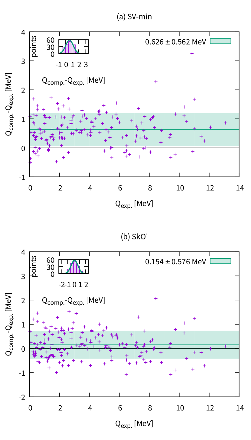
Because the beta-decay rates are very sensitive to the $Q$ value of the decay, we look for a modern Skyrme functional that reproduces $Q$ values well. Because we don’t explicitly treat odd nuclei, we use the prescription of Ref. Engel et al. (1999) to approximate the $Q$ value; we have checked the prescription against odd-A calculations in the equal filling approximation, and the two procedures generally agree to within about 0.5 MeV. Of the several functionals we examine, SkO’ Reinhard et al. (1999) (with the strengths of proton-proton and neutron-neutron pairing fit to the experimental pairing gaps of ten isotopes picked in a wide mass range $50\leq A\leq 230$) does the best job with $Q$ values, producing errors for ground-state-to-ground-state $Q$ values that are normally distributed, with an average systematic error of $0.154$ MeV and statistical error of $0.576$ MeV. Figure 1 compares the $Q$ values produced by SkO’ with those of the next best functional, SV-min.

To compute beta-decay rates and resonance energies we use the code pnfam, an implementation of the charge-changing finite amplitude method presented in Mustonen et al. (2014). Built to work together with hfbtho, pnfam allows us to compute properties of axial deformed nuclei, including both allowed and first-forbidden beta decay.

We obtain our most robust fits by fixing all but two of the time-odd coupling constants of the functional at values implied by its interpretation as an interaction. (The mapping of the Skyrme coupling constants to the energy-density functional coupling constants is explicitly discussed in Refs. Perlińska et al. (2004); Bender et al. (2002).) The exceptions are $C^{s}_{1}$ and $C^{\Delta s}_{1}$. We set the latter to zero to avoid known finite-size instabilities Schunck et al. (2010) which, in the case of hfbtho and pnfam, manifest themselves as divergences in the iterative solution. That leaves $C^{s}_{1}$, which, along with the isoscalar pairing strength $V_{0}$, we fit to a set of Gamow-Teller resonance energies, spin-dipole resonance energies, and beta-decay rates selected from a wide mass range with no particular region favored. We use the code pounders, based on a derivative-free algorithm Munson et al. (2012) designed for optimizing computer-time-consuming penalty functions, to efficiently minimize the weighted the sum of the least squares, simultaneously fitting both parameters. We take $C^{s}_{1}$ to be independent of the density and $V_{0}$ to have the same density dependence as the proton and neutron pairing. The axial-vector coupling constant $g_{\textrm{A}}$ is known to be quenched in nuclei, but the source and magnitude of the quenching is an open problem; a variety of very different values for an effective $g_{\textrm{A}}$ have been used. For lack of a better prescription, we use the commonly adopted quenched value $g_{\textrm{A}}=1.0$ in the Gamow-Teller channel, while applying no quenching in in the first-forbidden channels. We weight the three types of observables — two kinds of energies and a rate — in the least-squares fit so as to approximately normalize the total penalty function $\chi^{2}$ to the number of degrees of freedom, following the recommendation in Ref. Dobaczewski et al. (2014). We assume that the theoretical error dominates the experimental error, and thus assign equal weight to observable of the same type. We select these weights based on how well the different observables are reproduced in an initial test fit, so that each type of observable is approximately equally weighted in the actual fit. Typical fits then take 10—20 thousand CPU hours, and we use XSEDE supercomputers Towns et al. (2014) to carry them out.

Following the fit, we proceed to compute the beta-decay rates of all even-even neutron-rich nuclei with $28\leq Z\leq 110$, $A\geq 50$, all the way to the neutron drip line, omitting just a few very stable isotopes for which the $Q$ value is negative in our HFB calculations.

Figure 2: Reproduction of target data in those of our fits that use the target set E. The four-parameter fits 3A and 3B yield almost the same results as the two-parameter fits 1D and 1E, with only a small decrease in the penalty function.

IV Results and discussion

IV.1 Fit results

Figure 3: Comparison of the mean and standard deviation of the $\lg t$ values in our fits with those of previous work. The labels for our fits correspond to those of Table 1. The results from prior work are contained in Möller et al. (2003) (Mö), Homma et al. (1996) (Ho), Nakata et al. (1997) (Na), Costiris et al. (2009) (Co), and Marketin et al. (2015) (Ma). Only even-even isotopes are considered.

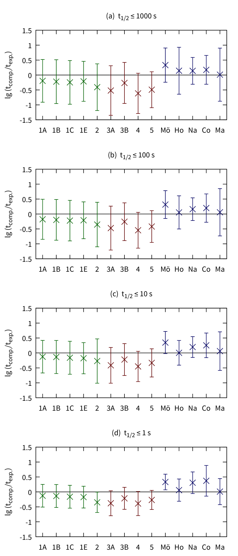
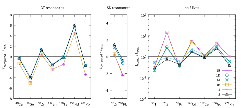
To assess how sensitive our fit is to the set of target beta-decay rates and resonance energies, we repeat the process with four sets of rates, summarized in Table 1. Each of these sets spans a large range of masses. Set A contains beta-decay isotopes with relatively short half-lives only, set B relatively long half-lives only, and set C a wide range of half-lives. (Short half-lives should be less sensitive to details in nuclear structure). Set D contains only nuclei that are known to be rather rigid, with an excitation spectrum characteristic of a spherical or a well-deformed nucleus. (The QRPA, which is based on a single mean field, should work best in rigid nuclei). In set E, we include only open-shell rigid nuclei (for which isoscalar pairing should be most effective), swapping out ²⁰⁴Pt for ²²⁶Rn, and including two spin-dipole resonances. Figure 2 shows the quality of the fits for set E both with computed (1D) and experimental (1E) $Q$ values (see Table 3 for definitions of the number-letter combinations). The two procedures yield very similar results. The comparison in Fig. 3, which shows the results of the two-parameter fits (along with those of more-parameter fits discussed shortly) when the resulting functionals are applied to the set of all measured even-even $\beta^{-}$-decay half-lives, shows that all these two-parameter fits (1A through 1E) yield the same level of predictive accuracy.

Can we do better by including some of the other time-odd coupling constants in our fit? To find out, we refit the four-parameter set $\{V_{0},C^{s}_{1},C^{T}_{1},C^{F}_{1}\}$, which determines the Landau parameters $\{g_{0}^{\prime},g_{1}^{\prime},h_{0}^{\prime}\}$ and thus allows us to incorporate infinite-nuclear-matter stability conditions Bäckman et al. (1979) as constraints. The parameter $C^{F}_{1}$ introduces a time-odd tensor term that is not present in the two-parameter fits. The result, however, improves the description of the fitting targets only marginally, as the points labeled 3A and 3B in Fig. 2 show, and actually worsens the agreement with half-life measurements overall (as Fig. 3 shows). The situation gets even worse when we use the results of this fit as a starting point to fit three more time-odd coupling constants, $\{C^{j}_{1},C^{\nabla j},C^{\nabla s}\}$ (fit 4). Then the beta-decay rates to which we fit are reproduced better, but the agreement with all measured rates deteriorates.

Improvement in the fitting targets accompanying a deterioration in overall agreement with data is a symptom of overfitting. To better understand why this happens, we evaluate the Jacobian matrix (9) at the parameter values produced by the two-parameter fit 1E. The Jacobian appears in Table 2, with the values of the coupling constants in natural units following the prescription of Ref. Kortelainen et al. (2010) and the natural scale of isoscalar pairing taken to be the strength of isovector pairing. A clear column structure appears in both the resonance energies and the half-lives, signaling that the members of each individual set move largely in unison when the parameters are varied. Thus there are essentially just two meaningful degrees of freedom that we can expect to fix with this experimental data: $V_{0}$ and $C^{s}_{1}$.

To see this in more detail, we carry out a singular value decomposition of the Jacobian. The largest singular value, $122.53$, corresponds to a vector pointing nearly in the direction of $C^{s}_{1}$ in parameter space, and the second largest, $10.85$, to a vector pointing nearly in the direction of $V_{0}$. The third largest value, $1.648$, is almost two orders of magnitude smaller than the largest, and corresponds mostly to $C^{T}_{1}$, with many other directions mixed in. The charge-changing data we have available — Gamow-Teller and spin-dipole resonances, and half-lives — are not enough to reasonably constrain more than the parameters $V_{0}$ and $C^{s}_{1}$ in our initial fit.

Figure 3, besides containing the results of our fits, contains results from other work: Refs. Homma et al. (1996); Nakata et al. (1997); Costiris et al. (2009) and Marketin et al. (2015). Of all the these computations, the one by Homma et al. Homma et al. (1996) seems to best reproduce the known $\beta^{-}$ half-lives, even though it neglects non-unique first-forbidden decay and uses simple separable interactions. As Figure 4 shows, in our computation the non-unique $1^{-}$ contribution is quite important (even dominant) in many experimentally inaccessible nuclei, so it is far from clear how the various calculations will fare with data in the future. In any event, the most striking fact is that all the computations manage to existing data at roughly the same level of precision. It may not be possible to do much better without moving beyond Skyrme QRPA, at least while using a global parameter set as we have done here.

IV.2 Extrapolation to neutron-rich isotopes

Figure 4 displays the relative contribution to the decay rate from each multipole. Except in the immediate vicinity of the valley of stability, the changes appear quite gradual as a function of $Z$ and $N$. In nuclei with large $Q$ values, the details of single-particle structure are less important than in isotopes for which transitions to only a few low-energy states are possible.

$\mathcal{O}$	$d\mathcal{O}/dC^{s}_{1}$	$d\mathcal{O}/dV_{0}$	$d\mathcal{O}/dC^{F}_{1}$	$d\mathcal{O}/dC^{T}_{1}$	$d\mathcal{O}/dC^{\nabla s}_{1}$	$d\mathcal{O}/dC^{\Delta s}_{1}$	$d\mathcal{O}/dC^{j}_{1}$	$d\mathcal{O}/dC^{\nabla j}_{1}$
208Pb $E_{\textrm{GTR}}$	57.261	-0.000	2.434	5.869	0.429	-1.002	0.000	0.143
112Sn $E_{\textrm{GTR}}$	29.498	-1.032	1.432	2.863	0.286	-0.573	0.000	0.000
76Ge $E_{\textrm{GTR}}$	45.115	-7.225	2.004	4.295	0.429	-1.145	0.000	0.000
130Te $E_{\textrm{GTR}}$	53.790	-3.096	2.434	5.297	0.429	-1.002	0.143	0.000
90Zr $E_{\textrm{GTR}}$	29.498	-1.032	1.288	2.720	0.429	-1.002	-0.143	0.143
48Ca $E_{\textrm{GTR}}$	32.968	-0.000	1.432	3.149	0.573	-1.288	0.000	0.000
208Pb $E_{\textrm{SDR}}$	52.055	-0.000	2.291	4.008	0.286	-1.575	-0.143	-0.143
90Zr $E_{\textrm{SDR}}$	29.498	-0.000	1.575	2.004	0.286	-1.432	-0.286	-0.143
58Ti $\lg t$	4.749	-4.318	0.203	0.445	0.045	-0.109	-0.011	-0.002
78Zn $\lg t$	6.889	-2.922	0.256	0.589	0.164	-0.382	0.253	-0.025
98Kr $\lg t$	5.410	-3.252	0.265	0.559	0.050	-0.116	-0.012	-0.003
126Cd $\lg t$	5.583	-4.641	0.252	0.496	0.017	-0.050	0.001	0.007
152Ce $\lg t$	5.409	-2.474	0.293	0.540	0.051	-0.120	0.003	-0.009
166Gd $\lg t$	5.081	-2.924	0.250	0.497	0.035	-0.132	-0.007	-0.010
204Pt $\lg t$	3.755	-3.340	-0.015	0.160	-0.018	-0.316	-0.076	0.026

Table 2: The Jacobian matrix, evaluated at the result of the two-parameter fit 1E. All parameters except for the strength of isoscalar pairing are expressed in natural units. The strength of isoscalar pairing has been scaled by the strength of isovector pairing. The derivatives of the $\lg t$ values are hence dimensionless and those of the resonance energies are in the units of MeV.

fit	starting point	target set	$Q$ values	fitted parameters
1A	SkO’	A	comp.	$V_{0}=-173.176$, $C^{s}_{1}=128.279$
1B	SkO’	B	comp.	$V_{0}=-176.614$, $C^{s}_{1}=133.038$
1C	SkO’	C	comp.	$V_{0}=-176.097$, $C^{s}_{1}=126.966$
1D	SkO’	E	comp.	$V_{0}=-209.384$, $C^{s}_{1}=129.297$
1E	SkO’	E	exp.	$V_{0}=-159.397$, $C^{s}_{1}=99.8479$
2	SV-min	D	comp.	$V_{0}=-165.567$, $C^{s}_{1}=132.271$
3A	SkO’	E	comp.	$V_{0}=-195.174$, $C^{s}_{1}=144.833$, $C^{T}_{1}=-20.1618$, $C^{F}_{1}=-10.3125$
3B	SkO’	E	exp.	$V_{0}=-165.158$, $C^{s}_{1}=120.27$, $C^{T}_{1}=-17.7435$, $C^{F}_{1}=-17.9902$
4	fit 3A	E	comp.	$C^{j}_{1}=54.5$, $C^{\nabla j}_{1}=-78.7965$, $C^{\nabla s}_{1}=-87.5$
5	SkO’	E	comp.	$V_{0}=-191.875$, $C^{s}_{1}=146.182$, $C^{j}_{1}=-86.4276$

Table 3: Summary of the various fits in this work. The functional listed for each fit dictates the values of the coupling constants that are not fit, except for that of $C^{\Delta s}_{1}$, which is set to zero everywhere to avoid finite-size instabilities. The units of $V_{0}$ and $C^{s}_{1}$ are MeV fm³, and the units of the other coupling constants are MeV fm⁵.

Figure 4: The contributions of different allowed and first-forbidden multipoles to the total computed beta-decay rates. Only even-even nuclei are considered.

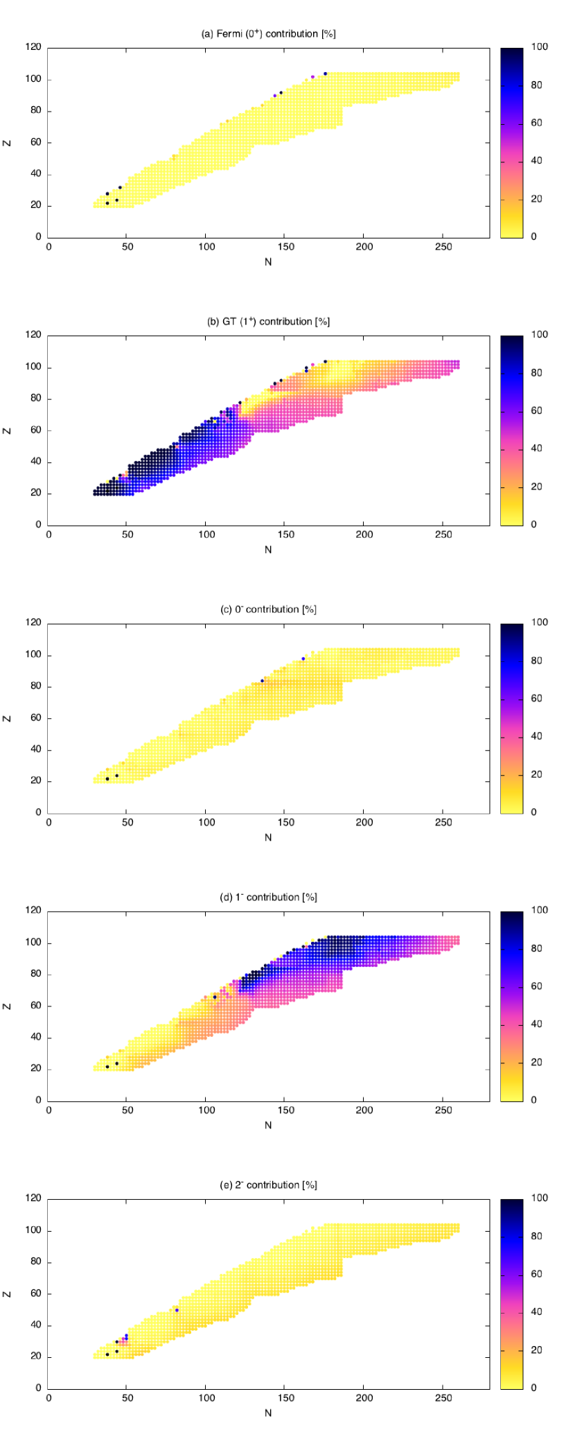
Fig. 4 also demonstrates the importance of going beyond the allowed approximation. In many heavy nuclei, the computed rates are dominated by the first-forbidden channel. Towards the drip line, both allowed and forbidden channels are important for all masses. The figure also shows that the non-unique $1^{-}$ channel is usually the most important of the forbidden multipoles. Thus any quenching of the (unique) $2^{-}$ channel and anti-quenching of the (non-unique) $0^{-}$ channel from meson-exchange currents Warburton (1991) would not have a significant impact on our overall results. In the $1^{-}$ channel the contributions of several different operators makes the effects of quenching hard to estimate.

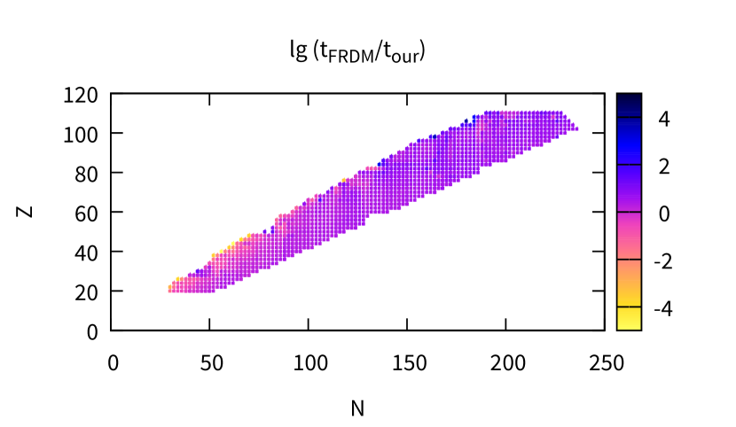
In Figure 5 we compare our half-lives to those of Möller et al. Möller et al. (2003) in all medium and heavy even-even isotopes. Our half-lives tend to be longer then those of Ref. Möller et al. (2003) close to the valley of stability in light nuclei and somewhat shorter in heavy nuclei (with significant forbidden contributions). Approaching the neutron drip line, the two computations yield similar results up to a constant offset in those of Ref. Möller et al. (2003) in even-even nuclei. All models can expect to do better near the drip line, where a significant fraction of the total $\beta$-decay strength can be below threshold.

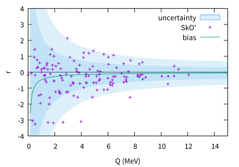
Because our naïve model for uncertainties is based on several assumptions that are only approximately correct or cannot easily be verified, we check its predictions where there are enough data to do so. Figure 6 shows the ratios of our half-lives to those of experiment together with the uncertainty model’s mean value and one- and two-standard-deviation bands, all as a function of ground-state $Q$ value. We can discount the model at very low $Q$ but it appears to work well above $Q\approx 4$ MeV. Out of the 72 nuclei, 48 (66.7%) fall within one standard deviation of the mean and 71 (98.6%) within two. These numbers are consistent with what one would expect from a normal distribution. The model quantifies our statement above that calculations are more accurate close to the drip line, where $Q$ is generally large.

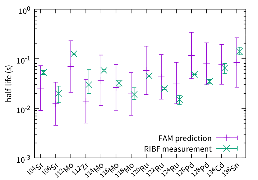
A recent RIBF measurement Lorusso et al. (2015) of 110 neutron-rich isotopes, 40 of them previously unknown, allows us to test the reliability of our predictions and especially our model for theoretical uncertainties. Because the data are so recent, we did not include them in any of our fits, and hence we are effectively using older data to predict the results of these new measurements. We have $28$ even-even nuclei with which to compare rates; for half of these there are earlier data in the ENSDF set (Figure 7). Our predictions agree with experiment to within our theoretical uncertainty (though our error bars may be a bit too large here). Our uncertainty model thus appears to be reasonable.

V Conclusions

Figure 5: Comparison of our computed half-lives in neutron-rich nuclei with those of Ref. Möller et al. (2003)

.

Figure 6: The fit 3A with the mean (green line) and one- and two-standard-deviation bands from our uncertainty model.

Figure 7: Our predictions for the $14$ half-lives of neutron-rich even-even nuclei measured only recently Lorusso et al. (2015) and not included in the ENSDF data set. All the measured half-lives fall within our one-sigma error bars, suggesting that our uncertainty estimates are too pessimistic in this particular region.

We have explored the ability of the axially-deformed Skyrme QRPA to provide a global description of beta-decay rates in even-even neutron-rich nuclei. With experimental rates and charge-exchange resonance energies as fitting targets we have found that among time-odd couplings, only those multiplying the isoscalar-pairing and the spin-density parts of the functional are well constrained; attempts to fit more than these two constants lead to overfitting. The tensor contributions to the energy-density functional are, in particular, not well constrained by this data. To get more accurate Skyrme-QRPA predictions, one can resort to local fits, i.e. $A$-dependent couplings. The recent work of Ref. Marketin et al. (2015), for example, attaches a sensible $A$ dependence to the strength of isoscalar pairing.

The level of agreement between our calculations and data throughout the isotopic chart is similar to that produced by other recent computations, in spite of our consistent inclusion of deformation, tensor terms in the functional, etc. It could be difficult to do much better without an account of multiphonon effects, as in the work, e.g., of Ref. Litvinova et al. (2014).

The most glaring shortcoming of our work here is the restriction to even-even nuclei. An extension of the FAM to odd-mass nuclei will be the subject of a future publication Shafer . For the moment, we make our results for the 1387 even-even neutron-rich nuclei, with crudely estimated theoretical uncertainties, available as supplementary material to this article.