Interior Point Method for Dynamic Constrained Optimization in Continuous Time

Mahyar Fazlyab, Santiago Paternain, Victor M. Preciado and Alejandro Ribeiro The authors are with the Department of Electrical and Systems Engineering, University of Pennsylvania, Philadelphia, PA 19104, USA. Email: {mahyarfa, spater, preciado, aribeiro}@seas.upenn.edu.
Abstract

This paper considers a class of convex optimization problems where both, the objective function and the constraints, have a continuously varying dependence on time. Our goal is to develop an algorithm to track the optimal solution as it continuously changes over time inside or on the boundary of the dynamic feasible set. We develop an interior point method that asymptotically succeeds in tracking this optimal point in nonstationary settings. The method utilizes a time varying constraint slack and a prediction-correction structure that relies on time derivatives of functions and constraints and Newton steps in the spatial domain. Error free tracking is guaranteed under customary assumptions on the optimization problems and time differentiability of objective and constraints. The effectiveness of the method is illustrated in a problem that involves multiple agents tracking multiple targets.

I Introduction

In a conventional optimization problem we are given a fixed objective and a fixed constraint and are tasked with finding the optimal argument that minimizes the objective among all feasible variables. In a time varying problem the objective and constraints change continuously in time and we are tasked with tracking the optimal point as it varies over time. These problems arise often in dynamical systems and control because many practical situations involve an objective function or a set of constraints that have dependence on time [1, 12, 5, 8]. Particular examples include estimation of the path of a stochastic process [9], signal detection with adaptive filters [4], tracking moving targets[20], and scheduling trajectories in an autonomous team of robots. [18]

Methods to solve convex optimization problems – say, gradient descent, Newton’s method, and interior point – are iterative in nature [3, 6]. When applied to a time varying nonstationary setting, each iteration moves the argument closer to the optimum while the optimum drifts away because of the changing nature of the objective and the constraints. This process is likely to settle into a steady state optimality gap that depends on the relative time constants of the dynamical process and the optimization algorithm. That this is indeed true has been observed and proven for gradient descent in unconstrained optimization [13], as well as in constrained optimization problems that arise in the specific contexts of distributed robotics [19], sequential estimation [9] and distributed optimization with a time varying alternating direction method of multipliers [10].

Alternatively, one can draw inspiration from the prediction-correction structure of Bayesian filters and utilize knowledge of the system’s dynamics to predict the drift of the optimal operating point and utilize the descent step of an optimization algorithm to correct the prediction. Variations of this idea have been developed in discrete [17] and continuous [2] time. When used in discrete time, the addition of a prediction step has been shown to reduce the tracking error relative to verbatim use of a descent algorithm [17, 16]. When used in continuous time, the use of a prediction step and a Newton correction results in perfect tracking of the optimal argument of an unconstrained optimization problem [2, 15].

This paper develops an interior point method to track the optimal point of a convex time varying constrained optimization problem (Section II). Important characteristics of this method are: (i) The use of a time time varying logarithmic barrier akin to the barrier used in static interior point methods. (ii) The use of a time varying constraint slack that is decreased over time and guarantees asymptotic satisfaction of the constraints. (iii) The use of time derivatives that play the role of a prediction step that tries to follow the movement of the optimal argument. (iv) The use of spatial Newton decrements that play the role of a correction step by pushing towards the current optimum. The main contribution of this paper is to show that this method converges to the time varying optimum under mild assumptions (Section III). These assumptions correspond to the customary requirements to prove convergence of interior point methods and differentiability of the objective and constraints with respect to time variations (Theorem 1). It is important to emphasize that our convergence result holds for nonstationary systems and, as such, do not rely on a vanishing rate of change. This implies that the proposed systems succeeds in tracking the optimum without error after a transient phase. The effectiveness of the method is illustrated in a problem that involves multiple agents tracking multiple targets (Section IV).

Notation and Preliminaries. Given an n-tuple (x1,,xn)subscript𝑥1subscript𝑥𝑛(x_{1},...,x_{n}), 𝐱n𝐱superscript𝑛\mathbf{x}\in\mathbb{R}^{n} is the associated vector. We denote as 𝐈nsubscript𝐈𝑛\mathbf{I}_{n} the n-dimensional identity matrix, as 𝕊nsuperscript𝕊𝑛\mathbb{S}^{n} the space of symmetric matrices and as 𝕊++nsubscriptsuperscript𝕊𝑛absent\mathbb{S}^{n}_{++} and 𝕊+nsubscriptsuperscript𝕊𝑛\mathbb{S}^{n}_{+} the spaces of positive definite and positive semidefinite matrices, respectively. For square matrices 𝐀𝐀\mathbf{A} and 𝐁𝐁\mathbf{B}, we write 𝐀𝐁succeeds-or-equals𝐀𝐁\mathbf{A}\succeq\mathbf{B} if and only if 𝐀𝐁𝐀𝐁\mathbf{A}-\mathbf{B} is positive semidefinite. The Euclidean norm of a vector 𝐱𝐱\mathbf{x} is 𝐱2subscriptnorm𝐱2\|\mathbf{x}\|_{2}. The gradient of the function f(x,t)𝑓x𝑡f(\textbf{x},t)\in\mathbb{R} with respect to xnxsuperscript𝑛\textbf{x}\in\mathbb{R}^{n} is denoted by xf(x,t)nsubscriptx𝑓x𝑡superscript𝑛\nabla_{\textbf{x}}f(\textbf{x},t)\in\mathbb{R}^{n}. The partial derivatives of xf(x,t)subscriptx𝑓x𝑡\nabla_{\textbf{x}}f(\textbf{x},t)with respect to x and t𝑡t are denoted by xxf(x,t)𝕊nsubscriptxx𝑓x𝑡superscript𝕊𝑛\nabla_{\textbf{x}\textbf{x}}f(\textbf{x},t)\in\mathbb{S}^{n} and xtf(x,t)nsubscriptx𝑡𝑓x𝑡superscript𝑛\nabla_{\textbf{x}t}f(\textbf{x},t)\in\mathbb{R}^{n}, respectively.

II Problem statement

Consider the following constrained convex optimization problem

x:=assignsuperscriptxabsent\displaystyle\textbf{x}^{\star}:= argminxnsubscriptxsuperscript𝑛\displaystyle\arg\min_{\textbf{x}\in\mathbb{R}^{n}} f0(x)subscript𝑓0x\displaystyle f_{0}(\textbf{x}) (1)
s.t. fi(x)0,i{1,,p}.formulae-sequencesubscript𝑓𝑖x0𝑖1𝑝\displaystyle f_{i}(\textbf{x})\leq 0,\quad i\in\{1,\cdots,p\}.

In order to solve (1), we can exploit interior point method [6, 14] in which we relax the constraints and penalize their violation by logarithmic functions of the form log(fi(x))subscript𝑓𝑖x-\log\left(-f_{i}(\textbf{x})\right). More specifically, we solve the relaxed problem

x(c):=argminx𝒟Φ(x,c),assignsuperscriptx𝑐subscriptx𝒟Φx𝑐\textbf{x}^{\star}(c):=\arg\min_{\textbf{x}\in\mathcal{D}}\,\Phi(\textbf{x},c), (2)

where the so-called barrier function Φ(x,c)Φx𝑐\Phi(\textbf{x},c) is defined as

Φ(x,c)=f0(x)1ci=1plog(fi(x)),Φx𝑐subscript𝑓0x1𝑐superscriptsubscript𝑖1𝑝subscript𝑓𝑖x\displaystyle\Phi(\textbf{x},c)=f_{0}(\textbf{x})-\frac{1}{c}\sum_{i=1}^{p}\log(-f_{i}(\textbf{x})), (3)

and 𝒟={xn|fi(x)<0,i=1,,p}𝒟conditional-setxsuperscript𝑛formulae-sequencesubscript𝑓𝑖x0𝑖1𝑝\mathcal{D}=\{\textbf{x}\in\mathbb{R}^{n}|f_{i}(\textbf{x})<0,i=1,\cdots,p\} is the interior of the feasible domain. Furthermore, c𝑐c is a positive constant such that x(c)xsuperscriptx𝑐superscriptx\textbf{x}^{\star}(c)\to\textbf{x}^{\star} as c𝑐c\to\infty.

To implement the interior point method, the unconstrained optimization problem (2) is solved sequentially for a positive growing sequence {ck}subscript𝑐𝑘\{c_{k}\}, each starting from the optimal solution of the previous optimization problem. The resulting sequence {x(ck)}superscriptxsubscript𝑐𝑘\{\textbf{x}^{\star}(c_{k})\} converges to the optimal point as cksubscript𝑐𝑘c_{k}\to\infty. For each fixed cksubscript𝑐𝑘c_{k}, x(ck)superscriptxsubscript𝑐𝑘\textbf{x}^{\star}(c_{k}) can be found, for instance, by Newton’s method as follows

ddtx(t)=xx1Φ(x(t),ck)xΦ(x(t),ck).𝑑𝑑𝑡x𝑡superscriptsubscriptxx1Φx𝑡subscript𝑐𝑘subscriptxΦx𝑡subscript𝑐𝑘\displaystyle\dfrac{d}{dt}\textbf{x}(t)=-\nabla_{\textbf{x}\textbf{x}}^{-1}\Phi(\textbf{x}(t),c_{k})\nabla_{\textbf{x}}\Phi(\textbf{x}(t),c_{k}). (4)

with initial condition x(0)=x(ck1)x0superscriptxsubscript𝑐𝑘1\textbf{x}(0)=\textbf{x}^{\star}(c_{k-1}). In order to decrease the total convergence time to the optimal point x(t)superscriptx𝑡\textbf{x}^{\star}(t), it is appealing to increase c𝑐c as a function of time, in lieu of discontinuous updates. Is this case, problem (3) would involve a time varying objective function.

In this paper, we consider a more general case in which both the objective function and/or the constraints are time-varying. More formally, we consider the following problem

x(t):=assignsuperscriptx𝑡absent\displaystyle\textbf{x}^{\star}(t):= argminxnsubscriptxsuperscript𝑛\displaystyle\arg\min_{\textbf{x}\in\mathbb{R}^{n}} f0(x,t)subscript𝑓0x𝑡\displaystyle f_{0}(\textbf{x},t) (5)
s.t. fi(x,t)0,i{1,,p}.formulae-sequencesubscript𝑓𝑖x𝑡0𝑖1𝑝\displaystyle f_{i}(\textbf{x},t)\leq 0,\quad i\in\{1,\cdots,p\}.

for all t[0,)𝑡0t\in[0,\infty). The ultimate goal is generate a (not necessarily feasible) solution x(t)x𝑡\textbf{x}(t) such that x(t)x(t)x𝑡superscriptx𝑡\textbf{x}(t)\to\textbf{x}^{\star}(t) as t𝑡t\to\infty, which necessarily enforces asymptotic feasibility. The corresponding time-varying barrier function of (5) becomes

Φ(x,t)=f0(x,t)1c(t)i=1plog(fi(x,t)),x𝒟(t)formulae-sequenceΦx𝑡subscript𝑓0x𝑡1𝑐𝑡superscriptsubscript𝑖1𝑝subscript𝑓𝑖x𝑡x𝒟𝑡\Phi(\textbf{x},t)=f_{0}(\textbf{x},t)-\frac{1}{c(t)}\sum_{i=1}^{p}\log\left(-f_{i}(\textbf{x},t)\right),\ \textbf{x}\in\mathcal{D}(t) (6)

where 𝒟(t):={xn|fi(x,t)<0,i=1,,p}assign𝒟𝑡conditional-setxsuperscript𝑛formulae-sequencesubscript𝑓𝑖x𝑡0𝑖1𝑝\mathcal{D}(t):=\{\textbf{x}\in\mathbb{R}^{n}|f_{i}(\textbf{x},t)<0,\ i=1,\cdots,p\} is the interior of the (time varying) feasible region, and c(t)𝑐𝑡c(t) is a positive valued function of time. For minimizing (6), we will propose a time-varying Newton differential equation whose solution x(t)x𝑡\textbf{x}(t) converges to x(t)superscriptx𝑡\textbf{x}^{\star}(t) as t𝑡t\to\infty.

For further analysis, we assume that the objective function is strongly convex in x and that the constraints are convex in x for all times t[0,)𝑡0t\in[0,\infty). In addition, we assume that fi(x,t)subscript𝑓𝑖x𝑡f_{i}(\textbf{x},t) is continuously differentiable with respect to time for all i{0,1,,p}𝑖01𝑝i\in\{0,1,\cdots,p\}. We formalize these assumptions next.

Assumption 1

The objective function f0(x,t)subscript𝑓0x𝑡f_{0}(\textbf{x},t) and the constraint functions fi(x,t)subscript𝑓𝑖x𝑡f_{i}(\textbf{x},t) are twice continuously differentiable with respect to x and continuously differentiable with respect to time for all t0𝑡0t\geq 0. Furthermore, f0(x,t)subscript𝑓0x𝑡f_{0}(\textbf{x},t) is uniformly strongly convex in x, i.e., xxf0(x,t)m𝐈succeeds-or-equalssubscriptxxsubscript𝑓0x𝑡𝑚𝐈\nabla_{\textbf{x}\textbf{x}}f_{0}(\textbf{x},t)\succeq m\mathbf{I} for some m>0𝑚0m>0 and f(x,t)𝑓x𝑡f(\textbf{x},t) is convex with respect to x for all t0𝑡0t\geq 0.

Assumption 2

Slater’s condition qualification holds for problem (5) for all t0𝑡0t\geq 0, i.e., there exits xnsuperscriptxsuperscript𝑛\textbf{x}^{\dagger}\in\mathbb{R}^{n} such that fi(x,t)<0subscript𝑓𝑖superscriptx𝑡0f_{i}(\textbf{x}^{\dagger},t)<0 for all t0𝑡0t\geq 0.

The above assumptions make the convexity-related properties to be invariant over time. With Assumption 2, the necessary and sufficient condition for optimality of problem (5) at all times t0𝑡0t\geq 0 read as

xf0(x(t),t)+i=1pλi(t)xfi(x(t),t)subscriptxsubscript𝑓0superscriptx𝑡𝑡superscriptsubscript𝑖1𝑝superscriptsubscript𝜆𝑖𝑡subscriptxsubscript𝑓𝑖superscriptx𝑡𝑡\displaystyle\nabla_{\textbf{x}}f_{0}(\textbf{x}^{\star}(t),t)+\sum_{i=1}^{p}\lambda_{i}^{\star}(t)\nabla_{\textbf{x}}f_{i}(\textbf{x}^{\star}(t),t) =0,absent0\displaystyle=0, (7)
λi(t)fi(x(t),t)superscriptsubscript𝜆𝑖𝑡subscript𝑓𝑖superscriptx𝑡𝑡\displaystyle\lambda_{i}^{\star}(t)f_{i}(\textbf{x}^{\star}(t),t) =0,i{1,,p}formulae-sequenceabsent0𝑖1𝑝\displaystyle=0,\ i\in\{1,\cdots,p\}
λi(t)superscriptsubscript𝜆𝑖𝑡\displaystyle\lambda_{i}^{\star}(t) 0,i{1,,p}formulae-sequenceabsent0𝑖1𝑝\displaystyle\geq 0,\ i\in\{1,\cdots,p\}
fi(x(t),t)subscript𝑓𝑖superscriptx𝑡𝑡\displaystyle f_{i}(\textbf{x}^{\star}(t),t) 0.absent0\displaystyle\leq 0.

where λ(t)=[λ1(t),,λp]Tpsuperscript𝜆𝑡superscriptsuperscriptsubscript𝜆1𝑡superscriptsubscript𝜆𝑝𝑇superscript𝑝\lambda^{\star}(t)=[\lambda_{1}^{\star}(t),\cdots,\lambda_{p}^{\star}]^{T}\in\mathbb{R}^{p} is the vector of optimal dual variables. Finally, we make a further assumption about the time variations of the optimal primal-dual pair.

Assumption 3

For any α>0𝛼0\alpha>0, the optimal dual variables satisfy λi(t)exp(αt)0superscriptsubscript𝜆𝑖𝑡𝛼𝑡0\lambda_{i}^{\star}(t)\exp(-\alpha t)\to 0 as t𝑡t\to\infty for all i{1,,p}𝑖1𝑝i\in\{1,\cdots,p\}.

The above assumption excludes the possibility for the optimal dual variables (and hence the optimal primal variables) to escape to infinity exponentially fast. Otherwise, the optimality conditions would become ill-conditioned as t𝑡t\to\infty and its solution is not tractable in the implementation phase. Equivalent assumtions to Assumption 3 are made in similar settings. See e.g. [17].

Prior to solving the general problem (5), we start off with unconstrained dynamic convex optimization where the optimization space is the domain of the objective function (Section III-A). In Section III-B we take time varying linear equality constraints into account and in Section III-C we deal with the case of generic dynamic convex constrained optimization problems. In section IV two tracking problems are studied that are posed as time varying optimization problems that can be solved through the techniques developed in Section III.

III Time-Varying Interior Point Method

In this section, we develop a time-varying interior point method that solves (5). We first introduce time-varying Newton method for unconstrained dynamic optimization problems. Next, we generalize the method to linear equality constraints. Finally, we incorporate time-varying interior point method for the case of inequality constraints.

III-A Unconstrained Time-Varying Convex optimization

In unconstrained time-varying convex optimization the goal is to track, continuously in time, the minimizer of a time-varying convex function. Mathematically speaking, given an objective function f0(x,t):n×+:subscript𝑓0x𝑡superscript𝑛subscriptf_{0}(\textbf{x},t):\mathbb{R}^{n}\times\mathbb{R}_{+}\to\mathbb{R}, the goal is estimate the trajectory x(t)superscriptx𝑡\textbf{x}^{\star}(t) where

x(t):=argminxnf0(x,t).assignsuperscriptx𝑡xsuperscript𝑛subscript𝑓0x𝑡\displaystyle\textbf{x}^{\star}(t):=\arg\underset{\textbf{x}\in\mathbb{R}^{n}}{\min}\quad f_{0}(\textbf{x},t). (8)

The optimal trajectory x(t)superscriptx𝑡\textbf{x}^{\star}(t) is characterized by the points where the gradient of f0(x,t)subscript𝑓0x𝑡f_{0}(\textbf{x},t) with respect to x is zero, i.e. xf0(x(t),t)0subscriptxsubscript𝑓0superscriptx𝑡𝑡0\nabla_{\textbf{x}}f_{0}(\textbf{x}^{\star}(t),t)\equiv 0 for all t[0,)𝑡0t\in[0,\infty). Using chain rule to differentiate the latter identity with respect to time yields

ddtxf0(x(t),t)=𝑑𝑑𝑡subscriptxsubscript𝑓0superscriptx𝑡𝑡absent\displaystyle\dfrac{d}{dt}\nabla_{\textbf{x}}f_{0}(\textbf{x}^{\star}(t),t)= xxf0(x(t),t)ddtx(t)+xtf0(x(t),t).subscriptxxsubscript𝑓0superscriptx𝑡𝑡𝑑𝑑𝑡superscriptx𝑡subscriptx𝑡subscript𝑓0superscriptx𝑡𝑡\displaystyle\nabla_{\textbf{x}\textbf{x}}f_{0}(\textbf{x}^{\star}(t),t)\dfrac{d}{dt}\textbf{x}^{\star}(t)+\nabla_{\textbf{x}t}f_{0}(\textbf{x}^{\star}(t),t). (9)

The left hand side of the above equation is identically zero for t[0,)𝑡0t\in[0,\infty). It follows that the optimal solution moves with a velocity given by

ddtx(t)=xx1f0(x(t),t)xtf0(x(t),t).𝑑𝑑𝑡superscriptx𝑡superscriptsubscriptxx1subscript𝑓0superscriptx𝑡𝑡subscriptx𝑡subscript𝑓0superscriptx𝑡𝑡\displaystyle\dfrac{d}{dt}\textbf{x}^{\star}(t)=-\nabla_{\textbf{x}\textbf{x}}^{-1}f_{0}(\textbf{x}^{\star}(t),t)\nabla_{\textbf{x}t}f_{0}(\textbf{x}^{\star}(t),t). (10)

The above observation suggests that the tracking trajectory should evolve with (approximately) the same velocity as the minimizer trajectory, while taking a descent direction at the same time in order to get closer to the optimal trajectory. If Newton-method is chosen as the descent direction, the resulting time-varying Newton method takes the form

x˙(t)=xx1f0(x(t),t)[𝐏xf0(x(t),t)+xtf0(x(t),t)],˙x𝑡superscriptsubscriptxx1subscript𝑓0x𝑡𝑡delimited-[]𝐏subscriptxsubscript𝑓0x𝑡𝑡subscriptx𝑡subscript𝑓0x𝑡𝑡\displaystyle\dot{\textbf{x}}(t)=-{\nabla_{\textbf{x}\textbf{x}}^{-1}f_{0}(\textbf{x}(t),t)}[\mathbf{P}\nabla_{\textbf{x}}f_{0}(\textbf{x}(t),t)+\nabla_{\textbf{x}t}f_{0}(\textbf{x}(t),t)], (11)

where 𝐏𝐏\mathbf{P} is a positive definite matrix. The next lemma shows that the solution of the dynamical system (11) converges exponentially to the solution to the unconstrained minimization problem (8).

Lemma 1

Let x(t)superscriptx𝑡\textbf{x}^{\star}(t) be defined as in (8) and x(t)x𝑡\textbf{x}(t) be the solution of the differential equation (11) with 𝐏𝕊++n𝐏subscriptsuperscript𝕊𝑛absent\mathbf{P}\in\mathbb{S}^{n}_{++} satisfying 𝐏σ𝐈succeeds-or-equals𝐏𝜎𝐈\mathbf{P}\succeq\sigma{\mathbf{I}}. Then, the following inequality holds

x(t)x(t)2C(x0,m)eσt,subscriptnormx𝑡superscriptx𝑡2𝐶subscriptx0𝑚superscript𝑒𝜎𝑡\|\textbf{x}(t)-\textbf{x}^{\star}(t)\|_{2}\leq C(\textbf{x}_{0},m)e^{-\sigma t},

where x0subscriptx0\textbf{x}_{0} is an arbitrary initial point and 0C(x0,m)<0𝐶subscriptx0𝑚0\leq C(\textbf{x}_{0},m)<\infty.

Proof.

The proof is found in Appendix subsection A-A. ∎

The previous lemma confirms that the trajectory generated by (11) converges exponentially to the optimal trajectory and therefore it is possible to solve the unconstrained time-varying optimization problem (8) by discretization of the dynamical system (11). Next, we show that the same dynamical system allows us to solve dynamic optimization problems with equality constraints by augmenting the state space with the Lagrange multipliers associated with the equality constraints.

III-B Equality-Constraint Time-Varying Convex Optimization

Consider the problem of tracking the minimizer of a convex time-varying objective function subject to linear constraints. More precisely, we seek to estimate x(t)superscriptx𝑡\textbf{x}^{\star}(t) for all t[0,)𝑡0t\in[0,\infty) where

x(t):=assignsuperscriptx𝑡absent\displaystyle\textbf{x}^{\star}(t):= argminxnxsuperscript𝑛\displaystyle\arg\underset{\textbf{x}\in\mathbb{R}^{n}}{\min} f0(x,t)subscript𝑓0x𝑡\displaystyle f_{0}(\textbf{x},t) (12)
s.t. 𝐀(t)x=b(t),𝐀𝑡xb𝑡\displaystyle\mathbf{A}(t)\textbf{x}=\textbf{b}(t),

with 𝐀(t)p×n𝐀𝑡superscript𝑝𝑛\mathbf{A}(t)\in\mathbb{R}^{p\times n} and rank(𝐀(t))=p<nrank𝐀𝑡𝑝𝑛\mbox{rank}(\mathbf{A}(t))=p<n for all t0𝑡0t\geq 0. The Lagrangian relaxation of (12) is

(x,λ,t)=f0(x,t)+λT(𝐀(t)xb(t)).x𝜆𝑡subscript𝑓0x𝑡superscript𝜆𝑇𝐀𝑡xb𝑡\displaystyle\mathcal{L}(\textbf{x},\lambda,t)=f_{0}(\textbf{x},t)+\lambda^{T}(\mathbf{A}(t)\textbf{x}-\textbf{b}(t)). (13)

where λp𝜆superscript𝑝\lambda\in\mathbb{R}^{p} is the vector of Lagrange multipliers. The optimal trajectory (x(t),λ(t))superscriptx𝑡superscript𝜆𝑡(\textbf{x}^{\star}(t),\lambda^{\star}(t)) constitutes of points where the gradient of the Lagrangian with respect to both x and λ𝜆\lambda vanishes. Therefore, by extending the state space to be z:=[xTλT]Tn+passignzsuperscriptdelimited-[]superscriptx𝑇superscript𝜆𝑇𝑇superscript𝑛𝑝\textbf{z}:=[\textbf{x}^{T}\ \lambda^{T}]^{T}\in\mathbb{R}^{n+p}, the optimal solution z(t)superscriptz𝑡\textbf{z}^{\star}(t) is characterized by

z(z(t),t)=0,t0.formulae-sequencesubscriptzsuperscriptz𝑡𝑡0𝑡0\nabla_{\textbf{z}}\mathcal{L}(\textbf{z}^{\star}(t),t)=0,\ t\geq 0. (14)

Similar to the unconstrained case, the tracking trajectory should compose of two directions: a velocity compensating direction and a descent direction. The next lemma addresses the algorithm for tracking x(t)superscriptx𝑡\textbf{x}^{\star}(t) in (12).

Lemma 2

Denote z(t)=[x(t)Tλ(t)T]Tz𝑡superscriptdelimited-[]xsuperscript𝑡𝑇𝜆superscript𝑡𝑇𝑇\textbf{z}(t)=[\textbf{x}(t)^{T}\ \lambda(t)^{T}]^{T} as the solution of the following differential equation

ddtz(t)=zz1(z(t),t)(𝐏z(z(t),t)+zt(z(t),t))𝑑𝑑𝑡z𝑡superscriptsubscriptzz1z𝑡𝑡𝐏subscriptzz𝑡𝑡subscriptz𝑡z𝑡𝑡\displaystyle\dfrac{d}{dt}\textbf{z}(t)=-\nabla_{\textbf{z}\textbf{z}}^{-1}\mathcal{L}(\textbf{z}(t),t)(\mathbf{P}\nabla_{\textbf{z}}\mathcal{L}(\textbf{z}(t),t)+\nabla_{\textbf{z}t}\mathcal{L}(\textbf{z}(t),t)) (15)

where \mathcal{L} is defined in (13) and 𝐏𝕊n+p𝐏superscript𝕊𝑛𝑝\mathbf{P}\in\mathbb{S}^{n+p} is a positive definite matrix satisfying 𝐏σ𝐈n+psucceeds-or-equals𝐏𝜎subscript𝐈𝑛𝑝\mathbf{P}\succeq\sigma\mathbf{I}_{n+p}. Then, the following inequality holds

x(t)x(t)22+λ(t)λ(t)22C(x0,λ0,m)e2σt.superscriptsubscriptnormx𝑡superscriptx𝑡22superscriptsubscriptnorm𝜆𝑡superscript𝜆𝑡22𝐶subscriptx0subscript𝜆0𝑚superscript𝑒2𝜎𝑡\displaystyle\|\textbf{x}(t)-\textbf{x}^{\star}(t)\|_{2}^{2}+\|\lambda(t)-\lambda^{\star}(t)\|_{2}^{2}\leq C(\textbf{x}_{0},\lambda_{0},m)e^{-2\sigma t}. (16)

where x0nsubscriptx0superscript𝑛\textbf{x}_{0}\in\mathbb{R}^{n} and λ0psubscript𝜆0superscript𝑝\lambda_{0}\in\mathbb{R}^{p} are arbitrary initial points and 0C(x0,λ0,m)<0𝐶subscriptx0subscript𝜆0𝑚0\leq C(\textbf{x}_{0},\lambda_{0},m)<\infty.

Proof.

See Appendix subsection A-B. ∎

Notice that the dynamical system (15) needs not to start from a feasible point, i.e. it is not required that 𝐀0x0=𝐛0subscript𝐀0subscriptx0subscript𝐛0\mathbf{A}_{0}\textbf{x}_{0}=\mathbf{b}_{0}. However, feasibility is achieved exponentially fast by (16).

In the sequel, we consider the most general case with time-varying inequality constraints. Without loss of generally, we omit linear equality constraints as each single affine equality constraint can be expressed as two convex inequality constraints.

III-C Time-Varying Interior-point method

In this section, we return to the general optimization problem (5) with the associated barrier function (6). We will show that the same differential equation developed in Section III-A – using the barrier function Φ(x,t)Φx𝑡\Phi(\textbf{x},t) defined in (6) in lieu of f0(x,t)subscript𝑓0x𝑡f_{0}(\textbf{x},t) in (11) – pushes the generated solution to the optimal trajectory when the barrier parameter c(t)𝑐𝑡c(t)\to\infty. Formally, the dynamical system of interest is

x˙(t)=xx1Φ(x(t),t)(𝐏xΦ(x(t),t)+xtΦ(x(t),t)),˙x𝑡superscriptsubscriptxx1Φx𝑡𝑡𝐏subscriptxΦx𝑡𝑡subscriptx𝑡Φx𝑡𝑡\displaystyle\dot{\textbf{x}}(t)=-\nabla_{\textbf{x}\textbf{x}}^{-1}\Phi(\textbf{x}(t),t)\left(\mathbf{P}\nabla_{\textbf{x}}\Phi(\textbf{x}(t),t)+\nabla_{\textbf{x}t}\Phi(\textbf{x}(t),t)\right), (17)

where 𝐏𝕊++n𝐏subscriptsuperscript𝕊𝑛absent\mathbf{P}\in\mathbb{S}^{n}_{++}. Notice, however, that the Newton method in this case needs to start from a strictly feasible point, i.e. x0𝒟0subscriptx0subscript𝒟0\textbf{x}_{0}\in\mathcal{D}_{0}. This limitation is not desirable, as it is not always straightforward to find such an initial condition. This restriction can be overcome by expanding the feasible region at t=0𝑡0t=0 by a slack variable, denoted by s𝑠s, and shrink it to the real feasible set over time. More precisely, we perturb problem (5) at each time t[0,)𝑡0t\in[0,\infty) by s(t):+++:𝑠𝑡subscriptsubscriptabsents(t):\mathbb{R}_{+}\to\mathbb{R}_{++} as follows

x~(t):=assignsuperscript~x𝑡absent\displaystyle\tilde{\textbf{x}}^{\star}(t):= argminxnsubscriptxsuperscript𝑛\displaystyle\arg\min_{\textbf{x}\in\mathbb{R}^{n}} f0(x,t)subscript𝑓0x𝑡\displaystyle f_{0}(\textbf{x},t) (18)
s.t. fi(x,t)s(t),i{1,,p}.formulae-sequencesubscript𝑓𝑖x𝑡𝑠𝑡𝑖1𝑝\displaystyle f_{i}(\textbf{x},t)\leq s(t),\quad i\in\{1,\cdots,p\}.

It can be observed that the feasible region is enlarged for s(t)0𝑠𝑡0s(t)\geq 0. In particular, at time t=0𝑡0t=0, any initial point x0nsubscriptx0superscript𝑛\textbf{x}_{0}\in\mathbb{R}^{n} can be made feasible by choosing the initial s0=s(0)subscript𝑠0𝑠0s_{0}=s(0) large enough. Another consequence of such perturbation is that, the optimal value of the perturbed problem (18) is no larger than the optimal value at x(t)superscriptx𝑡\textbf{x}^{\star}(t). The next lemma formalizes this observation.

Lemma 3

Let x(t)superscriptx𝑡\textbf{x}^{\star}(t) be defined as in (5) and x~(t)superscript~x𝑡\tilde{\textbf{x}}^{\star}(t) as in (18). Then, the following inequality holds:

0f0(x(t),t)f0(x~(t),t)i=1pλi(t)s(t)0subscript𝑓0superscriptx𝑡𝑡subscript𝑓0superscript~x𝑡𝑡superscriptsubscript𝑖1𝑝subscriptsuperscript𝜆𝑖𝑡𝑠𝑡\displaystyle 0\leq f_{0}(\textbf{x}^{\star}(t),t)-f_{0}(\tilde{\textbf{x}}^{\star}(t),t)\leq\sum_{i=1}^{p}\lambda^{\star}_{i}(t)s(t) (19)

where λi(t),i{1,,p}superscriptsubscript𝜆𝑖𝑡𝑖1𝑝\lambda_{i}^{\star}(t),\ i\in\{1,\cdots,p\} are optimal dual variables defined in (7).

Proof.

See Appendix subsection A-C. ∎

The above lemma asserts that the sub-optimality of the perturbed solution x~(t)superscript~x𝑡\tilde{\textbf{x}}^{\star}(t) is controlled by s(t)𝑠𝑡s(t). More importantly, as a result of Assumption 3, the sub-optimality can be pushed to zero if s(t)=s0exp(αt)𝑠𝑡subscript𝑠0𝛼𝑡s(t)=s_{0}\exp(-\alpha t) for any α>0𝛼0\alpha>0.

The barrier function associated with the problem (18) is

Φ~(x,t)=f0(x,t)1c(t)i=1plog(s(t)fi(x,t)),x𝒟~(t)formulae-sequence~Φx𝑡subscript𝑓0x𝑡1𝑐𝑡superscriptsubscript𝑖1𝑝𝑠𝑡subscript𝑓𝑖x𝑡x~𝒟𝑡\displaystyle\tilde{\Phi}(\textbf{x},t)=f_{0}(\textbf{x},t)-\frac{1}{c(t)}\sum_{i=1}^{p}\log\left(s(t)-f_{i}(\textbf{x},t)\right),\ \textbf{x}\in\mathcal{\tilde{D}}(t) (20)

where 𝒟~(t):={xn|fi(x,t)<s(t),i=1,,p}assign~𝒟𝑡conditional-set𝑥superscript𝑛formulae-sequencesubscript𝑓𝑖x𝑡𝑠𝑡𝑖1𝑝\tilde{\mathcal{D}}(t):=\{x\in\mathbb{R}^{n}\ |f_{i}(\textbf{x},t)<s(t),\ i=1,\cdots,p\} is the perturbed domain. For any initial point x0nsubscriptx0superscript𝑛\textbf{x}_{0}\in\mathbb{R}^{n}, s0subscript𝑠0s_{0} can be chosen large enough such that x0𝒟~0subscript𝑥0subscript~𝒟0x_{0}\in\mathcal{\tilde{D}}_{0}. More precisely, we must have that

s0={0ifmaxifi(x0,0)0maxifi(x0,0)+εifmaxifi(x0,0)>0subscript𝑠0cases0ifsubscript𝑖subscript𝑓𝑖subscriptx000subscript𝑖subscript𝑓𝑖subscriptx00𝜀ifsubscript𝑖subscript𝑓𝑖subscriptx000\displaystyle s_{0}=\begin{cases}0&\mbox{if}\ \max_{i}\ f_{i}(\textbf{x}_{0},0)\leq 0\\ \max_{i}f_{i}(\textbf{x}_{0},0)+\varepsilon&\mbox{if}\ \max_{i}\ f_{i}(\textbf{x}_{0},0)>0\end{cases} (21)

for some ε>0𝜀0\varepsilon>0. Denote by z~(t)superscript~z𝑡\tilde{\textbf{z}}^{\star}(t) as the minimizer of the perturbed barrier function (20), i.e.

z~(t):=assignsuperscript~z𝑡absent\displaystyle\tilde{\textbf{z}}^{\star}(t):= argminx𝒟~(t)Φ~(x,t)x~𝒟𝑡~Φx𝑡\displaystyle\arg\underset{\textbf{x}\in\mathcal{\tilde{D}}(t)}{\min}\tilde{\Phi}(\textbf{x},t) (22)

For solving (22), we can now apply time-varying Newton method to get the following differential equation

z~˙(t)=xx1Φ~(z~(t),t)(𝐏xΦ~(z~(t),t)+xtΦ~(z~(t),t)),˙~z𝑡superscriptsubscriptxx1~Φ~z𝑡𝑡𝐏subscriptx~Φ~z𝑡𝑡subscriptx𝑡~Φ~z𝑡𝑡\displaystyle\dot{\tilde{\textbf{z}}}(t)=-\nabla_{{\textbf{x}}{\textbf{x}}}^{-1}\tilde{\Phi}(\tilde{\textbf{z}}(t),t)\left(\mathbf{P}\nabla_{{\textbf{x}}}\tilde{\Phi}(\tilde{\textbf{z}}(t),t)+\nabla_{{\textbf{x}}t}\tilde{\Phi}(\tilde{\textbf{z}}(t),t)\right), (23)

By increasing the barrier parameter c(t)𝑐𝑡c(t) over time the sub-optimality is decreased as we show in the next lemma.

Lemma 4

With z~(t)superscript~z𝑡\tilde{\textbf{z}}^{\star}(t) defined as in (22) and x~(t)superscript~x𝑡\tilde{\textbf{x}}^{\star}(t) as in (18), the following inequality holds for all t0𝑡0t\geq 0

0f0(z~(t),t)f0(x~(t),t)pc(t)0subscript𝑓0superscript~z𝑡𝑡subscript𝑓0superscript~x𝑡𝑡𝑝𝑐𝑡\displaystyle 0\leq f_{0}(\tilde{\textbf{z}}^{\star}(t),t)-f_{0}(\tilde{\textbf{x}}^{\star}(t),t)\leq\dfrac{p}{c(t)} (24)
Proof.

The proof is provided in Appendix subsection A-D. ∎

The bound (24) quantifies the sub-optimality of z~(t)superscript~z𝑡\tilde{\textbf{z}}^{\star}(t) with respect to the perturbed optimal trajectory x~(t)superscript~x𝑡\tilde{\textbf{x}}^{\star}(t). More specifically, as c(t)𝑐𝑡c(t)\to\infty, z~(t)x~(t)superscript~z𝑡superscript~x𝑡\tilde{\textbf{z}}^{\star}(t)\to\tilde{\textbf{x}}^{\star}(t). The next lemma established this convergence under the dynamics (23).

Lemma 5

Consider problem (18) with the corresponding time-varying barrier function (20). Let z~(t)~z𝑡\tilde{\textbf{z}}(t) be the solution of the differential equation (23) with 𝐏𝕊++n𝐏subscriptsuperscript𝕊𝑛absent\mathbf{P}\in\mathbb{S}^{n}_{++} satisfying 𝐏σ𝐈succeeds-or-equals𝐏𝜎𝐈\mathbf{P}\succeq\sigma{\mathbf{I}}, and initial condition x0nsubscriptx0superscript𝑛\textbf{x}_{0}\in\mathbb{R}^{n}. Finally, let s0subscript𝑠0s_{0} be chosen as in (21). Then, the following inequality holds

z~(t)z~(t)2C(x0,c0,s0,m)eσtsubscriptnorm~z𝑡superscript~z𝑡2𝐶subscriptx0subscript𝑐0subscript𝑠0𝑚superscript𝑒𝜎𝑡\displaystyle\|\tilde{\textbf{z}}(t)-\tilde{\textbf{z}}^{\star}(t)\|_{2}\leq C(\textbf{x}_{0},c_{0},s_{0},m)e^{-\sigma t} (25)

where 0C(x0,c0,s0,m)<0𝐶subscriptx0subscript𝑐0subscript𝑠0𝑚0\leq C(\textbf{x}_{0},c_{0},s_{0},m)<\infty.

Proof.

The proof is provided in Appendix subsection A-E. ∎

Few comments are in order: First, Lemma 5 shows that the solution z~(t)~z𝑡\tilde{\textbf{z}}(t) of the dynamical system (23) converges exponentially to the sub-optimal solution z~(t)superscript~z𝑡\tilde{\textbf{z}}^{\star}(t) in (22). Second, Lemma 4 guarantees that z~(t)superscript~z𝑡\tilde{\textbf{z}}^{\star}(t) converges to the optimal perturbed solution x~(t)superscript~x𝑡\tilde{\textbf{x}}^{\star}(t) in (18) if c(t)𝑐𝑡c(t)\to\infty. Finally, Lemma 3 confirms that the perturbed solution x~(t)superscript~x𝑡\tilde{\textbf{x}}^{\star}(t) converges to x(t)superscriptx𝑡\textbf{x}^{\star}(t) of the original problem (5) if s(t)0𝑠𝑡0s(t)\to 0. Therefore, convergence of the dynamical system (23) to the desired optimal solution x(t)superscriptx𝑡\textbf{x}^{\star}(t) is guaranteed if limtc(t)=subscript𝑡𝑐𝑡\lim_{t\to\infty}c(t)=\infty and s(t)0𝑠𝑡0s(t)\to 0 as t𝑡t\to\infty. The next theorem summarizes these observations as the main result of this section.

Theorem 1

Consider problem (5) with optimal trajectory x(t)superscriptx𝑡\textbf{x}^{\star}(t) and the corresponding barrier function (20). Let z~(t)~z𝑡\tilde{\textbf{z}}(t) be the solution of (23) with arbitrary initial condition x0nsubscriptx0superscript𝑛\textbf{x}_{0}\in\mathbb{R}^{n}. Finally, let c(t)𝑐𝑡c(t)\to\infty and s(t)=s0exp(αt)𝑠𝑡subscript𝑠0𝛼𝑡s(t)=s_{0}\exp(-\alpha t) for some α>0𝛼0\alpha>0 and s0subscript𝑠0s_{0} chosen according to (21). Then, z~(t)x(t)~z𝑡superscriptx𝑡\tilde{\textbf{z}}(t)\to\textbf{x}^{\star}(t) as t𝑡t\to\infty.

Proof.

The proof follows from inequalities (19), (24) and (25). ∎

We close this section by two remarks.

Remark 1

The logarithmic barrier coefficient c(t)𝑐𝑡c(t) is required to be positive, monotonic increasing, asymptotically converging to infinity, and be bounded in finite time. A convenient choice could be c(t)=c0exp(αt)𝑐𝑡subscript𝑐0𝛼𝑡{c}(t)=c_{0}\exp(\alpha t) for α>0𝛼0\alpha>0. Notice that the term xtΦ(z~(t),t)subscriptx𝑡Φ~z𝑡𝑡\nabla_{\textbf{x}t}\Phi(\tilde{\textbf{z}}(t),t) in (23) compensates for continuous-time variation of both c(t)𝑐𝑡c(t) and s(t)𝑠𝑡s(t).

Remark 2

If the Newton differential equation (23) starts from a strictly feasible initial point, i.e. x0𝒟0subscriptx0subscript𝒟0\textbf{x}_{0}\in\mathcal{D}_{0}, then s(t)𝑠𝑡s(t) is chosen to be identically zero. From inequality (19), x~(t)=x(t)~x𝑡x𝑡\tilde{\textbf{x}}(t)=\textbf{x}(t) for t0𝑡0t\geq 0. Therefore, according to inequalities (24) and (25), exponential convergence of the tracking trajectory z~(t)~z𝑡\tilde{\textbf{z}}(t) to the optimal trajectory x(t)superscriptx𝑡\textbf{x}^{\star}(t) is guaranteed if the barrier parameter c(t)𝑐𝑡c(t) grows exponentially.

IV Numerical experiments
Refer to caption
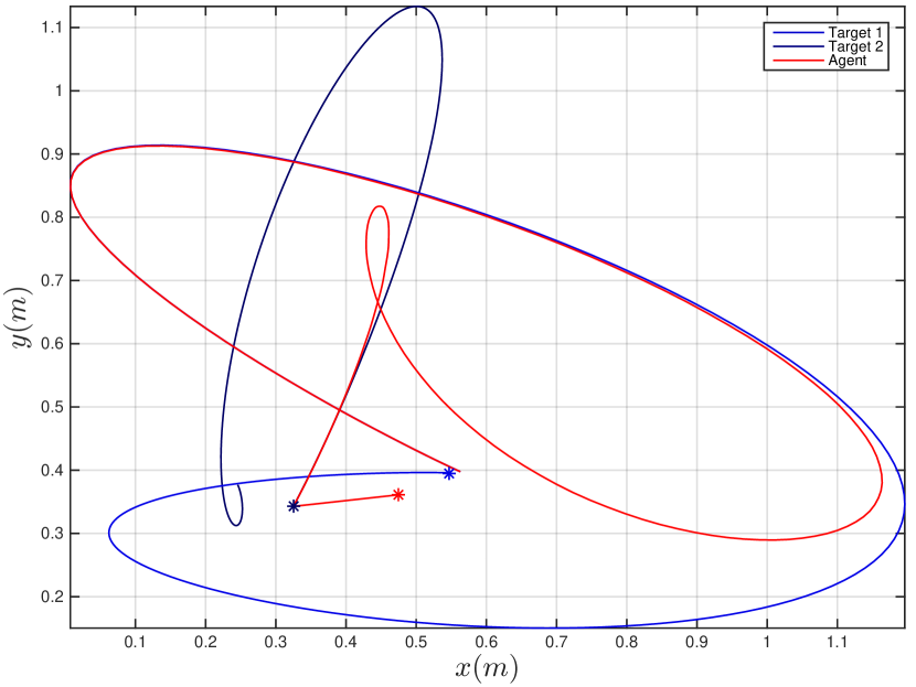
Figure 1: Trajectory of the agent –in red– and the targets. The agent starts off with the first target and then switches to the second one. The gain matrix is set to be 𝐏=10I2𝐏10subscript𝐼2\mathbf{P}=10I_{2}.
Refer to caption
Figure 2: Tracking error x(t)x(t)normx𝑡superscriptx𝑡\|\textbf{x}(t)-\textbf{x}^{*}(t)\| as a function of time for the unconstrained problem. The optimal solution x(t)superscriptx𝑡\textbf{x}^{\star}(t) has been computed in discrete times of Euler integration using CVX [7].

In this section, we evaluate the performance of the time varying interior point method developed in the previous section by two numerical examples. In Section IV-A we numerically solve an unconstrained dynamic convex problem and in Section IV-B we study a constrained dynamic convex problem. In implementations, we use Euler integration scheme with variable step size to solve the differential equations that generate the solution.

IV-A Unconstrained optimization

Consider an agent charged with the task of tracking two targets sequentially. That is, the agent is required to track the first target on the time interval [t0,tint]subscript𝑡0subscript𝑡𝑖𝑛𝑡[t_{0},t_{int}] and track the other target on the time interval [tint,tf]subscript𝑡𝑖𝑛𝑡subscript𝑡𝑓[t_{int},t_{f}]. If we denote the position of the i𝑖ith target by yi(t)subscripty𝑖𝑡\textbf{y}_{i}(t), the objective function takes the form

f0(x,t)=S(t)xy1(t)2+(1S(t))xy2(t)2,subscript𝑓0x𝑡𝑆𝑡superscriptnormxsubscripty1𝑡21𝑆𝑡superscriptnormxsubscripty2𝑡2f_{0}(\textbf{x},t)=S(t)\|\textbf{x}-\textbf{y}_{1}(t)\|^{2}+(1-S(t))\|\textbf{x}-\textbf{y}_{2}(t)\|^{2}, (26)

where S(t)𝑆𝑡S(t) is a weighting function that determines which target must be tracked. We consider the following differentiable switch

S(t)=111+eγ(ttint),𝑆𝑡111superscript𝑒𝛾𝑡subscript𝑡𝑖𝑛𝑡S(t)=1-\frac{1}{1+e^{-\gamma(t-t_{int})}}, (27)

where γ>0𝛾0\gamma>0 controls the speed with which S(t)𝑆𝑡S(t) transitions from one to zero.

We use a time parametric representation of the trajectories of the targets. Specifically, let pj(t)subscript𝑝𝑗𝑡p_{j}(t) be elements of a polynomial basis, the k𝑘kth component of the trajectory of target i𝑖ith is given by

yik(t)=j=0ni1yikjpj(t),subscript𝑦𝑖𝑘𝑡superscriptsubscript𝑗0subscript𝑛𝑖1subscript𝑦𝑖𝑘𝑗subscript𝑝𝑗𝑡y_{ik}(t)=\sum_{j=0}^{n_{i}-1}y_{ikj}p_{j}(t), (28)

where nisubscript𝑛𝑖n_{i} is the total number of polynomials that parametrize the path traversed by target i𝑖i and yik,jsubscript𝑦𝑖𝑘𝑗y_{ik,j} represent the corresponding nisubscript𝑛𝑖n_{i} coefficients. To determine the coefficients yik,jsubscript𝑦𝑖𝑘𝑗y_{ik,j} we draw at random a total of L𝐿L random points per target {y~i}=1Lsuperscriptsubscriptsuperscriptsubscript~𝑦𝑖1𝐿\{\tilde{y}_{\ell}^{i}\}_{\ell=1}^{L} independently and uniformly in the unit box [0,1]2superscript012[0,1]^{2}. Target i𝑖i is required to pass trough the points y~isuperscriptsubscript~𝑦𝑖\tilde{y}_{\ell}^{i} at times tf/(L+1)subscript𝑡𝑓𝐿1\ell t_{f}/(L+1). Paths yi(t)subscript𝑦𝑖𝑡y_{i}(t) are then chosen such that the path integral of the acceleration squared is minimized subject to the constraints of each individual path, i.e;

yi=subscript𝑦𝑖absent\displaystyle y_{i}= argmin\displaystyle\arg\min 0Ty¨i(t)2𝑑t,superscriptsubscript0𝑇superscriptnormsubscript¨𝑦𝑖𝑡2differential-d𝑡\displaystyle\int_{0}^{T}\|\ddot{y}_{i}(t)\|^{2}dt,
s.tformulae-sequence𝑠𝑡\displaystyle s.t yi(tf/(L+1))=y~ifor all=0,1L+1.formulae-sequencesubscript𝑦𝑖subscript𝑡𝑓𝐿1superscriptsubscript~𝑦𝑖for all01𝐿1\displaystyle y_{i}(\ell t_{f}/(L+1))=\tilde{y}_{\ell}^{i}\quad\mbox{for all}\quad\ell=0,1\ldots L+1. (29)

This problem can be solved by a quadratic program [11]. In subsequent numerical experiment, we set the number of targets to m=2𝑚2m=2, the time interval to [0,1]01[0,1], and the intermediate switching time tint=1/2subscript𝑡𝑖𝑛𝑡12t_{int}=1/2. We use the standard polynomial basis pj(t)=tjsubscript𝑝𝑗𝑡superscript𝑡𝑗p_{j}(t)=t^{j} in (28) and the degree of the polynomials is set to be n=30𝑛30n=30 for i=1,,m𝑖1𝑚i=1,\cdots,m. To generate the target paths, we consider a total of L=5𝐿5L=5 random chosen intermediate points. We further set the parameter controlling the switching speed to γ=20𝛾20\gamma=20. For this data, we solve (11) by Euler integration with variable step size of maximum length 0.01s0.01𝑠0.01s.

The resulting trajectories are illustrated in Figure 1 when we select the gain matrix in (11) to be 𝐏=10𝐈2𝐏10subscript𝐈2\mathbf{P}=10\mathbf{I}_{2}. A qualitative examination of this behavior shows that the agent –in red – succeeds in tracking the first target up to time t=0.5s𝑡0.5𝑠t=0.5s and switching to the second agent after t=0.5s𝑡0.5𝑠t=0.5s. The objective function considered in (26) agrees with Assumption 1 and therefore, the hypothesis of Lemma 1 is satisfied. Consequently, exponential convergence to the optimal solution is guaranteed as it can be observed in Figure 2. Also, this convergence gets faster as the gain matrix 𝐏𝐏\mathbf{P} is increased.

IV-B Constrained optimization
Refer to caption
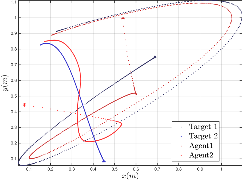
Figure 3: Trajectory of the agent –in red– and the targets to track. It can be observed that the agents succeed in following both targets while keeping the distance between them as small as possible. The gain matrix is set to be 𝐏=50𝐈2𝐏50subscript𝐈2\mathbf{P}=50\mathbf{I}_{2}.
Refer to caption
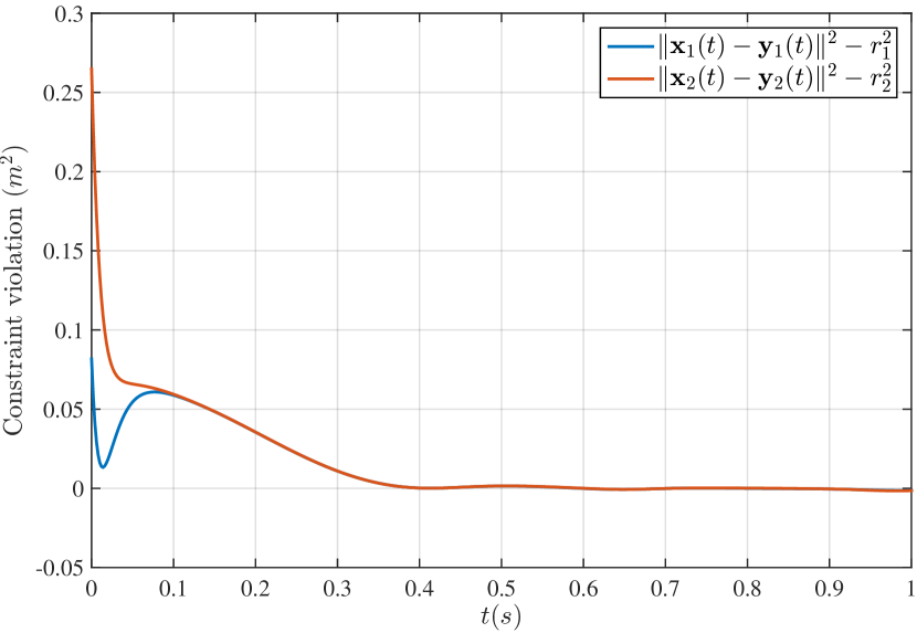
(a) Time evolution of constraint functions xi(t)yi(t)2ri2subscriptnormsubscriptx𝑖𝑡subscripty𝑖𝑡2superscriptsubscript𝑟𝑖2\|\textbf{x}_{i}(t)-\textbf{y}_{i}(t)\|_{2}-r_{i}^{2} for i=1,2𝑖12i=1,2.
Refer to caption
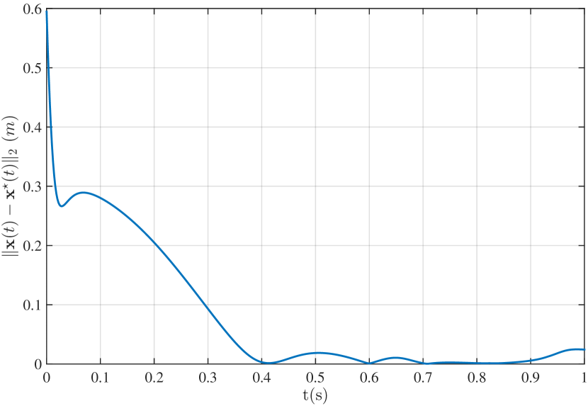
(b) Time evolution of [x1(t)x1(x),x2(t)x2(t)]2subscriptnormsubscriptx1𝑡superscriptsubscriptx1𝑥subscriptx2𝑡superscriptsubscriptx2𝑡2\left\|[\textbf{x}_{1}(t)-\textbf{x}_{1}^{\star}(x),\textbf{x}_{2}(t)-\textbf{x}_{2}^{\star}(t)]\right\|_{2} where x1(t)superscriptsubscriptx1𝑡\textbf{x}_{1}^{\star}(t) and x2(t)superscriptsubscriptx2𝑡\textbf{x}_{2}^{\star}(t) are the optimal trajectories.
Figure 4: Evolution of the constraint functions and the tracking error as a function of time. Both the constraint violation and the tracking error converges asymptotically to zero as per Theorem 1.

We consider two agents charged with the task of staying withing certain distance of two moving targets, while keeping their Euclidean distance as small as possible. Since the position of both agents are optimization variables, the objective function in this problem is not time varying. However, the constraints are. Denote by xi(t)subscriptx𝑖𝑡\textbf{x}_{i}(t) the position vector of agent i𝑖i and denote by yj(t)subscripty𝑗𝑡\textbf{y}_{j}(t) as the position vector of target j𝑗j. Then, the agents aim to solve the following problem

minx12,x22x1x22subscriptformulae-sequencesubscriptx1superscript2subscriptx2superscript2superscriptnormsubscriptx1subscriptx22\displaystyle\min_{\textbf{x}_{1}\in\mathbb{R}^{2},\textbf{x}_{2}\in\mathbb{R}^{2}}\|\textbf{x}_{1}-\textbf{x}_{2}\|^{2} (30)
s.txiyi(t)2ri20fori=1,2.formulae-sequences.tsuperscriptnormsubscriptx𝑖subscripty𝑖𝑡2superscriptsubscript𝑟𝑖20for𝑖12\displaystyle\mbox{s.t}\,\|\textbf{x}_{i}-\textbf{y}_{i}(t)\|^{2}-r_{i}^{2}\leq 0\quad\mbox{for}\quad i=1,2.

The trajectories for the targets were computed by the same procedure as in Section IV-A. The maximum allowable distance to the targets is set to be ri=0.05msubscript𝑟𝑖0.05𝑚r_{i}=0.05m. The barrier parameter is chosen as c(t)=eγt𝑐𝑡superscript𝑒𝛾𝑡c(t)=e^{\gamma t} and the slack parameter as s(t)=eαt𝑠𝑡superscript𝑒𝛼𝑡s(t)=e^{-\alpha t} with γ=6𝛾6\gamma=6 and α=10𝛼10\alpha=10. For this data, we solve the differential equation (23) by Euler integration scheme with variable step of maximum length 0.01s0.01𝑠0.01s.

In Figure 3 the resulting trajectories are depicted. Both agents succeed in following the corresponding target, while keeping their distance small. Figure 4(a) illustrates the time evolution of the constraint functions. The value of both constraints converges to zero asymptotically as expected according to Theorem 1. It is also expected that the solution of the dynamical system (23) converges to the optimal solution asymptotically. This convergence is depicted in Figure 4(b).

V Conclusions

In this paper, we developed an interior point framework for solving convex optimization problems with time varying objective function and/or time varying constraints. We used barrier penalty functions to relax the constraints and developed a prediction-correction Newton method for solving the corresponding time varying unconstrained problem. Under reasonable assumptions, asymptotic convergence to the optimal solution of the original problem was guaranteed. All time dependences were assumed to be continuous. Numerical examples regarding target tracking applications were considered to illustrate the performance of the developed methods. The numerical results were in accordance with the theoretical findings.

Appendix A Appendix

A-A Proof of Lemma 1

By Assumption 1(strong convexity), xxf0(x(t),t)1subscriptxxsubscript𝑓0superscriptx𝑡𝑡1{\nabla_{\textbf{x}\textbf{x}}f_{0}(\textbf{x}(t),t)}^{-1} is defined for all t0𝑡0t\geq 0. The time variation of the gradient at x(t)x𝑡\textbf{x}(t) can be written as

ddtxf0(x(t),t)=xxf0(x(t),t)x˙(t)+xtf0(x(t),t).𝑑𝑑𝑡subscriptxsubscript𝑓0x𝑡𝑡subscriptxxsubscript𝑓0x𝑡𝑡˙x𝑡subscriptx𝑡subscript𝑓0x𝑡𝑡\displaystyle\dfrac{d}{dt}\nabla_{\textbf{x}}f_{0}(\textbf{x}(t),t)=\nabla_{\textbf{x}\textbf{x}}f_{0}(\textbf{x}(t),t)\dot{\textbf{x}}(t)+\nabla_{\textbf{x}t}f_{0}(\textbf{x}(t),t). (31)

Substituting x˙(t)˙x𝑡\dot{\textbf{x}}(t) in (11), it follows that

ddtxf0(x(t),t)=𝐏xf0(x(t),t).𝑑𝑑𝑡subscriptxsubscript𝑓0x𝑡𝑡𝐏subscriptxsubscript𝑓0x𝑡𝑡\displaystyle\dfrac{d}{dt}\nabla_{\textbf{x}}f_{0}(\textbf{x}(t),t)=-\mathbf{P}\nabla_{\textbf{x}}f_{0}(\textbf{x}(t),t). (32)

This is a first order linear differential equation on xf0(x(t),t)subscriptxsubscript𝑓0x𝑡𝑡\nabla_{\textbf{x}}f_{0}(\textbf{x}(t),t). Therefore, the solution of (32) is

xf0(x(t),t)=ePtxf0(x0,0).subscriptxsubscript𝑓0x𝑡𝑡superscript𝑒𝑃𝑡subscriptxsubscript𝑓0subscriptx00\displaystyle\nabla_{\textbf{x}}f_{0}(\textbf{x}(t),t)=e^{-Pt}\nabla_{\textbf{x}}f_{0}(\textbf{x}_{0},0). (33)

The norm of xf0(x(t),t)subscriptxsubscript𝑓0x𝑡𝑡\nabla_{\textbf{x}}f_{0}(\textbf{x}(t),t) can be upper bounded using Cauchy-Schwartz inequality

xf0(x(t),t)2ePt2xf0(x0,0)2.subscriptnormsubscriptxsubscript𝑓0x𝑡𝑡2subscriptnormsuperscript𝑒𝑃𝑡2subscriptnormsubscriptxsubscript𝑓0subscriptx002\displaystyle\|\nabla_{\textbf{x}}f_{0}(\textbf{x}(t),t)\|_{2}\leq\|e^{-Pt}\|_{2}\|\nabla_{\textbf{x}}f_{0}(\textbf{x}_{0},0)\|_{2}. (34)

Using the fact that σ𝐈n𝐏precedes-or-equals𝜎subscript𝐈𝑛𝐏\sigma\mathbf{I}_{n}\preceq\mathbf{P}, we have that e𝐏t2=eσtsubscriptnormsuperscript𝑒𝐏𝑡2superscript𝑒𝜎𝑡\|e^{-\mathbf{P}t}\|_{2}=e^{-\sigma t}, and therefore

xf0(x(t),t)2eσtxf0(x0,0)2.subscriptnormsubscriptxsubscript𝑓0x𝑡𝑡2superscript𝑒𝜎𝑡subscriptnormsubscriptxsubscript𝑓0subscriptx002\|\nabla_{\textbf{x}}f_{0}(\textbf{x}(t),t)\|_{2}\leq e^{-\sigma t}\|\nabla_{\textbf{x}}f_{0}(\textbf{x}_{0},0)\|_{2}. (35)

On the other hand, x(t)x(t)2subscriptnormx𝑡superscriptx𝑡2\|\textbf{x}(t)-\textbf{x}^{*}(t)\|_{2} is bounded above by 2xf0(x(t),t)2/m2subscriptnormsubscriptxsubscript𝑓0x𝑡𝑡2𝑚2\|\nabla_{\textbf{x}}f_{0}(\textbf{x}(t),t)\|_{2}/m due to strong convexity. Hence, it follows that

x(t)x(t)22mxf(x0,0)2eσt.subscriptnormx𝑡superscriptx𝑡22𝑚subscriptnormsubscriptx𝑓subscriptx002superscript𝑒𝜎𝑡\|\textbf{x}(t)-\textbf{x}^{\star}(t)\|_{2}\leq\dfrac{2}{m}\|\nabla_{\textbf{x}}f(\textbf{x}_{0},0)\|_{2}e^{-\sigma t}. (36)

The above inequality completes the proof of the lemma. Notice that in fact C(x0,m)=2xf0(x0,0)2/m𝐶subscriptx0𝑚2subscriptnormsubscriptxsubscript𝑓0subscriptx002𝑚C(\textbf{x}_{0},m)=2\|\nabla_{\textbf{x}}f_{0}(\textbf{x}_{0},0)\|_{2}/m is a bounded nonnegative constant for all initial condition x0subscriptx0\textbf{x}_{0}.

A-B Proof of Lemma 2

The Hessian of the Lagrangian (13) with respect to z=[xT,λT]Tzsuperscriptsuperscriptx𝑇superscript𝜆𝑇𝑇\textbf{z}=[\textbf{x}^{T},\ \lambda^{T}]^{T} is given by

zz(z(t),t)=[xxf0(x(t),t)𝐀(t)T𝐀(t)0p×p]subscriptzzz𝑡𝑡matrixsubscriptxxsubscript𝑓0x𝑡𝑡𝐀superscript𝑡𝑇𝐀𝑡subscript0𝑝𝑝\displaystyle\nabla_{\textbf{z}\textbf{z}}\mathcal{L}(\textbf{z}(t),t)=\begin{bmatrix}\nabla_{\textbf{x}\textbf{x}}f_{0}(\textbf{x}(t),t)&\mathbf{A}(t)^{T}\\ \mathbf{A}(t)&0_{p\times p}\end{bmatrix} (37)

Strong convexity of f0(x,t)subscript𝑓0x𝑡f_{0}(\textbf{x},t) is sufficient for zz(z,t)subscriptzzz𝑡\nabla_{\textbf{z}\textbf{z}}\mathcal{L}(\textbf{z},t) to be invertible. The rest of the proof follows the same steps as the proof of Lemma 1 by substitutions xf0(z,t)z(z,t)subscriptxsubscript𝑓0z𝑡subscriptzz𝑡\nabla_{\textbf{x}}f_{0}(\textbf{z},t)\leftarrow\nabla_{\textbf{z}}\mathcal{L}(\textbf{z},t) for the objective function and xzxz\textbf{x}\leftarrow\textbf{z} for the optimization variables.

A-C Proof of Lemma 3

The proof is taken from [3]. Recall that the dual function associated with problem (5) is given by

g(λ(t),t)=minxnf0(x,t)+i=1pλi(t)fi(x,t),𝑔𝜆𝑡𝑡xsuperscript𝑛subscript𝑓0x𝑡superscriptsubscript𝑖1𝑝subscript𝜆𝑖𝑡subscript𝑓𝑖x𝑡\displaystyle g({\lambda}(t),t)=\underset{\textbf{x}\in\mathbb{R}^{n}}{\min}\ f_{0}(\textbf{x},t)+\sum_{i=1}^{p}\lambda_{i}(t)f_{i}(\textbf{x},t), (38)

which is concave in λ=[λ1,,λp]T+p𝜆superscriptsubscript𝜆1subscript𝜆𝑝𝑇subscriptsuperscript𝑝\lambda=[\lambda_{1},\cdots,\lambda_{p}]^{T}\in\mathbb{R}^{p}_{+}. At the optimal point (x(t),λ(t))superscriptx𝑡superscript𝜆𝑡(\textbf{x}^{\star}(t),\lambda^{\star}(t)), it follows by strong duality that

f0(x(t),t)=g(λ(t),t)subscript𝑓0superscriptx𝑡𝑡𝑔superscript𝜆𝑡𝑡\displaystyle f_{0}(\textbf{x}^{\star}(t),t)=g(\lambda^{\star}(t),t) (39)

On the other hand, for any feasible point x of the perturbed problem, i.e. x𝒟t={xn|fi(x,t)s(t)}xsubscript𝒟𝑡conditional-setxsuperscript𝑛subscript𝑓𝑖x𝑡𝑠𝑡\textbf{x}\in\mathcal{D}_{t}=\{\textbf{x}\in\mathbb{R}^{n}|\ f_{i}(\textbf{x},t)\leq s(t)\}, it must be true that

g(λ(t),t)𝑔superscript𝜆𝑡𝑡\displaystyle g(\lambda^{\star}(t),t) f0(x,t)+i=1pλi(t)fi(x,t)absentsubscript𝑓0x𝑡superscriptsubscript𝑖1𝑝superscriptsubscript𝜆𝑖𝑡subscript𝑓𝑖x𝑡\displaystyle\leq f_{0}(\textbf{x},t)+\sum_{i=1}^{p}\lambda_{i}^{\star}(t)f_{i}(\textbf{x},t)
f0(x,t)+i=1pλi(t)s(t)absentsubscript𝑓0x𝑡superscriptsubscript𝑖1𝑝superscriptsubscript𝜆𝑖𝑡𝑠𝑡\displaystyle\leq f_{0}(\textbf{x},t)+\sum_{i=1}^{p}\lambda_{i}^{\star}(t)s(t) (40)

Substituting (39) back in (A-C) and setting x=x~(t)𝒟txsuperscript~x𝑡subscript𝒟𝑡\textbf{x}=\tilde{\textbf{x}}^{\star}(t)\in\mathcal{D}_{t} yields

f0(x(t),t)f0(x~(t),t)+i=1pλi(t)s(t)subscript𝑓0superscriptx𝑡𝑡subscript𝑓0superscript~x𝑡𝑡superscriptsubscript𝑖1𝑝superscriptsubscript𝜆𝑖𝑡𝑠𝑡\displaystyle f_{0}(\textbf{x}^{\star}(t),t)\leq f_{0}(\tilde{\textbf{x}}^{\star}(t),t)+\sum_{i=1}^{p}\lambda_{i}^{\star}(t)s(t) (41)

It remains to prove that f0(x~(t),t)f0(x(t),t)subscript𝑓0superscript~x𝑡𝑡subscript𝑓0superscriptx𝑡𝑡f_{0}(\tilde{\textbf{x}}^{\star}(t),t)\leq f_{0}(\textbf{x}^{\star}(t),t). This follows from the fact that for 0s0𝑠0\leq s, the feasible set is enlarged, causing reduction in the optimal value. The proof is complete.

A-D Proof of Lemma 4

The optimal trajectory z~(t)superscript~z𝑡\tilde{\textbf{z}}^{\star}(t) solution to the problem (22) is characterized by xΦ(z~(t),t)=0subscriptxΦsuperscript~z𝑡𝑡0\nabla_{\textbf{x}}\Phi(\tilde{\textbf{z}}^{\star}(t),t)=0 for all t[0,)𝑡0t\in[0,\infty), or equivalently

xf0(z~(t),t)+1c(t)i=1p1s(t)fi(z~(t),t)fi(z~(t),t)=0,subscriptxsubscript𝑓0superscript~z𝑡𝑡1𝑐𝑡superscriptsubscript𝑖1𝑝1𝑠𝑡subscript𝑓𝑖superscript~z𝑡𝑡subscript𝑓𝑖superscript~z𝑡𝑡0\displaystyle\nabla_{\textbf{x}}f_{0}(\tilde{\textbf{z}}^{\star}(t),t)+\dfrac{1}{c(t)}\sum_{i=1}^{p}\dfrac{1}{s(t)-f_{i}(\tilde{\textbf{z}}^{\star}(t),t)}\nabla f_{i}(\tilde{\textbf{z}}^{\star}(t),t)=0, (42)

Define the following functions

λ~i(t)=1c(t)1s(t)fi(z~(t),t),i=1,,p.formulae-sequencesuperscriptsubscript~𝜆𝑖𝑡1𝑐𝑡1𝑠𝑡subscript𝑓𝑖superscript~z𝑡𝑡𝑖1𝑝\tilde{\lambda}_{i}^{\star}(t)=\dfrac{1}{c(t)}\dfrac{1}{s(t)-f_{i}(\tilde{\textbf{z}}^{\star}(t),t)},\ i=1,\cdots,p. (43)

Notice that λ~i(t)>0superscriptsubscript~𝜆𝑖𝑡0\tilde{\lambda}_{i}^{\star}(t)>0 for all t0𝑡0t\geq 0 and i{1,p}𝑖1𝑝i\in\{1,\ldots p\} since the optimal point is always in the domain, i.e. fi(z~(t),t)<s(t),i{1,,p}formulae-sequencesubscript𝑓𝑖superscript~z𝑡𝑡𝑠𝑡𝑖1𝑝f_{i}(\tilde{\textbf{z}}^{\star}(t),t)<s(t),\ i\in\{1,\ldots,p\}. On the other hand, the dual function of the perturbed problem (18) is given by

g~(λ(t),t)=minxnf0(x,t)+i=1pλi(t)(fi(x,t)s(t)),~𝑔𝜆𝑡𝑡xsuperscript𝑛subscript𝑓0x𝑡superscriptsubscript𝑖1𝑝subscript𝜆𝑖𝑡subscript𝑓𝑖x𝑡𝑠𝑡\displaystyle\tilde{g}(\lambda(t),t)=\underset{\textbf{x}\in\mathbb{R}^{n}}{\min}\ f_{0}(\textbf{x},t)+\sum_{i=1}^{p}\lambda_{i}(t)(f_{i}(\textbf{x},t)-s(t)), (44)

It follows from (42) that the pair (z~(t),λ~(t))superscript~z𝑡superscript~𝜆𝑡(\tilde{\textbf{z}}^{\star}(t),\tilde{\lambda}^{\star}(t)) satisfies the identity (44). Therefore, we have that

g~(λ~(t),t)~𝑔superscript~𝜆𝑡𝑡\displaystyle\tilde{g}(\tilde{\lambda}^{\star}(t),t) =f0(z~(t),t)+i=1p1c(t)fi(z~(t),t)s(t)s(t)fi(z~(t),t)absentsubscript𝑓0superscript~z𝑡𝑡superscriptsubscript𝑖1𝑝1𝑐𝑡subscript𝑓𝑖superscript~z𝑡𝑡𝑠𝑡𝑠𝑡subscript𝑓𝑖superscript~z𝑡𝑡\displaystyle=f_{0}(\tilde{\textbf{z}}^{\star}(t),t)+\sum_{i=1}^{p}\dfrac{1}{c(t)}\frac{f_{i}(\tilde{\textbf{z}}^{\star}(t),t)-s(t)}{s(t)-f_{i}(\tilde{\textbf{z}}^{\star}(t),t)}
=f0(z~(t),t)pc(t)absentsubscript𝑓0superscript~z𝑡𝑡𝑝𝑐𝑡\displaystyle=f_{0}(\tilde{\textbf{z}}^{\star}(t),t)-\dfrac{p}{c(t)} (45)

On the other hand, the dual function provides a lower bound for the optimal solution (see e.g. [3])

g~(λ,t)f0(x~(t),t),λ+p,t0.formulae-sequence~𝑔𝜆𝑡subscript𝑓0superscript~x𝑡𝑡formulae-sequencefor-all𝜆superscriptsubscript𝑝for-all𝑡0\displaystyle\tilde{g}(\lambda,t)\leq f_{0}(\tilde{\textbf{x}}^{\star}(t),t),\ \forall\lambda\in\mathbb{R}_{+}^{p},\ \forall t\geq 0. (46)

In particular, the above inequality holds for λ~(t)superscript~𝜆𝑡\tilde{\lambda}^{\star}(t). Substituting (A-D) in (46) results in

f0(z~(t),t)pc(t)f0(x~(t),t),subscript𝑓0superscript~z𝑡𝑡𝑝𝑐𝑡subscript𝑓0superscript~x𝑡𝑡f_{0}(\tilde{\textbf{z}}^{\star}(t),t)-\frac{p}{c(t)}\leq f_{0}(\tilde{\textbf{x}}^{\star}(t),t), (47)

which is the desired bound (24).

A-E Proof of Lemma 5

The Hessian of Φ~(x,t)~Φx𝑡\tilde{\Phi}(\textbf{x},t) can be written as

xxΦ~=xxf0+1ci=1mxfixfiT(sfi)2+xxfisfisubscriptxx~Φsubscriptxxsubscript𝑓01𝑐superscriptsubscript𝑖1𝑚subscriptxsubscript𝑓𝑖subscriptxsuperscriptsubscript𝑓𝑖𝑇superscript𝑠subscript𝑓𝑖2subscriptxxsubscript𝑓𝑖𝑠subscript𝑓𝑖\displaystyle\nabla_{\textbf{x}\textbf{x}}\tilde{\Phi}=\nabla_{\textbf{x}\textbf{x}}f_{0}+\dfrac{1}{c}\sum_{i=1}^{m}\dfrac{\nabla_{\textbf{x}}f_{i}{\nabla_{\textbf{x}}f_{i}}^{T}}{(s-f_{i})^{2}}+\dfrac{\nabla_{\textbf{x}\textbf{x}}f_{i}}{s-f_{i}} (48)

Since f0(x,t)subscript𝑓0x𝑡f_{0}(\textbf{x},t) is strongly convex, and c(t)𝑐𝑡c(t) is strictly positive, it follows that xxΦ~subscriptxx~Φ\nabla_{\textbf{x}\textbf{x}}\tilde{\Phi} is m𝑚m-strongly convex for all t[0,)𝑡0t\in[0,\infty). The dynamics of xΦ~subscriptx~Φ\nabla_{\textbf{x}}\tilde{\Phi} at point (z~(t),t)~z𝑡𝑡(\tilde{\textbf{z}}(t),t) can be written as

ddtxΦ~(z~(t),t)=xxΦ~(z~(t),t)z~˙(t)+xtΦ~(z~(t),t).𝑑𝑑𝑡subscriptx~Φ~z𝑡𝑡subscriptxx~Φ~z𝑡𝑡˙~z𝑡subscriptx𝑡~Φ~z𝑡𝑡\displaystyle\dfrac{d}{dt}\nabla_{\textbf{x}}\tilde{\Phi}(\tilde{\textbf{z}}(t),t)=\nabla_{\textbf{x}\textbf{x}}\tilde{\Phi}(\tilde{\textbf{z}}(t),t)\dot{\tilde{\textbf{z}}}(t)+\nabla_{\textbf{x}t}\tilde{\Phi}(\tilde{\textbf{z}}(t),t). (49)

Substituting the dynamics (23) into the last result admits

ddtxΦ~(z~(t),t)=𝐏xΦ~(z~(t),t).𝑑𝑑𝑡subscriptx~Φ~z𝑡𝑡𝐏subscriptx~Φ~z𝑡𝑡\dfrac{d}{dt}\nabla_{\textbf{x}}\tilde{\Phi}(\tilde{\textbf{z}}(t),t)=-\mathbf{P}\nabla_{\textbf{x}}\tilde{\Phi}(\tilde{\textbf{z}}(t),t). (50)

This implies in turn that

xΦ~(z~(t),t)2eσtxΦ~(x0,0)2subscriptnormsubscriptx~Φ~z𝑡𝑡2superscript𝑒𝜎𝑡subscriptnormsubscriptx~Φsubscriptx002\|\nabla_{\textbf{x}}\tilde{\Phi}(\tilde{\textbf{z}}(t),t)\|_{2}\leq e^{-\sigma t}\|\nabla_{\textbf{x}}\tilde{\Phi}(\textbf{x}_{0},0)\|_{2} (51)

where

xΦ~(x0,0)2=xf0(x0,0)+1c0i=1pxfi(x0,0)s0fi(x0,0)2<.subscriptnormsubscriptx~Φsubscriptx002subscriptnormsubscriptxsubscript𝑓0subscriptx001subscript𝑐0superscriptsubscript𝑖1𝑝subscriptxsubscript𝑓𝑖subscriptx00subscript𝑠0subscript𝑓𝑖subscriptx002\left\|\nabla_{\textbf{x}}\tilde{\Phi}(\textbf{x}_{0},0)\right\|_{2}=\|\nabla_{\textbf{x}}f_{0}(\textbf{x}_{0},0)+\dfrac{1}{c_{0}}\sum_{i=1}^{p}\dfrac{\nabla_{\textbf{x}}f_{i}(\textbf{x}_{0},0)}{s_{0}-f_{i}(\textbf{x}_{0},0)}\|_{2}<\infty. (52)

On the other hand, at each time t𝑡t, Φ~(x,t)~Φx𝑡\tilde{\Phi}(\textbf{x},t) is m𝑚m-strongly convex. Therefore, it follows that

z~(t)x~(t)22mxΦ~(z~(t),t)2,subscriptnorm~z𝑡superscript~x𝑡22𝑚subscriptnormsubscriptx~Φ~z𝑡𝑡2\displaystyle\|\tilde{\textbf{z}}(t)-\tilde{\textbf{x}}^{\star}(t)\|_{2}\leq\dfrac{2}{m}\|\nabla_{\textbf{x}}\tilde{\Phi}(\tilde{\textbf{z}}(t),t)\|_{2}, (53)

Substituting (51) in (53) gives the desired inequality

z~(t)x~(t)22mxΦ~(x0,0)2eσt.subscriptnorm~z𝑡superscript~x𝑡22𝑚subscriptnormsubscriptx~Φsubscriptx002superscript𝑒𝜎𝑡\|\tilde{\textbf{z}}(t)-\tilde{\textbf{x}}^{\star}(t)\|_{2}\leq\dfrac{2}{m}\|\nabla_{\textbf{x}}\tilde{\Phi}(\textbf{x}_{0},0)\|_{2}e^{-\sigma t}. (54)

The proof is complete.

References

  • [1] K. J. Åström and B. Wittenmark, Adaptive control.   Courier Corporation, 2013.
  • [2] M. Baumann, C. Lageman, and U. Helmke, “Newton-type algorithms for time-varying pose estimation,” in Intelligent Sensors, Sensor Networks and Information Processing Conference, 2004. Proceedings of the 2004.   IEEE, 2004, pp. 155–160.
  • [3] S. Boyd and L. Vandenberghe, Convex optimization.   Cambridge university press, 2004.
  • [4] R. L. Cavalcante and S. Stanczak, “A distributed subgradient method for dynamic convex optimization problems under noisy information exchange,” Selected Topics in Signal Processing, IEEE Journal of, vol. 7, no. 2, pp. 243–256, 2013.
  • [5] M. Fazlyab, M. Z. Pedram, H. Salarieh, and A. Alasty, “Parameter estimation and interval type-2 fuzzy sliding mode control of a z-axis mems gyroscope,” ISA transactions, vol. 52, no. 6, pp. 900–911, 2013.
  • [6] A. V. Fiacco and G. P. McCormick, Nonlinear programming: sequential unconstrained minimization techniques.   Siam, 1990, vol. 4.
  • [7] M. Grant, S. Boyd, and Y. Ye, “Cvx: Matlab software for disciplined convex programming,” 2008.
  • [8] A. Hofleitner, L. El Ghaoui, and A. Bayen, “Online least-squares estimation of time varying systems with sparse temporal evolution and application to traffic estimation,” in Decision and Control and European Control Conference (CDC-ECC), 2011 50th IEEE Conference on.   IEEE, 2011, pp. 2595–2601.
  • [9] F. Y. Jakubiec and A. Ribeiro, “D-map: Distributed maximum a posteriori probability estimation of dynamic systems,” Signal Processing, IEEE Transactions on, vol. 61, no. 2, pp. 450–466, 2013.
  • [10] Q. Ling and A. Ribeiro, “Decentralized dynamic optimization through the alternating direction method of multipliers,” in Signal Processing Advances in Wireless Communications (SPAWC), 2013 IEEE 14th Workshop on.   IEEE, 2013, pp. 170–174.
  • [11] D. Mellinger and V. Kumar, “Minimum snap trajectory generation and control for quadrotors,” in Robotics and Automation (ICRA), 2011 IEEE International Conference on.   IEEE, 2011, pp. 2520–2525.
  • [12] O. Nelles, Nonlinear system identification: from classical approaches to neural networks and fuzzy models.   Springer Science & Business Media, 2001.
  • [13] A. Y. Popkov, “Gradient Methods for Nonstationary Unconstrained Optimization Problems,” Automation and Remote Control, vol. 66, no. 6, pp. 883–891, Jun. 2005. [Online]. Available: http://link.springer.com/10.1007/s10513-005-0132-z
  • [14] F. A. Potra and S. J. Wright, “Interior-point methods,” Journal of Computational and Applied Mathematics, vol. 124, no. 1, pp. 281–302, 2000.
  • [15] S. Rahili and W. Ren, “Distributed convex optimization for continuous-time dynamics with time-varying cost functions,” arXiv preprint arXiv:1507.04878, 2015.
  • [16] A. Simonetto, A. Koppel, A. Mokhtari, G. Leus, and A. Ribeiro, “Prediction-correction methods for time-varying convex optimization,” in Proceedings of the Asilomar Conference on Signals, Systems, and Computers (submitted),(Pacific Grove, USA), 2015.
  • [17] A. Simonetto, A. Mokhtari, A. Koppel, G. Leus, and A. Ribeiro, “A class of prediction-correction methods for time-varying convex optimization,” arXiv preprint arXiv:1509.05196, 2015.
  • [18] S.-Y. Tu and A. H. Sayed, “Mobile adaptive networks,” Selected Topics in Signal Processing, IEEE Journal of, vol. 5, no. 4, pp. 649–664, 2011.
  • [19] M. M. Zavlanos, A. Ribeiro, and G. J. Pappas, “Network integrity in mobile robotic networks,” Automatic Control, IEEE Transactions on, vol. 58, no. 1, pp. 3–18, 2013.
  • [20] K. Zhou, S. Roumeliotis et al., “Multirobot active target tracking with combinations of relative observations,” Robotics, IEEE Transactions on, vol. 27, no. 4, pp. 678–695, 2011.