Multigrid Convergence for the MDCA-Curvature Estimator

Andreas Schindele, Peter Massopust and Brigitte Forster This work was partially supported by the DFG grants FO 792/2-1 and MA 5801/2-1 awarded to Brigitte Forster and to Peter Massopust.A. Schindele is with the Faculty of Mathematics and Computer Science, Julius-Maximilians Universität Würzburg, Germany (e-mail: andreas.schindele@mathematik.uni-wuerzburg.de).B. Forster is with the Faculty of Computer Science and Mathematics, Universität Passau, Germany (e-mail: brigitte.forster@uni-passau.de).P. Massopust is with the Helmholtz Zentrum München and with the Department of Mathematics, Technische Universität München, Germany (e-mail: massopust@ma.tum.de).
Abstract

We consider the problem of estimating the curvature profile along the boundaries of digital objects in segmented black-and-white images. We start with the curvature estimator proposed by Roussillon et al., which is based on the calculation of maximal digital circular arcs (MDCA). We extend this estimator to the λ𝜆\lambda-MDCA curvature estimator that considers several MDCAs for each boundary pixel and is therefore smoother than the classical MDCA curvature estimator.

We prove an explicit order of convergence result for convex subsets in 2superscript2\mathbb{R}^{2} with positive, continuous curvature profile. In addition, we evaluate the curvature estimator on various objects with known curvature profile. We show that the observed order of convergence is close to the theoretical limit of 𝒪(h13)𝒪superscript13\mathcal{O}(h^{\frac{1}{3}}). Furthermore, we establish that the λ𝜆\lambda-MDCA curvature estimator outperforms the MDCA curvature estimator, especially in the neighborhood of corners.

Index Terms:
Curvature, maximal digital arc, curvature estimator, multigrid convergence

I Curvature detection – a task for image analysis

Line, circle and more generally edge detection methods are well-known and well-understood tasks in image processing. Currently, more sophisticated applications aim at extracting valuable information from the detected edges, e.g., their curvature profile. The idea is to use this additional information for image analysis or interpretation purposes.

Young et al. [1] use the curvature of a segmented shape to automatically derive the so-called bending energy for biological shape analysis. The bending energy aims at modeling a restricting parameter in developmental processes (e.g. blood cells [2]), or as van Vliet et al. [3] put it, to “quantify the energy stored in the shape of the contour.” Duncan et al. [4] use the bending energy to analyze and quantify the shape characteristics of parts of the endocardial contour. The concept of bending energy is also applied in the quantitative shape analysis of cancer cells [5, 6], leaf phenotyping [7], lipid layers [8], and others. Applications of curvature profiles are found in face recognition [9] or diatom identification [10] which is widely used to monitor water quality or environmental changes. For all these applications, it is crucial to obtain a best possible curvature estimation from the given digitized data. This, however, is a nontrivial task since through the discretization process information and resolution are lost. Therefore, upper and lower bounds for curvature estimates derived from digital data are needed.

To this end, we consider the novel curvature estimator introduced by Roussillon et al. [11]. This estimator is based on the calculation of Maximal Digital Circular Arcs (MDCA) fitted to a curve yielding an estimate for the curvature via the inverse radius of the osculating circle. The performance of this technique is compared to other estimation techniques in [12]. In [11], a first convergence result for multigrid estimation is proved and in [12] the order of convergence is given by Ω(h12)Ωsuperscript12\Omega(h^{\frac{1}{2}}) as the grid size h00h\to 0. However, for application purposes, some prerequisites are not directly verifiable, e.g., the behavior of the length of a covering ring segment and its relation to the grid size of the discretization. In this article, we reconsider the proof of the result in [12], extend it to the sharper 𝒪(h13)𝒪superscript13\mathcal{O}(h^{\frac{1}{3}}) convergence rate, and replace the original assumptions by more easily accessible and verifiable conditions. Moreover, we introduce an extension of the MDCA-estimator, namely the λ𝜆\lambda-MDCA estimator, which averages the results of the MDCA-procedure. This has the effect that in neighborhoods of critical points, such as edges, the precision of the estimation results is increased. Numerical simulations illustrate our convergence result and encourage further enquiry into λ𝜆\lambda-averaging.

The article is organized as follows: In Sections II and III, we briefly revisit the required notions from differential geometry and image processing. In Section IV, we formulate the main task: the optimal estimation of the curvature profile. Section V introduces the MDCA und the λ𝜆\lambda-MDCA estimator. The proofs of the multigrid convergence rate and of the main results are presented in Section VI. Experimental validations are offered in Section VII and the Conclusions VIII close the article.

II Brief Review of Differential Geometry

In this section, we briefly introduce those basic concepts of differential geometry that are relevant for the remainder of this paper. For more details and proofs, the interested reader is referred to, for instance, [13, 14, 15].

We consider twice continuously differentiable mappings γ:[a,b]2:𝛾𝑎𝑏superscript2\gamma:[a,b]\to{\mathbb{R}}^{2}, so-called planar Frenet curves. A Frenet curve γ𝛾\gamma is called piecewise Frenet if it is a Frenet curve on each of its subdomains. The tangent vector to a curve γ𝛾\gamma is defined by γ˙(t):=dγdt(t)assign˙𝛾𝑡𝑑𝛾𝑑𝑡𝑡\dot{\gamma}(t):=\frac{d\gamma}{dt}(t). The set grγ:={γ(t):t[a,b]}assigngr𝛾conditional-set𝛾𝑡𝑡𝑎𝑏\mathrm{gr\,}\gamma:=\{\gamma(t)\,:\,t\in[a,b]\} denotes the graph of γ𝛾\gamma. A curve γ𝛾\gamma is regular if γ˙(t)0˙𝛾𝑡0\dot{\gamma}(t)\neq 0, for all t[a,b]𝑡𝑎𝑏t\in[a,b]. For regular curves, we define the length of γ𝛾\gamma to be the integral

Lγ:=abγ˙(t)𝑑t.assignsubscript𝐿𝛾superscriptsubscript𝑎𝑏norm˙𝛾𝑡differential-d𝑡L_{\gamma}:=\int_{a}^{b}\|\dot{\gamma}(t)\|dt.

For each t[a,b]𝑡𝑎𝑏t\in[a,b], the arc length of a regular curve γ𝛾\gamma is defined by

s(t):=atγ˙(t)𝑑t.assign𝑠𝑡superscriptsubscript𝑎𝑡norm˙𝛾𝑡differential-d𝑡s(t):=\int_{a}^{t}\|\dot{\gamma}(t)\|dt.

Every regular curve can be parametrized by arc length s𝑠s. In this case, the norm of the tangent vector ddsγ(s)norm𝑑𝑑𝑠𝛾𝑠\|\frac{d}{ds}{\gamma}(s)\| equals one. In the following, we denote the derivative of a regular curve γ𝛾\gamma with respect to the arc length parameter s𝑠s by γ(s)superscript𝛾𝑠\gamma^{\prime}(s).

The normal N(s)𝑁𝑠N(s) is the normalized vector orthogonal to the tangent γ(s)superscript𝛾𝑠\gamma^{\prime}(s), such that the vector set (γ(s),N(s))superscript𝛾𝑠𝑁𝑠(\gamma^{\prime}(s),N(s)) has the same orientation as the canonical basis of 2superscript2{\mathbb{R}}^{2}. The curvature κ(s)𝜅𝑠\kappa(s) of the curve γ𝛾\gamma is then defined by

γ′′(s)=κ(s)N(s).superscript𝛾′′𝑠𝜅𝑠𝑁𝑠\gamma^{\prime\prime}(s)=\kappa(s)N(s). (1)

Therefore, the curvature takes on positive as well as negative values. As a consequence,

κ(s)=N(s),γ′′(s)=±γ′′(s).𝜅𝑠𝑁𝑠superscript𝛾′′𝑠plus-or-minusnormsuperscript𝛾′′𝑠\kappa(s)=\langle N(s),\gamma^{\prime\prime}(s)\rangle=\pm\|\gamma^{\prime\prime}(s)\|.

Using the fact that the normal vector N𝑁N is orthogonal to the tangent vector of γ𝛾\gamma yields

κ(s)=N(s),γ(s).𝜅𝑠superscript𝑁𝑠superscript𝛾𝑠\kappa(s)=-\langle N^{\prime}(s),\gamma^{\prime}(s)\rangle.

For each planar Frenet curve with non-vanishing curvature κ0𝜅0\kappa\neq 0 the circle with center

γ(s0)+1κ(s0)N(s0)𝛾subscript𝑠01𝜅subscript𝑠0𝑁subscript𝑠0\gamma(s_{0})+\frac{1}{\kappa(s_{0})}N(s_{0})

and radius

R(s0)=1κ(s0)𝑅subscript𝑠01𝜅subscript𝑠0R(s_{0})=\frac{1}{\kappa(s_{0})}

is called osculating circle K(s0)𝐾subscript𝑠0K(s_{0}) of γ𝛾\gamma at s0subscript𝑠0s_{0}. K(s0)𝐾subscript𝑠0K(s_{0}) approximates γ𝛾\gamma at the point s0subscript𝑠0s_{0} of second order o(s2)𝑜superscript𝑠2o(s^{2}) for ss0𝑠subscript𝑠0s\to s_{0} and therefore is unique due to the Frenet equalities, see e.g. [13]. As a consequence, the curvature of a regular curve at the point γ(s0)𝛾subscript𝑠0\gamma(s_{0}) depends only on the graph grγgr𝛾\mathrm{gr\,}\gamma and not on the particular parametrization.

We consider such a curve γ:[s1,s2]2:𝛾subscript𝑠1subscript𝑠2superscript2\gamma:[s_{1},s_{2}]\to{\mathbb{R}}^{2} parametrized by arc length s𝑠s, and transform it into local polar coordinates with respect to the angle ϕ:[s1,s2]:italic-ϕsubscript𝑠1subscript𝑠2\phi:[s_{1},s_{2}]\to{\mathbb{R}}, such that the tangent and the normal satisfy

γ(s)superscript𝛾𝑠\displaystyle\gamma^{\prime}(s) =\displaystyle= (sinϕ(s),cosϕ(s))T,superscriptitalic-ϕ𝑠italic-ϕ𝑠𝑇\displaystyle(\sin\phi(s),-\cos\phi(s))^{T},
N(s)𝑁𝑠\displaystyle N(s) =\displaystyle= (cosϕ(s),sinϕ(s))T,superscriptitalic-ϕ𝑠italic-ϕ𝑠𝑇\displaystyle(\cos\phi(s),\sin\phi(s))^{T},

and such that the curvature κ𝜅\kappa doesn’t vanish. In this setting, the following formula for the curvature holds:

κ(s0)𝜅subscript𝑠0\displaystyle\kappa(s_{0}) =\displaystyle= N(s0),γ(s0)superscript𝑁subscript𝑠0superscript𝛾subscript𝑠0\displaystyle-\langle N^{\prime}(s_{0}),\gamma^{\prime}(s_{0})\rangle (2)
=\displaystyle= (sinϕ(s0),cosϕ(s0))T,γ(s0)dϕds(s0)superscriptitalic-ϕsubscript𝑠0italic-ϕsubscript𝑠0𝑇superscript𝛾subscript𝑠0𝑑italic-ϕ𝑑𝑠subscript𝑠0\displaystyle-\langle(-\sin\phi(s_{0}),\cos\phi(s_{0}))^{T},\gamma^{\prime}(s_{0})\rangle\,\frac{d\phi}{ds}(s_{0})
=\displaystyle= dϕds(s0)𝑑italic-ϕ𝑑𝑠subscript𝑠0\displaystyle\frac{d\phi}{ds}(s_{0})

for every s0]s1,s2[s_{0}\in\,]s_{1},s_{2}[. Denote h:[ϕ1,ϕ2][s1,s2]:subscriptitalic-ϕ1subscriptitalic-ϕ2subscript𝑠1subscript𝑠2h:[\phi_{1},\phi_{2}]\to[s_{1},s_{2}] the diffeomorphism that transforms polar coordinates into arc length coordinates. Then by (2)

κ(h(ϕ))=(h1)(h(ϕ)).𝜅italic-ϕsuperscriptsuperscript1italic-ϕ\kappa(h(\phi))=(h^{-1})^{\prime}(h(\phi)).

Hence by the derivative of the inverse function

s1s2𝑑ssuperscriptsubscriptsubscript𝑠1subscript𝑠2differential-d𝑠\displaystyle\int_{s_{1}}^{s_{2}}ds =\displaystyle= ϕ1ϕ2|h(ϕ)|𝑑ϕsuperscriptsubscriptsubscriptitalic-ϕ1subscriptitalic-ϕ2superscriptitalic-ϕdifferential-ditalic-ϕ\displaystyle\int_{\phi_{1}}^{\phi_{2}}|h^{\prime}(\phi)|d\phi (3)
=\displaystyle= ϕ1ϕ21|(h1)(h(ϕ))|𝑑ϕsuperscriptsubscriptsubscriptitalic-ϕ1subscriptitalic-ϕ21superscriptsuperscript1italic-ϕdifferential-ditalic-ϕ\displaystyle\int_{\phi_{1}}^{\phi_{2}}\frac{1}{|(h^{-1})^{\prime}(h(\phi))|}\,d\phi
=\displaystyle= ϕ1ϕ21|κ(h(ϕ))|𝑑ϕ.superscriptsubscriptsubscriptitalic-ϕ1subscriptitalic-ϕ21𝜅italic-ϕdifferential-ditalic-ϕ\displaystyle\int_{\phi_{1}}^{\phi_{2}}\frac{1}{|\kappa(h(\phi))|}\,d\phi.

As a special case, the entire length of the curve is given by

L(γ)=0L(γ)𝑑s=h1(0)h1(L(γ))1|κ(h(ϕ))|𝑑ϕ.𝐿𝛾superscriptsubscript0𝐿𝛾differential-d𝑠superscriptsubscriptsuperscript10superscript1𝐿𝛾1𝜅italic-ϕdifferential-ditalic-ϕL(\gamma)=\int_{0}^{L(\gamma)}ds=\int_{h^{-1}(0)}^{h^{-1}(L(\gamma))}\frac{1}{|\kappa(h(\phi))|}\,d\phi.

III Image model: Segmented images and their boundaries

We assume that we have an already segmented scene coming from some real-world image, i.e., we are considering continuously defined black and white images

I:[ 0,1]2{0,1}.:𝐼superscript 01201\displaystyle I:[\,0,1\,]^{2}\to\{0,1\}. (4)

We consider discretizations into pixels (or rather grid squares) {Ωh(i,j)}i,jsubscriptsubscriptΩ𝑖𝑗𝑖𝑗\{\Omega_{h}(i,j)\}_{i,j} of size h×hh\times h, i.e., for the grid resolution 1h>010\frac{1}{h}>0. In our case, the resulting discretized images are digital images, i.e., quantized. The center of a pixel is called the grid point and is denoted by ph(i,j)subscript𝑝𝑖𝑗p_{h}(i,j).

N4subscript𝑁4\displaystyle N_{4} (ph(i,j)):=assignsubscript𝑝𝑖𝑗absent\displaystyle(p_{h}(i,j)):=
{ph(i+1,j),ph(i,j+1),ph(i1,j),ph(i,j1)}subscript𝑝𝑖1𝑗subscript𝑝𝑖𝑗1subscript𝑝𝑖1𝑗subscript𝑝𝑖𝑗1\displaystyle\{p_{h}(i+1,j),p_{h}(i,j+1),p_{h}(i-1,j),p_{h}(i,j-1)\}

is called 4-neighborhood of the grid point ph(i,j)subscript𝑝𝑖𝑗p_{h}(i,j). We call two grid points p𝑝p and q𝑞q neighbors, if pN4(q)𝑝subscript𝑁4𝑞p\in N_{4}(q), or symmetrically, qN4(p)𝑞subscript𝑁4𝑝q\in N_{4}(p). In the same way, the 4-neighborhood of the corresponding pixels is defined [16].

A digital path is a sequence p0,pnsubscript𝑝0subscript𝑝𝑛p_{0},\ldots p_{n} of pixels (or a sequence of grid points), such that pisubscript𝑝𝑖p_{i} is neighbor of pi1subscript𝑝𝑖1p_{i-1} for all 1in1𝑖𝑛1\leq i\leq n.

A subset PΩh𝑃subscriptΩP\subset\Omega_{h} of the digital image is called connected, if every pair of pixels p,qP𝑝𝑞𝑃p,q\in P can be joined by a digital path which lies completely in P𝑃P. Maximal connected sets are called connected components.

The sides of a pixel are called grid edges, and the corners of each pixel are called grid vertices. The boundary of a connected component P𝑃P is the set of grid edges, which belong to a pixel in P𝑃P, as well as to a pixel not in P𝑃P.

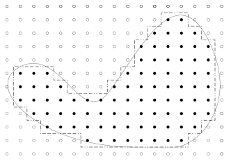
To discretize the continuously defined image I𝐼I in (4) we consider the Gauß discretization Dh(I)subscript𝐷𝐼D_{h}(I), which is the union of the pixels in the descretization of resolution 1h>010\frac{1}{h}>0 with center points in I𝐼I [16]. In the same way, we say that a pixel p𝑝p belongs to a connected component SI𝑆𝐼S\subset I, if its center point lies in S𝑆S (see Fig. 1).

Refer to caption
Figure 1: An object bounded by the black line is discretized into pixels. The center points of the pixels are depicted by dots. The dots \bullet are interior center points with respect to the object, the dots \circ are the exterior center points. The boundary of the discretized object is the dashed line of grid edges.

IV Formulation of the main task: Optimal estimation of the curvature profile

We now consider a digital image, which is a discretized version of the continuous, already segmented image I𝐼I in 4. We assume that we are interested in a certain object in that segmented image. The real, exact object is given by the closed set X[ 0,1]2𝑋superscript 012X\subset[\,0,1\,]^{2}. For example, X𝑋X can be a segmented area or a curve. Our objective is the estimation of the curvature profile along the boundary X𝑋\partial X of X𝑋X, which is the curvature along the curve γ:[a,b][ 0,1]2:𝛾𝑎𝑏superscript 012\gamma:[a,b]\rightarrow[\,0,1\,]^{2} with γ([a,b])=X𝛾𝑎𝑏𝑋\gamma([\,a,b\,])=\partial X. If X𝑋X is a nonempty, bounded, and convex subset of 2superscript2\mathbb{R}^{2} with boundary X𝑋\partial X, and γ𝛾\gamma a curve with grγXgr𝛾𝑋\mathrm{gr\,}\gamma\subset\partial X, then γ𝛾\gamma is called convex.

In the following we define the curvature at the point x=γ(t)𝑥𝛾𝑡x=\gamma(t) with respect to the set X𝑋X by κ(x):=κ(X,x):=κ(t)assign𝜅𝑥𝜅𝑋𝑥assign𝜅𝑡\kappa(x):=\kappa(X,x):=\kappa(t). Then we can pose the problem as follows:

  • Assumptions: We are given a nonempty, connected set of pixels

    Dh(X)Ωh:={Ωh(i,j)}i,jK×J2,subscript𝐷𝑋subscriptΩassignsubscriptsubscriptΩ𝑖𝑗𝑖𝑗𝐾𝐽superscript2D_{h}(X)\subset\Omega_{h}:=\{\Omega_{h}(i,j)\}_{i,j\subset K\times J\subset{\mathbb{Z}}^{2}},

    which is achieved from the Gauß discretization of the object X𝑋X with resolution 1/h11/h.

  • Objective: Optimal estimation of the curvature profile κ(X,x),xX𝜅𝑋𝑥𝑥𝑋\kappa(X,x),\,x\in\partial X, along the boundary X𝑋\partial X of the exact object X𝑋X.

V The MDCA curvature estimator

V-A Definition and Basic Properties of the Maximal Digital Circular Arc (MDCA)

We consider the Minkowski or city-block metric d1subscript𝑑1d_{1}: For two points x=(x1,x2)𝑥subscript𝑥1subscript𝑥2x=(x_{1},x_{2}) and y=(y1,y2)𝑦subscript𝑦1subscript𝑦2y=(y_{1},y_{2}), the metric is defined as

d1(x,y):=|x1y1|+|x2y2|=:xy1.d_{1}(x,y):=|x_{1}-y_{1}|+|x_{2}-y_{2}|=:\|x-y\|_{1}.

In fact, on 2superscript2{\mathbb{R}}^{2} and its subsets, the metric is a norm.

Let (vk)k{1,,N+1}subscriptsubscript𝑣𝑘𝑘1𝑁1(v_{k})_{k\in\{1,\dots,N+1\}} be a finite sequence of grid vertices with vkvk+11=hsubscriptnormsubscript𝑣𝑘subscript𝑣𝑘11\|v_{k}-v_{k+1}\|_{1}=h and vk+2vksubscript𝑣𝑘2subscript𝑣𝑘v_{k+2}\neq v_{k}. We call C=(ek)k{1,,N}𝐶subscriptsubscript𝑒𝑘𝑘1𝑁C=(e_{k})_{k\in\{1,\dots,N\}} with ek=[vk,vk+1]subscript𝑒𝑘subscript𝑣𝑘subscript𝑣𝑘1e_{k}=[v_{k},v_{k+1}] a digital curve (with parameter k𝑘k) of length N𝑁N. e1subscript𝑒1e_{1} is called initial edge of the digital curve; eNsubscript𝑒𝑁e_{N} is the terminal edge.

The distance d𝑑d between two edges eisubscript𝑒𝑖e_{i} and ejsubscript𝑒𝑗e_{j} of a digital curve C=(ek)k=1,,N𝐶subscriptsubscript𝑒𝑘𝑘1𝑁C=(e_{k})_{k=1,\dots,N} is defined by

d(ei,ej):=|ji|assign𝑑subscript𝑒𝑖subscript𝑒𝑗𝑗𝑖d(e_{i},e_{j}):=|j-i|

If C𝐶C is simple (i.e., branching index at most 2 for each point) and closed, we define

d(ei,ej):=min(|ji|,N|ji|)assign𝑑subscript𝑒𝑖subscript𝑒𝑗𝑗𝑖𝑁𝑗𝑖d(e_{i},e_{j}):=\min(|j-i|,N-|j-i|)

Then obviously d(e1,eN)=1𝑑subscript𝑒1subscript𝑒𝑁1d(e_{1},e_{N})=1.

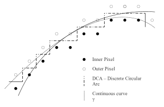
We assume that the boundary Dh(X)subscript𝐷𝑋\partial D_{h}(X) of the Gauß discretized object X𝑋X in our image is a simple closed digital curve Dh(X)subscript𝐷𝑋\partial D_{h}(X). Each edge ekDh(X)subscript𝑒𝑘subscript𝐷𝑋e_{k}\in\partial D_{h}(X) is located between two pixels, an inner pixel pDh(X)𝑝subscript𝐷𝑋p\in D_{h}(X) and an outer pixel qDh(X)𝑞subscript𝐷𝑋q\notin D_{h}(X). Note that the digital curve is needed to be closed only to have the orientation in inner and outer pixels. Since digital curves can be closed in adding appropriate edges, our considerations are not limited to the case of closed curves.

The make use of the following notions of circular separability and digital circular arcs from [11]:

Definition 1.

(Circular separable) Two sets of points P={p1,pN}2𝑃subscript𝑝1subscript𝑝𝑁superscript2P=\{p_{1},\dots p_{N}\}\subset\mathbb{R}^{2} and Q={q1,,qM}2𝑄subscript𝑞1subscript𝑞𝑀superscript2Q=\{q_{1},\dots,q_{M}\}\subset\mathbb{R}^{2} are called circular separable, if there is a radius R0𝑅0R\geq 0 and m2𝑚superscript2m\in\mathbb{R}^{2}, such that for all pP𝑝𝑃p\in P and qQ𝑞𝑄q\in Q it holds that mpRnorm𝑚𝑝𝑅\|m-p\|\leq R and mqRnorm𝑚𝑞𝑅\|m-q\|\geq R (or mpRnorm𝑚𝑝𝑅\|m-p\|\geq R and mqRnorm𝑚𝑞𝑅\|m-q\|\leq R).

Definition 2.

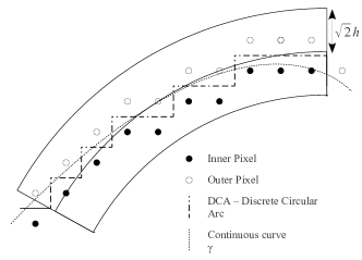
(Digital Circular Arc DCA) Each subset B={ekDh(X)k=1,,N}Dh(X)𝐵conditional-setsubscript𝑒𝑘subscript𝐷𝑋𝑘1𝑁subscript𝐷𝑋B=\{e_{k}\in\partial D_{h}(X)\mid k=1,\dots,N\}\subset\partial D_{h}(X) whose outer pixels and inner pixels are circular separable, is called digital circular arc (DCA).

For our purposes we refine the notion of the digital circular arc in the following way:

Definition 3.

(Maximal Digital Circular Arc MDCA) A digital circular arc ADh(X)𝐴subscript𝐷𝑋A\subset\partial D_{h}(X) is called maximal digital circular arc (MDCA), if every set BDh(X)𝐵subscript𝐷𝑋B\subset\partial D_{h}(X) that contains A𝐴A – i.e. ABDh(X)𝐴𝐵subscript𝐷𝑋A\subset B\subset\partial D_{h}(X) – is not circular separable.

Refer to caption
Figure 2: The digital circular arc (dashed) for the continuous curve γ𝛾\gamma (dotted) separates into inner and outer pixels. For comparison, the separating circle is plotted as continuous curve.

Maximal digital circular arcs satisfy the following properties:

Lemma 4.

[11]

  • (i)

    The set of MDCAs of a given digital curve C𝐶C is unique.

  • (ii)

    Different MDCAs have different sets consisting of the initial and terminal edges.

As a consequence, the MDCAs of a digital curve C=(ek)k=1,,N𝐶subscriptsubscript𝑒𝑘𝑘1𝑁C=(e_{k})_{k=1,\ldots,N} can be ordered with respect to their initial edges, where the parametrization k𝑘k of the digital curve gives the ordering. We denote the ordered sequence of the MDCAs by (Al)l=1,Msubscriptsubscript𝐴𝑙𝑙1𝑀(A_{l})_{l=1,\dots M}, M𝑀M\in{\mathbb{N}}.

V-B Computation of MDCAs and sets of MDCAs

To compute the set of MDCAs one first has to determine for a given digital curve C𝐶C the circular digital arcs. The basic idea of how to do this is as follows: Starting with an edge e𝑒e in C𝐶C one computes a DCA and extends it forward and backward along the edges of the curve C𝐶C until the DCA becomes maximal. The thusly obtained DCA is the first MDCA in the set of MDCAs of C𝐶C. All further elements are computed by choosing the first edge in C𝐶C which is not contained in a previous MDCA and computing the maximal DCA from initial edge onwards.

There exist several optimized algorithms to obtain sets of MDCAs. For a detailed discussion we refer to [17] and the references given therein.

V-C MDCA curvature estimator

Let be given a DCA A=(ek)k=1,,n𝐴subscriptsubscript𝑒𝑘𝑘1𝑛A=(e_{k})_{k=1,\dots,n} in Dh(X)subscript𝐷𝑋\partial D_{h}(X). We denote by Rh(A)superscript𝑅𝐴R^{h}(A) the radius of the smallest separating circle, for which the conditions of Definition 1 holds. We denote by

kh(A):=1/Rh(A),assignsuperscript𝑘𝐴1superscript𝑅𝐴k^{h}(A):=1/R^{h}(A),

the discrete curvature, and by

e(A):=en/2assign𝑒𝐴subscript𝑒𝑛2e(A):=e_{\lceil n/2\rceil}

the central edge of A𝐴A. Here \lceil\cdot\rceil denotes the ceiling function.

Definition 5.

[11] (MDCA curvature estimator) Let (Al)l=1,,Msubscriptsubscript𝐴𝑙𝑙1𝑀(A_{l})_{l=1,\dots,M} be a sequence of MDCAs of a digital curve C𝐶C. Suppose Elsubscript𝐸𝑙E_{l} is a partition of C𝐶C where Elsubscript𝐸𝑙E_{l} is the set of edges eC𝑒𝐶e\in C such that

d(e,e(Al))d(e,e(Ak))k{1,,N}.formulae-sequence𝑑𝑒𝑒subscript𝐴𝑙𝑑𝑒𝑒subscript𝐴𝑘for-all𝑘1𝑁d(e,e(A_{l}))\leq d(e,e(A_{k}))\quad\forall k\in\{1,\dots,N\}.

The MDCA curvature estimator κ^MDCAh(C,e)subscriptsuperscript^𝜅MDCA𝐶𝑒\widehat{\kappa}^{h}_{\text{MDCA}}(C,e) for the digital curve C𝐶C and an edge eEl𝑒subscript𝐸𝑙e\in E_{l} in C𝐶C is defined as the piecewise constant function

κ^MDCAh(C,e):=kh(Al).assignsubscriptsuperscript^𝜅MDCA𝐶𝑒superscript𝑘subscript𝐴𝑙\widehat{\kappa}^{h}_{\text{MDCA}}(C,e):=k^{h}(A_{l}).

For the algorithm, for a given simple closed digital curve C=(ek)k=1,N𝐶subscriptsubscript𝑒𝑘𝑘1𝑁C=(e_{k})_{k=1,\dots N} and grid size h>00h>0 we first compute the set of MDCAs (Al)l=1,,Msubscriptsubscript𝐴𝑙𝑙1𝑀(A_{l})_{l=1,\dots,M} as described in [17]. Denote Rlhsuperscriptsubscript𝑅𝑙R_{l}^{h} the radius of the smallest separating circle of Alsubscript𝐴𝑙A_{l} expressed in terms of the unit hh, and let

Ml:=e(jlil)/2modNassignsubscript𝑀𝑙subscript𝑒modulosubscript𝑗𝑙subscript𝑖𝑙2𝑁M_{l}:=e_{\lceil(j_{l}-i_{l})/2\rceil\!\!\!\!\mod N}

be the set of middle grid edges. For all edges eksubscript𝑒𝑘e_{k} in C𝐶C, k=1,,N𝑘1𝑁k=1,\dots,N, we determine the middle grid edge ei{Mll=1,M}subscript𝑒𝑖conditional-setsubscript𝑀𝑙𝑙1𝑀e_{i}\in\{M_{l}\mid l=1,\ldots M\} which is closest to eksubscript𝑒𝑘e_{k}. Then we set

κ^MDCAh(C,ek)=1/Rih.subscriptsuperscript^𝜅𝑀𝐷𝐶𝐴𝐶subscript𝑒𝑘1superscriptsubscript𝑅𝑖\widehat{\kappa}^{h}_{MDCA}(C,e_{k})=1/R_{i}^{h}.

V-D λ𝜆\lambda-MDCA curvature estimator

We shortly would like to remark on another possible curvature estimator, which we will call λ𝜆\lambda-MDCA curvature estimator. The idea is to consider not only the closest MDCA for an edge eksubscript𝑒𝑘e_{k} of a given curve C𝐶C, but rather all MDCAs in which eksubscript𝑒𝑘e_{k} is contained. The weighting of the contributing curvature estimates is chosen as in [18], where a similar construction was considered for the estimation of tangents.

Definition 6.

Let C=(ek)k={1,,N}𝐶subscriptsubscript𝑒𝑘𝑘1𝑁C=(e_{k})_{k=\{1,\dots,N\}} be a digital arc and let (Al)l{1,,M}subscriptsubscript𝐴𝑙𝑙1𝑀(A_{l})_{l\in\{1,\dots,M\}} be the set of MDCAs of C𝐶C. Denote by eilsubscript𝑒subscript𝑖𝑙e_{i_{l}} and ejlsubscript𝑒subscript𝑗𝑙e_{j_{l}} the start and terminal edges of the MDCA Alsubscript𝐴𝑙A_{l}. For an edge eksubscript𝑒𝑘e_{k} lying on Alsubscript𝐴𝑙A_{l} we define

El(k):=|kiljlil|assignsubscript𝐸𝑙𝑘𝑘subscript𝑖𝑙subscript𝑗𝑙subscript𝑖𝑙E_{l}(k):=\left|\frac{k-i_{l}}{j_{l}-i_{l}}\right|

as the eccentricity of eksubscript𝑒𝑘e_{k} with respect to Alsubscript𝐴𝑙A_{l}.

Obviously, El(k)[0,1]subscript𝐸𝑙𝑘01E_{l}(k)\in[0,1]. The closer El(k)subscript𝐸𝑙𝑘E_{l}(k) approaches 1/2121/2, the closer the edge eksubscript𝑒𝑘e_{k} is lying to the middle edge of the MDCA Alsubscript𝐴𝑙A_{l}.

The idea is now to weight the contribution of the curvatures of the various MDCAs with respect to the eccentricity of the considered edge eksubscript𝑒𝑘e_{k} of C𝐶C. To this end, we consider a continuous concave function λ:[0,1]0+:𝜆01subscriptsuperscript0\lambda:[0,1]\rightarrow\mathbb{R}^{+}_{0} which takes its maximum at the point 1/2121/2 and vanishes at the endpoints of the interval. For example, the functions λ(t):=4t(1t)assign𝜆𝑡4𝑡1𝑡\lambda(t):=4t(1-t) or λ(t):=tlog(t)(1t)log(1t)assign𝜆𝑡𝑡𝑡1𝑡1𝑡\lambda(t):=-t\log(t)-(1-t)\log(1-t) fulfill these requirements.

Definition 7.

(λ𝜆\lambda-MDCA curvature estimator)

Let C=(ek)k={1,,N}𝐶subscriptsubscript𝑒𝑘𝑘1𝑁C=(e_{k})_{k=\{1,\dots,N\}} be a digital curve, (Al)l{1,,n}subscriptsubscript𝐴𝑙𝑙1𝑛(A_{l})_{l\in\{1,\dots,n\}} be the set of MDCAs, and 𝒫(ek):={l:ekAl}assign𝒫subscript𝑒𝑘conditional-set𝑙subscript𝑒𝑘subscript𝐴𝑙\mathcal{P}(e_{k}):=\{l:e_{k}\in A_{l}\}. Let kh(A)superscript𝑘𝐴k^{h}(A) be defined as in Definition 5.

Then

κ^λ-MDCAh(C,ek):=l𝒫(ek)λ(El(k))kh(Al)l𝒫(ek)λ(El(k))assignsubscriptsuperscript^𝜅𝜆-MDCA𝐶subscript𝑒𝑘subscript𝑙𝒫subscript𝑒𝑘𝜆subscript𝐸𝑙𝑘superscript𝑘subscript𝐴𝑙subscript𝑙𝒫subscript𝑒𝑘𝜆subscript𝐸𝑙𝑘\widehat{\kappa}^{h}_{\lambda\text{-MDCA}}(C,e_{k}):=\frac{\sum_{l\in\mathcal{P}(e_{k})}\lambda(E_{l}(k))k^{h}(A_{l})}{\sum_{l\in\mathcal{P}(e_{k})}\lambda(E_{l}(k))}

is the λ𝜆\lambda-MDCA curvature estimator of the digital curve C𝐶C.

In the following section, we prove the convergence of the MDCA curvature estimator, but leave the convergence of the λ𝜆\lambda-MDCA curvature estimator as an open problem. In Section VII, where we discuss experimental results, we will use the λ𝜆\lambda-MDCA curvature estimator for comparison purposes. According these experimental results we conjecture convergence of this weighted estimator with rate comparable to the classical MDCA curvature estimator.

VI Multigrid convergence of the MDCA curvature estimator

In order to obtain error estimates for the MDCA curvature estimator, we first require the concept of multigrid convergence. Multigrid convergence allows the quantification of the error of a discrete geometric estimator when the pixel width gets arbitrarily small, i.e., h00h\to 0.

Discrete geometric estimators are used both to determine global quantities, such as the length of a curve or the area of a surface, as well as local quantities, such as the tangent direction or the curvature of a curve. To the best of our knowledge, up to now, the multigrid convergence of a curvature estimator [12] is an open problem. First estimates are considered in [11] where additional assumptions such as restrictions on the growth of the discrete length of the MDCAs involved. Here, we provide a proof for the uniform multigrid convergence of the MDCA curvature estimator without these assumptions.

VI-A Multigrid convergence

We define the multigrid convergence for local, discrete, geometric estimators.

Let 𝕏𝕏\mathbb{X} be a family of nonempty, compact, simply connected subsets of 2superscript2\mathbb{R}^{2} and let Dh(X)subscript𝐷𝑋\partial D_{h}(X) be a digital curve. A local, discrete, geometric estimator E^=(E^h)h>0^𝐸subscriptsuperscript^𝐸0\widehat{E}=(\widehat{E}^{h})_{h>0} of a local, geometric feature E(X,x)𝐸𝑋𝑥E(X,x) of a set X𝑋X at the point xX𝑥𝑋x\in\partial X is a family of mappings, which assign a real number to a digital curve and an edge on this curve.

Definition 8.

A local, discrete, geometric estimator E^^𝐸\widehat{E} is called multigrid convergent for the family 𝕏𝕏\mathbb{X}, if for all X𝕏𝑋𝕏X\in\mathbb{X}, h>00h>0 and xX𝑥𝑋x\in\partial X the following condition holds:

eDh(X),ye with xy1hformulae-sequencefor-all𝑒subscript𝐷𝑋for-all𝑦𝑒 with subscriptnorm𝑥𝑦1\displaystyle\forall e\in\partial D_{h}(X),\;\forall y\in e\text{ with }\|x-y\|_{1}\leq h
τx(h) with limh0τx(h)=0 such thatsubscript𝜏𝑥 with subscript0subscript𝜏𝑥0 such that\displaystyle\exists\,\tau_{x}(h)\text{ with }\lim_{h\rightarrow 0}\tau_{x}(h)=0\text{ such that}
|E^h(Dh(X),e)E(X,x)|τx(h).superscript^𝐸subscript𝐷𝑋𝑒𝐸𝑋𝑥subscript𝜏𝑥\displaystyle|\widehat{E}^{h}(\partial D_{h}(X),e)-E(X,x)|\leq\tau_{x}(h).

E^^𝐸\widehat{E} is called uniform multigrid convergent if there exists a mapping τ(h)𝜏\tau(h), independent of x𝑥x, with τ(h)τx(h)𝜏subscript𝜏𝑥\tau(h)\geq\tau_{x}(h). τ(h)𝜏\tau(h) is then called the convergence speed.

In the following, we take E^^𝐸\widehat{E} to be the curvature estimator κ^MDCAsubscript^𝜅MDCA\widehat{\kappa}_{\text{MDCA}}, and in addition require that for any X𝕏𝑋𝕏X\in\mathbb{X} the mapping X𝑋\partial X\rightarrow\mathbb{R}, xκ(X,x)maps-to𝑥𝜅𝑋𝑥x\mapsto\kappa(X,x), is continuous.

VI-B Proof of multigrid convergence of the MDCA curvature estimator

Firstly, we define the support function of a convex curve which provide a unique characterization of the curve.

Definition 9.

(Support function)
Let γ:[a,b]2:𝛾𝑎𝑏superscript2\,\gamma:[a,b]\rightarrow\mathbb{R}^{2} be a convex Frenet curve with respect to polar coordinates as in Section II, and let

N(ϕ):=(cosϕsinϕ)assign𝑁italic-ϕitalic-ϕitalic-ϕN(\phi):=\left(\begin{array}[]{c}\cos\phi\\ \sin\phi\end{array}\right)

be its normal. The support function f:=fγMassign𝑓superscriptsubscript𝑓𝛾𝑀f:=f_{\gamma}^{M} of γ𝛾\gamma with center M2𝑀superscript2M\in{\mathbb{R}}^{2} is defined by

fγM(ϕ):[ϕ1,ϕ2],:superscriptsubscript𝑓𝛾𝑀italic-ϕsubscriptitalic-ϕ1subscriptitalic-ϕ2\displaystyle f_{\gamma}^{M}(\phi):\;[\phi_{1},\phi_{2}]\rightarrow\mathbb{R},
fγM(ϕ):=max{γ(t)M,N(ϕ):t[a,b]}assignsuperscriptsubscript𝑓𝛾𝑀italic-ϕ:𝛾𝑡𝑀𝑁italic-ϕ𝑡𝑎𝑏\displaystyle f_{\gamma}^{M}(\phi):=\max\left\{\left<\gamma(t)-M,N(\phi)\right>:t\in[a,b]\right\}

Here ϕ1subscriptitalic-ϕ1\phi_{1} and ϕ2subscriptitalic-ϕ2\phi_{2} is the angle between γ(a)M𝛾𝑎𝑀\gamma(a)-M, resp., γ(b)M𝛾𝑏𝑀\gamma(b)-M and the x𝑥x-axis.

Note that for predefined M𝑀M the support function fγM(ϕ)superscriptsubscript𝑓𝛾𝑀italic-ϕf_{\gamma}^{M}(\phi) determines the curve γ𝛾\gamma completely [19].

In the following, we write f(ϕ):=(fγM)(ϕ):=ddϕfγM(ϕ)assignsuperscript𝑓italic-ϕsuperscriptsuperscriptsubscript𝑓𝛾𝑀italic-ϕassign𝑑𝑑italic-ϕsuperscriptsubscript𝑓𝛾𝑀italic-ϕf^{\prime}(\phi):=\left(f_{\gamma}^{M}\right)^{\prime}(\phi):=\frac{d}{d\phi}f_{\gamma}^{M}(\phi) and f′′(ϕ):=(fγM)′′(ϕ):=d2dϕ2fγM(ϕ)assignsuperscript𝑓′′italic-ϕsuperscriptsuperscriptsubscript𝑓𝛾𝑀′′italic-ϕassignsuperscript𝑑2𝑑superscriptitalic-ϕ2superscriptsubscript𝑓𝛾𝑀italic-ϕf^{\prime\prime}(\phi):=\left(f_{\gamma}^{M}\right)^{\prime\prime}(\phi):=\frac{d^{2}}{d\phi^{2}}f_{\gamma}^{M}(\phi) for the derivatives of the support function.

Lemma 10.

Let γ:[a,b]2:𝛾𝑎𝑏superscript2\gamma:[a,b]\rightarrow\mathbb{R}^{2} be a convex curve as in Definition 9. Let L=(θ2θ1)R𝐿subscript𝜃2subscript𝜃1𝑅L=(\theta_{2}-\theta_{1})R be the central length of the ring segment. Suppose that x¯=γ(ϕ)grγ¯𝑥𝛾italic-ϕgr𝛾\bar{x}=\gamma(\phi)\in\mathrm{gr\,}\gamma. Then,

1κ(x¯)=fγM(ϕ)+(fγM)′′(ϕ).1𝜅¯𝑥superscriptsubscript𝑓𝛾𝑀italic-ϕsuperscriptsuperscriptsubscript𝑓𝛾𝑀′′italic-ϕ\frac{1}{\kappa(\bar{x})}=f_{\gamma}^{M}(\phi)+\left(f_{\gamma}^{M}\right)^{\prime\prime}(\phi).

For the proof, we refer to [19, p. 583].

Definition 11.

For M2𝑀superscript2M\in\mathbb{R}^{2}, R,d+𝑅𝑑superscriptR,d\in\mathbb{R}^{+}, and θ1subscript𝜃1\theta_{1},θ2[0,2π]subscript𝜃202𝜋\theta_{2}\in[0,2\pi], we define a (M,R,d,θ1,θ2)𝑀𝑅𝑑subscript𝜃1subscript𝜃2(M,R,d,\theta_{1},\theta_{2})-ring segment by

\displaystyle\mathcal{R} :=(M,R,d,θ1,θ2)assignabsent𝑀𝑅𝑑subscript𝜃1subscript𝜃2\displaystyle:=\mathcal{R}(M,R,d,\theta_{1},\theta_{2})
:={M+(rcosθ,rsinθ)T|RdrR+d,θ[θ1,θ2]}.assignabsentconditional-set𝑀superscript𝑟𝜃𝑟𝜃𝑇formulae-sequence𝑅𝑑𝑟𝑅𝑑𝜃subscript𝜃1subscript𝜃2\displaystyle:=\left\{M+(r\cos\theta,r\sin\theta)^{T}|R-d\leq r\leq R+d,\theta\in[\theta_{1},\theta_{2}]\right\}.

If for all θ[θ1,θ2]𝜃subscript𝜃1subscript𝜃2\theta\in[\theta_{1},\theta_{2}], the intersection

{M+r(cosθ,sinθ)T|r>0}grγconditional-set𝑀𝑟superscript𝜃𝜃𝑇𝑟0gr𝛾\{M+r(\cos\theta,\sin\theta)^{T}|r>0\}\cap\mathrm{gr\,}\gamma

with a convex curve γ𝛾\gamma consists exactly of one point x(θ)𝑥𝜃x(\theta)\in\mathcal{R}, then one says that the ring segment simply covers γ𝛾\gamma.

Next, we extend Lemma 1 in [11] in the sense that we explicitly give the order of approximation and provide easily verifiable conditions on the convex curve γ𝛾\gamma. To this end, let =(M,R,d,θ1,θ2)𝑀𝑅𝑑subscript𝜃1subscript𝜃2\mathcal{R}=\mathcal{R}(M,R,d,\theta_{1},\theta_{2}) be a ring segment simply covering a convex curve γ𝛾\gamma. We consider a new parameterization of γ𝛾\gamma in terms of θ[θ1,θ2]𝜃subscript𝜃1subscript𝜃2\theta\in[\theta_{1},\theta_{2}]:

x(θ):={M+r(cosθ,sinθ)T|r>0}grγ.assign𝑥𝜃conditional-set𝑀𝑟superscript𝜃𝜃𝑇𝑟0gr𝛾x(\theta):=\{M+r(\cos\theta,\sin\theta)^{T}|r>0\}\cap\mathrm{gr\,}\gamma.

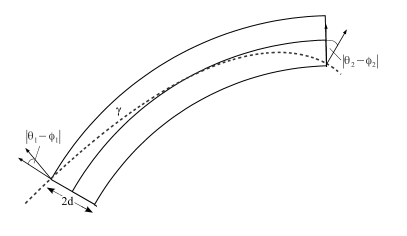
For i=1,2𝑖12i=1,2 the point x(θi)=γ(ϕi)𝑥subscript𝜃𝑖𝛾subscriptitalic-ϕ𝑖x(\theta_{i})=\gamma(\phi_{i}) has normal vector N(ϕi)𝑁subscriptitalic-ϕ𝑖N(\phi_{i}) and grγgr𝛾\mathrm{gr\,}\gamma\cap\mathcal{R} is uniquely characterized by the support function f=fγM:[ϕ1,ϕ2]:𝑓superscriptsubscript𝑓𝛾𝑀subscriptitalic-ϕ1subscriptitalic-ϕ2f=f_{\gamma}^{M}:[\phi_{1},\phi_{2}]\rightarrow\mathbb{R}. (See Figure 3.)

Refer to caption
Figure 3: Simply covering ring segment for the curve γ𝛾\gamma. Note the difference of the angles |θ1ϕ1|subscript𝜃1subscriptitalic-ϕ1|\theta_{1}-\phi_{1}| and |θ2ϕ2|subscript𝜃2subscriptitalic-ϕ2|\theta_{2}-\phi_{2}| of the segment and the normal to the curve γ𝛾\gamma.

In order to state and prove the main theorem, we require some lemmas.

Lemma 12.

Let γ𝛾\gamma be a convex Frenet curve and let \mathcal{R} be a ring segment simply covering γ𝛾\gamma. Suppose that the curvature κ𝜅\kappa of grγgr𝛾\mathrm{gr\,}\gamma\cap\mathcal{R} is bounded below by κmin>0subscript𝜅0\kappa_{\min}>0 and above by κmaxsubscript𝜅\kappa_{\max}. Then the angular difference Δϕ:=ϕ2ϕ1assignΔitalic-ϕsubscriptitalic-ϕ2subscriptitalic-ϕ1\Delta\phi:=\phi_{2}-\phi_{1} is bounded as follows:

κminL(Rd)/RΔϕκmax(L(R+d)/R+4d).subscript𝜅𝐿𝑅𝑑𝑅Δitalic-ϕsubscript𝜅𝐿𝑅𝑑𝑅4𝑑\kappa_{\min}L(R-d)/R\leq\Delta\phi\leq\kappa_{\max}(L(R+d)/R+4d). (5)
Proof.

Let Lγ=Lγ(x(θ1),x(θ2))subscript𝐿𝛾subscript𝐿𝛾𝑥subscript𝜃1𝑥subscript𝜃2L_{\gamma}=L_{\gamma}(x(\theta_{1}),x(\theta_{2})) be the length of γ𝛾\gamma from x(θ1)𝑥subscript𝜃1x(\theta_{1}) to x(θ2)𝑥subscript𝜃2x(\theta_{2}). The convexity of γ𝛾\gamma implies that

(Rd)(θ2θ1)Lγ(R+d)(θ2θ1)+4d,𝑅𝑑subscript𝜃2subscript𝜃1subscript𝐿𝛾𝑅𝑑subscript𝜃2subscript𝜃14𝑑(R-d)(\theta_{2}-\theta_{1})\leq L_{\gamma}\leq(R+d)(\theta_{2}-\theta_{1})+4d,

which is equivalent to

L(Rd)/RLγL(R+d)/R+4d.𝐿𝑅𝑑𝑅subscript𝐿𝛾𝐿𝑅𝑑𝑅4𝑑L(R-d)/R\leq L_{\gamma}\leq L(R+d)/R+4d.

By Eqn. (3) and the convexity of γ𝛾\gamma (i.e. κ>0𝜅0\kappa>0) we have that

Lγ=ϕ1ϕ21κ(γ(ϕ))𝑑ϕ.subscript𝐿𝛾superscriptsubscriptsubscriptitalic-ϕ1subscriptitalic-ϕ21𝜅𝛾italic-ϕdifferential-ditalic-ϕL_{\gamma}=\int_{\phi_{1}}^{\phi_{2}}\frac{1}{\kappa(\gamma(\phi))}d\phi.

As the curvature κ𝜅\kappa is bounded above and below we obtain

κminL(Rd)/RΔϕκmax(L(R+d)/R+4d).subscript𝜅𝐿𝑅𝑑𝑅Δitalic-ϕsubscript𝜅𝐿𝑅𝑑𝑅4𝑑\kappa_{\min}L(R-d)/R\leq\Delta\phi\leq\kappa_{\max}(L(R+d)/R+4d).\qed

The next lemma gives bound on the support function f(ϕ)𝑓italic-ϕf(\phi).

Lemma 13.

Let γ𝛾\gamma be a convex Frenet curve and let \mathcal{R} be a ring segment simply covering γ𝛾\gamma. Suppose that the curvature κ𝜅\kappa is bounded above by κmax>0subscript𝜅0\kappa_{\max}>0. Then the support function f(ϕ)𝑓italic-ϕf(\phi) of γ𝛾\gamma satisfies the estimate

(Rd)(12dκmaxRR+d)f(ϕ)R+d.𝑅𝑑12𝑑subscript𝜅𝑅𝑅𝑑𝑓italic-ϕ𝑅𝑑\displaystyle(R-d)\big{(}1-2d\kappa_{\max}\frac{R}{R+d}\big{)}\leq f(\phi)\leq R+d. (6)
Proof.

For each x(θ)grγ𝑥𝜃gr𝛾x(\theta)\in\mathrm{gr\,}\gamma\cap\mathcal{R} with normal N(ϕ)𝑁italic-ϕN(\phi), we have that f(ϕ)=xMcos|ϕθ|𝑓italic-ϕnorm𝑥𝑀italic-ϕ𝜃f(\phi)=\|x-M\|\cos|\phi-\theta|. Consequently,

(Rd)cos(|ϕθ|)f(ϕ)(R+d).𝑅𝑑italic-ϕ𝜃𝑓italic-ϕ𝑅𝑑\displaystyle(R-d)\cos(|\phi-\theta|)\leq f(\phi)\leq(R+d). (7)

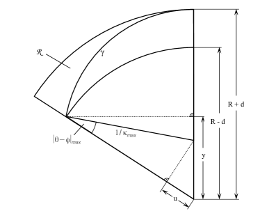
The maximum angle |ϕθ|maxsubscriptitalic-ϕ𝜃|\phi-\theta|_{\max}is obtained if the curve γ𝛾\gamma maintains constant maximum curvature κmaxsubscript𝜅\kappa_{\max} and remains in \mathcal{R}; see Figure 4.

Refer to caption
Figure 4: The curve γ𝛾\gamma in the ring segment \mathcal{R} and the properties of inner and outer radii.

Thus,

cos(|ϕθ|max)=(Rdu)κmaxsubscriptitalic-ϕ𝜃𝑅𝑑𝑢subscript𝜅\cos(|\phi-\theta|_{\max})=(R-d-u)\kappa_{\max}

and

uR+d1/κmax=yRd.𝑢𝑅𝑑1subscript𝜅𝑦𝑅𝑑\frac{u}{R+d-1/\kappa_{\max}}=\frac{y}{R-d}.

Together with

(Rd)2y2=1/κmax2(y(R+d1/κmax))2,superscript𝑅𝑑2superscript𝑦21superscriptsubscript𝜅2superscript𝑦𝑅𝑑1subscript𝜅2(R-d)^{2}-y^{2}=1/\kappa_{\max}^{2}-(y-(R+d-1/\kappa_{\max}))^{2},

this yields

cos(|ϕθ|max)=12Rdκmax/(R+d).subscriptitalic-ϕ𝜃12𝑅𝑑subscript𝜅𝑅𝑑\displaystyle\cos(|\phi-\theta|_{\max})=1-2Rd\kappa_{\max}/(R+d).

Substitution into (7) produces

(Rd)(12Rdκmax/(R+d))f(ϕ)R+d.𝑅𝑑12𝑅𝑑subscript𝜅𝑅𝑑𝑓italic-ϕ𝑅𝑑(R-d)(1-2Rd\kappa_{\max}/(R+d))\leq f(\phi)\leq R+d.\qed

We also need an estimate about the asymptotic behavior with respect to the length Lγsubscript𝐿𝛾L_{\gamma} and the thickness d𝑑d. This estimate is provided by

Lemma 14.

Assume that γ𝛾\gamma is an at least four times differentiable convex curve with ring segment \mathcal{R} which simply covers γ𝛾\gamma. Let γ𝛾\gamma be parametrized by arc length s𝑠s in polar coordinates:

γ(s)=(r(s)cosθ(s),r(s)sinθ(s))T,𝛾𝑠superscript𝑟𝑠𝜃𝑠𝑟𝑠𝜃𝑠𝑇\gamma(s)=(r(s)\cos\theta(s),r(s)\sin\theta(s))^{T},

and let γ(0)𝛾0\gamma(0)\in\mathcal{R}, for all d>0𝑑0d>0. Suppose that the circle 𝒦(M,R)𝒦𝑀𝑅\mathcal{K}(M,R) osculates the curve γ𝛾\gamma at a point x=γ(0)𝑥𝛾0x=\gamma(0), i.e., r(0)=R𝑟0𝑅r(0)=R, r(0)=0superscript𝑟00r^{\prime}(0)=0, and κ(0)=1/R𝜅01𝑅\kappa(0)=1/R. Further suppose that there exists an \ell\in{\mathbb{N}} such that

κ(k)(0)superscript𝜅𝑘0\displaystyle\kappa^{(k)}(0) =0,for k=1,,3,absent0for k=1,,3,\displaystyle=0,\quad\text{for $k=1,\ldots,\ell-3$,} (8)
κ(2)(0)superscript𝜅20\displaystyle\kappa^{(\ell-2)}(0) 0,for 3.absent0for 3.\displaystyle\neq 0,\quad\text{for $\ell\geq 3$.} (9)

Then

d𝒪(Lγ),for Lγ0+.𝑑𝒪superscriptsubscript𝐿𝛾for Lγ0+d\in\mathcal{O}(L_{\gamma}^{\ell}),\quad\text{for $L_{\gamma}\to 0+$}. (10)
Proof.

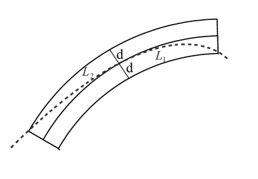
Let γ𝛾\gamma be expressed in polar coordinates with arc length s[L1,L2]𝑠subscript𝐿1subscript𝐿2s\in[-L_{1},L_{2}], where Lγ=L1+L2subscript𝐿𝛾subscript𝐿1subscript𝐿2L_{\gamma}=L_{1}+L_{2}, compare with Figure 5:

γ(s)𝛾𝑠\displaystyle\gamma(s) =(rcosθ,rsinθ)T,absentsuperscript𝑟𝜃𝑟𝜃𝑇\displaystyle=(r\cos\theta,r\sin\theta)^{T},
γ(s)superscript𝛾𝑠\displaystyle\gamma^{\prime}(s) =(rcosθrθsinθ,rsinθ+rθcosθ)T,absentsuperscriptsuperscript𝑟𝜃𝑟superscript𝜃𝜃superscript𝑟𝜃𝑟superscript𝜃𝜃𝑇\displaystyle=(r^{\prime}\cos\theta-r\theta^{\prime}\sin\theta,r^{\prime}\sin\theta+r\theta^{\prime}\cos\theta)^{T},
γ′′(s)superscript𝛾′′𝑠\displaystyle\gamma^{\prime\prime}(s) =(r′′rθ22rθ+rθ′′)cosθ+(2rθrθ′′r′′rθ2)sinθ,absentsuperscript𝑟′′𝑟superscript𝜃22superscript𝑟superscript𝜃𝑟superscript𝜃′′𝜃2superscript𝑟superscript𝜃𝑟superscript𝜃′′superscript𝑟′′𝑟superscript𝜃2𝜃\displaystyle=\left(\begin{array}[]{c}r^{\prime\prime}-r\theta^{\prime 2}\\ 2r^{\prime}\theta^{\prime}+r\theta^{\prime\prime}\end{array}\right)\cos\theta+\left(\begin{array}[]{c}-2r^{\prime}\theta^{\prime}-r\theta^{\prime\prime}\\ r^{\prime\prime}-r\theta^{\prime 2}\end{array}\right)\sin\theta,

which implies

κ𝜅\displaystyle\kappa =γ′′,N(θ)=rθ2r′′.absentsuperscript𝛾′′𝑁𝜃𝑟superscript𝜃2superscript𝑟′′\displaystyle=\langle\gamma^{\prime\prime},N(\theta)\rangle=r\theta^{\prime 2}-r^{\prime\prime}. (11)

Here, γ,r,θ𝛾𝑟𝜃\gamma,r,\theta and all their derivatives are functions in s𝑠s.

Refer to caption
Figure 5: The distance d𝑑d, and the segments L1subscript𝐿1L_{1} and L2subscript𝐿2L_{2} of the curve γ𝛾\gamma (dashed) in the ring segment \mathcal{R}.

Let d(s):=Rr(s)assign𝑑𝑠𝑅𝑟𝑠d(s):=R-r(s), L1sL2subscript𝐿1𝑠subscript𝐿2-L_{1}\leq s\leq L_{2}. In order to use (11), we first need the derivatives of θ(s)𝜃𝑠\theta(s) at s=0𝑠0s=0. As r(0)=0superscript𝑟00r^{\prime}(0)=0, we have θ(0)=ϕ(0)𝜃0italic-ϕ0\theta(0)=\phi(0). Now,

θ(s)superscript𝜃𝑠\displaystyle\theta^{\prime}(s) =dθds(s)=(dθdsθdsθds)(s)absentd𝜃d𝑠𝑠d𝜃dsubscript𝑠𝜃dsubscript𝑠𝜃d𝑠𝑠\displaystyle=\frac{\text{d}\theta}{\text{d}s}(s)=\left(\frac{\text{d}\theta}{\text{d}s_{\theta}}\frac{\text{d}s_{\theta}}{\text{d}s}\right)(s)
=1Rcos(ϕ(s)θ(s))θ(0)=1R,formulae-sequenceabsent1𝑅italic-ϕ𝑠𝜃𝑠superscript𝜃01𝑅\displaystyle=\frac{1}{R}\cdot\cos(\phi(s)-\theta(s))\quad\Rightarrow\quad\theta^{\prime}(0)=\frac{1}{R}, (12)
θ′′(s)superscript𝜃′′𝑠\displaystyle\theta^{\prime\prime}(s) =1Rsin(ϕ(s)θ(s))(ϕ(s)θ(s)),absent1𝑅italic-ϕ𝑠𝜃𝑠superscriptitalic-ϕ𝑠superscript𝜃𝑠\displaystyle=-\frac{1}{R}\cdot\sin(\phi(s)-\theta(s))(\phi^{\prime}(s)-\theta^{\prime}(s)), (13)

implying θ′′(0)=0superscript𝜃′′00\theta^{\prime\prime}(0)=0.

By induction on n𝑛n for n2𝑛2n\geq 2 with initial induction step (13), one can show that

Rθ(n)(s)𝑅superscript𝜃𝑛𝑠\displaystyle R\cdot\theta^{(n)}(s) =cos(ϕ(s)θ(s))×\displaystyle=\cos(\phi(s)-\theta(s))\;\times
2mn1m even1ikn2k=1mik=n1cik(ϕ(ik)(s)θ(ik)(s))subscriptFRACOP2𝑚𝑛1𝑚 evensubscriptproductFRACOP1subscript𝑖𝑘𝑛2superscriptsubscript𝑘1𝑚subscript𝑖𝑘𝑛1subscript𝑐subscript𝑖𝑘superscriptitalic-ϕsubscript𝑖𝑘𝑠superscript𝜃subscript𝑖𝑘𝑠\displaystyle\sum_{2\leq m\leq n-1\atop m\text{ even}}\;\prod_{1\leq i_{k}\leq n-2\atop\sum_{k=1}^{m}i_{k}=n-1}c_{i_{k}}(\phi^{(i_{k})}(s)-\theta^{(i_{k})}(s))
+sin(ϕ(s)θ(s))×\displaystyle+\sin(\phi(s)-\theta(s))\;\times
1mn1m odd 1ikn1k=1mik=n1dik(ϕ(ik)(s)θ(ik)(s)).subscriptFRACOP1𝑚𝑛1𝑚 odd subscriptproductFRACOP1subscript𝑖𝑘𝑛1superscriptsubscript𝑘1𝑚subscript𝑖𝑘𝑛1subscript𝑑subscript𝑖𝑘superscriptitalic-ϕsubscript𝑖𝑘𝑠superscript𝜃subscript𝑖𝑘𝑠\displaystyle\sum_{1\leq m\leq n-1\atop m\text{ odd }}\;\prod_{1\leq i_{k}\leq n-1\atop\sum_{k=1}^{m}i_{k}=n-1}d_{i_{k}}(\phi^{(i_{k})}(s)-\theta^{(i_{k})}(s)).

Condition (2) gives ϕ()(s)=κ(1)(s)superscriptitalic-ϕ𝑠superscript𝜅1𝑠\phi^{(\ell)}(s)=\kappa^{(\ell-1)}(s), and together with (8) we get

θ(n)(0)=0, for 2n1.formulae-sequencesuperscript𝜃𝑛00 for 2𝑛1\displaystyle\theta^{(n)}(0)=0,\quad\text{ for }2\leq n\leq\ell-1. (14)

Now we can calculate the derivatives of d(s)𝑑𝑠d(s) at s=0𝑠0s=0:

d(0)𝑑0\displaystyle d(0) =RR=0,absent𝑅𝑅0\displaystyle=R-R=0,
d(0)superscript𝑑0\displaystyle d^{\prime}(0) =r(0)=0,absentsuperscript𝑟00\displaystyle=-r^{\prime}(0)=0,
d′′(0)superscript𝑑′′0\displaystyle d^{\prime\prime}(0) =r′′(0)=κ(0)θ2(0)r(0)=1R1R2R=0,absentsuperscript𝑟′′0𝜅0superscript𝜃20𝑟01𝑅1superscript𝑅2𝑅0\displaystyle=-r^{\prime\prime}(0)=\kappa(0)-\theta^{\prime 2}(0)r(0)=\frac{1}{R}-\frac{1}{R^{2}}R=0,

where the second-to-last equality holds because of (12). The higher-order derivatives of d𝑑d are obtained again by induction on n𝑛n for n2𝑛2n\geq 2 but with initial induction step d′′(s)=κ(s)θ2(s)r(s)superscript𝑑′′𝑠𝜅𝑠superscript𝜃2𝑠𝑟𝑠d^{\prime\prime}(s)=\kappa(s)-\theta^{\prime 2}(s)r(s):

d(n)(s)superscript𝑑𝑛𝑠\displaystyle d^{(n)}(s) =κ(n2)(s)absentsuperscript𝜅𝑛2𝑠\displaystyle=\kappa^{(n-2)}(s)
1i,jn11kn2i+j+k=ncijkθ(i)(s)θ(j)(s)r(k)(s), for cijk.subscriptformulae-sequence1𝑖𝑗𝑛11𝑘𝑛2𝑖𝑗𝑘𝑛subscript𝑐𝑖𝑗𝑘superscript𝜃𝑖𝑠superscript𝜃𝑗𝑠superscript𝑟𝑘𝑠 for subscript𝑐𝑖𝑗𝑘\displaystyle-\sum_{\begin{subarray}{c}1\leq i,j\leq n-1\\ 1\leq k\leq n-2\\ i+j+k=n\end{subarray}}c_{ijk}\theta^{(i)}(s)\theta^{(j)}(s)r^{(k)}(s),\text{ for }c_{ijk}\in\mathbb{R}.

Using (8) and (14), we thus obtain

d(n)(0)=0, for 0n1,formulae-sequencesuperscript𝑑𝑛00 for 0𝑛1\displaystyle d^{(n)}(0)=0,\quad\text{ for }0\leq n\leq\ell-1, (15)
d()(0)=κ(2)(0)>0.superscript𝑑0superscript𝜅200\displaystyle d^{(\ell)}(0)=\kappa^{(\ell-2)}(0)>0. (16)

Consequently, the Taylor expansion of d(s)𝑑𝑠d(s) at s=0𝑠0s=0 is given by

d(s)=κ(2)(0)!s+o(s), for s0.formulae-sequence𝑑𝑠superscript𝜅20superscript𝑠𝑜superscript𝑠 for 𝑠0d(s)=\frac{\kappa^{(\ell-2)}(0)}{\ell!}\,s^{\ell}+{o}(s^{\ell}),\mbox{ for }s\to 0. (17)

In particular, since |s|max{L1,L2}Lγ𝑠subscript𝐿1subscript𝐿2subscript𝐿𝛾|s|\leq\max\{L_{1},L_{2}\}\leq L_{\gamma}, we have for Lγsubscript𝐿𝛾L_{\gamma} small enough

d𝒪(Lγ), for 3, as Lγ0+.𝑑𝒪superscriptsubscript𝐿𝛾 for 3, as Lγ0+d\in\mathcal{O}(L_{\gamma}^{\ell}),\text{ for $\ell\geq 3$, as $L_{\gamma}\to 0+$}.

Lemma 15.

Suppose the hypotheses of Lemmas 12,13, and 14 are satisfied. Let ϕ¯:=(ϕ1+ϕ2)/2assign¯italic-ϕsubscriptitalic-ϕ1subscriptitalic-ϕ22\bar{\phi}:=(\phi_{1}+\phi_{2})/2.

Then the second derivative of the support function f𝑓f obeys the following asymptotic estimate

|f′′(ϕ¯)|𝒪(dLγ2),as Lγd0+.superscript𝑓′′¯italic-ϕ𝒪𝑑superscriptsubscript𝐿𝛾2as Lγd0+|f^{\prime\prime}(\bar{\phi})|\in\mathcal{O}\left(\frac{d}{L_{\gamma}^{2}}\right),\quad\text{as $L_{\gamma}$, $d\to 0+$}. (18)
Proof.

By induction on the order of derivative of f𝑓f with initial induction step f(3)=(1/κ)f=κ/κ2fsuperscript𝑓3superscript1𝜅superscript𝑓superscript𝜅superscript𝜅2superscript𝑓f^{(3)}=(1/\kappa)^{\prime}-f^{\prime}=\kappa^{\prime}/\kappa^{2}-f^{\prime} (cf. Lemma 10), one can show that for n3𝑛3n\geq 3:

f(n)=(1mn2κ(m+1)1ikn2,i1++im=n2cikmκ(ik))\displaystyle f^{(n)}=\left(\sum_{1\leq m\leq n-2}\kappa^{-(m+1)}\prod_{1\leq i_{k}\leq n-2,\atop i_{1}+\ldots+i_{m}=n-2}c_{i_{k}m}\kappa^{(i_{k})}\right)
f(n2),cikm.superscript𝑓𝑛2subscript𝑐subscript𝑖𝑘𝑚\displaystyle-f^{(n-2)},\qquad c_{i_{k}m}\in\mathbb{R}.

Using condition (8), one obtains

f(k)=f(k2), for all 3k1,formulae-sequencesuperscript𝑓𝑘superscript𝑓𝑘2 for all 3𝑘1f^{(k)}=-f^{(k-2)},\quad\text{ for all }3\leq k\leq\ell-1,\\ (19)

implying that

f(k)=±f′′, for all even k1.formulae-sequencesuperscript𝑓𝑘plus-or-minussuperscript𝑓′′ for all even 𝑘1f^{(k)}=\pm f^{\prime\prime},\quad\text{ for all even }k\leq\ell-1.

The Taylor expansion of f𝑓f at ϕ¯=(ϕ1+ϕ2)/2¯italic-ϕsubscriptitalic-ϕ1subscriptitalic-ϕ22\bar{\phi}=(\phi_{1}+\phi_{2})/2 gives

f(ϕ1)+f(ϕ2)=2f(ϕ¯)+(Δϕ)24f′′(ϕ¯)𝑓subscriptitalic-ϕ1𝑓subscriptitalic-ϕ22𝑓¯italic-ϕsuperscriptΔitalic-ϕ24superscript𝑓′′¯italic-ϕ\displaystyle f(\phi_{1})+f(\phi_{2})=2f(\bar{\phi})+\frac{(\Delta\phi)^{2}}{4}f^{\prime\prime}(\bar{\phi})
+n=4n even(Δϕ)n2n1n!f(n)(ϕ¯),superscriptsubscriptFRACOP𝑛4𝑛 evensuperscriptΔitalic-ϕ𝑛superscript2𝑛1𝑛superscript𝑓𝑛¯italic-ϕ\displaystyle+\sum_{n=4\atop n\text{ even}}^{\infty}\frac{(\Delta\phi)^{n}}{2^{n-1}n!}f^{(n)}(\bar{\phi}),

which together with (19) implies

f(ϕ1)+limit-from𝑓subscriptitalic-ϕ1\displaystyle f(\phi_{1})+ f(ϕ2)=2f(ϕ¯)+(Δϕ)24f′′(ϕ¯)𝑓subscriptitalic-ϕ22𝑓¯italic-ϕsuperscriptΔitalic-ϕ24superscript𝑓′′¯italic-ϕ\displaystyle f(\phi_{2})=2f(\bar{\phi})+\frac{(\Delta\phi)^{2}}{4}f^{\prime\prime}(\bar{\phi})
±n=4n evenl1(Δϕ)n2n1n!f′′(ϕ¯)+n=ln even(Δϕ)n2n1n!f(n)(ϕ¯).plus-or-minussuperscriptsubscriptFRACOP𝑛4𝑛 even𝑙1superscriptΔitalic-ϕ𝑛superscript2𝑛1𝑛superscript𝑓′′¯italic-ϕsuperscriptsubscriptFRACOP𝑛𝑙𝑛 evensuperscriptΔitalic-ϕ𝑛superscript2𝑛1𝑛superscript𝑓𝑛¯italic-ϕ\displaystyle\pm\sum_{n=4\atop n\text{ even}}^{l-1}\frac{(\Delta\phi)^{n}}{2^{n-1}n!}f^{\prime\prime}(\bar{\phi})+\sum_{n=l\atop n\text{ even}}^{\infty}\frac{(\Delta\phi)^{n}}{2^{n-1}n!}f^{(n)}(\bar{\phi}).

Consequently,

f′′(ϕ¯)superscript𝑓′′¯italic-ϕ\displaystyle f^{\prime\prime}(\bar{\phi}) =4(f(ϕ1)2f(ϕ¯)+f(ϕ2))(Δϕ)2±148(Δϕ)4±+𝒪((Δϕ)2)absent4𝑓subscriptitalic-ϕ12𝑓¯italic-ϕ𝑓subscriptitalic-ϕ2plus-or-minussuperscriptΔitalic-ϕ2148superscriptΔitalic-ϕ4𝒪superscriptΔitalic-ϕ2\displaystyle=\frac{4(f(\phi_{1})-2f(\bar{\phi})+f(\phi_{2}))}{(\Delta\phi)^{2}\pm\frac{1}{48}(\Delta\phi)^{4}\pm\dots}+\mathcal{O}((\Delta\phi)^{\ell-2})
=4(f(ϕ1)2f(ϕ¯)+f(ϕ2))(Δϕ)2(1±o((Δϕ)2)+𝒪((Δϕ)2))\displaystyle=\frac{4(f(\phi_{1})-2f(\bar{\phi})+f(\phi_{2}))}{(\Delta\phi)^{2}(1\pm o((\Delta\phi)^{2})}+\mathcal{O}((\Delta\phi)^{\ell-2}))
=4(f(ϕ1)2f(ϕ¯)+f(ϕ2))(Δϕ)2(1o((Δϕ)2)\displaystyle=\frac{4(f(\phi_{1})-2f(\bar{\phi})+f(\phi_{2}))}{(\Delta\phi)^{2}}\,(1\mp o((\Delta\phi)^{2})
+𝒪((Δϕ)2)),for Δϕ0+.\displaystyle\quad+\mathcal{O}((\Delta\phi)^{\ell-2})),\quad\text{for $\Delta\phi\to 0+$.} (20)

Note that the lower bound in (5) shows that Δϕ0+Δitalic-ϕlimit-from0\Delta\phi\to 0+ implies Lγ0+subscript𝐿𝛾limit-from0L_{\gamma}\to 0+, which by (10) implies d0+𝑑limit-from0d\to 0+. Therefore, substituting (5) and (6) into (VI-B), we obtain for Lγ0+subscript𝐿𝛾limit-from0L_{\gamma}\to 0+ and d0+𝑑limit-from0d\to 0+:

|f′′(ϕ¯)|superscript𝑓′′¯italic-ϕ\displaystyle|f^{\prime\prime}(\bar{\phi})| 16R2(R+d+(Rd)Rκmaxκmin2(Rd)2(R+d))×\displaystyle\leq 16\,R^{2}\left(\frac{R+d+(R-d)\,R\kappa_{\max}}{\kappa_{\min}^{2}(R-d)^{2}(R+d)}\right)\;\times
(dLγ2)(1o(Lγ2))+𝒪(Lγ2).𝑑superscriptsubscript𝐿𝛾2minus-or-plus1𝑜superscriptsubscript𝐿𝛾2𝒪superscriptsubscript𝐿𝛾2\displaystyle\quad\left(\frac{d}{L_{\gamma}^{2}}\right)\,\left(1\mp o(L_{\gamma}^{2})\right)+\mathcal{O}(L_{\gamma}^{\ell-2}).

With d𝒪(Lγ)𝑑𝒪superscriptsubscript𝐿𝛾d\in\mathcal{O}(L_{\gamma}^{\ell}) from (10), this gives

|f′′(ϕ¯)|superscript𝑓′′¯italic-ϕ\displaystyle|f^{\prime\prime}(\bar{\phi})| 𝒪(dLγ2)+𝒪(Lγ(2))absent𝒪𝑑superscriptsubscript𝐿𝛾2𝒪superscriptsubscript𝐿𝛾2\displaystyle\in\mathcal{O}\left(\frac{d}{L_{\gamma}^{2}}\right)+\mathcal{O}(L_{\gamma}^{(\ell-2)})
𝒪(dLγ2)(1+𝒪(Lγd))absent𝒪𝑑superscriptsubscript𝐿𝛾21𝒪superscriptsubscript𝐿𝛾𝑑\displaystyle\in\mathcal{O}\left(\frac{d}{L_{\gamma}^{2}}\right)\left(1+\mathcal{O}\left(\frac{L_{\gamma}^{\ell}}{d}\right)\right)
𝒪(dLγ2)(1+𝒪(1))𝒪(dLγ2).absent𝒪𝑑superscriptsubscript𝐿𝛾21𝒪1𝒪𝑑superscriptsubscript𝐿𝛾2\displaystyle\in\mathcal{O}\left(\frac{d}{L_{\gamma}^{2}}\right)\left(1+\mathcal{O}(1)\right)\in\mathcal{O}\left(\frac{d}{L_{\gamma}^{2}}\right).\qed

The next lemma is an extension of Lemma 1 in [11]. Here, we explicitly give an order of approximation.

Lemma 16.

Assume that the hypotheses of Lemmas 12, 13, and 14 are satisfied. Then the following estimate holds for all xgrγ𝑥gr𝛾x\in\mathcal{R}\cap\mathrm{gr\,}\gamma:

|R1/κ(x)|𝒪(dLγ2), as Lγ,d0+.formulae-sequence𝑅1𝜅𝑥𝒪𝑑superscriptsubscript𝐿𝛾2 as subscript𝐿𝛾𝑑limit-from0\displaystyle|R-1/\kappa(x)|\in\mathcal{O}\left(\frac{d}{L_{\gamma}^{2}}\right),\text{ as }L_{\gamma},d\rightarrow 0+.
Proof.

We use Lemma 10. Let x¯grγ¯𝑥gr𝛾\bar{x}\in\mathrm{gr\,}\gamma\cap\mathcal{R} have normal N(ϕ¯)𝑁¯italic-ϕN(\bar{\phi}). Then,

1/κ(x¯)=f(ϕ¯)+f′′(ϕ¯)R+d+𝒪(dLγ2)1𝜅¯𝑥𝑓¯italic-ϕsuperscript𝑓′′¯italic-ϕ𝑅𝑑𝒪𝑑superscriptsubscript𝐿𝛾2\displaystyle 1/\kappa(\bar{x})=f(\bar{\phi})+f^{\prime\prime}(\bar{\phi})\leq R+d+\mathcal{O}\left(\frac{d}{L_{\gamma}^{2}}\right)
\displaystyle\Rightarrow\quad |1/κ(x¯)R|𝒪(dLγ2).1𝜅¯𝑥𝑅𝒪𝑑superscriptsubscript𝐿𝛾2\displaystyle|1/\kappa(\bar{x})-R|\in\mathcal{O}\left(\frac{d}{L_{\gamma}^{2}}\right).

By (8), we have that Lγ0subscript𝐿𝛾0L_{\gamma}\rightarrow 0, and for all xgrγ𝑥gr𝛾x\in\mathrm{gr\,}\gamma\cap\mathcal{R} it follows that xx¯𝑥¯𝑥x\rightarrow\bar{x}, which completes the proof. ∎

Employing the results from the above lemmas, we show that the length Lγsubscript𝐿𝛾L_{\gamma} of the curve γ𝛾\gamma in the ring segment \mathcal{R} does not converge too quickly to 00 when the thickness d0+𝑑limit-from0d\rightarrow 0+. This then implies the convergence of our procedure.

Lemma 17.

Suppose the hypotheses of Lemmas 13 and 14 are satisfied. Then,

d𝒪(Lγ3), for Lγ0+.𝑑𝒪superscriptsubscript𝐿𝛾3 for Lγ0+.d\in\mathcal{O}(L_{\gamma}^{3}),\quad\text{ for $L_{\gamma}\to 0+.$}
Proof.

First, we show that for all d>0𝑑0d>0, there exists an x(θ0)=γ(ϕ0)grγ𝑥subscript𝜃0𝛾subscriptitalic-ϕ0gr𝛾x(\theta_{0})=\gamma(\phi_{0})\in\mathcal{R}\cap\mathrm{gr\,}\gamma with normal N(ϕ0)𝑁subscriptitalic-ϕ0N(\phi_{0}), so that sin(θ0ϕ0)𝒪(d/Lγ)subscript𝜃0subscriptitalic-ϕ0𝒪𝑑subscript𝐿𝛾\sin(\theta_{0}-\phi_{0})\in\mathcal{O}(d/L_{\gamma}) for d0+𝑑limit-from0d\to 0+.

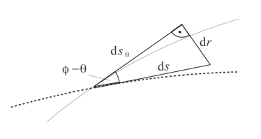
From Figure 6 one deduces that

sin|θϕ|=drdsθ,𝜃italic-ϕ𝑑𝑟𝑑subscript𝑠𝜃\sin|\theta-\phi|=\frac{dr}{ds_{\theta}},

from which it follows that

Lγ(Rd)Rsin(|ϕθ|min)Lγsin(|ϕθ|min)subscript𝐿𝛾𝑅𝑑𝑅subscriptitalic-ϕ𝜃subscript𝐿𝛾subscriptitalic-ϕ𝜃\displaystyle\frac{L_{\gamma}(R-d)}{R}\,\sin(|\phi-\theta|_{\min})\leq L_{\gamma}\,\sin(|\phi-\theta|_{\min})
ϕ1ϕ2sin(|ϕθ|)𝑑sθ=r1r2𝑑r2d.absentsuperscriptsubscriptsubscriptitalic-ϕ1subscriptitalic-ϕ2italic-ϕ𝜃differential-dsubscript𝑠𝜃superscriptsubscriptsubscript𝑟1subscript𝑟2differential-d𝑟2𝑑\displaystyle\leq\int_{\phi_{1}}^{\phi_{2}}\sin(|\phi-\theta|)\,ds_{\theta}=\int_{r_{1}}^{r_{2}}\,dr\leq 2d.

Thus, for d0+𝑑limit-from0d\to 0+,

sin|ϕθ|min2dRLγ(Rd)𝒪(dLγ),subscriptitalic-ϕ𝜃2𝑑𝑅subscript𝐿𝛾𝑅𝑑𝒪subscript𝑑𝐿𝛾\displaystyle\sin|\phi-\theta|_{\min}\leq\frac{2dR}{L_{\gamma}(R-d)}\in\mathcal{O}\left(\frac{d}{L}_{\gamma}\right), (21)

for Lγ0+subscript𝐿𝛾limit-from0L_{\gamma}\to 0+ and d0+𝑑limit-from0d\to 0+. Now, let γ𝛾\gamma be parametrized by arc length s𝑠s, so that x(θ0)=γ(0)𝑥subscript𝜃0𝛾0x(\theta_{0})=\gamma(0). W.l.o.g. assume that r(0)0superscript𝑟00r^{\prime}(0)\leq 0. (Otherwise, we consider the mirror image.) Then sin|θϕ|min=r(0)subscript𝜃italic-ϕsuperscript𝑟0\sin|\theta-\phi|_{\min}=-r^{\prime}(0); see Figure 6.

Refer to caption
Figure 6: Relationship between ds𝑑𝑠ds, dr𝑑𝑟dr and the difference ϕθitalic-ϕ𝜃\phi-\theta. The dotted curve depicts γ𝛾\gamma, the continuous curve shows the central circular curve of the ring segment \mathcal{R}.

The proof of Lemma 14 shows that

κ(s)𝜅𝑠\displaystyle\kappa(s) =θ2(s)r(s)r′′(s),absentsuperscript𝜃2𝑠𝑟𝑠superscript𝑟′′𝑠\displaystyle=\theta^{\prime 2}(s)r(s)-r^{\prime\prime}(s),
d(s)𝑑𝑠\displaystyle d(s) =Rr(s).absent𝑅𝑟𝑠\displaystyle=R-r(s).

Note that

r(s)𝑟𝑠\displaystyle r(s) =r(0)+r(0)s+o(s2)absent𝑟0superscript𝑟0𝑠𝑜superscript𝑠2\displaystyle=r(0)+r^{\prime}(0)s+o(s^{2})
=Rssin|θϕ|min+o(s2),as s0+.absent𝑅𝑠subscript𝜃italic-ϕ𝑜superscript𝑠2as s0+.\displaystyle=R-s\,\sin|\theta-\phi|_{\min}+o(s^{2}),\quad\text{as $s\to 0+$.}

Therefore, for d0+𝑑limit-from0d\to 0+,

d(0)𝑑0\displaystyle d(0) RR+𝒪(d)𝒪(d),absent𝑅𝑅𝒪𝑑𝒪𝑑\displaystyle\in R-R+\mathcal{O}(d)\in\mathcal{O}(d),
d(0)superscript𝑑0\displaystyle d^{\prime}(0) =r(0)=sin|θϕ|min𝒪(dLγ),absentsuperscript𝑟0subscript𝜃italic-ϕ𝒪subscript𝑑𝐿𝛾\displaystyle=-r^{\prime}(0)=\sin|\theta-\phi|_{\min}\in\mathcal{O}\left(\frac{d}{L}_{\gamma}\right),

and

d′′(0)superscript𝑑′′0\displaystyle d^{\prime\prime}(0) =κ(0)θ2(0)r(0)κ(0)1R2(R𝒪(d))absent𝜅0superscript𝜃20𝑟0𝜅01superscript𝑅2𝑅𝒪𝑑\displaystyle=\kappa(0)-\theta^{\prime 2}(0)r(0)\in\kappa(0)-\frac{1}{R^{2}}(R-\mathcal{O}(d))
κ(0)1R+𝒪(d).absent𝜅01𝑅𝒪𝑑\displaystyle\in\kappa(0)-\frac{1}{R}+\mathcal{O}(d).

By Lemma 14, we can write this as

d′′(0)𝒪(dLγ2)+𝒪(d)𝒪(dLγ2).superscript𝑑′′0𝒪𝑑superscriptsubscript𝐿𝛾2𝒪𝑑𝒪𝑑superscriptsubscript𝐿𝛾2\displaystyle d^{\prime\prime}(0)\in\mathcal{O}\left(\frac{d}{L_{\gamma}^{2}}\right)+\mathcal{O}(d)\in\mathcal{O}\left(\frac{d}{L_{\gamma}^{2}}\right).

Therefore, the Taylor expansion of d𝑑d in terms of Lγsubscript𝐿𝛾L_{\gamma} yields

d(Lγ)𝒪(d)+Lγ𝒪(dLγ)+Lγ2𝒪(dLγ2)+𝒪(Lγ3),𝑑subscript𝐿𝛾𝒪𝑑subscript𝐿𝛾𝒪𝑑subscript𝐿𝛾subscriptsuperscript𝐿2𝛾𝒪𝑑superscriptsubscript𝐿𝛾2𝒪superscriptsubscript𝐿𝛾3\displaystyle d(L_{\gamma})\in\mathcal{O}(d)+L_{\gamma}\mathcal{O}\left(\frac{d}{L_{\gamma}}\right)+L^{2}_{\gamma}\mathcal{O}\left(\frac{d}{L_{\gamma}^{2}}\right)+\mathcal{O}(L_{\gamma}^{3}),

which implies the claim for Lγ0+subscript𝐿𝛾limit-from0L_{\gamma}\to 0+.∎

Theorem 18.

Under the same hypotheses and with the same notation as in Lemmas 12, 13, and 14, we obtain for all xgrγ𝑥gr𝛾x\in\mathcal{R}\cap\mathrm{gr\,}\gamma the estimate

|R1κ(x)|𝒪(d1/3).𝑅1𝜅𝑥𝒪superscript𝑑13\left|R-\frac{1}{\kappa(x)}\right|\in\mathcal{O}(d^{1/3}).
Proof.

Substituting the result from Lemma 17 into that of Lemma 14 gives

|R1κ(x)|𝒪(dLγ2)𝒪(dd2/3)𝒪(d1/3).𝑅1𝜅𝑥𝒪𝑑superscriptsubscript𝐿𝛾2𝒪𝑑superscript𝑑23𝒪superscript𝑑13\displaystyle\left|R-\frac{1}{\kappa(x)}\right|\in\mathcal{O}\left(\frac{d}{L_{\gamma}^{2}}\right)\in\mathcal{O}\left(\frac{d}{d^{2/3}}\right)\in\mathcal{O}(d^{1/3}).\qed

The above theorem now implies the uniform multigrid convergence of the curvature estimator κ^MDCAsubscript^𝜅𝑀𝐷𝐶𝐴\widehat{\kappa}_{MDCA}.

Theorem 19.

Suppose 𝕏𝕏\mathbb{X} is a nonempty family of convex and compact subsets of 2superscript2\mathbb{R}^{2}. Further suppose that for all X𝕏𝑋𝕏X\in\mathbb{X} the curvature along the boundary X𝑋\partial X is continuously differentiable, strictly positive, and bounded from above and below by some positive constants.

Then the multigrid curvature estimator κ^MDCAsubscript^𝜅𝑀𝐷𝐶𝐴\widehat{\kappa}_{MDCA} is uniformly multigrid convergent for 𝕏𝕏\mathbb{X} with τ(h)𝒪(h1/3)𝜏𝒪superscript13\tau(h)\in\mathcal{O}(h^{1/3}).

Refer to caption
Figure 7: Illustration of the proof of Theorem 19
Proof.

The original proof can be found in [11]. We reproduce it here in our notation and terminology since it uses arguments that will also be employed in Theorem 20 below, which uses weaker hypotheses.

Assume that X𝕏𝑋𝕏X\in\mathbb{X}, h>00h>0, xX𝑥𝑋x\in\partial X, eDh(X)𝑒subscript𝐷𝑋e\in\partial D_{h}(X) and ye𝑦𝑒y\in e with xy1<hsubscriptnorm𝑥𝑦1\|x-y\|_{1}<h are given. Suppose (Ai)i{1,,n}subscriptsubscript𝐴𝑖𝑖1𝑛(A_{i})_{i\in\{1,\dots,n\}} is the set of MDCAs for Dh(X)subscript𝐷𝑋\partial D_{h}(X). Then y𝑦y is closer to e(Ai)𝑒subscript𝐴𝑖e(A_{i}) than to any other edge. Let 𝒦(m,R)𝒦𝑚𝑅\mathcal{K}(m,R) be the circle with smallest radius that separates the inner pixels {pi}superscript𝑝𝑖\{p^{i}\} and outer pixels {po}superscript𝑝𝑜\{p^{o}\} of Aisubscript𝐴𝑖A_{i}. Let θ1subscript𝜃1\theta_{1} and θ2subscript𝜃2\theta_{2} be the polar angles of the first and last edge of Aisubscript𝐴𝑖A_{i} with respect to the center m𝑚m. Let \mathcal{R} be the associated (m,R,2h,θ1,θ2)𝑚𝑅2subscript𝜃1subscript𝜃2(m,R,\sqrt{2}h,\theta_{1},\theta_{2})-ring. As 𝒦(m,R)𝒦𝑚𝑅\mathcal{K}(m,R) separates the pixels {pi}superscript𝑝𝑖\{p^{i}\} from the pixels {po}superscript𝑝𝑜\{p^{o}\} and d𝑑d was chosen to be equal to 2h2\sqrt{2}h, all these pixels lie inside of \mathcal{R}. Moreover, since X𝑋\partial X lies between {pi}superscript𝑝𝑖\{p^{i}\} and {po}superscript𝑝𝑜\{p^{o}\} it is also contained in \mathcal{R}. It follows from [20] that for small enough h>00h>0 the topologies of Dh(X)subscript𝐷𝑋\partial D_{h}(X) and X𝑋\partial X coincide and thus also those of Dh(X)subscript𝐷𝑋\mathcal{R}\cap\partial D_{h}(X) and X𝑋\mathcal{R}\cap\partial X. Hence, \mathcal{R} simply covers every curve with graph X𝑋\partial X. In addition, x,y𝑥𝑦x,y\in\mathcal{R}. All hypotheses of Theorem 18 are thus satisfied and we can conclude that for all x𝑥x\in\mathcal{R} the following estimate applies:

|κ(X,x)κ^h(Dh(X),e)|=|κ(X,x)1/R|𝜅𝑋𝑥superscript^𝜅subscript𝐷𝑋𝑒𝜅𝑋𝑥1𝑅\displaystyle|\kappa(X,x)-\widehat{\kappa}^{h}(\partial D_{h}(X),e)|=|\kappa(X,x)-1/R|
=|R1/κ(x)||κ(x)/R|𝒪(d1/3)𝒪(h1/3).absent𝑅1𝜅𝑥𝜅𝑥𝑅𝒪superscript𝑑13𝒪superscript13\displaystyle=|R-1/\kappa(x)|\cdot|\kappa(x)/R|\in\mathcal{O}(d^{1/3})\in\mathcal{O}(h^{1/3}).\qed
Theorem 20.

Suppose 𝕏𝕏\mathbb{X} is a nonempty family of compact subsets of 2superscript2\mathbb{R}^{2}. Further suppose that for all X𝕏𝑋𝕏X\in\mathbb{X} the curvature along the boundary X𝑋\partial X is bounded above and below by some positive constants. If the function xκ(X,x)maps-to𝑥𝜅𝑋𝑥x\mapsto\kappa(X,x) is continuously differentiable at x0subscript𝑥0x_{0}, x0Xfor-allsubscript𝑥0𝑋\forall\,x_{0}\in\partial X with κ(X,x0)0𝜅𝑋subscript𝑥00\kappa(X,x_{0})\neq 0, then eDh(X)for-all𝑒subscript𝐷𝑋\forall e\in\partial D_{h}(X) and yefor-all𝑦𝑒\forall y\in e with x0y1hsubscriptnormsubscript𝑥0𝑦1\|x_{0}-y\|_{1}\leq h, the following estimate holds:

|κ^h(Dh(X),e)κ(X,x0)|𝒪(h1/3).superscript^𝜅subscript𝐷𝑋𝑒𝜅𝑋subscript𝑥0𝒪superscript13\displaystyle|\widehat{\kappa}^{h}(\partial D_{h}(X),e)-\kappa(X,x_{0})|\in\mathcal{O}(h^{1/3}).
Proof.

Assume that X𝕏𝑋𝕏X\in\mathbb{X} and x0Xsubscript𝑥0𝑋x_{0}\in\partial X are satisfying the hypotheses set forth in the theorem. Moreover, for an h>00h>0, let eDh(X)𝑒subscript𝐷𝑋e\in D_{h}(X) and ye𝑦𝑒y\in e with x0y1<hsubscriptnormsubscript𝑥0𝑦1\|x_{0}-y\|_{1}<h be given. As in the proof of Theorem 19 we define an (m,R,2h,θ1,θ2)𝑚𝑅2subscript𝜃1subscript𝜃2(m,R,\sqrt{2}h,\theta_{1},\theta_{2})-ring hsuperscript\mathcal{R}^{h} depending on hh. As κ(X,x0)0𝜅𝑋subscript𝑥00\kappa(X,x_{0})\neq 0 and the mapping xκ(X,x)maps-to𝑥𝜅𝑋𝑥x\mapsto\kappa(X,x) is continuously differentiable at x0subscript𝑥0x_{0}, there exists a neighborhood U𝑈U of x0subscript𝑥0x_{0} such that UX𝑈𝑋U\cap\partial X is the graph of a convex curve with strictly positive or negative curvature. Assume w.l.o.g. that the curvature is strictly positive. From Lemma 14 we infer that the length of a maximal digital arc goes to zero as h00h\to 0. Therefore, there exists an h0>0subscript00h_{0}>0 so that for all hh0subscript0h\leq h_{0} the intersection hXsuperscript𝑋\mathcal{R}^{h}\cap\partial X is the graph of a convex curve with strictly positive and continuously differentiable curvature. The claim now follows from the arguments given in the proof of Theorem 19. ∎

VII Experimental valuation

In this section, we evaluate the MDCA and λ𝜆\lambda–MDCA curvature estimator. For this purpose, we use the following four segmented test objects, i.e., planar curves for which the exact curvature profiles can be computed explicitly. Except for the ellipse, these planar curves are not globally convex. However, they are taken as piecewise convex curves. In concave regions, we consider the inversely parametrized curve.

Refer to caption
(a) Ellipse
Refer to caption
(b) Gummy Bear
Refer to caption
(c) Hour Glass
Refer to caption
(d) Rhombus
Figure 8: Test Objects (a)–(b) fulfill the requirements of Theorem 20, whereas (d) does not, since it has corners.

The first test object (a) is an ellipse

E:={(xy)2x2a2+y2b2=1}assign𝐸conditional-setFRACOP𝑥𝑦superscript2superscript𝑥2superscript𝑎2superscript𝑦2superscript𝑏21E:=\left\{\left({{x}\atop{y}}\right)\in\mathbb{R}^{2}\;\mid\;\frac{x^{2}}{a^{2}}+\frac{y^{2}}{b^{2}}=1\right\}

with semi axes a=9𝑎9a=9 and b=3𝑏3b=3. The second test object, which was termed “gummy bear,” is represented by the point set

G:={(xy)2(x3)4+(y2)4x2y2=1},assign𝐺conditional-setFRACOP𝑥𝑦superscript2superscript𝑥34superscript𝑦24superscript𝑥2superscript𝑦21\displaystyle G:=\left\{\left({{x}\atop{y}}\right)\in\mathbb{R}^{2}\;\mid\;\left(\frac{x}{3}\right)^{4}+\left(\frac{y}{2}\right)^{4}-x^{2}-y^{2}=1\right\},

and the third object, named “hour glass,” by the point set

S:=assign𝑆absent\displaystyle S:= {(xy)2|(3.96+(x3)2+(y3)2)215.84(x3)2=16}.conditional-setFRACOP𝑥𝑦superscript2superscript3.96superscript𝑥32superscript𝑦32215.84superscript𝑥3216\displaystyle\left\{\left({{x}\atop{y}}\right)\in{\mathbb{R}}^{2}\;|\;\left(3.96+\left(\frac{x}{3}\right)^{2}+\left(\frac{y}{3}\right)^{2}\right)^{2}-15.84\cdot\left(\frac{x}{3}\right)^{2}=16\right\}.

We consider the object (d), the rhombus, in more detail in Section VII-B.

The exact curvature profile along the curve γXsubscript𝛾𝑋\gamma_{X} with graph grγX=Xgrsubscript𝛾𝑋𝑋\mathrm{gr\,}\gamma_{X}=X for the each test object X{E,G,S}𝑋𝐸𝐺𝑆X\in\{E,G,S\} can be explicitly computed by means of the following formula (see, e.g. [13, 14, 15]):

κ=gxxgy2gxygxgy+gyygx(gx2+gy2)3/2,𝜅subscript𝑔𝑥𝑥subscript𝑔𝑦2subscript𝑔𝑥𝑦subscript𝑔𝑥subscript𝑔𝑦subscript𝑔𝑦𝑦subscript𝑔𝑥superscriptsuperscriptsubscript𝑔𝑥2superscriptsubscript𝑔𝑦232\displaystyle\kappa=\frac{g_{xx}g_{y}-2g_{xy}g_{x}g_{y}+g_{yy}g_{x}}{(g_{x}^{2}+g_{y}^{2})^{3/2}},

where X𝑋X satisfies the implicit equation g(x,y)=0𝑔𝑥𝑦0g(x,y)=0.

VII-A Experimental Error

The four test objects are Gauß–discretized (see Section III) using h=2nsuperscript2𝑛\,h=2^{-n} with n{0,,6}𝑛06n\in\{0,\dots,6\}. Next, the MDCA and λ𝜆\lambda–MDCA curvature estimators are computed and compared to the exact curvature calculation. In order to compare the error at pixel edge e𝑒e with the exact value, we consider the point p=(x,y)TXsuperscript𝑝superscriptsuperscript𝑥superscript𝑦𝑇𝑋p^{\prime}=(x^{\prime},y^{\prime})^{T}\in\partial X whose distance to the midpoint of e𝑒e is minimal. The absolute error at e𝑒e for resolution hh is then given by

ϵabsh(e):=|κ(X,p)κ^MDCAh(Dh(X),e)|.assignsuperscriptsubscriptitalic-ϵabs𝑒𝜅𝑋superscript𝑝superscriptsubscript^𝜅MDCAsubscript𝐷𝑋𝑒\displaystyle\epsilon_{\mathrm{abs}}^{h}(e):=|\kappa(X,p^{\prime})-\widehat{\kappa}_{\mathrm{MDCA}}^{h}(\partial D_{h}(X),e)|.

We define the average error by

ϵavh:=1|Dh(X)|eDh(X)ϵabsh(e).assignsuperscriptsubscriptitalic-ϵav1subscript𝐷𝑋subscript𝑒subscript𝐷𝑋superscriptsubscriptitalic-ϵabs𝑒\displaystyle\epsilon_{\mathrm{av}}^{h}:=\frac{1}{|D_{h}(X)|}\sum_{e\in D_{h}(X)}\epsilon_{\mathrm{abs}}^{h}(e).

Here, |Dh(X)|subscript𝐷𝑋|D_{h}(X)| denotes the number of edges of the simple closed digital curve whose graph is Dh(X)subscript𝐷𝑋D_{h}(X). Furthermore, we define the maximal error as

ϵmaxh:=maxeDh(X)ϵabsh(e).assignsuperscriptsubscriptitalic-ϵsubscript𝑒subscript𝐷𝑋superscriptsubscriptitalic-ϵabs𝑒\displaystyle\epsilon_{\mathrm{\max}}^{h}:=\max_{e\in D_{h}(X)}\epsilon_{\mathrm{abs}}^{h}(e).

In Figures 9 and 10 the average and maximal errors are plotted against the resolution hh. The plots are double logarithmically scaled. Using this particular scaling of the axes, we see that the slope of the regression line for the error values equals the experimental speed of convergence:

log(ϵ)=mlog(h)+Citalic-ϵ𝑚𝐶\displaystyle\log(\epsilon)=m\cdot\log(h)+{C} log(ϵ)=log(hm)+Cabsentitalic-ϵsuperscript𝑚𝐶\displaystyle\Longleftrightarrow\log(\epsilon)=\log(h^{m})+{C}
ϵ=Chm,absentitalic-ϵ𝐶superscript𝑚\displaystyle\Longleftrightarrow\epsilon={C}\cdot h^{m},

where C𝐶C\in{\mathbb{R}}.

Refer to caption
Figure 9: Average Error for the MDCA and the λ𝜆\lambda-MDCA curvature estimators evaluated at the smooth test objects for varying pixel width hh.
Refer to caption
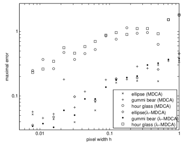
Figure 10: Maximal Error for the MDCA and the λ𝜆\lambda-MDCA curvature estimators evaluated at the smooth test objects for varying pixel width hh. The λ𝜆\lambda-MDCA curvature estimator shows a higher order of convergence than the standard MDCA-estimator; compare also with Table I.

The plots indicate that for the average error there is hardly any difference between the λ𝜆\lambda–MDCA and the MDCA curvature estimator. However, when the maximum error is considered the λ𝜆\lambda–MDCA curvature estimator exhibits a faster speed of convergence. For the calculations, the weight function λ(t)=tlog(t)(1t)log(1t)𝜆𝑡𝑡𝑡1𝑡1𝑡\lambda(t)=-t\log(t)-(1-t)\log(1-t) was used.

The experimental convergence speeds for the three test objects are summarized in Table I. One observes the following: Firstly, the convergence of the maximal error for the test object “hour glass” is the slowest with 𝒪(h0.36)𝒪superscript0.36\mathcal{O}(h^{0.36}) and this value is already close to the theoretical limit of 𝒪(h13)𝒪superscript13\mathcal{O}(h^{\frac{1}{3}}). Secondly, the convergence of the average error for the test object “ellipse” is even faster than 𝒪(h)𝒪\mathcal{O}(h).

Ellipse Gummy Bear Hour Glass
Avg. Error (MDCA) 𝒪(h1.08)𝒪superscript1.08\mathcal{O}(h^{1.08}) 𝒪(h0.64)𝒪superscript0.64\mathcal{O}(h^{0.64}) 𝒪(h0.57)𝒪superscript0.57\mathcal{O}(h^{0.57})
Max. Error (MDCA) 𝒪(h0.44)𝒪superscript0.44\mathcal{O}(h^{0.44}) 𝒪(h0.42)𝒪superscript0.42\mathcal{O}(h^{0.42}) 𝒪(h0.36)𝒪superscript0.36\mathcal{O}(h^{0.36})
Avg. Error (λ𝜆\lambda-MDCA) 𝒪(h1.06)𝒪superscript1.06\mathcal{O}(h^{1.06}) 𝒪(h0.68)𝒪superscript0.68\mathcal{O}(h^{0.68}) 𝒪(h0.56)𝒪superscript0.56\mathcal{O}(h^{0.56})
Max. Error (λ𝜆\lambda-MDCA) 𝒪(h0.50)𝒪superscript0.50\mathcal{O}(h^{0.50}) 𝒪(h0.56)𝒪superscript0.56\mathcal{O}(h^{0.56}) 𝒪(h0.37)𝒪superscript0.37\mathcal{O}(h^{0.37})
Table I: Experimental Speed of Convergence

VII-B Limits of the Method

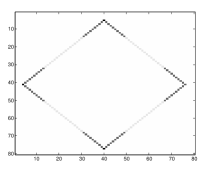
A test object for which the MDCA curvature estimator performs very badly is the rhombus (see Figure 8 (d)). It is represented by the point set

Q:={(x,y)T2||x|+|y|9}.assign𝑄conditional-setsuperscript𝑥𝑦𝑇superscript2𝑥𝑦9Q:=\{(x,y)^{T}\in{\mathbb{R}}^{2}\;|\;|x|+|y|\leq 9\}.

Every boundary point of the set Q𝑄Q was excluded in Theorem 20: At the four corners of the rhombus, the curvature is not defined, i.e., unbounded, and for the remaining boundary points the curvature is equal to zero. Hence, it is not possible to employ Theorem 20 to prove convergence to the actual curvature κ(Q,x)𝜅𝑄𝑥\kappa(Q,x). This is illustrated in Figure 11 which shows that for a resolution of h=22superscript22h=2^{-2} the curvature is badly approximated in a neighborhood of the corners.

The reason for this discrepancy lies in the fact that the entire side of the rhombus is one MDCA and that the midpoint of the subsequent MDCA is located next to the corner. Hence, all points on the side of the rhombus that are closer to a corner than to the midpoint of the side use the MDCA at the corner. For this MDCA, however, the curvature is substantially larger than zero. From the mathematical point of view, the curvature of the rhombus is not bounded below by a positive constant, thus the requirements of Theorem 20 are not met.

The λ𝜆\lambda–MDCA curvature estimator circumvents this problem by assigning higher weights to the digital arcs when a boundary point moves to a more central position. As an MDCA at the side of the rhombus is significantly longer than one at a corner, it is weighted higher and therefore a better result is obtained; see Figure 12.
Refer to caption
(a) Graphical Representation
Refer to caption
(b) Curvature Profile
Figure 11: MDCA Curvature Estimator for the Rhombus
Refer to caption
(a) Graphical Representation
Refer to caption
(b) Curvature Profile
Figure 12: λ𝜆\lambda–MDCA Curvature Estimator for the Rhombus

VIII Conclusion

We analyzed the parameter-free MDCA curvature estimator presented in [11], which is based on maximal digital circular arcs (MDCA). In addition, we extended this estimator to the new λ𝜆\lambda-MDCA curvature estimator, which is smoother and does also not require any parameter. Especially around corners this estimator provides better results then the MDCA estimator.

For convex sets with positive, continuous curvature profile we provided a proof for its uniform multigrid convergence as defined in [21] with convergence speed of 𝒪(h13)𝒪superscript13\mathcal{O}(h^{\frac{1}{3}}). In an experimantal evaluation we observed that this speed of convergence is almost reached for some sets and therefore seems to be the optimal upper bound.

The respective results on the optimal multigrid convergence rate for λ𝜆\lambda-MDCA curvature estimator are still an open question.

References

  • [1] I. T. Young, J. E. Walker, and J. E. Bowie, “An analysis technique for biological shape. i,” Information and Control, vol. 25, no. 4, pp. 357–370, 1974.
  • [2] P. B. Canham, “The minimum energy of bending as a possible explanation of the biconcave shape of the human red blood cell,” Journal of Theoretical Biology, vol. 26, no. 1, pp. 61–76, January 1970.
  • [3] L. J. van Vliet and P. W. Verbeek, “Curvature and bending energy in digitized 2d and 3d images,” in Proceedings of the 8th Scandinavian Conference on Image Analysis (SCIA), 1993, pp. 1403–1410.
  • [4] J. S. Duncan, F. A. Lee, A. W. M. Smeulders, and B. L. Zaret, “A bending energy model for measurement of cardiac shape deformity,” IEEE Transactions on Medical Imaging, vol. 10, no. 3, pp. 307–320, 1991.
  • [5] A. Pasqualato, A. Palombo, A. Cucina, M. Mariggiò, L. Galli, D. Passaro, S. Dinicola, S. Proietti, F. D’Anselmi, P. Coluccia, and M. Bizzarri, “Quantitative shape analysis of chemoresistant colon cancer cells: Correlation between morphotype and phenotype,” Experimental Cell Research, vol. 318, no. 7, pp. 835–846, 2012.
  • [6] R. Marcondes Cesar, Jr. and L. da Fontoura Costa, “Application and assessment of multiscale bending energy for morphometric characterization of neural cells,” Rev. Sci. Instrum., vol. 68, no. 5, pp. 2177–2186, May 1997.
  • [7] A. Backhaus, A. Kuwabara, M. Bauch, N. Monk, G. Sanguinetti, and A. Fleming, “Leafprocessor: a new leaf phenotyping tool using contour bending energy and shape cluster analysis.” New Phytologist, vol. 187, pp. 251–261, 2010.
  • [8] A. J. Sodt and R. W. Pastor, “Bending free energy from simulation: Correspondence of planar and inverse hexagonal lipid phases,” Biophys J., vol. 104, no. 10, pp. 2202–2211, May 2013.
  • [9] G. G. Gordon, “Face recognition based on depth and curvature features,” IEEE Computer Society Conference on Computer Vision and Pattern Recognition, pp. 808–810, 1992.
  • [10] A. C. Jalba, M. H. F. Wilkinson, J. B. T. M. Roerdink, M. M. Bayer, and S. Juggins, “Automatic diatom identification using contour analysis by morphological curvature scale spaces,” Machine Vision and Applications, vol. 16, no. 4, pp. 217–22, 2005.
  • [11] T. Roussillon and J.-O. Lachaud, “Accurate curvature estimation along digital contours with maximal digital circular arcs,” Combinatorial Image Analysis, vol. 6636, pp. 43–55, 2011.
  • [12] D. Coeurjolly, J. Lachaud, and T. Roussillon, “Multigrid convergence of discrete geometric estimators,” Digital Geometry Algorithms, vol. 2, pp. 395–424, 2012.
  • [13] M. Do Carmo, Differential Geometry of Curves and Surfaces.   Pearson, 1976.
  • [14] W. Kühnel, Differentialgeometrie, 5th ed.   Vieweg+Teubner, 2010.
  • [15] S. Montiel and A. Ros, Curves and Surfaces, 2nd ed.   AMS, 2009.
  • [16] R. Klette and A. Rosenfeld, Digital geometry—Geometric Methods for Digital Picture Analysis.   Morgan Kaufmann Publishers, 2004.
  • [17] T. Roussillon, L. Tougne, and I. Sivignon, “On three constrained versions of the digital circular arc recognition problem,” in DGCI 2009, ser. LNCS 5810, S. Brlek, C. Rautenauer, and X. Provençal, Eds.   Berlin Heidelberg: Springer-Verlag, 2009, pp. 34–45.
  • [18] J. Lachaud, A. Vialard, and F. de Vieilleville, “Fast, accurate and convergent tangent estimation on digital contours,” Image and Vision Computing, vol. 25, no. 10, pp. 1572–1587, 2007.
  • [19] H. Flanders, “A proof of Minkowski’s inequality for convex curves,” The American Mathematical Monthly, vol. 75, pp. 581–593, 1968.
  • [20] A. Gross and L. Latecki, “Digitizations preserving topological and differential geometric properties,” Computer Vision and Image Understanding, vol. 62, no. 3, pp. 370–381, 1995.
  • [21] R. Klette, “Multigrid convergence of geometric features,” in Digital and Image Geometry, ser. Lecture Notes in Computer Science, G. Bertrand, A. Imiya, and R. Klette, Eds.   Springer, 2001, vol. 2243, pp. 318–338.