Sterile neutrinos in the light of IceCube

Abstract

We determine constraints on parameters of a single eV-scale light neutrino using IceCube-59 data. Particular emphasis is put on the question whether such an analysis can rule out sterile neutrino hints. While important complementary information is provided, the different dependence on the various sterile neutrino mixing angles makes it currently not possible to fully exclude short baseline appearance results or sterile neutrinos in general.

I Introduction

Though the standard 3-neutrino mixing paradigm has been well established Olive et al. (2014), there are still several short-baseline anomalies, most notably in LSND Aguilar-Arevalo et al. (2001), MiniBooNE Aguilar-Arevalo et al. (2013) and reactor neutrino flux measurements Mueller et al. (2011); Huber (2011). These anomalies could be explained by introducing light sterile neutrinos with the mass-squared difference $\Delta m^{2}$ at $0.1\sim 1\,{\rm eV}^{2}$ scale and mixing matrix elements around 0.1. If such light sterile neutrinos would indeed exist, the theoretical implications would be profound. Therefore several experiments are running or in construction in order to confirm or refuse the existence of light sterile neutrinos. See the recent reviews Abazajian et al. (2012); Gariazzo et al. (2015) for an overview of the hints, consequences and tests of light sterile neutrinos.

In this work we focus on effects of eV-scale sterile neutrinos in atmospheric neutrino oscillations at high energies as measured in the IceCube experiment. We use here an IceCube-59 data set from Ref. Aartsen et al. (2014), where a search for diffuse astrophysical neutrinos was performed. The fact that sterile neutrinos would have an impact in IceCube is easily understood by noting that a mass-squared difference of order eV² corresponds to maximal oscillations at energies $E_{\nu}\sim 10^{3}$ GeV and a baseline around Earth radius $R_{\oplus}\simeq 6.4\times 10^{3}$ km. Indeed, atmospheric neutrinos observed in IceCube have energies ranging from $10^{2}$ GeV to $10^{6}$ GeV, peaked at about $10^{3}$ GeV. Several papers have in the past analyzed the effect of light sterile neutrinos at high energies as a potential test of the sterile neutrino hypothesis Nunokawa et al. (2003); Choubey (2007); Razzaque and Smirnov (2011); Barger et al. (2012); Esmaili et al. (2012, 2013); Esmaili and Smirnov (2013); Arguelles and Kopp (2012).

We will perform here a $\chi^{2}$-analysis on the IceCube-59 data within a $3+1$ scheme to see how significant the constraint on sterile neutrinos is. We are particularly interested in the interplay of this constraint with the results of short baseline appearance and other experiments. We work in the minimal framework of only one sterile neutrino with a unitary $4\times 4$ matrix and no additional interactions. Even in this simple situation the dependence on the various lepton mixing angles is different in each experiment, and in addition, muon neutrino disappearance in IceCube depends on the weakly constrained angle $\theta_{34}$, that should not be set to zero in analyses. For scenarios with more than one sterile state the larger number of mixing angles will complicate further the direct comparison of oscillation probabilities in IceCube and other experiments. Moreover, there is dependence on the sterile neutrino global fit results to which one compares the IceCube sensitivity. All in all, a full exclusion of short baseline appearance and/or other results is currently not possible, though of course important complementary constraints on sterile neutrinos are provided by IceCube data.

The paper is build up as follows: in Section II we discuss the procedure to obtain the oscillation probability of high energy neutrinos including matter effects, before discussing event numbers in IceCube in Section III. The numerical analysis of IceCube data is performed in Section IV, where we also discuss the comparison of the parameters crucial for IceCube with the ones for short baseline appearance and other experiments.

II Atmospheric neutrino disappearance induced by sterile neutrinos

Neutrino oscillation can be described by the following Schrödinger equation in flavor space,

$$i\frac{d}{dL}|\nu(L)\rangle=H|\nu(L)\rangle,$$ (1)

where $H$ is the effective Hamiltonian and $|\nu(L)\rangle$ denotes the flavor state of the neutrino at a distance of $L$ from the source. For the standard 3+1 neutrino framework with 3 active neutrinos $(\nu_{e},\nu_{\mu},\nu_{\tau})$ plus one sterile neutrino $\nu_{s}$, including matter effects, the effective Hamiltonian $H$ has the following matrix form

$$H=\frac{1}{2E}U\left(\begin{array}[]{cccc}m_{1}^{2}\\ &m_{2}^{2}\\ &&m_{3}^{2}\\ &&&m_{4}^{2}\end{array}\right)U^{\dagger}+\sqrt{2}G_{F}N_{e}\left(\begin{array}[]{cccc}1\\ &0\\ &&0\\ &&&\kappa\end{array}\right).$$ (2)

Here $E$ is the neutrino energy, $m_{i}$ and $U$ are the neutrino masses and mixing matrix; $G_{F}$ is the Fermi constant, $N_{e}$ is the electron number density of matter and $\kappa$ is a ratio defined as

$$\kappa\equiv\frac{N_{n}}{2N_{e}}\,,$$ (3)

where $N_{n}$ is the neutron number density. For anti-neutrinos, we need to replace $U\rightarrow U^{*}$ and $G_{F}N_{e}\rightarrow-G_{F}N_{e}$ in Eq. (2).

For constant matter density, $H$ does not vary with $L$ so the solution is simply $|\nu(L)\rangle=e^{-iHL}|\nu(0)\rangle$. But the matter density of Earth Dziewonski and Anderson (1981) varies significantly from $1\,\rm g/{\rm cm}^{3}$ (at the surface) to $13\,\rm g/{\rm cm}^{3}$ (at the inner core), so that to obtain accurate results one has to either numerically solve the full differential equation Eq. (1), or divide the full neutrino path into many segments with approximated constant densities so that

$$|\nu(L)\rangle=\prod_{i}e^{-iH_{i}L_{i}}|\nu(0)\rangle\,.$$ (4)

Here $H_{i}$ is the Hamiltonian in the $i$-th segment and $L_{i}$ is the corresponding baseline. Actually this is the main method used to compute oscillation probabilities in the GLoBES package Huber et al. (2007) (see also Wallraff and Wiebusch (2014)). In this work, we will adopt the same method, i.e. Eq. (4), to compute probabilities. Defining the $S$-matrix as

$$S_{\alpha\beta}\equiv\left(\prod_{i}e^{-iH_{i}L_{i}}\right)_{\alpha\beta}\,,$$ (5)

where $\alpha$, $\beta$ are flavor indices ($e$, $\mu$, $\tau$ and $s$), the survival probability of $\nu_{\mu}$ is given by

$$P_{\nu_{\mu}\rightarrow\nu_{\mu}}=|S_{\mu\mu}|^{2}\,.$$ (6)

For the energy range of IceCube, $\nu_{\mu}$ and $\overline{\nu}_{\mu}$ dominate the atmospheric neutrino flux while $\nu_{e}$ and $\overline{\nu}_{e}$ are negligible; thus only $P_{\nu_{\mu}\rightarrow\nu_{\mu}}$ and $P_{\overline{\nu}_{\mu}\rightarrow\overline{\nu}_{\mu}}$ will be used in this work. The $4\times 4$ mixing matrix is

$$U=R^{34}R^{24}R^{14}R^{23}R^{13}R^{12}\,,$$

where $R^{ij}$ is a $4\times 4$ matrix whose $(i,i)$, $(i,j)$, $(j,i)$ and $(j,j)$ elements are $\cos\theta_{ij}$, $\sin\theta_{ij}e^{-i\delta_{ij}}$, $-\sin\theta_{ij}e^{i\delta_{ij}}$ and $\cos\theta_{ij}$, respectively. The other elements are the same as for a $4\times 4$ identity matrix. Actually there are only three independent CP-violating phases relevant for neutrino oscillations and one possible convention is to set $\delta_{34}=\delta_{23}=\delta_{12}=0$. Note that in the limit of vanishing atmospheric and solar mass-squared differences there is no CP effect, and since these two mass-squared differences are much smaller than the one corresponding to sterile neutrinos, the effect of CP phases is suppressed. Therefore in our analysis, we will neglect them. If all CP-violating phases are zero, the last column of $U$, denoted as $u_{4}$, which we will need later in this analysis, has the following form:

$$u_{4}=(\sin\theta_{14},\thinspace\cos\theta_{14}\sin\theta_{24},\thinspace\cos\theta_{14}\cos\theta_{24}\sin\theta_{34},\thinspace\cos\theta_{14}\cos\theta_{24}\cos\theta_{34})^{T}\,.$$ (7)

Let us now discuss matter effects. For eV-scale neutrinos with TeV-scale energies, the first and second terms in Eq. (2) are comparable, about $m_{4}^{2}/2E\sim\sqrt{2}G_{F}N_{e}\sim 10^{-13}$ eV. Therefore one expects that matter effects have a significant influence on the probability. As usual for matter effects, a resonance can appear for certain values of energy and baseline. For the case under study, this can only happen for the $\overline{\nu}_{\mu}\rightarrow\overline{\nu}_{\mu}$ channel, as has been recently studied for instance in Ref. Esmaili and Smirnov (2013). As a result of the resonance, the survival probability can become zero; anti-muon-neutrinos would completely disappear, even if the active-sterile mixing angles are small. Hence matter effects are crucial for the sensitivity of IceCube to light sterile neutrinos.

However, a less noticed point is that though the matter effect contribution to the effective Hamiltonian is large, in some case, $\overline{\nu}_{\mu}$ and $\nu_{\mu}$ may oscillate as if they are in vacuum. The condition for this case is that $U_{s4}$ is zero or small, or equivalently that $\theta_{34}$ is $\pi/2$ or large. We first show this analytically with the single mass-squared-difference approximation in constant density matter and then numerically verify it by taking into account all mass-squared differences and also density variation. Considering that $\Delta m_{41}^{2}\gg\Delta m_{31}^{2},\thinspace\Delta m_{21}^{2}$ we can neglect the effect of $\Delta m_{31}^{2},\thinspace\Delta m_{21}^{2}$ and set them to zero. Defining

$$\Delta m_{41}^{2}\equiv\Delta m^{2}\mbox{ and }A\equiv 2\sqrt{2}G_{F}N_{e}E/\Delta m^{2}\,,$$ (8)

we can write $H$ as follows:

$$H=\frac{m_{1}^{2}}{2E}+\frac{\Delta m^{2}}{2E}M\,.$$ (9)

Here $M$ is a dimensionless matrix,

$$M\equiv u_{4}.u_{4}^{T}+A\left(\begin{array}[]{cccc}1\\ &0\\ &&0\\ &&&\kappa\end{array}\right),$$ (10)

with $u_{4}$ being the last column of $U$, see Eq. (7). Note that $u_{4}^{T}$ above would be $u_{4}^{\dagger}$ if $u_{4}$ was complex. But since rephasing $M$ by $M\rightarrow QMQ^{\dagger}$ with $Q={\rm diag}(e^{i\alpha_{1}},e^{i\alpha_{2}},e^{i\alpha_{3}},e^{i\alpha_{4}})$ does not have any physical effect, we can always make $u_{4}$ real by such a transformation. This also implies that all CP-violating phases in the mixing matrix are negligible if $\Delta m_{31}^{2},\thinspace\Delta m_{21}^{2}$ are negligible, as it should be. The $S$-matrix, assuming constant density, is

$$S=e^{-iHL}=e^{-i\frac{m_{1}^{2}L}{2E}}e^{-itM},$$ (11)

where $t=\frac{\Delta m^{2}L}{2E}$. The overall phase $e^{-i\frac{m_{1}^{2}L}{2E}}$ does not affect the probability so it can be ignored. Considering the case $U_{s4}=0$, we can write $u_{4}$ as

$$u_{4}=(e_{4},\mu_{4},\tau_{4},0)^{T}\,,$$ (12)

where $e_{4}$, $\mu_{4}$ and $\tau_{4}$ are short for $U_{e4}$, $U_{\mu 4}$ and $U_{\tau 4}$. Now $M$ is a block-diagonal $4\times 4$ matrix:

$$e^{-itM}=\left(\begin{array}[]{cc}e^{-itM_{3}}&0\\ 0&e^{-itA\kappa}\end{array}\right),$$ (13)

where $M_{3}$ is a $3\times 3$ matrix,

$$M_{3}\equiv\left(\begin{array}[]{c}e_{4}\\ \mu_{4}\\ \tau_{4}\end{array}\right)\left(\begin{array}[]{ccc}e_{4}&\mu_{4}&\tau_{4}\end{array}\right)+A\left(\begin{array}[]{ccc}1\\ &0\\ &&0\end{array}\right).$$ (14)

The $\nu_{\mu}$ survival probability $P_{\nu_{\mu}\rightarrow\nu_{\mu}}=|S_{\mu\mu}|^{2}$ and $S_{\mu\mu}=(e^{-itM_{3}})_{\mu\mu}$ can be computed as follows: According to the Cayley-Hamilton theorem, $e^{-itM_{3}}$ can be written as

$$e^{-itM_{3}}=s_{0}I+s_{1}M_{3}+s_{2}M_{3}^{2}\,.$$ (15)

Here the coefficients $s_{0}$, $s_{1}$ and $s_{2}$ are functions of the three eigenvalues (see e.g. Xu (2015)),

$$s_{0} = \frac{-1}{\Delta_{\lambda}}[e^{-it\lambda_{3}}\lambda_{1}\lambda_{2}(\lambda_{1}-\lambda_{2})+e^{-it\lambda_{1}}\lambda_{2}\lambda_{3}(\lambda_{2}-\lambda_{3})+e^{-it\lambda_{2}}\lambda_{1}\lambda_{3}(\lambda_{3}-\lambda_{1})]\,,$$ (16)

$$s_{1} = \frac{1}{\Delta_{\lambda}}[e^{-it\lambda_{3}}(\lambda_{1}^{2}-\lambda_{2}^{2})+e^{-it\lambda_{1}}(\lambda_{2}^{2}-\lambda_{3}^{2})+e^{-it\lambda_{2}}(\lambda_{3}^{2}-\lambda_{1}^{2})]\,,$$ (17)

$$s_{2} = \frac{-1}{\Delta_{\lambda}}[e^{-it\lambda_{3}}(\lambda_{1}-\lambda_{2})+e^{-it\lambda_{1}}(\lambda_{2}-\lambda_{3})+e^{-it\lambda_{2}}(\lambda_{3}-\lambda_{1})]\,,$$ (18)

where $(\lambda_{1},\lambda_{2},\lambda_{3})$ are the three eigenvalues of $M_{3}$ and $\Delta_{\lambda}\equiv(\lambda_{1}-\lambda_{2})(\lambda_{2}-\lambda_{3})(\lambda_{3}-\lambda_{1})$. The eigenvalues of $M_{3}$ are

$$\lambda_{1,2,3}=0,\thinspace\frac{1}{2}\left(1+A\pm C\right),$$ (19)

where

$$C=\sqrt{4Ae_{4}^{2}+(A-1)^{2}}.$$ (20)

Combine all these result we get

$$S_{\mu\mu}=\frac{\mu_{4}^{2}e^{-\frac{1}{2}it(A+C+1)}\left[-e^{Cit}\left(A+C+2e_{4}^{2}-1\right)+A-C+2e_{4}^{2}-1\right]+2C(e_{4}^{2}+\mu_{4}^{2}-1)}{2(e_{4}^{2}-1)C},$$ (21)

The expansion of Eq. (21) in small $e_{4}^{2}=|U_{e4}|^{2}$ gives

$$S_{\mu\mu}=1-\left(1-e^{-it}\right)\mu_{4}^{2}+\frac{e^{-iAt}-(A-1)^{2}-Ae^{-it}(2+it-A(1+it))}{(A-1)^{2}}\mu_{4}^{2}e_{4}^{2}+{\cal O}(e_{4}^{4})\,.$$ (22)

Note that for a typical matter density of $\rho=6.5\,\rm g/{\rm cm}^{3}$ and $\Delta m^{2}=1\,{\rm eV}^{2}$, $A$ is about $0.5E/{\rm TeV}$. So in the energy range from $(10^{2}\sim 10^{4})$ GeV, it is quite typical for $A$ to be $1$ (or close to 1) and the denominator in Eq. (22) would be 0 (or close to 0). However, in this case Eq. (22) is still valid and accurate since the coefficient before $\mu_{4}^{2}e_{4}^{2}$ will not blow up when $A\rightarrow 1$, as one can check directly. Actually the singularity here corresponds to a branch cut singularity and as it has been proved in Ref. Xu (2015), all branch cut singularities should cancel out in the $S$-matrix. This is the deeper reason of the good behavior of Eq. (22) at $A\rightarrow 1$. Therefore, the coefficient before $\mu_{4}^{2}e_{4}^{2}$ can be regarded as an ${\cal O}(1)$ number that varies with $t$ (i.e. with $L/E$).

If we take the vacuum limit $A=0$ we obtain

$$S_{\mu\mu}^{{\rm vac}}=1-\left(1-e^{-it}\right)\mu_{4}^{2}\,,$$ (23)

and therefore Eq. (22) can be written as

$$S_{\mu\mu}=S_{\mu\mu}^{{\rm vac}}+{\cal O}(1)\mu_{4}^{2}e_{4}^{2}+{\cal O}(e_{4}^{4})\,.$$ (24)

Eq. (24) has an important implication. Since $e_{4}^{2}=|U_{e4}|^{2}$ has been constrained by reactor neutrino experiments to be small, typically less than $s_{13}^{2}$, the difference between $S_{\mu\mu}$ and $S_{\mu\mu}^{{\rm vac}}$ is small. We thus reach the conclusion that if $U_{s4}=0$, $\nu_{\mu}$($\overline{\nu}_{\mu}$) will oscillate as if they would propagate in vacuum. Recalling that the resonance of the matter effect is crucial for the constraints on sterile neutrinos, it implies that the value of $U_{s4}$ or $\theta_{34}$ is important for the constraints, and eventually on the ability of IceCube data to rule out sterile neutrino hints.

\begin{overpic}[width=455.24408pt]{fig/12plots} \put(16.0,65.0){\color[rgb]{1,1,1} $\theta_{34}=0^{\circ}$} \put(37.0,65.0){\color[rgb]{1,1,1} $\theta_{34}=10^{\circ}$} \put(16.0,43.4){\color[rgb]{1,1,1} $\theta_{34}=20^{\circ}$} \put(37.0,43.4){\color[rgb]{1,1,1} $\theta_{34}=30^{\circ}$} \put(16.0,21.8){\color[rgb]{1,1,1} $\theta_{34}=45^{\circ}$} \put(37.0,21.8){\color[rgb]{1,1,1} $\theta_{34}=90^{\circ}$} \par\put(61.4,65.0){\color[rgb]{1,1,1} $\theta_{34}=0^{\circ}$} \put(82.4,65.0){\color[rgb]{1,1,1} $\theta_{34}=10^{\circ}$} \put(61.4,43.4){\color[rgb]{1,1,1} $\theta_{34}=20^{\circ}$} \put(82.4,43.4){\color[rgb]{1,1,1} $\theta_{34}=30^{\circ}$} \put(61.4,21.8){\color[rgb]{1,1,1} $\theta_{34}=45^{\circ}$} \put(82.4,21.8){\color[rgb]{1,1,1} $\theta_{34}=90^{\circ}$} \end{overpic}

Figure 1: The survival probabilities $P_{\nu_{\mu}\rightarrow\nu_{\mu}}$ (left panel) and $P_{\overline{\nu}_{\mu}\rightarrow\overline{\nu}_{\mu}}$ (right panel) in the 3(active)+1(sterile) scheme. We assume $\theta_{34}=(0^{\circ},10^{\circ},20^{\circ},30^{\circ},45^{\circ},90^{\circ})$, increased from left to right, top to bottom. Other parameters are $\Delta m^{2}=0.8\,{\rm eV}^{2}$, $\theta_{24}=10^{\circ}$ and $\theta_{14}=0^{\circ}$.

To further verify the importance of $\theta_{34}$, we generate numerical plots without any approximation. We set $\Delta m_{21}^{2}=7.5\times 10^{-5}\,{\rm eV}^{2}$, $\Delta m_{31}^{2}=2.4\times 10^{-3}\,{\rm eV}^{2}$, $\theta_{23}=45{}^{\circ},\thinspace\theta_{13}=9{}^{\circ},\thinspace\theta_{12}=34^{\circ}$ and all CP-violating phases are set to zero. The survival probability as a function of $E$ and the zenith angle $\cos\theta_{z}$ is plotted in Fig. 1. The plot with $\theta_{34}=10^{\circ}$ on the right panel (i.e. antineutrino survival probability) shows that the probability reaches 0 at $\lg(E/{\rm GeV})\simeq 3.4$ and $\cos\theta_{z}\simeq-0.9$ even though all active-sterile mixing angles are small. This is due to the matter effect resonance in the $\overline{\nu}_{\mu}$-channel. When $U_{s4}$ is reduced, we can see that the resonance becomes weaker and for $U_{s4}=0$ (i.e. $\theta_{34}=90^{\circ}$), the resonance completely disappears, and the result is indistinguishable from the vacuum case. Note that as $\theta_{34}$ increases the effect at $E_{\nu}=10^{2}$ GeV and $\cos\theta_{z}=-1$ becomes significant, which was previously pointed out in Esmaili and Smirnov (2013).

Let us recall here that short baseline disappearance results are essentially electron neutrino appearance results, with an oscillation amplitude of

$$\sin^{2}2\theta_{\mu e}=\sin^{2}2\theta_{14}\,\sin^{2}\theta_{24}\,.$$ (25)

We will use later the global fit results from Ref. Kopp et al. (2013) for $\sin^{2}2\theta_{\mu e}$ (see Fig. 8 therein), which have been obtained by a fit of available appearance and disappearance results. Also used for comparison will be fit results to $\sin^{2}2\theta_{\mu e}$ from Ref. Gariazzo et al. (2015) (see Fig. 4 therein) that includes $\nu_{\mu}\to\nu_{e}$ ($\overline{\nu}_{\mu}\to\overline{\nu}_{e}$) appearance results in combination with various $\nu_{e}$ ($\overline{\nu}_{e}$) and $\nu_{\mu}$ ($\overline{\nu}_{\mu}$) disappearance results (excluding the MiniBooNE low energy excess). Another fit result is from Ref. Conrad et al. (2013) (see Fig. 4 therein). The data used in those fits is not always the same, as is the treatment of the data, so differences arise. However, the analyses of Kopp et al. (2013) and Conrad et al. (2013), using very similar data sets, are giving results in approximate agreement with each other. Hence statements regarding ruling out sterile neutrino hints will depend on the fit result one compares to. Less differences arise for fit results of only appearance data, and we will compare to the results from Ref. Kopp et al. (2013) on $\nu_{\mu}\to\nu_{e}$ ($\overline{\nu}_{\mu}\to\overline{\nu}_{e}$) appearance data. Let us note that the LSND results are crucial for the hints for sterile neutrinos, excluding them from global fits reduces the significance dramatically Gariazzo et al. (2015). Another bound of interest is from Super-Kamiokande Abe et al. (2015), which found $|U_{\mu 4}|^{2}<0.054$ at 99% C.L., though with assuming $U_{e4}=0$ and $\Delta m^{2}_{41}>0.1$ eV², and a limit on $|U_{e4}|^{2}$ of about 0.09. Finally, we should mention the 90% C.L. constraint $\theta_{34}\leq 25^{\circ}$, obtained from an analysis of muon neutrino disappearance in the MINOS experiment Adamson et al. (2011). Regarding electron (anti)neutrino disappearance results, severe tension with various appearance results exists Kopp et al. (2013); Conrad et al. (2013); Gariazzo et al. (2015), resembling situations in which inconsistent data sets are combined. Anyway, later we will often take the example values $\theta_{14}=4^{\circ}$ and $\theta_{14}=10^{\circ}$, which are compatible with the $3\sigma$ ranges of a most recent global appearance and disappearance fit from Ref. Gariazzo et al. (2015).

Note that from Eq. (10) one can show that the presence of matter effects will in general make muon survival probabilities depend on $U_{\mu 4}$ and $U_{\tau 4}$, hence on $\theta_{14},\theta_{24}$ and $\theta_{34}$ Esmaili and Smirnov (2013). Indeed, assuming $U_{e4}=0$ (this matrix element has little influence on the final result, as we have essentially a two flavor oscillation case) and following the same calculation as the one leading to Eq. (21), leads to

$$S_{\mu\mu}=\frac{\mu_{4}^{2}e^{-\frac{1}{2}it(A\kappa+C_{2}+1)}\left[e^{C_{2}it}\left(A\kappa+C_{2}-C_{3}\right)-A\kappa+C_{2}+C_{3}\right]+2C_{2}\tau_{4}^{2}}{2C_{2}\left(\mu_{4}^{2}+\tau_{4}^{2}\right)},$$ (26)

where $C_{2}=\sqrt{1+A\kappa\left(2-4(\mu_{4}^{2}+\tau_{4}^{2})+A\kappa\right)}$ and $C_{3}=2\mu_{4}^{2}+2\tau_{4}^{2}-1.$ The muon-neutrino survival probability is therefore to good precision a function of $|U_{\mu 4}|^{2}/|U_{\tau 4}|^{2}=\tan^{2}\theta_{24}/\sin^{2}\theta_{34}$. Again, we see that the comparison of IceCube atmospheric neutrino results with short baseline disappearance experiments depends on $\theta_{34}$.

III Neutrino event numbers in IceCube

The neutrino event numbers depend on the neutrino energy $E$ and the zenith angle $c_{z}\equiv\cos\theta_{z}$. It can be computed via

$$\frac{\partial^{2}N}{\partial E\partial c_{z}}(E,c_{z})=2\pi T\left[A_{eff}\Phi P+\bar{A}_{eff}\bar{\Phi}\bar{P}\right],$$ (27)

where $A_{eff}$ ($\bar{A}_{eff}$) is the effective area of IceCube for $\nu_{\mu}$ ($\overline{\nu}_{\mu}$), $\Phi$ ($\bar{\Phi}$) is the flux of $\nu_{\mu}$ ($\overline{\nu}_{\mu}$) and $P$ ($\bar{P}$) is the survival probability of $\nu_{\mu}$ ($\overline{\nu}_{\mu}$). All three quantities ($A_{eff},\thinspace\Phi,\thinspace P$) are functions of the neutrino energy $E$ and the zenith angle $c_{z}$. For the IceCube-59 data, $T=348.1$ days Aartsen et al. (2014). The factor 2$\pi$ is due to integration over the azimuthal angle.

For $\Phi$ and $\bar{\Phi}$, we use the data from Ref. Honda et al. (2007). Since the flux has been computed only up to $10^{4}$ GeV while a small part of events in the IceCube-59 data have energies above $10^{4}$ GeV (most events are in the energy range from $10^{2}$ GeV to $10^{4}$ GeV), we need to extrapolate the data to $10^{6}$ GeV to cover the full data. The final result should be insensitive to the extrapolation because the high energy part has little contribution to the total event number.

The effective area can be extracted from Aartsen et al. (2014), where in Fig. 1 the simulation results for the event numbers as functions of energy and of zenith angle (without neutrino oscillation) are shown for the conventional atmospheric neutrino flux. So $A_{eff}\Phi$ can be obtained from that figure and $A_{eff}$ can be extracted, provided that $\Phi$ is known. In practice, a more detailed procedure is adopted by us to take into account the difference between $\nu$ and $\overline{\nu}$ and the zenith angle dependence of $A_{eff}$: we assume an energy-dependent ratio of $A_{eff}$ to $\bar{A}_{eff}$,

$$\bar{A}_{eff}(E,c_{z})=\lambda(E)A_{eff}(E,c_{z})\,,$$ (28)

where the ratio $\lambda(E)$ can be taken from Fig. 2 of Ref. Abbasi et al. (2009). We also assume that the dependence of $A_{eff}$ on the zenith angle is mainly due to the detection efficiency of photons generated by the muon tracks, since the cross section $\sigma(E)$ of neutrinos with nuclei of water molecules should only depend on $E$. Under this assumption, we have

$$A_{eff}=\sigma(E)Nf(c_{z})\,,$$ (29)

where $N$ is the number of water molecules and $f(c_{z})$ is the detection efficiency. So without neutrino oscillation, Eq. (27) becomes

$$\frac{\partial^{2}N}{\partial E\partial c_{z}}(E,c_{z})=f(c_{z})g(E)[\Phi(E,C_{z})+\lambda(E)\bar{\Phi}(E,C_{z})]\,,$$ (30)

where $g(E)\equiv 2\pi T\sigma(E)N$. In Eq. (30) only $f(c_{z})$ and $g(E)$ are unknown functions to be determined and there are two curves in Fig. 1 of Ref. Aartsen et al. (2014) for $\int\frac{\partial^{2}N}{\partial E\partial c_{z}}dE$ and $\int\frac{\partial^{2}N}{\partial E\partial c_{z}}dc_{z}$, correspondingly. So we can solve for $f$ and $g$ from the two curves to obtain $A_{eff}$ and $\bar{A}_{eff}$. Note that the detection efficiency function of Cherenkov photons $f$ in Eq. (29) (which should mainly depend on $c_{z}$ because it is essentially a geometrical effect) may also have weak dependence on energy. However, events in IceCube are not uniformly distributed from $10^{2}$ GeV to $10^{6}$ GeV, but are rather concentrated around $10^{3}$ GeV. Therefore, the effective integration region of $\int\frac{\partial^{2}N}{\partial E\partial c_{z}}dE$ is very narrow and even if $f$ depends weakly on $E$, only those $f$-values around $10^{3}$ GeV are important.

In the actual measurement $E$ can only be partially reconstructed from the muon track; only a lower bound on $E$ can be obtained from the truncated energy loss of the muon (see Fig. 4 in Ref. Aartsen et al. (2014)). Besides, the correlation of the true energy $E$ of the neutrino and the truncated energy loss of the muon is very difficult for us to handle. So in this paper we will not use the energy spectrum information of the data and simply integrate over $E$ in Eq. (27), though this will somewhat reduce the sensitivity on sterile neutrinos. A full analysis involving the energy spectrum information should be implemented by the IceCube collaboration.

Figure 2: The ratio of event number $N$ and the unoscillated event number $N_{0}$ as function of the relevant sterile neutrino parameters. We have chosen the illustrative value $\cos\theta_{z}=-0.86$; the parameters $\theta_{14}$ and $\theta_{24}$, if not specified in the plots, are set at $10^{\circ}$. But for $\theta_{34}$ it is $0^{\circ}$.

Figure 3: The ratio of event number $N$ and the unoscillated event number $N_{0}$ at $\cos\theta_{z}=-0.86$ in the $\theta_{24}-\theta_{34}$ plane for $\Delta m^{2}=0.5\,{\rm eV}^{2}$ and $\theta_{14}=0^{\circ}$.

Hence, we integrate over $E$ and compute the event number in each small $c_{z}$-bin,

$$N(c_{z})=2\pi T\Delta_{c_{z}}\intop E\ln(10)\left[A_{eff}(\lg E,c_{z})\Phi(\lg E,c_{z})P(\lg E,c_{z})+(\nu\rightarrow\overline{\nu})\right]d\lg E\,,$$ (31)

where $\Delta_{c_{z}}$ is the width of $\cos\theta_{z}$-bins, equal to $1/25$ for 25 bins and

$$\lg E\equiv\log_{10}(E/{\rm GeV})\,.$$ (32)

Note that though reconstructed zenith angles are not true zenith angles of neutrinos, for energies relevant to our analysis and track events, the difference is much smaller than the bin width Aartsen et al. (2014), and thus we will not consider the difference between reconstructed and true zenith angles in our analysis. For later use, we also define the no-oscillation event number $N_{0}$,

$$N_{0}(c_{z})=2\pi T\Delta_{c_{z}}\intop E\ln(10)\left[A_{eff}(\lg E,c_{z})\Phi(\lg E,c_{z})+(\nu\rightarrow\overline{\nu})\right]d\lg E\,.$$ (33)

Although the total event number is overall reduced due to neutrino disappearance, in practice this effect is not useful to constrain sterile neutrino parameters. The reason is that the fluxes $\Phi$ and $\bar{\Phi}$ have a large uncertainty, e.g. about $25\%$ at $10^{3}$ GeV, indicated in Fig. 11 in Honda et al. (2007). Compared to the statistical uncertainty (about $3\%$) and the systematic uncertainty (about $4\%$ ICR ) in each $c_{z}$-bin, the large uncertainty in the normalization factor implies the flux can be almost freely renormalized.

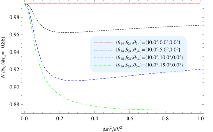
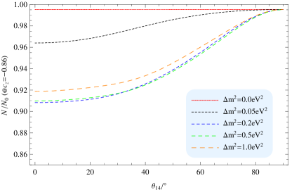
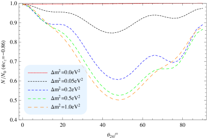
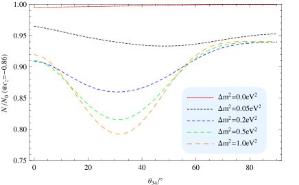
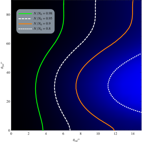
The main observable effect caused by a sterile neutrino in IceCube is tilting the zenith angle ($\cos\theta_{z}$) distribution of events, i.e. the smaller $c_{z}$ the more the event numbers are suppressed Esmaili and Smirnov (2013). The existence of sterile neutrinos causes disappearance for atmospheric neutrinos going through Earth. For a very small $|c_{z}|$ the corresponding oscillation baseline is very short hence neutrinos do not have enough time to oscillate before they arrive at the detector. So the survival probability is always very close to 1 if $c_{z}$ is small enough, no matter how large the mixing angles are. For a large $|c_{z}|$, neutrinos may have propagated over enough baseline to oscillate and thus the survival probability could be low. They may also experience several oscillatory periods before they arrive and the survival probability would be a value between the minimum and $1$, depending on energy and zenith angle. This qualitative analysis can be verified from Fig. 1, where $P$ is always close to 1 at $c_{z}\simeq 0$. For a large $|c_{z}|$, $P$ can be relatively small or still large (close to $1$), depending on $E$. Note that Eq. (31) is an integral over $E$ so only the average value (roughly) of $P$ is of importance. In this sense, we can say that the disappearance signal is stronger at larger $|c_{z}|$ and weaker at small $|c_{z}|$. Therefore, the sterile neutrino signal in the zenith angle distribution is mainly a tilting effect. To obtain a qualitative understanding of the sensitivity on sterile neutrino parameters, we plot in Fig. 2 for illustration $N/N_{0}$ at $c_{z}=-0.86$ for the various sterile neutrino parameters ($\Delta m^{2},\theta_{14},\theta_{24},\theta_{34}$), i.e. the ratio of events for the oscillated and unoscillated case at a large zenith angle. The more this quantity deviates from $1$, the more the zenith angle distribution tilts. The upper left $\Delta m^{2}$-plot shows that $N/N_{0}$ drops down quickly from $1$ when $\Delta m^{2}$ goes from $0$ to $0.1\,{\rm eV}^{2}$. This implies that the sensitivity of IceCube on sterile neutrinos depends on $\Delta m^{2}$ significantly at this range. The upper right $\theta_{14}$-plot shows that $N/N_{0}$ changes very little for $\theta_{14}\in[0^{\circ},20^{\circ}]$ which means IceCube is insensitive to small $\theta_{14}$ (note that large $\theta_{14}$ has been excluded by reactor neutrino experiments). There is almost no difference between $\theta_{14}=0^{\circ}$ and $10^{\circ}$ for IceCube. The angle $\theta_{24}$ is the most sensitive parameter as shown in the lower left $\theta_{24}$-plot. For (too) large $\theta_{24}$ such as $40^{\circ}$, $N/N_{0}$ could drop to $0.5$. For small $\theta_{24}$, we should include $\theta_{34}$ in the sensitivity analysis because the matter effect resonance is sensitive to the ratio $U_{\mu 4}/U_{\tau 4}=\tan\theta_{24}/\sin\theta_{34}$, see Eq. (26). Moreover, the important matter effect could decouple for large $\theta_{34}$, as we have discussed in Section III. We therefore plot $N/N_{0}$ in the $\theta_{24}-\theta_{34}$ plane in Fig. 3, where we can see that for $\theta_{34}=20^{\circ}$ even a small $\theta_{24}$ value ($8^{\circ}$) can make $N/N_{0}$ drop to $0.9$. Note that when $\theta_{34}$ is close to $90^{\circ}$ then as we have mentioned in the analytic discussion, $\nu_{\mu}$ ($\overline{\nu}_{\mu}$) neutrinos would oscillate as if they are in vacuum. So generally speaking, the signal of sterile neutrinos for $\theta_{34}=90^{\circ}$ is weaker than for other values.

Figure 4: Event numbers versus zenith angle $\cos\theta_{z}$ for several cases. The atmospheric neutrino flux is normalized by a factor of $1+a$, see Eq. (34). The data can be fitted very well without any sterile neutrino contribution.

$\log_{10}(\Delta m^{2}/{\rm eV}^{2})$

\begin{overpic}[width=170.71652pt]{fig/8plotsL-0} \put(10.0,85.0){$\theta_{34}=0^{\circ}$} \put(10.0,80.0){$\theta_{14}=10^{\circ}$} \end{overpic}\begin{overpic}[width=170.71652pt]{fig/8plotsR-0} \put(10.0,85.0){$\theta_{34}=0^{\circ}$} \put(10.0,80.0){$\theta_{14}=4^{\circ}$} \end{overpic}\begin{overpic}[width=170.71652pt]{fig/8plotsL-1} \put(10.0,85.0){$\theta_{34}=10^{\circ}$} \put(10.0,80.0){$\theta_{14}=10^{\circ}$} \end{overpic}\begin{overpic}[width=170.71652pt]{fig/8plotsR-1} \put(10.0,85.0){$\theta_{34}=10^{\circ}$} \put(10.0,80.0){$\theta_{14}=4^{\circ}$} \end{overpic}\begin{overpic}[width=170.71652pt]{fig/8plotsL-3} \put(10.0,15.0){$\theta_{34}=30^{\circ}$} \put(10.0,10.0){$\theta_{14}=10^{\circ}$} \end{overpic}\begin{overpic}[width=170.71652pt]{fig/8plotsR-3} \put(10.0,15.0){$\theta_{34}=30^{\circ}$} \put(10.0,10.0){$\theta_{14}=4^{\circ}$} \end{overpic}\begin{overpic}[width=170.71652pt]{fig/8plotsL-9} \put(10.0,85.0){$\theta_{34}=90^{\circ}$} \put(10.0,80.0){$\theta_{14}=10^{\circ}$} \end{overpic}\begin{overpic}[width=170.71652pt]{fig/8plotsR-9} \put(10.0,85.0){$\theta_{34}=90^{\circ}$} \put(10.0,80.0){$\theta_{14}=4^{\circ}$} \end{overpic}

$\log_{10}\sin^{2}2\theta_{24}$

Figure 5: Exclusion bounds for $(\Delta m^{2},\sin^{2}2\theta_{24})$. In these plots, $\theta_{34}$ is fixed at (from top to bottom) $0^{\circ}$, $10^{\circ}$, $30^{\circ}$ and $90^{\circ}$; $\theta_{14}$ at $10{}^{\circ}$ (left) or $4^{\circ}$ (right). Also shown are 99% C.L. fit results from the world’s appearance and disappearance data in purple (from Kopp et al. Kopp et al. (2013)), in yellow (from Giunti et al. Gariazzo et al. (2015)) and in the white contour (from Conrad et al. Conrad et al. (2013)). The blue contour line is the result of an appearance data only fit from Kopp et al. (2013).

IV $\chi^{2}$-fit and result

We perform now a numerical analysis of the IceCube-59 data from Ref. Aartsen et al. (2014), adopting a conventional $\chi^{2}$-function

$$\chi^{2}(\theta_{14},\theta_{24},\theta_{34},\Delta m^{2},a)=\frac{a^{2}}{\sigma_{a}^{2}}+\sum_{i=c_{z}\thinspace{\rm bins}}\frac{[(1+a)N_{{\rm th},i}-N_{{\rm ob},i}]^{2}}{\sigma_{{\rm stat},i}^{2}+\sigma_{{\rm sys},i}^{2}}\,,$$ (34)

where $N_{{\rm ob},i}$ is the observed event number in each bin with statistical uncertainty $\sigma_{{\rm stat},i}^{2}$ and $N_{{\rm th},i}$ is the predicted event number for each bin. Since the events number in each bin is large enough, we can simply take $\sigma_{{\rm stat},i}=\sqrt{N_{{\rm ob},i}}$. For the systematic uncertainty we take, according to ICR , $\sigma_{{\rm sys},i}=0.04N_{{\rm ob},i}$. The factor $1+a$ in front of $N_{{\rm th},i}$ is the normalization factor of the full flux with a large uncertainty, for instance $\sigma_{a}=15\%$ at $10^{2}$ GeV or $25\%$ at $10^{3}$ GeV (see Fig. 11 in Honda et al. (2007)). The major constraint on sterile neutrinos comes from the second term in Eq. (34). For minimization of the $\chi^{2}$-function, it is easy to compute the value of $a$ at the minimum analytically:

$$a_{{\rm min}}=\frac{\sum_{i}(N_{{\rm ob},i}-N_{{\rm th},i})N_{{\rm th},i}/d_{i}}{\sigma_{a}^{-2}+\sum_{i}N_{{\rm th},i}^{2}/d_{i}}\,.$$ (35)

Here $d_{i}\equiv\sigma_{{\rm stat},i}^{2}+\sigma_{{\rm sys},i}^{2}$. In practice, we will use Eq. (35) for the minimization of the $\chi^{2}$-function.

Let us first simply fix $\theta_{14}$ and $\theta_{34}$ to certain values so $\chi^{2}$ is a function of $\theta_{24},\thinspace\Delta m^{2}$ and $a$. The conventional treatment is then to replace $a$ in the $\chi^{2}$-function with $a_{{\rm min}}$ given by Eq. (35). After that, $\chi^{2}$ will be a function only of $\theta_{24}$ and $\Delta m^{2}$. We perform the $\chi^{2}$-fit for several cases. For instance, for $(\theta_{14},\theta_{34})=(10^{\circ},0^{\circ})$ we find the best-fit point is $\theta_{24}=8.3^{\circ}$, $\Delta m^{2}=0.014\,{\rm eV}^{2}$ with $\chi_{{\rm min}}^{2}=9.19$. 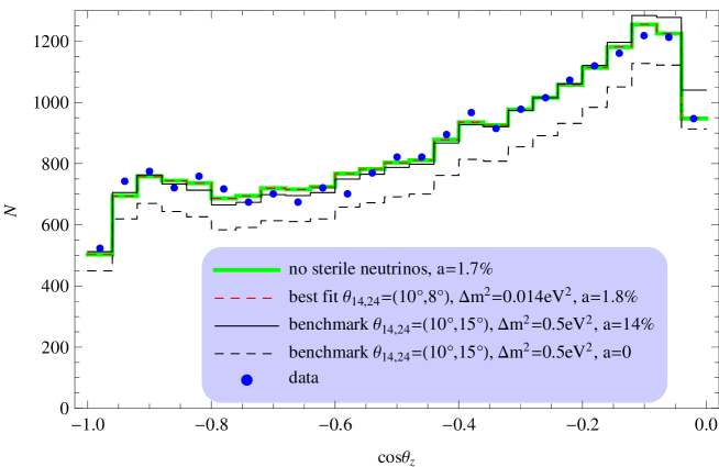This is no significant effect as for $\theta_{24}=0^{\circ}$ (i.e., no sterile neutrinos) $\chi^{2}=9.43$ is essentially an equivalently good fit to the data. In Fig. 4 we show the event distributions of some cases where we can see that the best-fit curve (red, dashed) almost overlaps with the green curve (no sterile neutrinos).

In Fig. 5 we plot the $90\%,95\%,99.73\%$ exclusion bounds (i.e. contours for $\chi^{2}-\chi_{{\rm min}}^{2}=4.61,5.99,11.83$) in the $\sin^{2}2\theta_{24}-\Delta m^{2}$ plane, for several cases. We also display for comparison the 99% C.L. regions of various global fit results on $\sin^{2}2\theta_{e\mu}$ from Refs. Kopp et al. (2013); Gariazzo et al. (2015); Conrad et al. (2013). Though that signal depends on $\sin^{2}2\theta_{\mu e}=\sin^{2}2\theta_{14}\sin^{2}\theta_{24}$ and $\Delta m^{2}$, we can use the fixed value $\theta_{14}=10{}^{\circ}$ (or $4^{\circ}$) to convert the LSND constraint from $\sin^{2}2\theta_{\mu e}$ to $\sin^{2}2\theta_{24}$. The Super-Kamiokande result on $|U_{\mu 4}|^{2}$ is also given Abe et al. (2015).

\begin{overpic}[width=170.71652pt]{fig/m2s24plotsL} \put(20.0,85.0){$\theta_{14}=10^{\circ}$} \end{overpic}

\begin{overpic}[width=170.71652pt]{fig/m2s24plotsR} \put(20.0,85.0){$\theta_{14}=4^{\circ}$} \end{overpic}

Figure 6: Exclusion bounds for $(\Delta m^{2},\sin^{2}2\theta_{24})$ after marginalizing over $\theta_{34}$; $\theta_{14}$ is fixed to $10{}^{\circ}$ (left) or $4^{\circ}$ (right). Also shown are 99% C.L. fit results from the world’s appearance and disappearance data in purple (from Kopp et al. Kopp et al. (2013)), in yellow (from Giunti et al. Gariazzo et al. (2015)) and in the white contour (from Conrad et al. Conrad et al. (2013)). The blue contour line is the result of an appearance data only fit from Kopp et al. (2013).

We see from Fig. 5 that the value of $\theta_{34}$ is very important. As one increases $\theta_{34}$ from zero, the constraint becomes stronger until $\theta_{34}$ is large enough. After that, the constraint becomes weaker when $\theta_{34}$ is increased. This can be understood via Fig. 2, where in the bottom right panel we can see the event number generally drops down (which implies the disappearance of neutrinos) when $\theta_{34}$ is increased from $0^{\circ}$. The event number reaches its minimum at about $30^{\circ}$ and then increases because for $\theta_{34}=90^{\circ}$, as we have discussed, the signal of sterile neutrinos is weak since there is no matter effect enhancement. $\theta_{14}$, however, has little influence on the IceCube result for $\Delta m^{2}$ and $\sin^{2}2\theta_{24}$. But the angle is important to compare the outcome to the short baseline appearance data. Note that with $\theta_{14}=0$ there would be no short baseline appearance oscillations, see Eq. (25). The larger $\theta_{14}$, the smaller the value of $\theta_{24}$ necessary to generate the same value of $\sin^{2}\theta_{\mu e}$, hence it becomes more difficult for IceCube to rule it out. Marginalizing over $\theta_{34}$ results in Fig. 6. We see that for $\theta_{14}=10^{\circ}$ the appearance signal is partially compatible within $90\%$, but ruled out at $99.73\%$ if $\theta_{14}=4^{\circ}$. Regarding the appearance plus disappearance data, strong dependence on the fit result exists. For $\theta_{14}=10^{\circ}$, the signal from Gariazzo et al. (2015) is fully consistent with IceCube-59 at $90\%$, whereas the full regime from Kopp et al. (2013) and a part of the regime from from Conrad et al. (2013) are excluded at $90\%$. At $\theta_{14}=4^{\circ}$, the signal from Gariazzo et al. (2015) still cannot be ruled out at about $90\%$, whereas the full regime from Kopp et al. (2013) and the one from Conrad et al. (2013) are ruled out at $95\%$. Such strong dependence on fit results and parameters not appearing in IceCube expressions will also be present in fits of IceCube-86 data, not yet available, and should be taken into account when interpreting the results.

V Conclusion

We have performed a $\chi^{2}$-fit to IceCube-59 data in order to constrain sterile neutrino mixing parameters. Special emphasis was put on the question on how muon neutrino disappearance compares to the muon neutrino disappearance in short baseline experiments and other sterile neutrino results. We have stressed the different dependence on the three relevant mixing angles and the important role of the very weakly constrained angle $\theta_{34}$, which governs the strength of the matter resonance, and is often set to zero in analyses. The value of $\theta_{14}$ is also crucial. Fixing this angle implies via the short baseline appearance results the value of $\theta_{24}$, on which the analysis of IceCube data is most sensitive to. It was demonstrated that only part of the global parameter space is currently constrained by IceCube, though of course important complementary information is provided. Moreover, there is dependence on which fit result one compares the data to.

The comparison of the various oscillation channels relies on several assumptions, in particular the presence of only one sterile neutrino. In this framework we assume unitarity of the $4\times 4$ mixing matrix, and the absence of additional interactions that sterile neutrinos could be sensitive to. As even with these assumptions no final solution to the short baseline disappearance and other problems can be given, it shows that several dedicated oscillation experiments are required to fully settle the issue.