Generalizing Pooling Functions in Convolutional Neural Networks:
Mixed, Gated, and Tree
Chen-Yu Lee Patrick W. Gallagher Zhuowen Tu
UCSD ECE UCSD Cognitive Science UCSD Cognitive Science
chl260@ucsd.edu patrick.w.gallagher@gmail.com ztu@ucsd.edu
Abstract
We seek to improve deep neural networks by generalizing the pooling operations that play a central role in current architectures. We pursue a careful exploration of approaches to allow pooling to learn and to adapt to complex and variable patterns. The two primary directions lie in (1) learning a pooling function via (two strategies of) combining of max and average pooling, and (2) learning a pooling function in the form of a tree-structured fusion of pooling filters that are themselves learned. In our experiments every generalized pooling operation we explore improves performance when used in place of average or max pooling. We experimentally demonstrate that the proposed pooling operations provide a boost in invariance properties relative to conventional pooling and set the state of the art on several widely adopted benchmark datasets; they are also easy to implement, and can be applied within various deep neural network architectures. These benefits come with only a light increase in computational overhead during training and a very modest increase in the number of model parameters.
1 Introduction
The recent resurgence of neurally-inspired systems such as deep belief nets (DBN) [10], convolutional neural networks (CNNs) [18], and the sum-and-max infrastructure [32] has derived significant benefit from building more sophisticated network structures [38, 33] and from bringing learning to non-linear activations [6, 24]. The pooling operation has also played a central role, contributing to invariance to data variation and perturbation. However, pooling operations have been little revised beyond the current primary options of average, max, and stochastic pooling [3, 40]; this despite indications that e.g. choosing from more than just one type of pooling operation can benefit performance [31].
In this paper, we desire to bring learning and “responsiveness” (i.e., to characteristics of the region being pooled) into the pooling operation. Various approaches are possible, but here we pursue two in particular. In the first approach, we consider combining typical pooling operations (specifically, max pooling and average pooling); within this approach we further investigate two strategies by which to combine these operations. One of the strategies is “unresponsive”; for reasons discussed later, we call this strategy mixed max-average pooling. The other strategy is “responsive”; we call this strategy gated max-average pooling, where the ability to be responsive is provided by a “gate” in analogy to the usage of gates elsewhere in deep learning.
Another natural generalization of pooling operations is to allow the pooling operations that are being combined to themselves be learned. Hence in the second approach, we learn to combine pooling filters that are themselves learned. Specifically, the learning is performed within a binary tree (with number of levels that is pre-specified rather than “grown” as in traditional decision trees) in which each leaf is associated with a learned pooling filter. As we consider internal nodes of the tree, each parent node is associated with an output value that is the mixture of the child node output values, until we finally reach the root node. The root node corresponds to the overall output produced by the tree. We refer to this strategy as tree pooling. Tree pooling is intended (1) to learn pooling filters directly from the data; (2) to learn how to combine leaf node pooling filters in a differentiable fashion; (3) to bring together these other characteristics within a hierarchical tree structure.
When the mixing of the node outputs is allowed to be “responsive”, the resulting tree pooling operation becomes an integrated method for learning pooling filters and combinations of those filters that are able to display a range of different behaviors depending on the characteristics of the region being pooled.
We pursue experimental validation and find that: In the architectures we investigate, replacing standard pooling operations with any of our proposed generalized pooling methods boosts performance on each of the standard benchmark datasets, as well as on the larger and more complex ImageNet dataset. We attain state-of-the-art results on MNIST, CIFAR10 (with and without data augmentation), and SVHN. Our proposed pooling operations can be used as drop-in replacements for standard pooling operations in various current architectures and can be used in tandem with other performance-boosting approaches such as learning activation functions, training with data augmentation, or modifying other aspects of network architecture — we confirm improvements when used in a DSN-style architecture, as well as in AlexNet and GoogLeNet. Our proposed pooling operations are also simple to implement, computationally undemanding (ranging from to additional overhead in timing experiments), differentiable, and use only a modest number of additional parameters.
2 Related Work
In the current deep learning literature, popular pooling functions include max, average, and stochastic pooling [3, 2, 40]. A recent effort using more complex pooling operations, spatial pyramid pooling [9], is mainly designed to deal with images of varying size, rather than delving in to different pooling functions or incorporating learning. Learning pooling functions is analogous to receptive field learning [8, 11, 5, 15]. However methods like [15] lead to a more difficult learning procedure that in turn leads to a less competitive result, e.g. an error rate of on unaugmented CIFAR10.
Since our tree pooling approach involves a tree structure in its learning, we observe an analogy to “logic-type” approaches such as decision trees [27] or “logical operators” [25]. Such approaches have played a central role in artificial intelligence for applications that require “discrete” reasoning, and are often intuitively appealing. Unfortunately, despite the appeal of such logic-type approaches, there is a disconnect between the functioning of decision trees and the functioning of CNNs — the output of a standard decision tree is non-continuous with respect to its input (and thus nondifferentiable). This means that a standard decision tree is not able to be used in CNNs, whose learning process is performed by back propagation using gradients of differentiable functions. Part of what allows us to pursue our approaches is that we ensure the resulting pooling operation is differentiable and thus usable within network backpropagation.
A recent work, referred to as auto-encoder trees [13], also pays attention to a differentiable use of tree structures in deep learning, but is distinct from our method as it focuses on learning encoding and decoding methods (rather than pooling methods) using a “soft” decision tree for a generative model. In the supervised setting, [4] incorporates multilayer perceptrons within decision trees, but simply uses trained perceptrons as splitting nodes in a decision forest; not only does this result in training processes that are separate (and thus more difficult to train than an integrated training process), this training process does not involve the learning of any pooling filters.
3 Generalizing Pooling Operations
A typical convolutional neural network is structured as a series of convolutional layers and pooling layers. Each convolutional layer is intended to produce representations (in the form of activation values) that reflect aspects of local spatial structures, and to consider multiple channels when doing so. More specifically, a convolution layer computes “feature response maps” that involve multiple channels within some localized spatial region. On the other hand, a pooling layer is restricted to act within just one channel at a time, “condensing” the activation values in each spatially-local region in the currently considered channel. An early reference related to pooling operations (although not explicitly using the term “pooling”) can be found in [11]. In modern visual recognition systems, pooling operations play a role in producing “downstream” representations that are more robust to the effects of variations in data while still preserving important motifs. The specific choices of average pooling [18, 19] and max pooling [28] have been widely used in many CNN-like architectures; [3] includes a theoretical analysis (albeit one based on assumptions that do not hold here).
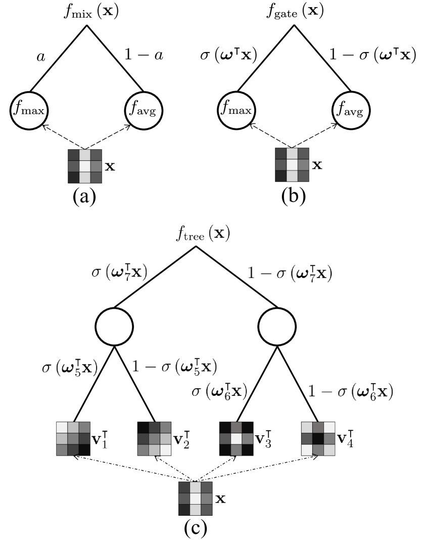
Our goal is to bring learning and “responsiveness” into the pooling operation. We focus on two approaches in particular. In the first approach, we begin with the (conventional, non-learned) pooling operations of max pooling and average pooling and learn to combine them. Within this approach, we further consider two strategies by which to combine these fixed pooling operations. One of these strategies is “unresponsive” to the characteristics of the region being pooled; the learning process in this strategy will result in an effective pooling operation that is some specific, unchanging “mixture” of max and average. To emphasize this unchanging mixture, we refer to this strategy as mixed max-average pooling.
The other strategy is “responsive” to the characteristics of the region being pooled; the learning process in this strategy results in a “gating mask”. This learned gating mask is then used to determine a “responsive” mix of max pooling and average pooling; specifically, the value of the inner product between the gating mask and the current region being pooled is fed through a sigmoid, the output of which is used as the mixing proportion between max and average. To emphasize the role of the gating mask in determining the “responsive” mixing proportion, we refer to this strategy as gated max-average pooling.
Both the mixed strategy and the gated strategy involve combinations of fixed pooling operations; a complementary generalization to these strategies is to learn the pooling operations themselves. From this, we are in turn led to consider learning pooling operations and also learning to combine those pooling operations. Since these combinations can be considered within the context of a binary tree structure, we refer to this approach as tree pooling. We pursue further details in the following sections.
3.1 Combining max and average pooling functions
3.1.1 “Mixed” max-average pooling
The conventional pooling operation is fixed to be either a simple average or a maximum operation , where the vector contains the activation values from a local pooling region of pixels (typical pooling region dimensions are or ) in an image or a channel.
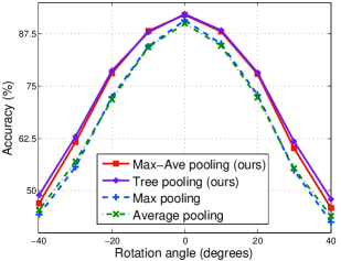
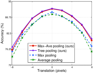
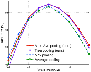
At present, max pooling is often used as the default in CNNs. We touch on the relative performance of max pooling and, e.g., average pooling as part of a collection of exploratory experiments to test the invariance properties of pooling functions under common image transformations (including rotation, translation, and scaling); see Figure 2. The results indicate that, on the evaluation dataset, there are regimes in which either max pooling or average pooling demonstrates better performance than the other (although we observe that both of these choices are outperformed by our proposed pooling operations). In the light of observation that neither max pooling nor average pooling dominates the other, a first natural generalization is the strategy we call “mixed” max-average pooling, in which we learn specific mixing proportion parameters from the data. When learning such mixing proportion parameters one has several options (listed in order of increasing number of parameters): learning one mixing proportion parameter (a) per net, (b) per layer, (c) per layer/region being pooled (but used for all channels across that region), (d) per layer/channel (but used for all regions in each channel) (e) per layer/region/channel combination.
The form for each “mixed” pooling operation (written here for the “one per layer” option; the expression for other options differs only in the subscript of the mixing proportion ) is:
| (1) |
where is a scalar mixing proportion specifying the specific combination of max and average; the subscript is used to indicate that this equation is for the “one per layer” option. Once the output loss function is defined, we can automatically learn each mixing proportion (where we now suppress any subscript specifying which of the options we choose). Vanilla backpropagation for this learning is given by
| (2) |
where is the error backpropagated from the following layer. Since pooling operations are typically placed in the midst of a deep neural network, we also need to compute the error signal to be propagated back to the previous layer:
| (3) | ||||
| (4) |
where denotes the indicator function. In the experiment section, we report results for the “one parameter per pooling layer” option; the network for this experiment has 2 pooling layers and so has 2 more parameters than a network using standard pooling operations. We found that even this simple option yielded a surprisingly large performance boost. We also obtain results for a simple 50/50 mix of max and average, as well as for the option with the largest number of parameters: one parameter for each combination of layer/channel/region, or parameters for each “mixed” pooling layer using this option (where is the number of channels being pooled by the pooling layer, and the number of spatial regions being pooled in each channel is ). We observe that the increase in the number of parameters is not met with a corresponding boost in performance, and so we pursue the “one per layer” option.
3.1.2 “Gated” max-average pooling
In the previous section we considered a strategy that we referred to as “mixed” max-average pooling; in that strategy we learned a mixing proportion to be used in combining max pooling and average pooling. As mentioned earlier, once learned, each mixing proportion remains fixed — it is “nonresponsive” insofar as it remains the same no matter what characteristics are present in the region being pooled. We now consider a “responsive” strategy that we call “gated” max-average pooling. In this strategy, rather than directly learning a mixing proportion that will be fixed after learning, we instead learn a “gating mask” (with spatial dimensions matching that of the regions being pooled). The scalar result of the inner product between the gating mask and the region being pooled is fed through a sigmoid to produce the value that we use as the mixing proportion. This strategy means that the actual mixing proportion can vary during use depending on characteristics present in the region being pooled. To be more specific, suppose we use to denote the values in the region being pooled and to denote the values in a “gating mask”. The “responsive” mixing proportion is then given by , where is a sigmoid function.
Analogously to the strategy of learning mixing proportion parameter, when learning gating masks one has several options (listed in order of increasing number of parameters): learning one gating mask (a) per net, (b) per layer, (c) per layer/region being pooled (but used for all channels across that region), (d) per layer/channel (but used for all regions in each channel) (e) per layer/region/channel combination. We suppress the subscript denoting the specific option, since the equations are otherwise identical for each option.
The resulting pooling operation for this “gated” max-average pooling is:
| (5) |
We can compute the gradient with respect to the internal “gating mask” using the same procedure considered previously, yielding
| (6) | ||||
| (7) |
and
| (8) | ||||
| (9) | ||||
In a head-to-head parameter count, every single mixing proportion parameter in the “mixed” max-average pooling strategy corresponds to a gating mask in the “gated” strategy (assuming they use the same parameter count option). To take a specific example, suppose that we consider a network with 2 pooling layers and pooling regions that are . If we use the “mixed” strategy and the per-layer option, we would have a total of extra parameters relative to standard pooling. If we use the “gated” strategy and the per-layer option, we would have a total of extra parameters, where is the number of parameters in each gating mask. The “mixed” strategy detailed immediately above uses fewer parameters and is “nonresponsive”; the “gated” strategy involves more parameters and is “responsive”. In our experiments, we find that “mixed” (with one mix per pooling layer) is outperformed by “gated” with one gate per pooling layer. Interestingly, an parameter “gated” network with only one gate per pooling layer also outperforms a “mixed” option with far more parameters ( with one mix per layer/channel/region) — except on the relatively large SVHN dataset. We touch on this below; Section 5 contains details.
3.1.3 Quick comparison: mixed and gated pooling
The results in Table 1 indicate the benefit of learning pooling operations over not learning. Within learned pooling operations, we see that when the number of parameters in the mixed strategy is increased, performance improves; however, parameter count is not the entire story. We see that the “responsive” gated max-avg strategy consistently yields better performance (using 18 extra parameters) than is achieved with the 40k extra parameters in the 1 per layer/rg/ch “non-responsive” mixed max-avg strategy. The relatively larger SVHN dataset provides the sole exception (SVHN has 600k training images versus 50k for MNIST, CIFAR10, and CIFAR100) — we found baseline 1.91%, 50/50 mix 1.84%, mixed (1 per lyr) 1.76%, mixed (1 per lyr/ch/rg) 1.64%, and gated (1 per lyr) 1.74%.
| Method | MNIST | CIFAR10 | CIFAR10+ | CIFAR100 |
|---|---|---|---|---|
| Baseline | 0.39 | 9.10 | 7.32 | 34.21 |
| w/ Stochastic no learning | 0.38 0.04 | 8.50 0.05 | 7.30 0.07 | 33.48 0.27 |
| w/ 50/50 mix no learning | 0.34 0.012 | 8.11 0.10 | 6.78 0.17 | 33.53 0.16 |
| w/ Mixed 1 per pool layer 2 extra params | 0.33 0.018 | 8.09 0.19 | 6.62 0.21 | 33.51 0.11 |
| w/ Mixed 1 per layer/ch/rg 40k extra params | 0.30 0.012 | 8.05 0.16 | 6.58 0.30 | 33.35 0.19 |
| w/ Gated 1 per pool layer 18 extra params | 0.29 0.016 | 7.90 0.07 | 6.36 0.28 | 33.22 0.16 |
3.2 Tree pooling
The strategies described above each involve combinations of fixed pooling operations; another natural generalization of pooling operations is to allow the pooling operations that are being combined to themselves be learned. These pooling layers remain distinct from convolution layers since pooling is performed separately within each channel; this channel isolation also means that even the option that introduces the largest number of parameters still introduces far fewer parameters than a convolution layer would introduce. The most basic version of this approach would not involve combining learned pooling operations, but simply learning pooling operations in the form of the values in “pooling filters”. One step further brings us to what we refer to as tree pooling, in which we learn pooling filters and also learn to responsively combine those learned filters.
Both aspects of this learning are performed within a binary tree (with number of levels that is pre-specified rather than “grown” as in traditional decision trees) in which each leaf is associated with a pooling filter learned during training. As we consider internal nodes of the tree, each parent node is associated with an output value that is the mixture of the child node output values, until we finally reach the root node. The root node corresponds to the overall output produced by the tree and each of the mixtures (by which child outputs are “fused” into a parent output) is responsively learned. Tree pooling is intended (1) to learn pooling filters directly from the data; (2) to learn how to “mix” leaf node pooling filters in a differentiable fashion; (3) to bring together these other characteristics within a hierarchical tree structure.
Each leaf node in our tree is associated with a “pooling filter” that will be learned; for a node with index , we denote the pooling filter by . If we had a “degenerate tree” consisting of only a single (leaf) node, pooling a region would result in the scalar value . For (internal) nodes (at which two child values are combined into a single parent value), we proceed in a fashion analogous to the case of gated max-average pooling, with learned “gating masks” denoted (for an internal node ) by . The “pooling result” at any arbitrary node is thus
| (10) |
The overall pooling operation would thus be the result of evaluating . The appeal of this tree pooling approach would be limited if one could not train the proposed layer in a fashion that was integrated within the network as a whole. This would be the case if we attempted to directly use a traditional decision tree, since its output presents points of discontinuity with respect to its inputs. The reason for the discontinuity (with respect to input) of traditional decision tree output is that a decision tree makes “hard” decisions; in the terminology we have used above, a “hard” decision node corresponds to a mixing proportion that can only take on the value or . The consequence is that this type of “hard” function is not differentiable (nor even continuous with respect to its inputs), and this in turn interferes with any ability to use it in iterative parameter updates during backpropagation. This motivates us to instead use the internal node sigmoid “gate” function so that the tree pooling function as a whole will be differentiable with respect to its parameters and its inputs.
For the specific case of a “2 level” tree (with leaf nodes “1” and “2” and internal node “3”) pooling function , we can use the chain rule to compute the gradients with respect to the leaf node pooling filters and the internal node gating mask :
| (11) |
| (12) |
| (13) |
The error signal to be propagated back to the previous layer is
| (14) | ||||
| (15) | ||||
3.2.1 Quick comparison: tree pooling
Table 2 collects results related to tree pooling. We observe that on all datasets but the comparatively simple MNIST, adding a level to the tree pooling operation improves performance. However, even further benefit is obtained from the use of tree pooling in the first pooling layer and gated max-avg in the second.
| Method | MNIST | CIFAR10 | CIFAR10+ | CIFAR100 | SVHN |
|---|---|---|---|---|---|
| Our baseline | 0.39 | 9.10 | 7.32 | 34.21 | 1.91 |
| Tree 2 level; 1 per pool layer | 0.35 | 8.25 | 6.88 | 33.53 | 1.80 |
| Tree 3 level; 1 per pool layer | 0.37 | 8.22 | 6.67 | 33.13 | 1.70 |
| Tree+Max-Avg 1 per pool layer | 0.31 | 7.62 | 6.05 | 32.37 | 1.69 |
Comparison with making the network deeper using conv layers To further investigate whether simply “adding depth” to our baseline network gives a performance boost comparable to that observed for our proposed pooling operations, we report in Table 3 below some additional experiments on CIFAR10 (error rate in percent; no data augmentation). If we count depth by counting any layer with learned parameters as an extra layer of depth (even if there is only 1 parameter), the number of parameter layers in a baseline network with 2 additional standard convolution layers matches the number of parameter layers in our best performing net (although the convolution layers contain many more parameters).
Our method requires only extra parameters and obtains state-of-the-art error. On the other hand, making networks deeper with conv layers adds many more parameters but yields test error that does not drop below in the configuration explored. Since we follow each additional conv layer with a ReLU, these networks correspond to increasing nonlinearity as well as adding depth and adding (many) parameters. These experiments indicate that the performance of our proposed pooling is not accounted for as a simple effect of the addition of depth/parameters/nonlinearity.
| Method | % Error | Extra parameters |
|---|---|---|
| Baseline | 9.10 | 0 |
| w/ 1 extra conv layer (+ReLU) | 9.08 | 0.6M |
| w/ 2 extra conv layers (+ReLU) | 9.17 | 1.2M |
| w/ Tree+(gated) Max-Avg | 7.62 | 72 |
Comparison with alternative pooling layers To see whether we might find similar performance boosts by replacing the max pooling in the baseline network configuration with alternative pooling operations such as stochastic pooling, “pooling” using a stride 2 convolution layer as pooling (cf All-CNN), or a simple fixed 50/50 proportion in max-avg pooling, we performed another set of experiments on unaugmented CIFAR10. From the baseline error rate of 9.10%, replacing each of the 2 max pooling layers with stacked stride 2 conv:ReLU (as in [34]) lowers the error to 8.77%, but adds 0.5M extra parameters. Using stochastic pooling [40] adds computational overhead but no parameters and results in 8.50% error. A simple 50/50 mix of max and average is computationally light and yields 8.07% error with no additional parameters. Finally, our tree+gated max-avg configuration adds 72 parameters and achieves a state-of-the-art 7.62% error.
4 Quick Performance Overview
For ease of discussion, we collect here observations from subsequent experiments with a view to highlighting aspects that shed light on the performance characteristics of our proposed pooling functions.
First, as seen in the experiment shown in Figure 2 replacing standard pooling operations with either gated max-avg or (2 level) tree pooling (each using the “one per layer” option) yielded a boost (relative to max or avg pooling) in CIFAR10 test accuracy as the test images underwent three different kinds of transformations. This boost was observed across the entire range of transformation amounts for each of the transformations (with the exception of extreme downscaling). We already observe improved robustness in this initial experiment and intend to investigate more instances of our proposed pooling operations as time permits.
Second, the performance that we attain in the experiments reported in Figure 2, Table 1, Table 2, Table 4, and Table 5 is achieved with very modest additional numbers of parameters — e.g. on CIFAR10, our best performance (obtained with the tree+gated max-avg configuration) only uses an additional parameters (above the 1.8M of our baseline network) and yet reduces test error from to ; see the CIFAR10 Section for details. In our AlexNet experiment, replacing the maxpool layers with our proposed pooling operations gave a relative reduction in test error (top-5, single-view) with only 45 additional parameters (above the 50M of standard AlexNet); see the ImageNet 2012 Section for details. We also investigate the additional time incurred when using our proposed pooling operations; in the experiments reported in the Timing section, this overhead ranges from to .
Testing invariance properties Before going to the overall classification results, we investigate the invariance properties of networks utilizing either standard pooling operations (max and average) or two instances of our proposed pooling operations (gated max-avg and 2 level tree, each using the “1 per pool layer” option) that we find to yield best performance (see Sec. 5 for architecture details used across each network). We begin by training four different networks on the CIFAR10 training set, one for each of the four pooling operations selected for consideration; training details are found in Sec. 5. We seek to determine the respective invariance properties of these networks by evaluating their accuracy on various transformed versions of the CIFAR10 test set. Figure 2 illustrates the test accuracy attained in the presence of image rotation, (vertical) translation, and scaling of the CIFAR10 test set.
Timing In order to evaluate how much additional time is incurred by the use of our proposed learned pooling operations, we measured the average forward+backward time per CIFAR10 image. In each case, the one per layer option is used. We find that the additional computation time incurred ranges from to . More specifically, the baseline network took 3.90 ms; baseline with mixed max-avg took 4.10 ms; baseline with gated max-avg took 4.16 ms; baseline with 2 level tree pooling took 4.25 ms; finally, baseline with tree+gated max-avg took 4.46 ms.
5 Experiments
We evaluate the proposed max-average pooling and tree pooling approaches on five standard benchmark datasets: MNIST [20], CIFAR10 [16], CIFAR100 [16], SVHN [26] and ImageNet [30]. To control for the effect of differences in data or data preparation, we match our data and data preparation to that used in [21]. Please refer to [21] for the detailed description.
We now describe the basic network architecture and then will specify the various hyperparameter choices. The basic experiment architecture contains six standard convolutional layers (named conv1 to conv6) and three mlpconv layers (named mlpconv1 to mlpconv3) [24], placed after conv2, conv4, and conv6, respectively. We chose the number of channels at each layer to be analogous to the choices in [24, 21]; the specific numbers are provided in the sections for each dataset. We follow every one of these conv-type layers with ReLU activation functions. One final mlpconv layer (mlpconv4) is used to reduce the dimension of the last layer to match the total number of classes for each different dataset, as in [24]. The overall model has parameter count analogous to [24, 21]. The proposed max-average pooling and tree pooling layers with pooling regions are used after mlpconv1 and mlpconv2 layers 111There is one exception: on the very small images of the MNIST dataset, the second pooling layer uses pooling regions.. We provide a detailed listing of the network configurations in Table A1 in the Supplementary Materials.
Moving on to the hyperparameter settings, dropout with rate is used after each pooling layer. We also use hidden layer supervision to ease the training process as in [21]. The learning rate is decreased whenever the validation error stops decreasing; we use the schedule for all experiments. The momentum of and weight decay of are fixed for all datasets as another regularizer besides dropout. All the initial pooling filters and pooling masks have values sampled from a Gaussian distribution with zero mean and standard deviation . We use these hyperparameter settings for all experiments reported in Tables 1, 2, and 3. No model averaging is done at test time.
5.1 Classification results
Tables 1 and 2 show our overall experimental results. Our baseline is a network trained with conventional max pooling. Mixed refers to the same network but with a max-avg pooling strategy in both the first and second pooling layers (both using the mixed strategy); Gated has a corresponding meaning. Tree (with specific number of levels noted below) refers to the same again, but with our tree pooling in the first pooling layer only; we do not see further improvement when tree pooling is used for both pooling layers. This observation motivated us to consider following a tree pooling layer with a gated max-avg pooling layer: Tree+Max-Average refers to a network configuration with (2 level) tree pooling for the first pooling layer and gated max-average pooling for the second pooling layer. All results are produced from the same network structure and hyperparameter settings — the only difference is in the choice of pooling function. See Table A1 for details.
MNIST Our MNIST model has channels for conv1 to conv6 and channels for mlpconv1 to mlpconv3, respectively. Our only preprocessing is mean subtraction. Tables 4,1, and 2 show previous best results and those for our proposed pooling methods.
CIFAR10 Our CIFAR10 model has channels for conv1 to conv6 and channels for mlpconv1 to mlpconv3, respectively. We also performed an experiment in which we learned a single pooling filter without the tree structure (i.e., a singleton leaf node containing parameters; one such singleton leaf node per pooling layer) and obtained improvement over the baseline model. Our results indicate that performance improves when the pooling filter is learned, and further improves when we also learn how to combine learned pooling filters.
The All-CNN method in [34] uses convolutional layers in place of pooling layers in a CNN-type network architecture. However, a standard convolutional layer requires many more parameters than a gated max-average pooling layer (only parameters for a pooling region kernel size in the 1 per pooling layer option) or a tree-pooling layer ( parameters for a 2 level tree and pooling region kernel size, again in the 1 per pooling layer option). The pooling operations in our tree+max-avg network configuration use parameters for the (first, 3 level) tree-pooling layer — 4 leaf nodes and 3 internal nodes — and parameters in the gating mask used for the (second) gated max-average pooling layer, while the best result in [34] contains a total of nearly parameters in layers performing “pooling like” operations; the relative CIFAR10 accuracies are (ours) and (All-CNN).
For the data augmentation experiment, we followed the standard data augmentation procedure [24, 21, 34]. When training with augmented data, we observe the same trends seen in the “no data augmentation” experiments. We note that [7] reports a error rate with extensive data augmentation (including translations, rotations, reflections, stretching, and shearing operations) in a much wider and deeper million parameter network — times more than are in our networks.
| Method | MNIST | CIFAR10 | CIFAR10+ | CIFAR100 | SVHN |
|---|---|---|---|---|---|
| CNN [14] | 0.53 | - | - | - | - |
| Stoch. Pooling [40] | 0.47 | 15.13 | - | 42.51 | 2.80 |
| Maxout Networks [6] | 0.45 | 11.68 | 9.38 | 38.57 | 2.47 |
| Prob. Maxout [35] | - | 11.35 | 9.39 | 38.14 | 2.39 |
| Tree Priors [36] | - | - | - | 36.85 | - |
| DropConnect [22] | 0.57 | 9.41 | 9.32 | - | 1.94 |
| FitNet [29] | 0.51 | - | 8.39 | 35.04 | 2.42 |
| NiN [24] | 0.47 | 10.41 | 8.81 | 35.68 | 2.35 |
| DSN [21] | 0.39 | 9.69 | 7.97 | 34.57 | 1.92 |
| NiN + LA units [1] | - | 9.59 | 7.51 | 34.40 | - |
| dasNet [37] | - | 9.22 | - | 33.78 | - |
| All-CNN [34] | - | 9.08 | 7.25 | 33.71 | - |
| R-CNN [23] | 0.31 | 8.69 | 7.09 | 31.75 | 1.77 |
| Our baseline | 0.39 | 9.10 | 7.32 | 34.21 | 1.91 |
| Our Tree+Max-Avg | 0.31 | 7.62 | 6.05 | 32.37 | 1.69 |
CIFAR100 Our CIFAR100 model has channels for all convolutional layers and channels for mlpconv1 to mlpconv3, respectively.
Street view house numbers Our SVHN model has channels for conv1 to conv6 and channels for mlpconv1 to mlpconv3, respectively. In terms of amount of data, SVHN has a larger training data set (600k versus the 50k of most of the other benchmark datasets). The much larger amount of training data motivated us to explore what performance we might observe if we pursued the one per layer/channel/region option, which even for the simple mixed max-avg strategy results in a huge increase in total the number of parameters to learn in our proposed pooling layers: specifically, from a total of 2 in the mixed max-avg strategy, 1 parameter per pooling layer option, we increase to 40,960.
Using this one per layer/channel/region option for the mixed max-avg strategy, we observe test error (in ) of 0.30 on MNIST, 8.02 on CIFAR10, 6.61 on CIFAR10+, 33.27 on CIFAR100, and 1.64 on SVHN. Interestingly, for MNIST, CIFAR10+, and CIFAR100 this mixed max-avg (1 per layer/channel/region) performance is between mixed max-avg (1 per layer) and gated max-avg (1 per layer); on CIFAR10 mixed max-avg (1 per layer/channel/region) is worse than either of the 1 per layer max-avg strategies. The SVHN result using mixed max-avg (1 per layer/channel/region) sets a new state of the art.
ImageNet 2012 In this experiment we do not directly compete with the best performing result in the challenge (since the winning methods [38] involve many additional aspects beyond pooling operations), but rather to provide an illustrative comparison of the relative benefit of the proposed pooling methods versus conventional max pooling on this dataset. We use the same network structure and parameter setup as in [17] (no hidden layer supervision) but simply replace the first max pooling with the (proposed 2 level) tree pooling (2 leaf nodes and 1 internal node for parameters) and replace the second and third max pooling with gated max-average pooling (2 gating masks for parameters). Relative to the original AlexNet, this adds more parameters (over the 50M in the original) and achieves relative error reduction of (for top-5, single-view) and (for top-5, multi-view). Our GoogLeNet configuration uses 4 gated max-avg pooling layers, for a total of 36 extra parameters over the 6.8 million in standard GoogLeNet. Table 5 shows a direct comparison (in each case we use single net predictions rather than ensemble).
| Method | top-1 s-view | top-5 s-view | top-1 m-view | top-5 m-view |
|---|---|---|---|---|
| AlexNet [17] | 43.1 | 19.9 | 40.7 | 18.2 |
| AlexNet w/ ours | 41.4 | 18.7 | 39.3 | 17.3 |
| GoogLeNet [38] | - | 10.07 | - | 9.15 |
| GoogLeNet w/ BN | 28.68 | 9.53 | 27.81 | 9.09 |
| GoogLeNet w/ BN + ours | 28.02 | 9.16 | 27.60 | 8.93 |
6 Observations from Experiments
In each experiment, using any of our proposed pooling operations boosted performance. A fixed network configuration using the proposed tree+max-avg pooling (1 per pool layer option) yields state-of-the-art performance on MNIST, CIFAR10 (with and without data augmentation), and SVHN. We observed boosts in tandem with data augmentation, multi-view predictions, batch normalization, and several different architectures — NiN-style, DSN-style, the 50M parameter AlexNet, and the 22-layer GoogLeNet.
Acknowledgment This work is supported by NSF awards IIS-1216528 (IIS-1360566) and IIS-0844566(IIS-1360568).
References
- [1] F. Agostinelli, M. Hoffman, P. Sadowski, and P. Baldi. Learning activation functions to improve deep neural networks. In ICLR, 2015.
- [2] Y. Boureau, N. Le Roux, F. Bach, J. Ponce, and Y. LeCun. Ask the locals: multi-way local pooling for image recognition. In ICCV, 2011.
- [3] Y. Boureau, J. Ponce, and Y. LeCun. A Theoretical Analysis of Feature Pooling in Visual Recognition. In ICML, 2010.
- [4] S. R. Bulo and P. Kontschieder. Neural Decision Forests for Semantic Image Labelling. In CVPR, 2014.
- [5] A. Coates and A. Y. Ng. Selecting receptive fields in deep networks. In NIPS, 2011.
- [6] I. J. Goodfellow, D. Warde-Farley, M. Mirza, A. C. Courville, and Y. Bengio. Maxout Networks. In ICML, 2013.
- [7] B. Graham. Fractional Max-Pooling. arXiv preprint arXiv:1412.6071, 2014.
- [8] C. Gulcehre, K. Cho, R. Pascanu, and Y. Bengio. Learned-norm pooling for deep feedforward and recurrent neural networks. In MLKDD. 2014.
- [9] K. He, X. Zhang, S. Ren, and J. Sun. Spatial pyramid pooling in deep convolutional networks for visual recognition. In ECCV, 2014.
- [10] G. Hinton, S. Osindero, and Y.-W. Teh. A fast learning algorithm for deep belief nets. Neural Computation, 2006.
- [11] D. H. Hubel and T. N. Wiesel. Receptive fields, binocular interaction and functional architecture in the cat’s visual cortex. Journal of Physiology, 1962.
- [12] S. Ioffe and C. Szegedy. Batch normalization: Accelerating deep network training by reducing internal covariate shift. arXiv preprint arXiv:1502.03167, 2015.
- [13] O. Irsoy and E. Alpaydin. Autoencoder Trees. In NIPS Deep Learning Workshop, 2014.
- [14] K. Jarrett, K. Kavukcuoglu, M. Ranzato, and Y. LeCun. What is the best multi-stage architecture for object recognition? In ICCV, 2009.
- [15] Y. Jia, C. Huang, and T. Darrell. Beyond spatial pyramids. In CVPR, 2012.
- [16] A. Krizhevsky. Learning Multiple Layers of Features from Tiny Images. CS Dept., U Toronto, Tech. Rep., 2009.
- [17] A. Krizhevsky, I. Sutskever, and G. E. Hinton. ImageNet Classification with Deep Convolutional Neural Networks. In NIPS, 2012.
- [18] Y. LeCun, B. Boser, J. S. Denker, D. Henderson, R. Howard, W. Hubbard, and L. Jackel. Backpropagation applied to handwritten zip code recognition. Neural Computation, 1989.
- [19] Y. LeCun, L. Bottou, Y. Bengio, and P. Haffner. Gradient-based learning applied to document recognition. In Proceedings of the IEEE, 1998.
- [20] Y. LeCun and C. Cortes. The MNIST database of handwritten digits, 1998.
- [21] C.-Y. Lee, S. Xie, P. Gallagher, Z. Zhang, and Z. Tu. Deeply-Supervised Nets. In AISTATS, 2015.
- [22] W. Li, M. Zeiler, S. Zhang, Y. LeCun, and R. Fergus. Regularization of NNs using DropConnect. In ICML, 2013.
- [23] M. Liang and X. Hu. Recurrent CNNs for Object Recognition. In CVPR, 2015.
- [24] M. Lin, Q. Chen, and S. Yan. Network in network. In ICLR, 2013.
- [25] J. Minker. Logic-Based Artificial Intelligence. Springer Science & Business Media, 2000.
- [26] Y. Netzer, T. Wang, A. Coates, A. Bissacco, B. Wu, and A. Y. Ng. Reading Digits in Natural Images with Unsupervised Feature Learning. In NIPS Workshop on Deep Learning and Unsupervised Feature Learning, 2011.
- [27] J. R. Quinlan. C4.5: Programming for machine learning. 1993.
- [28] M. Ranzato, Y.-L. Boureau, and Y. LeCun. Sparse Feature Learning for Deep Belief Networks. In NIPS, 2007.
- [29] A. Romero, N. Ballas, S. E. Kahou, A. Chassang, C. Gatta, and Y. Bengio. FitNets: Hints for Thin Deep Nets. In ICLR, 2015.
- [30] O. Russakovsky, J. Deng, H. Su, J. Krause, S. Satheesh, S. Ma, Z. Huang, A. Karpathy, A. Khosla, M. Bernstein, A. C. Berg, and L. Fei-Fei. ImageNet Large Scale Visual Recognition Challenge. IJCV, 2014.
- [31] D. Scherer, A. Müller, and S. Behnke. Evaluation of pooling operations in convolutional architectures for object recognition. In ICANN. 2010.
- [32] T. Serre, L. Wolf, S. Bileschi, M. Riesenhuber, and T. Poggio. Robust object recognition with cortex-like mechanisms. IEEE TPAMI, 2007.
- [33] K. Simonyan and A. Zisserman. Very deep convolutional networks for large-scale image recognition. In ICLR, 2015.
- [34] J. T. Springenberg, A. Dosovitskiy, T. Brox, and M. Riedmiller. Striving for Simplicity. In ICLR, 2015.
- [35] J. T. Springenberg and M. Riedmiller. Improving deep neural networks with probabilistic maxout units. In ICLR, 2014.
- [36] N. Srivastava and R. R. Salakhutdinov. Discriminative transfer learning with tree-based priors. In NIPS, 2013.
- [37] M. Stollenga, J. Masci, F. J. Gomez, and J. Schmidhuber. Deep Networks with Internal Selective Attention through Feedback Connections. In NIPS, 2014.
- [38] C. Szegedy, W. Liu, Y. Jia, P. Sermanet, S. Reed, D. Anguelov, D. Erhan, V. Vanhoucke, and A. Rabinovich. Going Deeper with Convolutions. arXiv preprint arXiv:1409.4842, 2014.
- [39] L. Van der Maaten and G. Hinton. Visualizing data using t-SNE. JMLR, 2008.
- [40] M. D. Zeiler and R. Fergus. Stochastic Pooling for Regularization of Deep Convolutional Neural Networks. arXiv preprint arXiv:1301.3557, 2013.
A1 Supplementary Materials
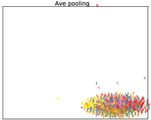
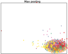
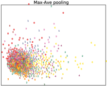
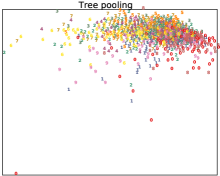
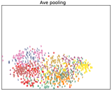
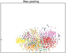
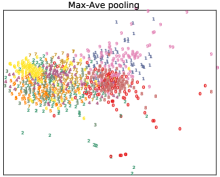
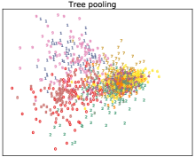
Visualization of network internal representations To gain additional qualitative understanding of the pooling methods we are considering, we use the popular t-SNE [39] algorithm to visualize embeddings of some internal feature responses from pooling operations. Specifically, we again use four networks (one utilizing each of the selected types of pooling) trained on the CIFAR10 training set (see Sec. 5 for architecture details used across each network). We extract feature responses for a randomly chosen -image subset of the CIFAR10 test set at the first (i.e., earliest) and second pooling layers of each network. These feature response vectors are then embedded into 2-d using t-SNE; see Figure A1.
The first row shows the embeddings of the internal activations immediately after the first pooling operation; the second row shows embeddings of activations immediately after the second pooling operation. From left to right we plot the t-SNE embeddings of the pooling activations within networks that are trained with average, max, gated max-avg, and (2 level) tree pooling. We can see that certain classes such as “0” (airplane), “2” (bird), and “9” (truck) are more separated with the proposed methods than they are with the conventional average and max pooling functions. We can also see that the embeddings of the second-pooling-layer activations are generally more separable than the embeddings of first-pooling-layer activations.


| Network layer configurations reported in Tables 1, 2, and 4 of the main paper. | |||||
|---|---|---|---|---|---|
| DSN (baseline) | mixed max-avg | gated max-avg | 2 level tree pool | 3 level tree pool | tree+gated max-avg pool |
| 3x3 (standard) conv | |||||
| 3x3 (standard) conv | |||||
| 1x1 mlpconv | |||||
| 3x3 maxpool | 3x3 mixed max-avg | 3x3 gated max-avg | 3x3 2 level tree pool | 3x3 3 level tree pool | 3x3 2/3 level tree pool |
| 3x3 (standard) conv | |||||
| 3x3 (standard) conv | |||||
| 1x1 mlpconv | |||||
| 3x3 maxpool | 3x3 mixed max-avg | 3x3 gated max-avg | 3x3 maxpool | 3x3 maxpool | 3x3 gated max-avg |
| 3x3 (standard) conv | |||||
| 3x3 (standard) conv | |||||
| 1x1 mlpconv | |||||
| 1x1 mlpconv | |||||
| 8x8 global vote | |||||