Asymmetry of cross correlations between intra-day and overnight volatilities

Abstract

We point out a stunning time asymmetry in the short time cross correlations between intra-day and overnight volatilities (absolute values of log-returns of stock prices). While overnight volatility is significantly (and positively) correlated with the intra-day volatility during the following day (allowing thus non-trivial predictions), it is much less correlated with the intra-day volatility during the preceding day. While the effect is not unexpected in view of previous observations, its robustness and extreme simplicity are remarkable.

It is well known that fluctuations in equity prices traded on any stock exchange are barely correlated, and hardly allow any non-trivial forecasting. This is different for the amplitudes of these fluctuations, called volatilities. If the market is hectic, volatilities are large, and it will take some time until the market has become calm again. With some modern options it is possible to make profits with forecasts for volatilities (although forecasts of signed fluctuations would be more easy to turn into money, if they were possible), whence volatilities have been studied extensively in the econometric literature bouchaud .

As first shown in french ; lockwood , the statistics of volatilities is not uniform. Rather, there is a marked daily structure, with high volatility during the opening hour of the market and a more calm period around noon. This seems to be true for all stock exchanges worldwide. Also, equity prices at the opening of the trading session are in general different from the closing prices on the previous trading day, showing that there is a non-trivial overnight dynamics.

Finally, it has been repeatedly shown that the overnight dynamics is qualitatively different from that during the day Chan ; Edmonds ; Zhong ; Tsiakas ; Chen ; Lee ; Gallo . Various reasons have been proposed for this:

• A foreign equity which is mainly traded on some foreign market (that is open during the night hours of the market studied) reflects mostly its activity in their overnight volatility, and this activity might be very different Chan from the market under consideration.

• The majority of news relevant for fundamental stock price evaluation (company profits, employment rates, general econometric forecasts, wars and natural disasters, …) are released overnight Corral , and there exists a correlation between frequency of news releases and volatilities Edmonds ; Gallo .

• While the market can react during the day to any outside perturbation, it cannot do so during the night, which might also explain the higher volatility immediately after the market opening Gallo .

Since research in economy is mostly driven by the hope for practical applications, it is not surprising that the majority of the above references were concerned with prediction. The general consensus seems that overnight volatility is useful for predicting subsequent intra-day volatility Blanc ; Taylor ; Chicheportiche . This is an important result. But prediction involves a model (GARCH Gallo ; Chen , SEMIFAR Chen , or different versions of the stochastic volatility model (SVM) Tsiakas ; Zhong ; Lee ), and none of the papers cited above report model independent analyses of the raw data themselves. This is so in spite of the fact that data analyses not involving any model and using only elementary methods and minimal assumptions would be most useful for understanding the basic mechanism(s) underlying the phenomena.

It is the purpose of the present short note to provide just such an elementary analysis. The methods used will be completely elementary, and involve nothing more than (Spearman- Press ) cross correlations. Yet the result is striking and completely unexpected, as far as significance and robustness are concerned. We should point out that an extensive statistical study of intra-day and overnight returns and volatilities was recently made in Wang , but since that analysis was not guided by any theoretical considerations, the effect described below was missed.

Let us use the index $k$ to count trading days (i.e., skipping weekend and other non-trading days), and denote by $o_{k}$ and $c_{k}$ the opening and closing prices of one particular equity. Intra-day log-returns of this equity are defined as

$$d_{k}=\ln\frac{c_{k}}{o_{k}}\;,$$ (1)

while overnight log-returns are

$$n_{k}=\ln\frac{o_{k}}{c_{k-1}}\;.$$ (2)

Thus overnight returns are indexed by the index of the following day. In case of weekends and holidays the over-“night” returns include all changes during the entire non-trading period. Volatilities are in principle defined through the variances of log-returns as observed over an extended time span. But when discussing them on a fine grained temporal scale, they are usually replaced by the absolute values of the log-returns (see e.g. footnote 11 in Tsiakas ). We will follow this usage.

Figure 1: Historical time series of stock intra-day (panel a) and overnight (panel b) returns for the MDAX index.

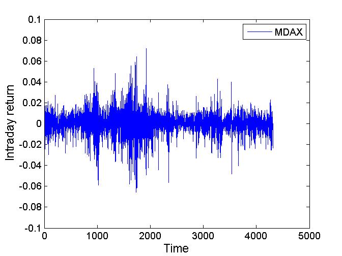
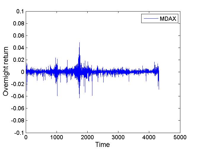
The data we studied consists of 21 individual stocks traded at various stock exchanges (Exxon, Shell, General Electric, Ford, Goldmann-Sachs, Bank of America, Citigroup, IBM, Microsoft, Cisco, AIG, BP, Caterpillar and Ford all traded at NYSE; Siemens, Deutsche Bank, Lufthansa, VW and Bayer traded in Frankfurt; and Sony & Mitsubishi traded in Tokyo) and 10 market indices and exchange-traded funds (TecDax, MDax, DAX, Dow Jones, S&P 100, Nasdaq, EuroSTOXX 50, SIM, S&P/ASX and PowerShares QQQ). They were mostly downloaded from Yahoo (https://finance.yahoo.com/), the rest from finanzen.net (http://www.finanzen.net). The time sequences cover between 10.4 and 45 years, with between 2612 and 13478 data points. Before using them, we cleaned them from some of their artifacts (missing data, wrong data, …), but not of all. For instance, we did not remove jumps due to stock splitting. After cleaning, they show the typical features well known from previous analyses, such as fat tails, short-time correlations in the returns, and long-time correlations in the volatilities. For typical examples, see Fig. 1. Notice that these data still have outliers (mostly negative, due to crashes, bad annual reports,…). The negative outliers occur mostly for the overnight returns, consistent with the previous observation that negative news are disseminated mostly when the markets are closed. The long autocorrelations of the volatilities are seen both for daytime and overnight.

Figure 2: Data for 31 equities. Each dot corresponds to one equity. The Spearman correlation between intra-day volatilities and overnight volatilities during the subsequent night are plotted on the x-axis, while the correlations with the preceding night are on the y-axis.

Our main concern is with cross-correlations between intra-day and overnight volatilities. Due to the artifacts, irregularities, and strong non-stationarity in the data, we did not use simple Pearson coefficients. Instead we used Spearman coefficients Press . Being based on rank statistics, these are known to be much more robust. Indeed, the results shown below would have been much less clearly visible had we used Pearson coefficients. Alternatively we could also have used Kendall’s $\tau$ Kendall or mutual informations Cover , both of which are known to be similarly robust.

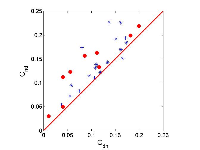
Our main results are shown in Figs. 2 and 3, In Fig. 2 we show for each equity two cross-correlations between the ranks $r_{d_{k}}$ and $r_{n_{k}}$ of the two volatilities $|d_{k}|$ and $|n_{k}|$:

$$C_{nd}=\frac{\langle r_{d_{k}}r_{n_{k}}\rangle-\langle r_{d_{k}}\rangle\cdot\langle r_{n_{k}}\rangle}{\sigma_{d}\;\sigma_{n}}$$ (3)

is the rank correlation between the intra-day volatility and the volatility during the preceding night ($\sigma_{d}$ and $\sigma_{n}$ are the square roots of the rank variances), while

$$C_{dn}=\frac{\langle r_{d_{k}}r_{n_{k+1}|}\rangle-\langle r_{d_{k}}\rangle\cdot\langle r_{n_{k}}\rangle}{\sigma_{d}\;\sigma_{n}}$$ (4)

gives the analogous correlation with the following night. We see that in all cases

$$C_{nd}>C_{dn}.$$ (5)

For some equities the difference is small, but for others it can be more than a factor of two. In only one case the inequality was violated. Thus the overnight volatility is much stronger correlated with the volatility during the following day than during the preceding day. Otherwise said, overnight volatilities seem to influence strongly what goes on during the following trading day, but do not seem to be strongly influenced by what was going on during the day before footnote .

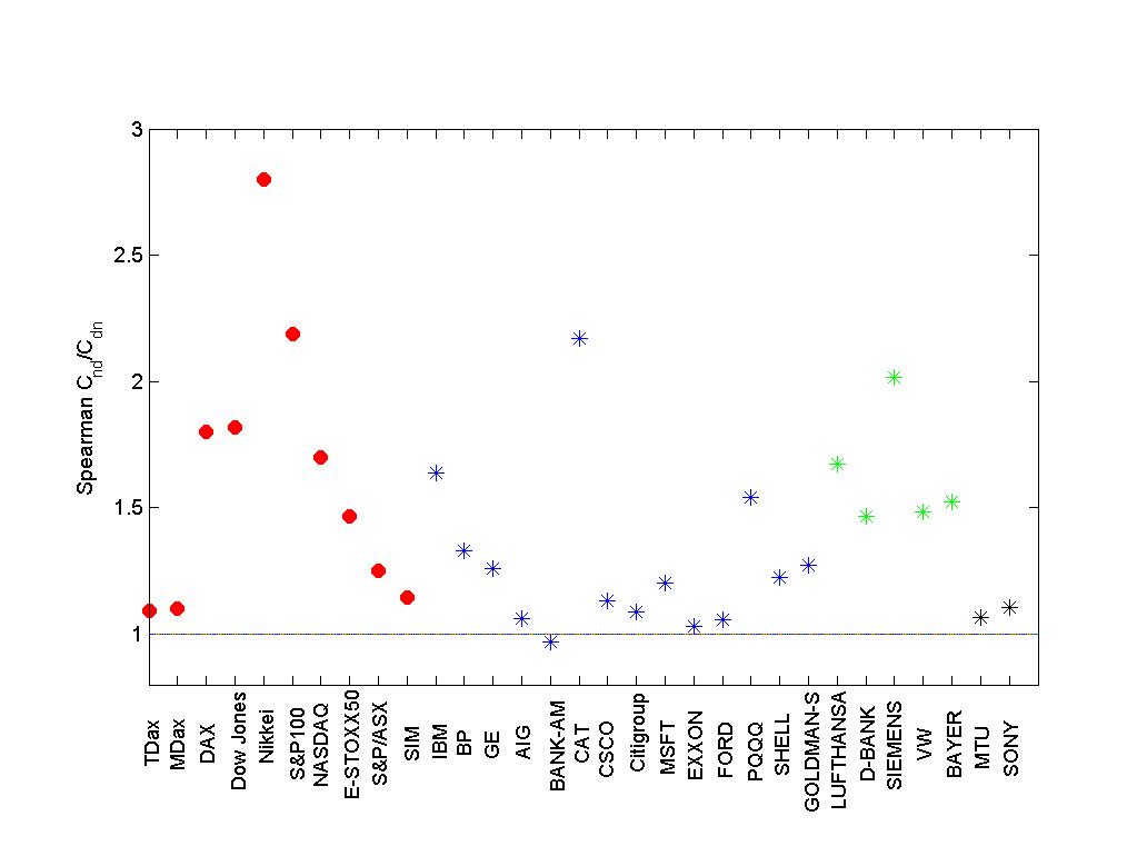
The ratios $C_{nd}/C_{dn}$ for the equities used in Fig. 2 are plotted also in Fig. 3, where we have also specified the equities. The first 10 entries in this figure are market indices, while the others correspond to individual stocks. We see no big differences, except that aggregated indices show a somewhat stronger effect. There are also no noticeable differences related to the place where the equity is traded, to the length of the time series, and – in case of individual stocks – to the type of company.

Figure 3: Ratios $C_{nd}$/ $C_{dn}$ for the 31 equities and indices shown also in Fig. 2. For stocks, the colors indicate the stock exchanges where they are traded.

At first sight this strong asymmetry looks very strange, in particular since time asymmetry is usually considered to be very weak in financial data. Many popular models (most noticeably all models of the ARCH family) are time symmetric by construction, and where time asymmetry is seen Zumbach ; Blanc it is only seen in very special observables. But our findings are indeed compatible with previous analyses lockwood ; Chan ; Edmonds ; Zhong ; Tsiakas ; Chen ; Lee ; Gallo : While the intra-day price dynamics is largely influenced by ‘chartist’ behavior, the overnight dynamics is mostly influenced by facts exogenous to the stock market (or at least not directly related to the day-to-day price evolution of the considered equity) and thus of ‘fundamentalist’ nature. What our results suggest is that ‘fundamentalist’ information is more useful in prediction than ‘chartist’ information.

The present analysis cannot of course specify which of the possible external influences (foreign stock markets, company performance reports, news about general economic indicators such as employment rates and forecasted economic growth, wars, economic crises, natural disasters, …) is of greatest importance for the overnight dynamics, but such information could possibly be obtained by performing a larger study similar to the present one in which equities are grouped according to business sectors, stock exchanges, trading volume, bull versus bear markets, etc. Another improvement suggested by our analysis could consist in replacing the simple cross correlations by partial correlations or by transfer entropies Schreiber , testing in this way for linear or non-linear Granger causality Barnett . It would be of interest to see whether the asymmetry found in the present paper is also present at larger time scales, by comparing day/night to night/day results between more distant nights and days.

Finally, with the hindsight gained from this analysis, we might also turn to signed returns (in contrast to volatilities) and test whether some parts of a full 24 hours day have more influence on later periods than others. The very fact that different regions in the phase space of a recurrent system can have different powers of predictability has been known for long time Farmer .

We thank Andreas Klümper for discussions and for carefully reading the manuscript, and Jean-Philippe Bouchaud and Spyros Skouras for comments. R.Z. thanks Holger Kantz and Peter Fulde for support and discussions. P.G. thanks Derek Belle for collaboration during an early stage of the work and Amer Shreim for discussions.

References

- (1) J.-P. Bouchaud and M. Potters, Theory of Financial Risk and Derivative Pricing: From Statistical Physics to Risk Management (Cambridge Univ. Press, Cambridge U.K., 2003).
- (2) K.R. French and R. Roll,”Stock Return Variances: The Arrival of Information and the Reaction of Traders”, Journal of Financial Economics 17, 5-26 (1986).
- (3) L.J. Lockwood and S.C. Linn, “An examination of stock market return volatility during overnight and intraday periods, 1964-1989”, Journal of Finance 45, 591-601 (1990).
- (4) K. Chan, M. Chockalingam and K.W.L. Lai, “Overnight information and intraday trading behavior: evidence from NYSE cross-listed stocks and their local market information”, J. Multinat. Financial Management 10, 495-509 (2000).
- (5) R.G. Edmonds and A.M. Kutan, “ Is Public Information Really Irrelevant in Explaining Asset Returns?”, Economics Letters bf 76, 223-229 (2002).
- (6) Z. Zhong, “The Predictability of Overnight Information”, Dissertations and Theses Collection. Paper 46. http://ink.library.smu.edu.sg/etd-coll/46.
- (7) I. Tsiakas, “Overnight information and stochastic volatility: A study of European and US stock exchanges”, Journal of Banking & Finance 32, 251-268 (2008).
- (8) C.-H. Chen, W.-C. Yu and E. Zivot, “Predicting Stock Volatility Using After-Hour Information”, unpublished (2009).
- (9) C.-C. Lee and C.-S. Wang, “Overnight information and stochastic volatility: A study of Asia stock markets” (in Chinese), Master thesis, Ming Chuan University (2009).
- (10) G.M. Gallo and B. Pacini, “Early news is good news: the effects of market opening on market volatility”, Studies in Nonlinear Dynamics and Economics 2, 115-131 (1998).
- (11) W. Del Corral, D. Colwell, D. Michayluk and L.A. Woo, “News releases when the markets are closed”, unpublished, University of Technology, Sidney (2003).
- (12) P. Blanc, R, Chicheportiche, and J.-P. Bouchaud, “The fine structure of volatility feedback II: Overnight and intra-day effects”, Physica A 402, 58 (2014).
- (13) N. Taylor, “The Predictive Value of Temporally disaggregated Volatility: Evidence from Index Futures Markets, J. Forecast. 27, 721 (2008).
- (14) R. Chicheportiche, “Non-linear Dependencies in Finance”, PhD Thesis, Ecole Centrale des Arts et Manufactures, Paris (2013).
- (15) W.H. Press et al., “Numerical recipes: The art of scientific computing”, 3rd edition (Cambridge University Press, 2007).
- (16) F. Wang, S.-J. Shieh, S. Havlin, and H. E. Stanley, “Statistical analysis of the overnight and daytime return”, Phys. Rev. E 79, 056109 (2009).
- (17) M. Kendall, ”A New Measure of Rank Correlation”. Biometrika 30, 8 (1938).
- (18) T.M. Cover and J.A. Thomas, “Elements of information theory”, (John Wiley & Sons, 2012).
- (19) Notice in this context that the title of Zhong is wrong. That paper is concerned with the usefulness of overnight information for prediction, not with its predictability.
- (20) G.O. Zumbach, “Time reversal invariance in finance”, Quant. Finance 9, 505 (2009).
- (21) T. Schreiber, “Measuring information transfer”, Phys. Rev. Lett. 85, 461464 (2000).
- (22) Lionel Barnett, Adam B. Barrett, and Anil K. Seth, “Granger Causality and Transfer Entropy Are Equivalent for Gaussian Variables”, Phys. Rev. Lett. 103, 238701 (2009).
- (23) R.J. Deissler and J.D. Farmer, “Deterministic Noise amplifiers”, Physica D 55, 155 (1992).