Numerical study of DNA denaturation with self-avoidance: pseudo-critical temperatures and finite size behaviour.

Abstract

We perform an extensive numerical study of the disordered Poland-Scheraga (PS) model for DNA denaturation in which self-avoidance is completely taken into account. In complement to our previous work, we focus here on the finite size scaling in terms of pseudo-critical temperatures. We find notably that the mean value and the fluctuations of the pseudo-$T_{c}$ scale with the same exponent, the correlation length exponent $\nu_{r}$ (for which we provide the refined evaluation $\nu_{r}=2.9\pm 0.4$). This result (coherent with the typical picture that describes random ferromagnets, when disorder is relevant) is at variance with numerical results reported in the literature for the PS model with self-avoidance, leading to an alternative scenario with a pseudo first order transition. We moreover introduce a crossover chain length $N^{*}$, which we evaluate, appropriate for characterizing the approach to the asymptotic regime in this model. Essentially, below $N^{*}$, the behaviour of the model in our study could also agree with such alternative scenario. Based on an approximate prediction of the dependence of $N^{*}$ on the parameters of the model, we show that following the choice of such parameters it could be not possible to reach the asymptotic regime in practice. In such context it becomes then possible to reconcile the apparently contradictory numerical studies.

PACS: 64.60.Fr    Equilibrium properties near critical points, critical exponents
PACS: 82.39.Pj   Nucleic acids, DNA and RNA bases
PACS: 89.75.Fb   Structures and organization in complex systems

1 Introduction

The study of disordered systems has attracted a wide interest in statistical physics. Numerical studies appear of critical importance in the field, as the handling of disorder can be difficultly amenable to analytic treatments. In any case numerical approaches appear to be the best suited for capturing details of interesting behaviours, such as those related to finite-size effects.

In this background, the disordered Poland-Scheraga (PS) model for DNA denaturation stands as a privileged model, following several perspectives: i) as an instance of the so-called ”helix-coil transition” models, the model is designed to capture one of the most basic phenomenon in molecular biology, relative to the opening of the double-helix; ii) to render the helix-coil transition model more realistic, the PS model takes into account intrinsic long-range effects (associated with the weights of the loops in the coiled state), which can extend throughout the length of the system; iii) originally specifically associated with the model, numerical methods were developed to handle the statistical mechanics problem with long-range effects very efficiently, allowing to consider system sizes which are orders of magnitude larger than what would be possible with Monte-Carlo methods.

With this respect, the PS model of DNA denaturation with self-avoidance is of particular interest, notably as it belongs to a more general class of polymer models for which the question of disorder relevance has been definitely answered only recently [1, 2, 3], in a probabilistic mathematical framework. More precisely, for this class of models, disorder is predicted to be relevant, the transition being expected to be at least of second order. In such context, the numerical findings of our previous work [4], relying on a standard finite size scaling analysis, indeed agree with a smooth transition, suggesting a value $\nu_{r}=2.9\pm 0.6$ for the correlation length exponent.

In contrast, other studies of the DNA denaturation model with self-avoidance [5, 6] instead supported, both on numerical and theoretical grounds, the possibility of a pseudo first order transition. Such scenario could be in fact accommodated within theoretical descriptions of relevant models, such as random ferromagnets, with, in any case, disorder expected to be relevant from the Harris criterion point of view. Briefly, within this picture, one predicts the presence of two correlation lengths, which can be evidenced numerically in particular by an analysis in terms of (appropriately defined, sequence-dependent) pseudo-critical temperatures, since the two corresponding exponents should rule the scaling of the mean value and that of the fluctuations of the pseudo-$T_{c}$, respectively. In detail, in these studies, the exponent related to the fluctuations was found to have the value 2, thus coherent with a second order transition (and, from this point of view, with disorder relevance), whereas the one related to the mean value was found to have the value 1, thus, concomitantly, denoting a pseudo first order character of this transition.

In fact, based on recent mathematical findings, [1, 2, 3] it would be possible to rule out such scenario for the thermodynamic limit behaviour of the present model. This situation is further reinforced by the prediction, within the same probabilistic mathematical framework, of a thermodynamic limit behaviour governed by a single correlation length [7].

The general situation as described above motivates the present extensive numerical study, in the prolongation of our previous work, since it appears desirable to clarify the overall situation relative to the theoretical/numerical results, all the more that in [5, 6] extremely large sizes were considered (up to $N=2\cdot 10^{6}$), which should in principle be appropriate for reflecting the thermodynamic limit properties evidenced in the theoretical studies. It is in this direction that we perform here a finite size scaling analysis in terms of pseudo-critical temperatures. In any event, for the present peculiar model, displaying strong corrections to scaling and a slow approach to the asymptotic regime [4], a general deeper understanding of the finite size behaviour is of interest both from the physics and biological points of view.

More precisely, we tackle a hitherto unaddressed problem, relative to the definition of appropriate pseudo-critical temperatures in the presence of multiple peaks in quantities such as the specific heat and the susceptibility, which represent as a matter of fact a salient feature of the underlying biological model. Focusing on the strongly non self-averaging behaviour of observables at the critical point, we find that the pseudo-$T_{c}$ can be appropriately defined as the position of the absolute maximum of susceptibility, for a given sequence. We notably show that the mean value and the fluctuations of this observable scale with the same exponent, thereby confirming that the asymptotic regime is reached in our case. At variance with the numerical findings in [5, 6], the present result is thus coherent with the typical picture describing random ferromagnets when disorder is relevant.

In order to understand in depth the finite size behaviour, we further perform an extensive analysis of the loop-length probability distribution, at different temperatures. The behaviour of this observable reveals in a particularly evident way the presence of a crossover chain length $N^{*}$. Indeed, this quantity appears to be particularly appropriate for characterizing the slow approach to the asymptotic regime in the present model. Basically, for chain lengths below $N^{*}$, in our study the behaviour of the model would also agree with the scenario of a pseudo first order transition. As a matter of fact, the evaluation of $N^{*}$ in our case, and the approximate prediction within a phenomenological framework of its dependence on the parameters of the model, allows us to resolve the possible paradox concerning contradictory numerical findings as described above. We show notably that, with the choice of parameters in [5, 6], it could be not possible to reach the asymptotic regime in practice.

The paper is organized as follows: we briefly review the general background in Section 2; we introduce the model and the observables in Section 3, where we first summarize known results for the pure case (3.1), we introduce the disordered model, by defining the different parameters entering in the computation of the partition function by means of the recursive equations (3.2), we describe possible scenarios within the framework of the analysis in terms of pseudo-critical temperatures, clarifying the different ways of averaging considered (3.3), we recall the approximation used for the power law and the details of the numerical implementation of the computations (3.4); we present and discuss our results on the analysis with the pseudo-critical temperatures in Section 4, where we start from the possible definitions of this observable (4.1), we study the scaling of its mean value and of its fluctuations (4.2), we compare different ways of averaging (4.3), and we show data on the non self-averageness parameter related to the susceptibility (4.4); we present and discuss our results on the characterization of the finite size behaviour in Section 5, where we outline the presence of the crossover chain length $N^{*}$ by the detailed study of data on the loop-length probability distribution (5.1), and we discuss our attempt to roughly estimate the dependence of this quantity on the parameters of the model (5.2); finally, we present our conclusions in Section 6.

2 General background

A realistic model for the DNA denaturation transition (taking into account the entropic weights of the loops) was introduced by Poland and Scheraga (PS) [8, 9, 10], to account for experimental melting curves, allowing their prediction [11, 12, 13]. Models for DNA denaturation were originally developed in the context of fundamental biological questions, relevant notably to the possible overlap between physical (helix/coil) and genetic (coding/non-coding) segmentations of genomic sequences (for an overview see [14, 15, 16, 17], and references therein). Furthermore, the PS model appeared to be also of interest in the context of statistical mechanics: the segmentation of the DNA chain into helix/coil regions represents an instance of an almost uni-dimensional system [18], which can undergo a phase transition because of the long range effects, associated with the entropic weights of the loops (with the loop-length probability distribution described by an exponent $c_{p}$).

In fact, upon introducing the $c_{p}$ value appropriate for taking into account loop self-avoidance effects, larger than the one describing a random walk loop, it was hypothesized early on [10] that a more complete handling of self-avoidance, taking also into account the self-avoidance of the chain with itself, would lead to an even larger value for the exponent, and correspondingly to a sharper transition in the $pure$ case (homogeneous sequence). However the confirmation of this hypothesis [19, 20] had to await conformal field theory results [21], showing that the correct loop-length probability distribution exponent associated to a self-avoiding loop embedded in a self-avoiding chain in three dimensions fulfills the condition $c_{p}>2$, leading to a first order singularity (with corresponding correlation length critical exponent $\nu_{p}=1$). The first order character of the transition was initially observed in a numerical study of a on-lattice homogeneous model consisting of two interacting self-avoiding walks (SAWs) [22], with the numerical estimation ($c_{p}\simeq 2.15$) in this case [23, 24, 25] in very good agreement with the theoretical predictions mentioned above.

It can be noted that, because of the difference between the link energies of $\varepsilon_{AT}$ (Adenine-Thymine) and $\varepsilon_{GC}$ (Guanine-Cytosine) base pairs, DNA is an intrinsically $random$ system in which the disordered variables are $quenched$, in the sense that the composition of the sequence in terms of base pairs does not vary during the denaturation process. Accordingly, to understand the behaviour of the system in the thermodynamic limit of chain length $N\rightarrow\infty$ in the canonical ensemble, it is necessary to evaluate the quenched free energy density, by taking the average (over the random variables) of the logarithm of the partition function for the generated disordered configurations. However, it appears particularly hard to handle such quantity analytically [26]. In fact, whereas the equilibrium properties of the pure system were well understood, it was only recently that probabilistic mathematical approaches [1, 2, 3, 7] allowed to definitely demonstrate that general theoretical results relative to the relevance of disorder [27, 28, 29, 30] do also hold for the depinning transition of disordered copolymers. This conclusion holds in particular for the PS models with $c_{p}>2$, despite the fact that such models are instances of peculiar first order transitions, characterized by the presence of a diverging correlation length, in a system in which the disorder couples to only one of the two phases. Accordingly, such cases are expected to exhibit a random fixed point corresponding to a second order or possibly smoother transition, described by a correlation length critical exponent $\nu_{r}\geq 2/d=2$ (with, to our knowledge, no theoretical prediction available for the $\nu_{r}$ value).

Whereas these theoretical determinations are appropriate to account for the behaviour of the model in the thermodynamic limit, in the experimental situation we are typically concerned with the thermal denaturation of DNA molecules of specific sequence and given finite size. In such context it is implicitly assumed that the intrinsic disorder is at the origin of the well-known multi-step behaviour of the density of closed base pairs, $\theta(\{\varepsilon_{i}\},N,T)$, the order parameter of the transition as accessible through optical absorbance measurements. It is then classical to analyze the derivative of this quantity with respect to temperature ($d\theta(\{\varepsilon_{i}\},N,T)/dT$), which displays distinct peaks as reflecting the multi-step behaviour. At this level, from the statistical mechanics point of view, the first order character of the transition in the pure case is in agreement with the observation that the steps are typically very steep, hence the corresponding peaks very sharp. On the other hand, the fact that GC-rich regions tend to open at higher temperatures than AT-rich ones, suggests in a particularly evident way the possibility of non self-averageness for densities of extensive quantities, in the sense that the positions and the characteristics of the steps, and of the corresponding peaks, are strongly sequence-dependent.

On general grounds, it is accordingly expected [31] that, for $N\rightarrow\infty$, the temperature range where such behaviour is observed shrinks around the critical temperature $T_{c}$, the transition being rounded. In fact, it is only at the critical point that the presence of a diverging correlation length breaks down the argument usually used to demonstrate self-averageness of densities of extensive quantities [32], built on the description of the system as consisting of weakly interacting sub-systems. However the validity of such picture is not obvious for the present almost one-dimensional polymer model, in which self-avoidance represents an infinite range interaction.

In the background of the recent mathematical findings [1, 2, 3, 7], it is expected that the effect of disorder on this peculiar first order transition would be the same than the one predicted theoretically for random ferromagnets [31] (as further confirmed numerically in [33] for site dilute Ising models), with in particular the mean value and the fluctuations of an appropriately defined pseudo-critical temperature scaling with the same exponent. Nevertheless it is highly desirable for the present model to further assess numerically this picture, in order notably to better understand the way in which relevance of disorder becomes manifest, as tackled at the finite size level.

3 Model and observables

3.1 The pure case

For the sake of completeness, we first recall briefly the salient features of the homogeneous on-lattice model which was introduced in [22]: two SAWs with the same origin on a $3d$ cubic lattice, obeying the simple rule that two monomers can occupy the same lattice point (gaining a coupling energy $\varepsilon$) if and only if their positions along the two chains are identical. The thermal variables describing the system can be represented by the ensemble of the $\{s_{i}\}$, with $s_{i}=0$ if the base pair in position $i$ is in the open state and $s_{i}=1$ if it is in the closed state. The possible configurations are only the ones allowed by self-avoidance, thus introducing an infinite range interaction of entropic nature in an almost uni-dimensional Ising model [18]. The energetic contribution of a given configuration to the Boltzmann weight of the “spins” $\{s_{i}\}$ (hence the associated Hamiltonian) is then simply written as ${\cal H}=-\varepsilon\sum_{i=1}^{N}s_{i}$. It can be noticed that $\varepsilon$ enters in the partition function only through the ratio $\varepsilon/T$, allowing thus to set $\varepsilon=1$ without loss of generality.

This model can in particular be assimilated to a homogeneous DNA denaturation transition model à la PS [8, 9, 18, 10, 22], in which the two chains represent the two strands of the double helix, allowing for one free-end but not base-pair mismatches. It is then interesting to notice that self-avoidance is fully taken into account in the on-lattice numerical simulations, by design. In fact, it is found [22] that, in the thermodynamic limit of infinite chain length $N\rightarrow\infty$, the model undergoes a first order phase transition with a discontinuity in the order parameter, the density of closed base pairs $\theta(T)=\frac{1}{N}\sum_{i=1}^{N}\langle s_{i}\rangle$ ($\langle\cdot\rangle$ holding for the $thermal$ average), which varies abruptly from zero value at high temperature to a finite value below the critical temperature $T_{c}$. The properties of the system are better grasped in the behaviour of the loop-length probability distribution [19, 20, 23, 24, 25]:

$$P(T,l)\propto\frac{e^{-l/\xi(T)}}{l^{c_{p}}},$$ (1)

in which appear both the exponent $c_{p}$, describing the purely algebraic decay of $P(T,l)$ at the critical point, and the correlation length $\xi(T)$. In the considered case, in which we allow for one free-end, it could be necessary in principle to take into account an additional length scale, corresponding to the distance between end points [22, 6]. Nevertheless, such requirement should be basically considered to be associated with a boundary condition [20], therefore not influencing the thermodynamic limit properties of the model.

In general, upon solving these models in the grand canonical ensemble, the succession of closed segments (helix) and open loops (coil regions) sums up as a geometric series [18]. However, in the present case, such treatment amounts to neglect the self-avoiding interactions between different segments and loops, which can be taken into account more correctly by the appropriate renormalization of $c_{p}$ [19, 20]. Transitions in homogeneous PS models are then found to be of first order, both in $d=3$ and in $d=2$. Accordingly, they are characterized by an order parameter critical exponent $\beta_{p}=0$, i.e. a discontinuity in $\theta(T)$, but also by the presence of a diverging correlation length, with related critical exponent $\nu_{p}=1$ (since renormalization leads to $c_{p}>2$). In the theoretical framework of almost uni-dimensional phase transitions this correlation length is to be interpreted as the longitudinal one [18, 20], corresponding to the mean loop length $\langle l\rangle$ along the chain, whose variance diverges. More in detail, based on conformal field theory results [21], the theoretical prediction in $d=3$ for a self-avoiding loop embedded in a self-avoiding chain [19, 20] leads to a $c_{p}$ value between 2.115 and 2.22, in very good agreement with the value $c_{p}\simeq 2.15$ found in numerical study of the on-lattice SAW DNA model [23, 24, 25].

The behaviours at criticality expected for the singular parts of the various thermodynamic quantities in PS models are summarized in [Tab. 1], defining implicitly the order parameter critical exponent $\beta_{p}$, the correlation length critical exponent $\nu_{p}$, and the specific heat critical exponent $\alpha_{p}$ (the label $p$ is to distinguish the pure $p$ case from the random $r$ one), all of them being expressible as functions of the sole variable $c_{p}$. It can be noticed in particular that here the energy behaves as the order parameter, hence the singular part of the specific heat behaves as the one of the derivative of the order parameter with respect to the temperature, as well as to that of its derivative with respect to $\varepsilon$, i.e. to the singular part of the susceptibility. Moreover $T_{c}$ is to be reached from the low temperature phase, as the thermodynamic limit correlation length is infinite in the whole phase $T>T_{c}$ (both with and without one free-end allowed).

lim_T →T_c^-θ(T) ∝(T_c-T)^β_p β_p = { 0 for c_p ≥2(2-c_p)/(c_p-1) for c_p ¡ 2 lim_T →T_c^-ξ(T) ∝(T_c-T)^-ν_p ν_p = { 1 for c_p ≥21/(c_p-1) for c_p ¡ 2 lim_T →T_c^-dθ(T)dT ∝(T_c-T)^-α_p α_p = 1-β_p=2-ν_p lim_T →T_c^-P(T,l) ∝1lcp

Table 1: Behaviours at criticality of the singular parts of the relevant thermodynamic quantities in the model, which involve only one independent critical exponent (see text for details).

It can be useful to recall, in order to better specify the link between the on-lattice $3d$ SAW DNA model and the associated PS one, that the transition in the grand canonical ensemble occurs in fact at a tri-critical point in the fugacity-temperature plane (see [22] and references therein), better described by the crossover exponent $\phi_{p}=\nu_{g}^{3d}/\nu_{p}^{3d}$, where $\nu_{g}^{3d}=1/{\cal D}$ is the geometrical correlation length critical exponent (given by the inverse of the fractal dimension ${\cal D}$ of the $3d$ SAW), whereas $\nu_{p}^{3d}$ corresponds to the thermal correlation length critical exponent. Accordingly, the relation $\alpha_{p}=2-\nu_{p}$ (which in PS models corresponds simply to a particular case of the well known relation $\alpha_{p}=2-d\nu_{p}$ in $d=1$), is the analogous within the almost uni-dimensional framework to the $3d$ relation $\alpha_{p}=2-{\cal D}\nu_{p}^{3d}=2-\nu_{p}^{3d}/\nu_{g}^{3d}=2-1/\phi_{p}$ (with the first order case corresponding to $\phi_{p}=1$, i.e. $\nu_{p}^{3d}=\nu_{g}^{3d}$). On the other hand, the definition of $P(T,l)$ given by Eq. (8) implicitly refers to the unidimensional structure of the system (with $l$ the loop length along the chain), and accordingly the corresponding correlation length critical exponent is given by $\nu_{p}={\cal D}\nu_{p}^{3d}=1/\phi_{p}$. It is worth noting that the fractal dimension ${\cal D}$ is by definition the same in the presence of disorder.

3.2 The random case

The DNA is intrinsically a disordered system, because of the difference in the coupling energies between $AT$ and $GC$ base pairs. To account for disorder it is then necessary to introduce a coupling dependent on the position $i$ of the base pair along a given sequence, $\varepsilon_{i}$, writing accordingly:

$${\cal H}=-\sum_{i=1}^{N}\varepsilon_{i}\>s_{i}.$$ (2)

It is then important to distinguish thermal averages, $\langle(\cdot)\rangle$ (over the thermal variables $\{s_{i}\}$), from disorder averages, $\overline{(\cdot)}$ (over the different possible realizations of the quenched random variables $\{\varepsilon_{i}\}$, i.e. the different possible sequences).

A simple choice for the couplings [34, 5, 6, 4] consists in considering identically distributed independent random variables $\{\varepsilon_{i}\}$, following the binomial law:

$$P(\varepsilon_{i})=\frac{1}{2}\left[\delta(\varepsilon_{i}-\varepsilon_{AT})+\delta(\varepsilon_{i}-\varepsilon_{GC})\right],$$ (3)

which assumes the same mean $AT$ and $GC$ contents, leaving free the choice of the value for the energy ratio parameter $R=\varepsilon_{GC}/\varepsilon_{AT}$. In the present work, as in [4], we study the PS model corresponding to the disordered on-lattice $3d$ SAW DNA in [34], with $R=2$ (obtained by taking $\varepsilon_{GC}=2$ and $\varepsilon_{AT}=1$).

In terms of recurrent evaluations, for a system of length $n+1$ with both base pairs $i=1$ and $i=n+1$ in the closed state ($s_{1}=s_{n+1}=1$), the forward partition function $Z^{f}(\{\varepsilon_{i}\},n+1,T)$, which sums the contributions of all the configurations weighted by their Boltzmann factors, is obtained from $Z^{f}(\{\varepsilon_{i}\},n,T)$ as:

$$Z^{f}(\{\varepsilon_{i}\},n+1,T)=e^{(\beta\epsilon_{n+1}-\log\mu)}\left[Z^{f}(\{\varepsilon_{i}\},n,T)+\sum_{n^{\prime}=1}^{n-1}\frac{Z^{f}(\{\varepsilon_{i}\},n^{\prime},T)}{[2(n-n^{\prime}+1)]^{c_{p}}}\right].$$ (4)

Similarly, the backward partition function $Z^{b}(\{\varepsilon_{i}\},n-1,T)$ is obtained as:

$$Z^{b}(\{\varepsilon_{i}\},n-1,T)=e^{(\beta\epsilon_{n-1}-\log\mu)}\left[Z^{b}(\{\varepsilon_{i}\},n,T)+\sum_{n^{\prime}=n+1}^{N}\frac{Z^{b}(\{\varepsilon_{i}\},n^{\prime},T)}{[2(n^{\prime}-n+1)]^{c_{p}}}+1\right],$$ (5)

where the last term in the expression between parentheses is for taking into account the allowance for one free-end.

The implementation of the model also implies a choice for the value of the connectivity constant $\mu$: as well known, $\mu=2d$ for a $d$-dimensional random walk on a hyper-cubic lattice and $\mu\simeq 4.7$ for a $3d$ SAW on a cubic lattice, leading to $\log\mu\simeq 1.54$ in our case [4].

e({ε_i},N,T) ≡- 1N ∑_i=1^N ε_i ⟨s_i ⟩ (energy density) c({ε_i},N,T) ≡ 1T2 ∂∂Te({ε_i},N,T) (specific heat) θ({ε_i},N,T) ≡ 1N ∑_i=1^N ⟨s_i ⟩ (order parameter) χ({ε_i},N,T) ≡ { 1N[⟨(∑_i=1^N s_i )^2 ⟩- (⟨∑_i=1^N s_i ⟩)^2 ]T [∂∂ϵATθ({ε_i},N,T) + ∂∂ϵGCθ({ε_i},N,T) ] (susceptibility)

Table 2: Definition of relevant thermodynamic observables in the model.

The total partition function for a sequence $\{\epsilon_{i}\}$ of length $N$ is given by:

$$Z(\{\varepsilon_{i}\},N,T)=\sum_{n=1}^{N}Z^{f}(\{\varepsilon_{i}\},n,T)=Z^{b}(\{\varepsilon_{i}\},1,T).$$ (6)

Therefore, it is possible to evaluate the probability for a base pair in position $n$ to be in the closed state (i.e. the thermal average $\langle s_{i}\rangle$):

$${\cal P}(\{\varepsilon_{i}\},N,T,n)=\langle s_{i}\rangle=\frac{Z^{f}(\{\varepsilon_{i}\},n,T)Z^{b}(\{\varepsilon_{i}\},n,T)}{Z(\{\varepsilon_{i}\},N,T)\exp({\beta\epsilon_{n}-\log\mu})},$$ (7)

from which relevant thermodynamic observables (whose definitions are recalled in [Tab. 2]) are obtained easily. It is worth noticing that results in [34, 4] are in agreement with a situation in which, also in the presence of disorder, the order parameter behaves as the energy (with $\beta_{r}=\nu_{r}-1$), and the susceptibility as the specific heat (with $\alpha_{r}=2-\nu_{r}$). Under such conditions only one independent critical exponent needs to be evaluated.

Finally, we recall that the loop-length probability distribution, apart from the normalization constant (imposing $\sum_{l}P(\{\varepsilon_{i}\},T,N,l)=1$), can be evaluated as:

$$P(\{\varepsilon_{i}\},N,T,l)\propto\frac{1}{l^{c_{p}}}\sum_{n}\frac{Z^{f}(\{\varepsilon_{i}\},n,T)Z^{b}(\{\varepsilon_{i}\},n+l+1,T)}{Z(\{\varepsilon_{i}\},N,T)}.$$ (8)

This expression further highlights the fact that in the present model $c_{p}$ corresponds to an $input$.

In this context, the simplest picture describing the random fixed point, in agreement with the numerical results in [34, 4], is the one in which in the thermodynamic limit:

$$P(T,l)=\lim_{N\rightarrow\infty}\overline{P(\{\varepsilon_{i}\},N,T,l)}\propto\frac{e^{-l/\xi(T)}}{l^{c_{r}}},$$ (9)

Accordingly, as in the pure case (see Eq. (8)), the average loop-length probability distribution is expected to display a purely algebraic decay at the critical point, where the average correlation length $\xi(T)$ diverges. This purely algebraic decay is described by the random critical exponent $c_{r}$, which in the case of a smooth transition should be linked to the correlation length critical exponent $\nu_{r}$ by the relation $c_{r}=1+1/\nu_{r}$: the same kind of relation which is known to be valid for the pure system, for $c_{p}<2$.

3.2.1 Implementation of the PS model with self-avoidance in various numerical studies

The PS model considered here corresponds in a detailed way to the on-lattice $3d$ disordered SAW DNA model, with the same distribution of the coupling energies, studied numerically in [34]. In this work, by means of parallel computing, it was possible to collect sufficient statistics up to chain lengths $N=800$. Simulations were extensively performed in the case $R=2$, considering also different values of $R$. With such choices of the parameters, applying standard finite size scaling, it was found that the length scale considered was not large enough for reaching conclusive results.

More in detail, the estimations obtained for $\phi_{r}$, which appeared moreover to depend on $R$, were smaller than $\phi_{p}=1$, and correspondingly the ones for $c_{r}$ were smaller than $c_{p}\simeq 2.15$ (more precisely smaller than 2). Nevertheless, both estimations for the exponents were still compatible with the pure case values, within the errors. In addition, no conclusive results were obtained when fitting data on the loop-length probability distribution at different temperatures, nor when attempting to make an analysis in terms of pseudo-critical temperatures. In any event, these estimations clearly suggested a value for the correlation length critical exponent definitely smaller than the value $\nu_{r}=2$, i.e. the smallest possible value which would be expected in the case of relevance of disorder on general grounds [27, 28, 29, 30] with such conclusion further confirmed for a class of polymer models encompassing the present one [1, 2, 3].

on-latticeSAW modelin [34] PS modelwith $c_{p}=2.15$in [5, 6] PS modelwith $c_{p}=2.15$here and in [4] energy ratio R 2 1.098 2 connectivity constant μ ≃4.7 2 4.7 cooperativity factor(for the loops) σ_0 1 0.296 1 cooperativity factor(for the free end)σ_1 1 0.5 1 free-end exponent c’_p ¡ 10^-1 0 0

Table 3: Values of parameters in the various numerical studies of disordered PS models for DNA denaturation taking into account self-avoidance. The cooperativity factor $\sigma_{0}$ is to account for the cost of opening a loop; it was predicted in [20] that the free-end exponent $c^{\prime}_{p}$ takes a small value.

This overall situation appeared then all the more unsettled with the numerical results reported in [5, 6] for a PS model with $c_{p}=2.15$ supporting the alternative scenario of a pseudo first order transition. In the perspective of a global clarification of the situation, taking into account our results here and in the previous work [4], [Tab. 3] reports the values of the parameters adopted in the various studies. This table highlights notably the differences in the values of the energy ratios $R$ and of the connectivity constants $\mu$, the importance and significance of such differences being further discussed below.

3.3 Scaling laws and pseudo-critical temperatures

In the presence of a phase transition characterized by a diverging correlation length it is well known that the critical exponents can be evaluated numerically using finite size scaling techniques [35, 36, 37]. Such evaluations are based on the theoretical argument, that can be shown to be valid in the framework of the renormalization group approach [38], following which the only relevant adimensional ratio near the critical point is the one between the thermodynamic limit correlation length itself, $\xi(T)\sim|T_{c}-T|^{-\nu}$, and the linear scale $L$ of the system under consideration (namely in the present $1d$ case $N=L$). In a system without quenched disorder ($\nu=\nu_{p}$) this means that an observable ${\cal O}$, with thermodynamic limit behaviour of its singular part described by the critical exponent $e_{p}$ ($\lim_{T\rightarrow T_{c}}{\cal O}(T)\propto|T_{c}-T|^{e_{p}}$), is expected to follow the law:

$${\cal O}(L,T)=L^{-e_{p}/\nu_{p}}\tilde{{\cal O}}[(T_{c}-T)L^{1/\nu_{p}}],$$ (10)

with $\tilde{{\cal O}}$ a scaling function.

As discussed for instance in [36], in the case of the diluted Ising model (a quenched disordered system which is similar to the present one, notably relative to the fact that it does not display competing interactions, and accordingly no frustration), an analogous scaling picture is expected to describe random critical points, and should therefore allow to evaluate the correlation length critical exponent $\nu_{r}$, as well as the critical exponent $e_{r}$ related to the considered observable. Such evaluation can be performed by studying the scaling behaviour of $\overline{{\cal O}(\{\varepsilon_{i}\},N,T)}$, with the average over the quenched variables $\{\varepsilon_{i}\}$ estimated in the standard way, taking the same temperature for all ${\cal N}_{s}$ samples (here sequence realizations):

$$\overline{{\cal O}(\{\varepsilon_{i}\},N,T)}=\frac{1}{{\cal N}_{s}}\sum_{\{\varepsilon_{i}\}}{\cal O}(\{\varepsilon_{i}\},N,T)$$ (11)

Such standard finite size scaling technique was applied both for the study of the on-lattice disordered SAW DNA model [34] and for the corresponding PS model with $c_{p}=2.15$ [4]. In this last work, involving large enough statistics with chain lengths up to $N=2\cdot 10^{4}$, such approach provided notably numerical evidence for relevance of disorder, with the random critical point of the system described by a correlation length exponent $\nu_{r}=2.9\pm 0.6$.

However, it was also generally put forward [33] that, when considering random critical points, results of standard finite size scaling analyses should be considered with some care. Within this framework, following a general renormalization group result for random ferromagnets [31], we are led to introduce an additional observable, the effective critical temperature (or pseudo-critical temperature), $T_{c}(\{\varepsilon_{i}\},N)$, studying its dependence on the disordered configurations considered. In the present case ($d=1$ ) with $L=N$, the mean value of this quantity:

$$T_{c}(N)\equiv\overline{T_{c}(\{\varepsilon_{i}\},N)},$$ (12)

and its fluctuations:

$$\delta T_{c}(N)\equiv\left\{\overline{\left[T_{c}(\{\varepsilon_{i}\},N)\right]^{2}}-\left[\overline{T_{c}(\{\varepsilon_{i}\},N)}\right]^{2}\right\}^{1/2},$$ (13)

are expected to behave as functions of the system size [31, 33]:

$$\left.\begin{array}[]{lcl}T_{c}(N)&\simeq&T_{c}+CN^{-1/\nu_{p}}\\ \delta T_{c}(N)&\propto&N^{-1/2}\\ \end{array}\right\}\mbox{ for irrelevant disorder }$$ (16)

$$\left.\begin{array}[]{lcl}T_{c}(N)&\simeq&T_{c}+CN^{-1/\nu_{r}}\\ \delta T_{c}(N)&\propto&N^{-1/\nu_{r}}\\ \end{array}\right\}\hskip 7.22743pt\mbox{ for relevant disorder }$$ (19)

Noticeably, the theoretical framework [31] predicts that, for relevant disorder, the mean value and the fluctuations of the pseudo-$T_{c}$ should scale with the same exponent. This same framework also allows to infer that disorder should be relevant as soon as the specific heat critical exponent for the pure system fulfills the condition $\alpha_{p}>0$ (hence, from the hyper-scaling relation $\alpha_{p}=2-d\>\nu_{p}$, as soon as the correlation length critical exponent of the pure system fulfills $\nu_{p}<2/d$).

On the other hand, it is worth noting that the behaviour of the mean value and of the fluctuations of the pseudo-$T_{c}$ described by two different exponents in Eq. (16), corresponding to a situation encountered usually when disorder is irrelevant (as the specific heat of the pure system displays no divergence for $\alpha_{p}\leq 0$), could be also attributed in fact to the presence of two correlation lengths. The theoretical basis for such a possibility was laid within the renormalization group framework, notably in the case of random transverse field Ising chains [39]. Furthermore, in addition to the results on the PS model with self-avoidance in [5, 6], evidence for such scenario, corresponding to a pseudo first order transition, was reported in various other cases (see for instance [40] and [41]).

In such context, in the case of the PS model with self-avoidance, an independently diverging correlation length could be pictured as related to the free-end distance, or, perhaps on more grounded bases, it could be hypothesized that the divergence of the typical loop is different from that of the average one. Accordingly, the transition would be of first order, as in the pure case, from the point of view of the behaviour of the typical observables (the given sequence undergoes a first order transition, with $\nu_{r,1}=1$) and it would be of second order from the point of view of the average ones (whose behaviour is ruled by $\nu_{r,2}=2$) [5, 6].

In fact, it is also obvious within this framework [33, 5, 6], that the standard scaling law describing the finite size behaviour of a thermodynamic observable ${\cal O}$ with critical exponent $e_{r}$ is expected to be better obeyed by the quantity $\overline{\overline{{\cal O}}}$:

$$\overline{\overline{{\cal O}(\{\varepsilon_{i}\},N,T)}}=N^{-e_{r}/\nu_{r}}\tilde{{\cal O}}\left[(T_{c}(N)-T)N^{1/\nu_{r}}\right],$$ (20)

in which we label by $\overline{\overline{(\cdot)}}$ the average over disorder performed by taking into account the sequence-dependent $T_{c}(\{\varepsilon_{i}\},N)$, according to:

$$\overline{\overline{{\cal O}(\{\varepsilon_{i}\},N,T)}}=\frac{1}{{\cal N}_{s}}\sum_{\{\varepsilon_{i}\}}{\cal O}\left[\{\varepsilon_{i}\},N,T-T_{c}(\{\varepsilon_{i}\},N)+T_{c}(N)\right]$$ (21)

In such a way, one avoids that the results are governed by the fluctuations of the pseudo-$T_{c}$.

Finally, in the case of disorder relevance, theoretical results [31] imply strong non self-averageness in the thermodynamic observables which are singular at the critical point, despite of these being densities of extensive quantities. By definition, self-averageness is measured from the ratio:

$${\cal R}_{\cal O}=\frac{\overline{\left[{\cal O}(\{\varepsilon_{i}\},N,T)\right]^{2}}-\left[\overline{{\cal O}(\{\varepsilon_{i}\},N,T)}\right]^{2}}{\left[\overline{{\cal O}(\{\varepsilon_{i}\},N,T)}\right]^{2}},$$ (22)

with the strong non self-averaging behaviour corresponding to ${\cal R}_{\cal O}\sim 1$ (whereas ${\cal R}_{\cal O}\sim 1/N$ in the usual self-averaging behaviour). Noticeably, these results for observables such as the order parameter and the susceptibility are expected in the present model both in the case where the mean value and the fluctuations of the pseudo-critical temperature scale with the same exponent and in the case of a pseudo first order transition.

Indeed, this behaviour has been observed in the order parameter in the PS models with different $c_{p}$ values studied in [6], and in particular in the peculiar case of $c_{p}=2.15$. On the other hand, for the PS model here (as already considered in [4]) as well as for the on-lattice SAW DNA (as considered in [34]), such behaviour was clearly suggested by the presence of multiple steps in the order parameter, and correspondingly of several peaks in the susceptibility, in a not negligible fraction of the sequences, already for relatively small chain lengths.

Within this background, a rather subtle point concerns the definition of the pseudo-$T_{c}$ itself. From this point of view, in [5, 6] two different definitions were introduced, with their study leading to the same conclusions: one is obtained from the free energy behaviour and the other, which we also study, as the crossing point of the order parameter $\theta(\{\varepsilon_{i}\},T,N)$ curves, considering sequences of increasing lengths, obtained by the concatenation of increasing number of copies of a given original sequence.

Importantly, the absence of multi-step behaviour in the order parameter in [5, 6], for the PS model with $c_{p}=2.15$, represents the main qualitative difference with the results obtained for the on-lattice disordered SAW DNA or for the corresponding PS model in [34, 4]. Indeed, to the best of our knowledge, from this point of view the present work should represent the first attempt to define a pseudo-critical temperature with the order parameter displaying a multi-step behaviour. Noticeably, various definitions of the pseudo-$T_{c}$ have been considered, such as for spin glasses ([42])

On the other hand, in [33] the pseudo-$T_{c}$ was defined as the temperature corresponding to the unique maximum of the susceptibility. We are led to generalize this definition, and to take as pseudo-$T_{c}$ the temperature at which the susceptibility reaches its absolute maximum (also checking the agreement of the scaling law with the alternative definition involving the concatenated sequence procedure). This choice, made possible by the accurately measured temperature dependence of the observables in the present study, appears generally to be the most reasonable one and it should be moreover particularly appropriate to allow the identification of a possible pseudo first order transition. In fact, when defining the pseudo-$T_{c}$ in this way, by applying Eq. (21) one finds:

$$\max_{T}\{{\overline{\overline{\chi(\{\varepsilon_{i}\},N,T)}}}\}=\overline{\max_{T}\{\chi(\{\varepsilon_{i}\},N,T)\}}.$$ (23)

Accordingly, such definition should be effective for providing evidence for a diverging behaviour of the typical susceptibility (hence, in the present case in which the susceptibility behaves as the specific heat, for a specific heat exponent $\alpha_{r,1}=1=\alpha_{p}$, and also, by hyper-scaling in $d=1$, for $\nu_{r,1}=1=\nu_{p}$).

It was further hypothesized in [6] that the presence of two correlation lengths ruled by different critical exponents could be inferred from the probability distribution of the loop lengths. Qualitatively, one would expect in particular different behaviours for $\overline{\log P(\{\varepsilon_{i}\},N,T)}$ and $\log\overline{P(\{\varepsilon_{i}\},N,T)}$, respectively. Even though such conclusion did not appear to be confirmed from the results in [4], with the data at $T=T_{c}$ not displaying asymptotically detectable differences, it appears desirable to further investigate this point in detail, with careful analysis of data on the whole temperature range.

3.4 The SIMEX scheme and numerical implementations

For efficient numerical implementation, the recursive equations for the forward and backward partition functions in the PS model are solved with the SIMEX scheme (SIMulations with EXponentials), resorting to an approximation of the power law $1/l^{c_{p}}$ with a sum of exponentials. The basic idea in the SIMEX scheme, as used in the context here [4, 5, 6], was originally expressed in [43], specifically for the numerical study of PS models of denaturation transitions in linear DNA molecules. However, the generality of the powerful idea at the basis of this representation of the long-range effect as a sum of exponentials was not appreciated to its fair value, as in the original work [43] it was implemented in the context of conditional probabilities specific to the model considered.

The formulation of the SIMEX proper proceeded then in two steps. First the original idea was reformulated in more general terms for the linear PS model, in the context of recursions written directly in terms of partition functions [44]. It was then possible, on such basis, to propose generalizations of the idea to higher order models involving several mutually coupled long-range effects [45], with the corresponding algorithmic complexities reduced by several orders of magnitude. In order to be effective such a method relies on the accurate representation of long-range effects (such as the probability law for the lengths of the loops, in the simplest case of the model here) as sums of exponentials. The Padé-Laplace method [46, 47] provides an elegant generic solution to this problem, not only in the case of purely decaying functions, such as power-laws (represented as sums of real exponentials), but more generally allowing to represent functions with complex exponentials. As an illustration for potential applications, the SIMEX scheme was used for example to implement sequence alignments with realistic gap models, in bioinformatics [48].

In this background, with the approximation here,

$$\frac{1}{(2l)^{c_{p}}}\simeq\sum_{k=1}^{{\cal N}_{E}}a_{k}\>e^{-2lb_{k}},$$ (24)

it is important to stress that, from the analytic point of view, replacing the power-law with exponentials is expected to change the nature of the singularity in the thermodynamic limit partition function. However, on numerical grounds, such replacement is not expected to influence the results of finite size scaling analyses. Indeed, with the accuracy of the multi-exponential representation adopted (see below), the numerical approximation is practically indistinguishable (i.e. within prescribed reasonable limits) from the analytic expression, well beyond the largest length scale considered.

In this direction, because of the importance of the underlying numerical problem, it is relevant to further recast the obtention of multi-exponential representations in the general context of approximation problems. Since Prony (1795) the problem of obtaining numerical representations of given functions as sums of exponentials has been addressed in many fields and contexts. As a matter of fact, this problem can be declined in two very different -in principle- flavours: identification or approximation. In the identification case the given function is supposed, by essence, to be a sum of exponentials and the problem consists in retrieving precisely the genuine number of exponential components, with the estimates of the associated parameters. This problem is reputed difficult, notably in the case of real exponentials, because of ill-conditioning. It is then easy to over-fit the data, with methods such as least-squares, with increasing number of components, thus missing the aim of proper identification of the model in terms of its original components. In the alternative case, related to approximation, the problem is of course completely different, as the given function, known analytically, is not a sum of exponentials and the aim is to obtain indeed the best possible approximation under such form. The present situation, concerning the power-law for the long-range effect, is of course relevant to the approximation case, and we need to ensure an accurate representation of the power-law up to the largest considered sizes for the system with the sum of exponentials. The number of components in the multi-exponential representation will then of course depend on the maximal size of the system considered, with the need to introduce, according to this size, additional components with increasingly smaller $b_{k}$ parameters (see Eq. (24)): in the numerical fit, for increasingly larger values of the variable $l$, close to the maximal one in the model, the exponential components with the smallest $b_{k}$ parameters are required to decay according to the corresponding values of the power-law.

In such context, the Padé-Laplace method (which encompasses various other formulations such as the Prony method or the method of moments as particular cases) was originally formulated for the identification problem. It was however also used in the approximation context, for the obtention of numerical approximations of the power-law with sums of exponentials (see with this respect [Fig. 4] in reference [46]). Interestingly, in such case, an identification-like behaviour was observed, concerning the number of exponential components in the representation: more precisely, it was observed that the number of components appropriate for systems of size $N_{max}$ followed essentially a law in $\ln(N_{max})$ (10 components for $N_{max}$ up to $2\cdot 10^{4}$, 14-15 components for $N_{max}$ up to $10^{6}$, such as in the genomic analyses [14, 15, 16]). Of course, within the approximation context, the original model for the multi-exponential representation as obtained by the identification procedure can be further used as initial guess for least-square fits, for further refined approximation. In various studies, including in the original Fixman-Freire paper [43], multi-exponential representations for the power-law were obtained resorting to different methods. It is however interesting to notice that increasingly more complex models implemented in the context of the generalizations of the SIMEX, could involve non purely decaying general long-range effects. In such case it would then be necessary to resort to approximations with sums of general complex exponentials, as allowed by the Padé-Laplace method [46, 47].

N N_S T_min T_max 100 2000 0.95 1.2 200 2000 0.95 1.2 500 2000 1.0 1.16 750 1000 1.0 1.16 1000 1000 1.0 1.15 2500 1000 1.02 1.14 5000 1000 1.02 1.14 7500 1000 1.04 1.12 10000 600 1.04 1.14 15000 500 1.04 1.12 20000 500 1.04 1.12

Table 4: Number of sequences (${\cal N}_{S}$) and temperature intervals ($[T_{min},T_{max}]$) adopted in the computations, following the chain lengths ($N$).

Here, in order to reproduce accurately the behaviour of $1/(2l)^{2.15}$, we implement a SIMEX scheme with ${\cal N}_{E}=15$ exponentials [4], adopting the same representation (in term of values for the coefficients $\{(a_{k},b_{k})\>k=1,\dots,{\cal N}_{E}\}$) than the one in [5, 6], which proved to be adequate for chain lengths of order $N=2\cdot 10^{6}$. Further details for the numerical implementation of the SIMEX scheme are provided in the Appendix in [4].

Summarizing, we study the disordered PS model with $c_{p}=2.15$ by adopting the values $R=2$, $\sigma=1$ and $\log\mu=1.54$. The conditions chosen to collect statistics for each chain length $N$ are recalled in [Tab. 4] [4], in terms of number ${\cal N}_{S}$ of different sequences $\{\varepsilon_{i}\}$ used and range of temperature intervals considered ($[T_{min},T_{max}]$; the temperature intervals being always divided into ${\cal N}_{T}=250$ equally spaced sub-intervals).

For each sequence, the specific heat is evaluated by computing numerically the derivative of the energy density with $\delta T=(T_{max}-T_{min})/{\cal N}_{T}$, and for the numerical computations of the derivatives in the susceptibility the values $\delta\varepsilon_{AT}=\beta\>10^{-4}$ and $\delta\varepsilon_{GC}=R\>\delta\varepsilon_{AT}$ are adopted. It was checked that such choices ensure appropriate accuracy for the calculations (with notably the errors on the positions of maxima consistently smaller than the sample-to-sample fluctuations) [4]. Finally, the errors on average quantities are evaluated from sample-to-sample fluctuations.

4 Study with pseudo-critical temperatures: results and insights

4.1 Pseudo-$T_{c}$: definitions and properties

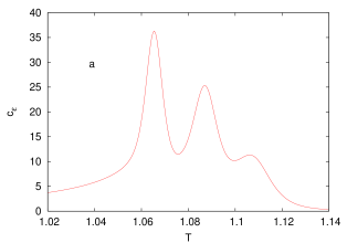
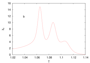
Plot of the order parameter $\theta$ as function of the temperature is represented in [Fig. 1], for a given sequence of length $N=2500$, and for sequences obtained by concatenating $t=2$ and $t=4$ times the original sequence. In the following [Fig. 2], we present data on the specific heat $c$ and the susceptibility $\chi$ for the same given sequence of length $N=2500$. We can observe in [Fig. 1] a clearly defined multi-step behaviour in the order parameter plot, with correspondingly three distinct peaks in the specific heat and in the susceptibility plots in [Fig. 2], even for this relatively short sequence considered.

We first notice, comparing the behaviours in [Fig. 2a] and [Fig. 2b], that the pseudo-critical temperature $T_{c}(\{\varepsilon_{i}\},N)$, defined as the temperature at which the susceptibility reaches its absolute maximum, is very close to the corresponding one obtained from the specific heat plot. This conclusion holds independently of the choice of a specific sequence. In fact, as already observed in [4], for the parameter values used (notably ratio $R=2$, between energies associated with $GC$ and $AT$ links), for each disordered configuration, the specific heat, the derivative with respect to temperature of the order parameter and the susceptibility always display very similar behaviours. In particular, as detailed below, it appears that the disorder averages of specific heat and of susceptibility (referring either to standard averages $\overline{(\cdot)}$ or to averages which take into account the sequence-dependent pseudo-critical temperature $\overline{\overline{(\cdot)}}$) display the same critical behaviour at $T_{c}$ and the same kind of finite size corrections to scaling.

Figure 1: Order parameter $\theta$ plotted as function of the temperature for a given sequence of length $N=2500$ and for the sequences of lengths $N=5000$ and $N=10000$ obtained by concatenating $t=2$, respectively $t=4$, copies of the original sequence.

Figure 2: a) Specific heat $c$; b) susceptibility $\chi$. Data are for the same given sequence of length $N=2500$ considered in the previous [Fig. 1], plotted as function of temperature.

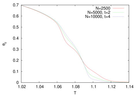
Interestingly, despite the multi-step behaviour, we observe in [Fig. 1] that the densities of closed base pairs $\theta(\{\varepsilon_{i}\},N,T)$, $\theta(\{\varepsilon_{i}\},2N,T)$ and $\theta(\{\varepsilon_{i}\},4N,T)$, respectively, cross at a well defined $T$-value, thus providing, following [5, 6], a different possibility for defining a pseudo-critical temperature $T_{c}^{\prime}(\{\varepsilon_{i}\},N)$, which we also study here. It appears reasonable to assume that the scaling properties of this observable should not depend on the particular way it is defined. However, to the best of our knowledge, there are no previous attempts for defining and studying in detail pseudo-critical temperatures in the presence of several distinct peaks in the specific heat or in the susceptibility and our definition of $T_{c}(\{\varepsilon_{i}\},N)$ as the position of the absolute maximum of the susceptibility appears reasonable in such case. In any event, in the present work, we checked that with our choice we get results compatible with those obtained with the alternative definition above, for chain lengths up to $N=2500$.

Figure 3: Susceptibility as function of temperature, plotted for independently randomly generated sequences of lengths $N=2500$, $N=5000$ and $N=10000$, respectively. The randomly generated sequence of length $N=2500$ is the same than the one used in the previous figures, hence the corresponding susceptibility is in particular the same than in [Fig. 2b].

Figure 4: Susceptibility as function of temperature, plotted for given sequences of lengths $N=2500$, $N=5000$ and $N=10000$, respectively. The randomly generated sequence of length $N=2500$ is the same in the two plots, corresponding to the one used in the previous figures, hence the corresponding susceptibility is in particular the same than in [Fig. 2b]. a) The sequence of length $N=5000$ coincides with the original sequence of length $N=2500$ for the first half, with the second half being randomly generated and, similarly, the sequence of length $N=10000$ coincides with the sequence of length $N=5000$ for the first half, with the second half being randomly generated; b) The sequences of length $N=5000$ and $N=10000$ correspond to the concatenation of $t=2$, respectively $t=4$, copies of the original sequence of length $N=2500$.

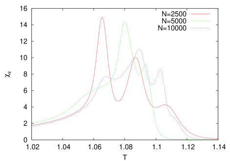
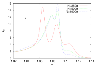
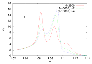
Moreover, checking the behaviour of the order parameters for sequences obtained by concatenation of $t$ copies of the original sequence, we can observe in [Fig. 1] that the multi-step behaviour becomes less evident for increasing chain lengths. To better understand the meaning of this observation, we consider, in [Fig. 3] and [Fig. 4], the evaluations of the susceptibility for different possible instances of sequences of increasing lengths, involving the original sequence of length $N=2500$, for which this observable displays three distinct peaks. In detail: in [Fig. 3] the sequences of lengths $N=5000$ and $N=10000$ are randomly generated, with accordingly no correlations between the three increasingly longer sequences; in [Fig. 4a], the sequences of length $2N$ correspond to the concatenation of the original sequence of length $N$ with a randomly generated sequence of length $N$; in [Fig. 4b] the sequences of length $tN$ correspond to the concatenation of $t$ instances of the original sequence of length $N$.

Most strikingly, in all these instances, increasing values for $N$ do not appear to be associated with the concomitant appearance of a larger number of peaks. Nevertheless, we can observe in these figures interesting qualitative differences between the three cases. In [Fig. 3], the behaviour of susceptibility for the longest sequences do not appear to be correlated with that of the shortest one, with notably such behaviour changing completely between $N=2500$ and $N=5000$ and the position of the absolute maximum for the sequence of length $N=5000$ corresponding to the position of a minimum for the sequence of length $N=2500$. On the contrary, in [Fig. 4], the presence of correlations between sequences of various lengths appear to be associated, not surprisingly, with concomitant correlations in the plots of the corresponding susceptibilities.

More specifically, it can be noticed in [Fig. 4] that in case a), which is the closest to the conditions of the Monte-Carlo like numerical studies on the disordered on-lattice SAW DNA model [34], significant correlations between susceptibility plots are observed for the longest sequences ($N=5000$ and $N=10000$), whereas in case b), which corresponds to the case of sequences generated by concatenations of a same original sequence, strong correlations between susceptibility plots are observed for all sequence lengths. In case b) it can be further noted that, with increasing chain lengths, the position of the absolute maximum for the susceptibility appears to approach the position for which crossing of the order parameters is observed in [Fig. 1].

As a matter of fact, the comparisons above highlight the importance of the protocols adopted for the generation of increasingly longer sequences. Moreover, in agreement with the picture proposed in [4], and as further detailed below, these comparisons also suggest the importance of the contribution of rare regions in the sequences to the thermodynamic limit behaviour of the disordered system considered. Indeed, in the concatenation scheme, as can be noticed notably in [Fig. 4b], the maximum length for such rare regions is strictly restricted by the maximum length of rare regions in the original sequence used.

4.2 The scaling behaviours of $T_{c}(N)$ and $\delta T_{c}(N)$

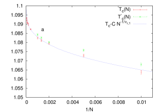
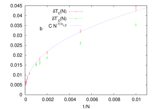
The values of $T_{c}(N)=\overline{T_{c}(\{\epsilon_{i}\},N)}$ and $\delta T_{c}(N)=\{\overline{[T_{c}(N)-T_{c}(\{\epsilon_{i}\},N)]^{2}}\}^{1/2}$, as functions of $1/N$, are plotted in [Fig. 5], along with the best fits obtained following $T_{c}(N)\propto T_{c}+C\>N^{-1/\nu_{r,1}}$ and $\delta T_{c}(N)\propto N^{-1/\nu_{r,2}}$, hence allowing the possibility, in principle, of two different exponents (see Eqs. (16)-(19) and the associated discussions). In addition, data for the mean value and for the fluctuations of $T_{c}^{\prime}(\{\epsilon_{i}\},N)$, defined according to [5, 6], are also plotted in [Fig. 5] for $N\leq 2500$. For each $N$-value, we also checked that the behaviour of $T_{c}(\{\epsilon_{i}\},N)$ agrees with a Gaussian distribution. We notice first of all that, interestingly, whereas strong finite size corrections are observed in the behaviour of average quantities when applying standard scaling laws [4], it appears that data on the mean value and on the fluctuations of the pseudo-critical temperature agree well with the corresponding expected laws on the whole $N$-range considered.

On such basis it is then straightforward to determine whether the values of the exponents are different, as associated to typical and average quantities, respectively. Indeed, it is immediately obvious from the figure that the data for $T_{c}(N)$ and $\delta T_{c}(N)$ (as the ones for $T^{\prime}_{c}(N)$ and $\delta T^{\prime}_{c}(N)$) display essentially the same $N$-dependence. This result implies that the pseudo first order transition scenario cannot describe the observed behaviour in the present case, since the mean value and the fluctuations of the pseudo-$T_{c}$ are ruled by the same exponent $\nu_{r}$ (which appears to be larger than $2$).

Figure 5: a) Plots of the mean values, $T_{c}(N)$ and $T_{c}^{\prime}(N)$, of the pseudo-critical temperatures as functions of $1/N$. $T_{c}(N)$ values are plotted for the various chain lengths (red marks with error bars), corresponding for a given $N$ to the mean value of $T_{c}(\{\epsilon_{i}\},N)$, associated with the temperature for which the susceptibility reaches its absolute maximum, for the various sequences. In addition, mean values of $T_{c}^{\prime}(\{\epsilon_{i}\},N)$ are plotted for $N\leq 2500$ (green marks with error bars), defined as the crossing points of the order parameters $\theta(\{\epsilon_{i}\},tN,T)$, for $t=1,2,4$. The dotted line corresponds to the best fit of $T_{c}(N)$, according to the scaling law $T_{c}(N)\simeq T_{c}+CN^{-1/\nu_{r,1}}$ (with $T_{c}=1.098\pm 0.001$ and $1/\nu_{r,1}=0.33\pm 0.03$). b) Plots of the fluctuations $\delta T_{c}(N)$ and $\delta T_{c}^{\prime}(N)$, associated with $T_{c}(N)$ and $T_{c}^{\prime}(N)$ in a), as functions of $1/N$. The dotted line corresponds to the best fit for $\delta T_{c}(N)$, according to the scaling law $\delta T_{c}(N)\propto N^{-1/\nu_{r,2}}$ (with $1/\nu_{r,2}=0.405\pm 0.01$).

$N_{0}$	$T_{c}$	$1/\nu_{r,1}$	$1/\nu_{r,2}$
100	1.098$\pm$0.001	0.33 $\pm$ 0.03	0.405 $\pm$ 0.01
200	1.101$\pm$0.002	0.27 $\pm$ 0.04	0.38 $\pm$ 0.01
500	1.101$\pm$0.003	0.27 $\pm$ 0.06	0.37 $\pm$ 0.01
750	1.099$\pm$0.003	0.32 $\pm$ 0.08	0.365 $\pm$ 0.01
1000	—	—	0.34 $\pm$ 0.02
2500	—	—	0.33 $\pm$ 0.06

Table 5: Estimations of $T_{c}$, $1/\nu_{r,1}$ and $1/\nu_{r,2}$ obtained disregarding chains of length $N<N_{0}$, for the different $N_{0}$ values considered. For $T_{c}$ and $1/\nu_{r,1}$ estimations are from $T_{c}(N)$ data, and for $1/\nu_{r,2}$ from $\delta T_{c}(N)$ data (see text).

For further deepened analysis, [Tab. 5] reports estimations of $T_{c}$ and $1/\nu_{r,1}$ (from $T_{c}(N)$), and of $1/\nu_{r,2}$ (from $\delta T_{c}(N)$), obtained disregarding chain lengths $N<N_{0}$, for different $N_{0}$ values. This analysis does not reveal any obvious finite size corrections to scaling in the behaviour of $T_{c}(N)$. On the other hand $1/\nu_{r,2}$ appears to display a weak dependence on $N_{0}$, decreasing to the value $1/\nu_{r,2}\sim 0.33\div 0.34$ when only chain lengths $N\geq 1000$ are considered. Thus we are led to similar values for the two exponents, with $1/\nu_{r,1}=1/\nu_{r,2}=1/\nu_{r}=0.35\pm 0.05$, and accordingly to the estimates: $\nu_{r}=2.9\pm 0.04$, and $c_{r}=1+1/\nu_{r}=1.35\pm 0.05$. It is moreover possible to notice that analysis of the mean value and of the fluctuations of $T_{c}^{\prime}(\{\epsilon_{i}\},N)$ leads to estimates ($1/\nu_{r,1}=0.44\pm 0.06$ and $1/\nu_{r,2}=0.38\pm 0.01$) which are consistent with the previous ones, even though in this case only chain lengths $N\leq 2500$ are considered.

Pseudo-critical temperatures appear thus to represent particularly interesting observables for the model here, with their scaling behaviour clearly in accordance with the typical scenario corresponding to relevance of disorder, the same than the one in the analysis of random ferromagnets [31, 33]: the numerical analysis provides evidence for a smooth phase transition (as already found in [4]), the thermodynamic limit behaviour being ruled by a single correlation length, in agreement notably with the mathematical findings in [1, 2, 3, 7]. More precisely, our present best estimation of the random critical point correlation length exponent ($\nu_{r}=2.9\pm 0.04$) is perfectly consistent with the previous evaluation in [4], obtained through the scaling of the maximum of the specific heat averaged over disorder in the standard way.

Importantly, it is also clear that, for the pseudo-critical temperature oriented analyses, asymptotic behaviours appear to be reached for chain lengths shorter than those considered in the present study (up to $N=2\cdot 10^{4}$), despite the strong finite size corrections to scaling characterizing the behaviour of the various thermodynamic observables in this disordered model [34, 4], This situation is expected to be related to the choice of parameters [4], and in order to reach a quantitative description of the dependency of the behaviour of the model on these parameters it would be relevant to determine a crossover chain length $N^{*}$, below which the present data could also agree with a pseudo first order transition.

With this respect, in order to grasp the behaviour of the model in the thermodynamic limit, looking in detail to [Fig. 5], it appears important on qualitative bases to have $N>1000$ (i.e. $1/N<0.001$). Indeed, with $N\leq 1000$, the average $T_{c}(\{\epsilon_{i}\},N)$, as a function of $1/N$, would appear instead to be adequately fitted with a straight line, while this is not true for $\delta T_{c}(\{\epsilon_{i}\},N)$. Thus the behaviour of these observables would be in agreement with a transition with $\nu_{r,2}>\nu_{r,1}=\nu_{p}=1$. Accordingly, $N^{*}\sim 1000$ can be retained as the evaluation of a crossover chain length suggested by data on the mean value and on the fluctuations of the pseudo-$T_{c}$ in our case. Clearly, such value corresponds to an evaluation from below, as the considered observables appear to be the less affected by corrections to scaling.

4.3 Comparisons between different ways of averaging

The behaviour of $\overline{\overline{\theta(\{\varepsilon_{i}\},T,N)}}$ is plotted in [Fig. 6], following the two definitions of pseudo-critical temperatures that we considered. Indeed, the present analysis aims to understand at a qualitative level the general results on quantities averaged by taking into account the pseudo-$T_{c}$ . With this respect the plots in [Fig. 6] can be compared to those presented in [4], in which the standard averaging method was used. In any case, we do not perform any finite size scaling analysis for the order parameter as, independent of the averaging method, the behaviour of this observable is not in agreement with the expected scaling law (hence with $N^{1-1/\nu_{r}}\tilde{\theta}[(T_{c}-T)N^{1/\nu_{r}}]$, with $\tilde{\theta}$ a scaling function, which can be derived from Eq. (20) with $e_{r}=\beta_{r}=\nu_{r}-1$). This feature was also observed both in [5] and in our previous work [4].

Figure 6: Plots of $\overline{\overline{\theta(\{\varepsilon_{i}\},N,T)}}$: a) the pseudo-critical temperature is defined as the value for which the absolute maximum of the susceptibility is reached; b) for chain lengths $N\leq 2500$, the pseudo-critical temperature is defined as the crossing point of the plots of $\theta(\{\varepsilon_{i}\},tN,T)$ (for $t=1,2$ and $4$, obtained from the concatenation of $t$ copies of the original sequence).

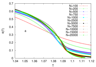
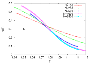
From a qualitative point of view, the data displayed in [Fig. 6] show unambiguously that, with varying $N$, the order parameters do not cross at the same temperature. This situation stands in sharp contrast with the one characterizing the pure model and also with the results reported in [5, 6]. As a matter of fact, this feature, clearly in disagreement with the possibility of a pseudo first order character for the behaviour of the model, was already observed in [4]. With the analyses here it further appears that this result do not dependent on the averaging method used. In fact, this result concerning crossovers becomes even more obvious for shorter chain lengths upon looking at the behaviour of $\overline{\overline{\theta}}$. Finally, this observation holds independently of the definition of the pseudo-critical temperature, even though the positions of the crossing points appear to vary in fact still more rapidly with $N$ when averaging is performed by taking the pseudo-$T_{c}$ as the abscissa of the absolute maximum of the susceptibility. Thus, the analysis in terms of pseudo-critical temperatures appears to reduce, in general, the importance of the finite size effects, hence allowing notably to extrapolate the correct thermodynamic limit behaviour from shorter chain lengths, (i.e. decreasing the effective $N^{*}$ value).

For further clarification, we finally consider in detail the behaviour of the average susceptibility, whose evaluation is expected to be the most sensitive to different ways of averaging. Indeed, notably in the context of the study here, resorting extensively to the definition of the pseudo-critical temperature as the position of the absolute maximum of susceptibility for a given sequence, the quantity ${\overline{\overline{\chi(\{\varepsilon_{i}\},T,N)}}}$ is expected to best highlight, with its possible divergence, a pseudo first character in the behaviour of the model (see Eq. (23)). Moreover, noticeably, the maximum of this quantity is expected to behave as a typical quantity, in the sense to be the observable the less affected by fluctuations in the pseudo-$T_{c}$ itself (see Eq. (23)). From this point of view the study of this quantity is also expected to best highlight possible differences between typical and average behaviours.

Figure 7: a) Plots of $\overline{\chi(\{\varepsilon_{i}\},T,N)}$ and ${\overline{\overline{\chi(\{\varepsilon_{i}\},T,N)}}}$ for chain length $N=2500$ as function of the temperature. b) Plots of the corresponding maxima as function of the system size. In the first case averaging is performed in the standard way (same data as in [4]). In the second case averaging is performed taking into account the pseudo-critical temperature, following the two definitions considered (i.e. with $T_{c}(\{\varepsilon_{i}\},N)$ the temperature where, for the given sequence, susceptibility reaches its absolute maximum and with $T_{c}^{\prime}(\{\varepsilon_{i}\},N)$ the temperature corresponding to the crossing point of the order parameter, for the given sequence, with those of the sequences obtained by concatenating variable number of copies of the given sequence).

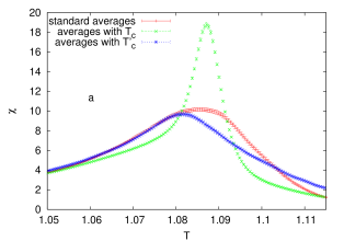
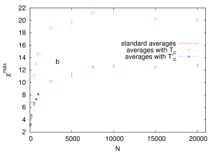
In detail, for the susceptibility data the results, for $N=2500$, are plotted in [Fig. 7a] for $\overline{\chi(\{\varepsilon_{i}\},T,N)}$ (as obtained from Eq. (11) and corresponding to the same data as in [4]) and for $\overline{\overline{\chi(\{\varepsilon_{i}\},T,N)}}$ (as obtained from Eq. (21)), using the two definitions of the pseudo-critical temperature ($T_{c}(\{\varepsilon_{i}\},N)$ and $T_{c}^{\prime}(\{\varepsilon_{i}\},N)$, respectively). It is then obvious from the figure that the possible pseudo first order character of the behaviour of the model is indeed suggested the most clearly by data on $\overline{\overline{\chi}}$ evaluated by defining the pseudo-$T_{c}$ as the abscissa of the absolute maximum of susceptibility (for a given sequence), i.e. $T_{c}(\{\varepsilon_{i}\},N)$, with the average susceptibility reaching a definitely highest maximum in this case. The observation is in agreement with the expected result, thereby confirming that the considered $T_{c}(\{\varepsilon_{i}\},N)$ is particularly appropriate for assessing disorder relevance. Moreover, in this context it becomes easy to determine the behaviour of the model with respect to the typical scenario.

In fact, when looking at the scaling behaviours of the maxima values as functions of $N$ in [Fig. 7b], a qualitative good agreement is found between the different ways considered for performing the averages. In particular, in all cases the maximum of the average susceptibility displays a crossing to an $N$-independent regime for the largest considered chain lengths, clearly showing that there is no difference in the behaviour of typical and average quantities. The data therefore further support a smooth transition (with $\gamma_{r}=\alpha_{r}\leq 0$, and accordingly $\nu_{r}=2-\alpha_{r}\geq 2$). From a different point of view, these findings also clearly confirm qualitatively that the thermodynamic limit behaviour of the model is described by a single correlation length, in agreement with the result following which the mean value and the fluctuations of the pseudo-$T_{c}$ scale with the same exponent (namely, $\nu_{r}=2.9\pm 0.4$). It is worth recalling that in our previous work [4], by fitting the data for the maximum of the specific heat (averaged in the standard way) to the law $C_{1}-C_{2}N^{\alpha_{r}/\nu_{r}}$, we obtained (with the first two points disregarded) $\alpha_{r}/\nu_{r}=-0.3\pm 0.1$, and hence $\nu_{r}=2.9\pm 0.6$. Hence, it would be meaningless to repeat the analysis on $\overline{\overline{\chi}}^{max}$ here.

Inasmuch as the data the data for $\overline{\max_{T}\{\chi(\{\varepsilon_{i}\},T,N)\}}$ display an abrupt change as function of $N$, it is all the more appropriate to introduce a crossover chain length $N^{*}$, for characterizing the slow approach of the model to the asymptotic regime. More precisely, we observe a shift from a short chain increasing behaviour to a long chain nearly constant one, around a value of $N^{*}\sim 2500$, which is compatible both with the estimate from below ($N^{*}\sim 1000$) obtained qualitatively from the scaling of the mean value and of the fluctuations of the pseudo-critical temperature and with the (more accurate) estimate from above ($N^{*}\sim 2.500\div 5.000$) obtained according to the behaviour of the loop-length probability distribution (see below).

4.4 Non self-averageness parameter related to susceptibility

As already recalled, both in the typical case of disorder relevance and within the pseudo first order transition scenario, one expects strong non self-averageness in the thermodynamic observables which are singular at the critical point. Accordingly, the parameter defined by Eq. (22), which measures the relative fluctuations of the observable averaged over disorder in the standard way, should display a constant behaviour instead of decreasing as a function of the system size $N$ at $T_{c}$. In fact, numerical evidence was reported in [6] for such a behaviour of the non self-averageness parameter related to $\overline{\theta}$, for the disordered PS models considered with different $c_{p}$ values, and notably for the one with $c_{p}=2.15$. It is therefore reasonable to assume that the same result should hold in the present system. Indeed, intuitively enough, since the single sequence order parameter displays multi-step behaviour in a significant fraction of the samples, the sequence-to-sequence fluctuations of this observable, averaged in the standard way, should play a role at least of the same importance than in the model studied with $c_{p}=2.15$ in [6], in which this behaviour is not observed.

Figure 8: Plots of the non self-averaging parameter related to susceptibility, ${\cal R}_{\chi}(N,T)$, as function of the temperature, for the different chain lengths considered. No accurate evaluations of the errors are performed, even though they are expected to be at most of the order of the observed oscillations of the quantity.

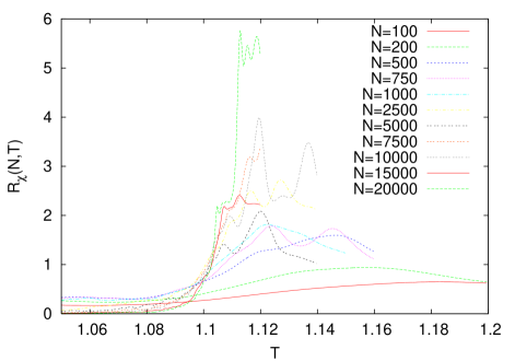
In this background, we instead focus here on the non self-averageness parameter related to the susceptibility, ${\cal R}_{\chi}(N,T)$, whose behaviour as function of $T$ is plotted in [Fig. 8], for the different sizes considered. First, letting aside the two shortest lengths $N=100$ and $N=200$, in the plots of ${\cal R}_{\chi}(N,T)$ no evident dependence on the chain length $N$ is observed for the heights of peaks, thus confirming the expected strong non self-averageness of this observable in the present model. The plots in [Fig. 8] display rather irregular behaviours in the whole high-$T$ region, even though it is in general expected that ${\cal R}\sim 1/N$ both above and below the critical point. This observation can be explained by the fact that here the disorder couples only to the low-temperature phase, with the order parameter being zero in the thermodynamic limit for $T>T_{c}$, where the two DNA strands are only linked at the origin. It is then particularly difficult to evaluate correctly in this region the fluctuations due to disorder of the average susceptibility.

Nevertheless, it is interesting to notice in [Fig. 8], that the plots for different $N$-values display similar behaviours near the thermodynamic limit critical temperature $T_{c}\simeq 1.1$. In particular, a steep increase is observed in the plots immediately above $T_{c}\simeq 1.1$, with the steepness increasing with the size, and for temperatures approaching $T_{c}$ from above for increasing sizes. In more quantitative terms, for the different $N$-values considered, the position of the highest ${\cal R}_{\chi}(N,T)$ peak, corresponding to the best evaluation of the abscissa of its absolute maximum as allowed by our present statistics, appears to be interpretable as the mean value of a quantity behaving as a pseudo critical temperature (or in any event as an $N$-depending evaluation of the thermodynamic limit critical temperature $T_{c}$), which we can denote $T^{\cal R}_{c}(N)$. In fact, we checked that the scaling law $T^{\cal R}_{c}(N)=T_{c}+CN^{-1/\nu_{r}}$ is also valid for this observable. With respect to the previous cases, corresponding to the two different definitions of $T_{c}(\{\varepsilon_{i}\},N)$, it is clear that the constant has the opposite sign, with anyway the fit leading to compatible estimations of $T_{c}$ and $\nu_{r}$.

5 Characterization of the finite size behaviour: results and insights

5.1 Crossover to the asymptotic regime

The quantity:

$$P^{\prime}(\{\varepsilon_{i}\},N,T,l)\equiv(2l)^{c_{p}}P(\{\varepsilon_{i}\},N,T,l),$$ (25)

was introduced in our previous work [4], as more appropriate for capturing relevance of disorder, than the loop-length probability distribution $P(\{\varepsilon_{i}\},N,T,l)$. Indeed, at the critical point, the logarithm of $P^{\prime}(\{\varepsilon_{i}\},N,T,l)$ is expected to be not constant and proportional to $(c_{p}-c_{r})\log l+C$ as soon as $c_{r}<c_{p}$.

In more detail, we can consider both $\log\overline{P^{\prime}(\{\varepsilon_{i}\},N,T,l)}$ and $\overline{\log P^{\prime}(\{\varepsilon_{i}\},N,T,l)}$, which should allow to capture the behaviours of the average and typical correlation lengths respectively, following the picture put forward in [5, 6] (with in fact the second case better described as a mixed average). The behaviour of these quantities for $T\simeq T_{c}$, as shown in [4], was instead found compatible with a smooth transition, but it is noticeable that the evaluated critical exponent $c_{r}$ appears to depend on $N$. In fact, such dependency is more evident when considering the average quantity $\overline{\log P^{\prime}(\{\varepsilon_{i}\},N,T_{c},l)}$, further displaying more important deviations from the expected behaviour ($\propto\log l$) than $\log\overline{P^{\prime}(\{\varepsilon_{i}\},N,T,l)}$.

In summary, the analysis of the data in [4] suggested the asymptotic condition $c_{r}<1.5$, which is confirmed by our present evaluation $c_{r}=1.35\pm 0.05$ obtained from the pseudo-$T_{c}$ behaviour. Nevertheless, to further clarify the situation, attempting to better characterize the finite size behaviour of the present model, we are led to study in detail both $\overline{\log P^{\prime}(\{\varepsilon_{i}\},N,T_{c},l)}$ and $\log\overline{P^{\prime}(\{\varepsilon_{i}\},N,T,l)}$ on the whole relevant $T$-range, by introducing effective ($N$-dependent) critical exponents $c_{r,1}(N)$ and $c_{r,2}(N)$, as well as correlation lengths $\xi_{1}(N,T)$ and $\xi_{2}(N,T)$.

We found that the data concerning $\log\overline{P^{\prime}(\{\varepsilon_{i}\},N,T,l)}$ are accurately described by the expected scaling law, which can be easily obtained from Eq. (9). Accordingly, the behaviour of $\log\overline{P^{\prime}(\{\varepsilon_{i}\},N,T,l)}$, which should be ruled by the fluctuations of the pseudo-$T_{c}$, is in agreement with:

$$\log\overline{P^{\prime}(\{\varepsilon_{i}\},N,T,l)}\simeq(c_{p}-c_{r,2}(N))\log l-l/\xi_{2}(N,T)+C(N).$$ (26)

On the other hand, in order to obtain a satisfactory fit (within the errors) for the data concerning $\overline{\log P^{\prime}(\{\varepsilon_{i}\},N,T,l)}$ (with such analysis expected to better capture the typical loop-length probability distribution behaviour), it appears necessary to introduce, in addition, a quadratic contribution in $l$, i.e.:

$$\overline{\log P^{\prime}(\{\varepsilon_{i}\},N,T,l)}\simeq(c_{p}-c_{r,1}(N))\log l-l/\xi_{1}(N,T)-C_{1}(N)l^{2}+C_{2}(N),$$ (27)

with the constant $C_{1}(N)$ tending towards zero roughly as $1/N$.

Such approach appears adequate to describe the strong finite size corrections to scaling characterizing the present model, and above all it allows a clear definition of $N^{*}$. In fact, the crossover between a short chain length regime in which the effective exponents would be in agreement with a pseudo first order transition and a long chain length one in which they would be compatible with the asymptotic values turns out to be quite abrupt. Therefore, one can obtain a quantitative evaluation of the crossover chain length (which is an evaluation from above), as the length $N^{*}$ beyond which $c_{r,1}(N)\sim c_{r,2}(N)\sim c_{r}\simeq 1.35$ and $\lim_{T\rightarrow T_{c}^{-}}\xi_{1}(N,T)\sim\lim_{T\rightarrow T_{c}^{-}}\xi_{2}(N,T)\sim(T_{c}-T)^{-\nu_{r}}$, with $1/\nu_{r}=c_{r}-1\simeq 0.35$.

Figure 9: a) Evaluation, for the various chain lengths considered, of $c_{p}-c_{r,2}(N)$ from the fits (three parameters) of $\log\overline{P^{\prime}(\{\varepsilon_{i}\},N,T,l)}$ to Eq. (26), as function of temperature. b) Evaluation, for the various chain lengths considered, of $c_{p}-c_{r,1}(N)$ from the fits (four parameters) of $\overline{\log P^{\prime}(\{\varepsilon_{i}\},N,T,l)}$ to Eq. (27), as function of temperature. For both analyses the errors are only of indicative value, as the results display some dependence on the $l$-range (with the range $l\in[3,N/3]$ considered corresponding to a reasonable choice), in particular for the shortest chain lengths. For comparisons, the expected asymptotic behaviour ($c_{p}-c_{r}\simeq 0.8$) is also represented in both panels.

Figure 10: a) Evaluation of the inverse of the correlation length as function of temperature for the various chain lengths considered, from the fits (three parameters) of $\log\overline{P^{\prime}(\{\varepsilon_{i}\},N,T,l)}$ to Eq. (26). b) Evaluation of the inverse of the correlation length $\xi_{1}(N,T)$ as function of temperature for the various chain lengths considered, from the fits (four parameters) of $\overline{\log P^{\prime}(\{\varepsilon_{i}\},N,T,l)}$ to Eq. (27). The same remarks as in [Fig. 9] apply to the significance of errors. For comparisons, the expected asymptotic behaviour ($1/\xi(T)\propto(T_{c}-T)^{2.9}$) is also represented in both panels.

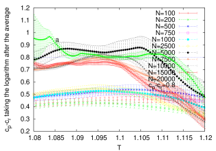
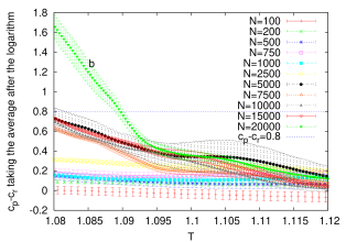
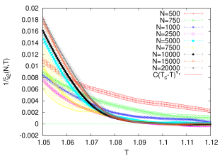
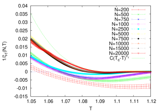
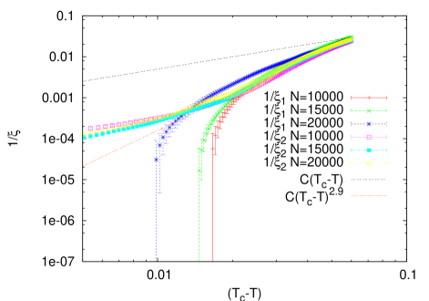
The detailed results for the loop-length probability distribution exponents and the inverse of the correlation lengths are presented in [Fig. 9] and [Fig. 10], respectively, associated with Eq. (26) and Eq. (27) in each of the two cases. More precisely, the figures plot the evaluations of $c_{p}-c_{r,2}(N)$, $c_{p}-c_{r,1}(N)$, $1/\xi_{1}(N,T)$ and $1/\xi_{2}(N,T)$, as obtained from the fits above, as functions of temperature for the different sizes considered. These plots also allow to compare the results with $c_{p}-c_{r}\simeq 0.8$ and $1/\xi(T)\sim(T_{c}-T)^{2.9}$ for $T\rightarrow T_{c}^{-}$ (the asymptotic inverse of the correlation length being zero in the whole high temperature phase).

The plots in [Fig. 9] and [Fig. 10] clearly illustrate the strong $N$-dependence of the quantities considered. Nonetheless, as shown in particular in [Fig. 9a], for chain lengths $N\geq 5000$, by allowing for a non-zero effective $1/\xi_{2}(N,T)$, $c_{p}-c_{r,2}(N)$ evaluations from $\log\overline{P^{\prime}(\{\varepsilon_{i}\},N,T,l)}$ are consistent with $c_{r}\simeq 1.35$ over a large temperature range around $T_{c}$. Accordingly, for the disordered PS model with $c_{p}=2.15$ studied, it appears that $N^{*}=2500\div 5000$ can be assimilated to our best evaluation from above of the crossover length $N^{*}$. This conclusion also holds for the analysis of $\overline{\log P^{\prime}(\{\varepsilon_{i}\},N,T,l)}$ data, even though involving in this case more significant corrections.

It is also very illustrative to notice that limiting the analysis to chain lengths $N<2500$ can lead to interpretations significantly different from those obtained considering the long chain length regime: one would get from [Fig. 9b] an estimate for $c_{p}-c_{r,1}(N)$ essentially compatible with the zero value characteristic of the pure case (i.e. $c_{r,1}=c_{p}=2.15$ which would imply $\nu_{r,1}=\nu_{p}=1$), as well as (from [Fig. 9a]) an estimate for $c_{r,2}(N)$ not significantly larger than 1.5 (i.e. $c_{r,2}=1+1/\nu_{r,2}$ with $\nu_{r,2}=2$). With this respect, the analysis here confirms, that in the regime below the crossover chain length $N^{*}$, it is difficult to extrapolate the correct thermodynamic limit behaviour on general grounds, with the results being indeed interpretable in such context according to the picture implying a pseudo first order phase transition as proposed in [5, 6].

Figure 11: Plots of $1/\xi_{2}(N,T)$ and $1/\xi_{1}(N,T)$ on log-log scale as functions of $(T_{c}-T)$ (with $T_{c}\simeq 1.1$) for the three longest chain lengths considered ($N=10000$, $N=15000$ and $N=20000$; same data as in [Fig. 10]). Data are plotted against the expected asymptotic behaviour of the inverse correlation length $1/\xi(T)\propto(T_{c}-T)^{\nu_{r}}$, with $T_{c}=1.1$ and $\nu_{r}=2.9$. For comparisons, the behaviour of $1/\xi(T)\propto(T_{c}-T)$ is also displayed.

Figure 12: a) Plots of $\log\overline{\overline{P^{\prime}(\{\varepsilon_{i}\},N,T_{c},l)}}$ as functions of $l$ at $T=T_{c}\simeq 1.1$, for the different chain lengths considered. b) Plots of $\overline{\overline{\log P^{\prime}(\{\varepsilon_{i}\},N,T_{c},l)}}$, as functions of $l$ at $T=T_{c}\simeq 1.1$, for the different chain lengths considered. For both a) and b) the averages are performed by taking into account the pseudo-critical temperature, following Eq. (21). All curves are shifted arbitrarily, setting them to zero for $l=2$. The expected asymptotic limit behaviour $\propto(c_{p}-c_{r})\log l+C$, with $c_{p}-c_{r}=0.8$ (i.e. $c_{r}=1.35$), is also plotted, in both panels, as a dotted line.

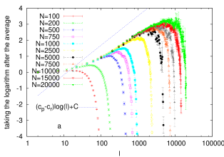
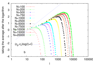
The importance of finite size effects is further highlighted in [Fig. 10]. This Figure allows to compare the behaviour of $1/\xi_{2}(N,T)$ ([Fig. 10a]; as obtained from Eq. (26)), with that of $1/\xi_{1}(N,T)$ ([Fig. 10b]; as obtained from Eq. (27)), with the plots clearly showing that the two quantities approach the asymptotic limit $\propto(T_{c}-T)^{\nu_{r}}$ with $\nu_{r}\simeq 2.9$ from opposite sides. In particular, for short chain lengths $N<N^{*}$, it appears that the value of $1/\xi_{2}(T,N)$ is definitely different from zero, on the whole $T$-range considered. It can be also observed that, in the same short chain length regime, for the average performed after taking the logarithm, negative (physically meaningless) values are obtained for $\xi_{1}(T,N)$ on a large part of the $T$-range (bearing in mind that in this case it appears necessary to insert also a quadratic term in $l$ in order to perform the data fit). Even though the data here do not allow a more quantitative analysis, these results further imply that below the crossover (i.e. for chain lengths $N<2500$) evidence is observed for the presence of two correlation lengths (and accordingly for two different critical exponents $\nu_{r,2}\neq\nu_{r,1}$).

On the other hand, the behaviours of $\xi_{1}$ and $\xi_{2}$ for $N>N^{*}$ are in agreement over a large $T$-range, within the error margins, with a correlation length exponent $\nu_{r}\simeq 2.9$, as clearly shown in [Fig. 11] displaying the plots of $1/\xi_{2}(N,T)$ and $1/\xi_{1}(N,T)$ for the three largest sizes considered. The fact that the two quantities converge towards the same behaviour is particularly meaningful: these observables are very demanding to be measured, and moreover they are the ones expected to be the most affected by corrections to scaling. Therefore, the result confirms that for $N\sim 10^{4}$ the asymptotic regime of the model considered is definitely reached.

Finally, for the different chain lengths, [Fig. 12] displays plots of $\log\overline{\overline{P^{\prime}(\{\varepsilon_{i}\},N,T_{c},l)}}$ and $\overline{\overline{\log P^{\prime}(\{\varepsilon_{i}\},N,T_{c},l)}}$ with the averages taking into account the pseudo-critical temperature, following Eq. (21). More precisely, in this case, for any given sequence, the loop-length probability distribution which contributes to the average is the one evaluated at the $T_{c}(\{\varepsilon_{i}\},N)$, where the susceptibility of the sequence reaches its absolute maximum. Upon comparing these plots to those of $\log{\overline{P^{\prime}(\{\varepsilon_{i}\},N,T_{c},l)}}$ and ${\overline{\log P^{\prime}(\{\varepsilon_{i}\},N,T_{c},l)}}$ in [4] (respectively [Fig. 6] and [Fig. 9], in this reference), it becomes once more clear that the analysis in terms of pseudo-critical temperatures allows to reduce the importance of finite size corrections to scaling. This can be seen first of all in the fact that here data corresponding to average after taking the logarithm display a behaviour more similar to the one in which the logarithm is taken after the average. Moreover both quantities approach qualitatively more rapidly the asymptotic behaviour $\propto(c_{p}-c_{r})\log l+C$, with $c_{r}\simeq 1.35$, in the present case.

5.2 Dependence of the crossover chain length on the model parameters

On general grounds, the rounding of the transition due to disorder in the present model should be mainly attributable to the presence of rare regions in the sequences (as expected in particular from the theoretical results [29]), or otherwise stated to the importance of the atypical events [1, 2, 3]. Accordingly, we attempt to quantify roughly their contribution in the finite size behaviour of the system, to better understand the way in which relevance of disorder becomes manifest, starting from the finite size level. This approach relies on the numerical evaluation here of $N^{*}$ for the particular model considered, as well as on the previously proposed very simplified phenomenological picture [4].

Qualitatively speaking, the approach is expected to be meaningful in the present case with $c_{p}>2$, corresponding to a first order transition in the pure model. Indeed, from the finite size behaviour point of view, this model appears to be characterized in general by a slow approach to the asymptotic regime, and the evidence for the effect of disorder (leading to the predicted smooth transition described by a single correlation length) appears to be related to the quite sudden appearance, at $N\sim N^{*}$, of enhanced (with respect to the $c_{p}\leq 2$ case) multi-step behaviours in the order parameter (and accordingly of different peaks in the susceptibility) in a significant fraction of the sequences considered. This feature can then be expected to be related to the presence in such sequences of large enough rare regions, which would then be already occurring, at $N\sim N^{*}$, with not negligible probability.

It is worth recalling that in [4] we showed notably that the relevant quantity from this point of view is expected to be the adimensional ratio between the rare region length $L$ (i.e. the number of consecutive base pairs of the same kind) and the value of the parameter:

$$x=\frac{R}{R-1}\frac{1}{\log\mu},$$ (28)

in the particular model à la PS with $c_{p}=2.15$ considered. This quantity is therefore to be interpreted as a measure of the effective disorder strength, linking the concept of large enough rare region to the values of $R=\varepsilon_{GC}/\varepsilon_{AT}$ and $\log\mu$ in the model.

Accordingly, we are led to the combinatorial problem of evaluating the probability ${\cal P}(N,L)$ to observe, in a sequence of total length $N$, a subsequence of consecutive base pairs of the same kind of length at least $L$. Such evaluation could appear to be rather simple. However even the obtention of the exact solution for the binomial quenched disordered variables distribution given by Eq. (3) appears to be far from trivial, and we resort here to the approximation:

$${\cal P}(N,L)\sim(N-L+1)\>2^{-L}.$$ (29)

This approximation is exact for $L=N$, but clearly invalid for small $L$ values, leading to probabilities higher than 1. Nonetheless, it can be considered that this approximation provides a reasonable basis for the present analysis, as we are mainly interested to capture the order of magnitude of the quantity (we checked numerically, by exact computations, that this is roughly the case, in a large $L$ range, already for small $N$ values).

As already outlined above, at the crossover it is expected to find large enough rare regions with a non-negligible probability. Here we set this probability to the value $0.5$, based on the observation that the order parameter displays multi-step behaviour at $N\sim N^{*}$ (i.e. multi-peak behaviour of the susceptibility) in a fraction of order $o(1)$ of the sequences considered. Accordingly, by applying Eq. (29) with ${\cal P}(N^{*},L^{*})=0.5$ (hence finding numerically the solution $L^{*}(N^{*})$ of $(N^{*}-L^{*}+1)2^{-L^{*}}=0.5$), we get an estimation of the crossover rare region length $L^{*}\sim 14$, in correspondence with the crossover chain length $N^{*}\sim 10^{3}\div 10^{4}$ which characterizes the present model. Assuming that the phenomenological picture does indeed capture the basic physics of the problem, and recalling that one has $x=x_{CY}\simeq 1.3$ in the present case, it is now in general easy to predict the behaviours of $L^{*}(x)$ and of the corresponding crossover chain length $N^{*}(x)$ as functions of the parameter $x$ in models à la PS for DNA denaturation transition with $c_{p}=2.15$. In fact, in order for the effect of disorder to be equally manifest in different models, it is expected to be necessary for the underlying ratio values $L^{*}(x)/x$ (of the crossover rare region length to the parameter $x$) to be similar [4]. Such conditions can be expressed as $L^{*}(x)=L^{*}(x_{CY})x/x_{CY}$. By using $x_{CY}=1.3$ with $L^{*}(x_{CY})=14$, it is then possible to obtain $N^{*}(x)$ by solving once again Eq. (29) with ${\cal P}(N^{*},L^{*})=0.5$.

In this way, for the PS model with $c_{p}=2.15$ in [5, 6], we find extremely large $N^{*}$ values of order $10^{30}\div 10^{50}$. Indeed, the link energies and the connectivity constant used in [5, 6] (which we recalled in [Tab. 3]) lead to $x=x_{GM}\simeq 16$. Taking also into account the somehow different law for the allowed coupling adopted in that study, the effective value of the parameter $x_{GM}$ is in fact expected to be still larger. Even though relying on rough evaluations, it appears therefore reasonable to consider that with the conditions in [5, 6] it would be impossible, in practice, to reach the asymptotic regime. In such context, the PS model with $c_{p}=2.15$ in [5, 6] is in fact indeed expected to behave in agreement with a pseudo first order transition, ruled by two correlation lengths (corresponding to typical and average quantities; namely with $\nu_{r,1}=\nu_{p}=1$ and $\nu_{r,2}=2$), independently from the observable considered and even well beyond the (already extremely large) chain lengths studied (up to $N=2\cdot 10^{6}$).

Thus, in the context of the analysis above, it appears possible to reconcile the two different pictures emerging from the previous numerical studies [34, 4, 5, 6]. Further, in such context, the scenario associated with the pseudo first order transition appears meaningful to describe the finite-$N$ behaviour in the presence of weak disorder. In this case, it would be moreover interesting to clarify the importance of boundary conditions, i.e. whether the second correlation length is better interpreted as the one related to the free-end distance or to an average loop length, with in fact the results here concerning the loop-length probability distribution favouring the second alternative.

Finally, it is worth noting that the $x_{CY}\simeq 1.3$ of the present model, which pertains to the region associated with large finite size effects (yet possible to study), is definitely closer to the still smaller $x_{exp}\simeq 0.2$ associated with the values of the coupling energies and of $\log\mu$ typically adopted for comparisons with experimental melting curves. In detail, the value of $R$ adopted for comparison with experiments is essentially the same ($R\simeq 1.1$) than the one in [5, 6], with, however, underlying link energies more than an order of magnitude smaller and a $\log\mu$ value more than an order of magnitude larger. The simple approximation of $P(L,N)$ considered may not be sufficient for precise predictions of $L^{*}_{exp}$ and $N^{*}_{exp}$ values. However, it seems reasonable to expect crossover rare region length of the order of a few base pairs, and a corresponding relatively small crossover chain length. From this point of view, the present results on the studied PS model with $c_{p}=2.15$ suggest that both self-avoidance and disorder could play a key role in experimental DNA behaviour.

Nevertheless, apart from the possible effect of neglecting correlations in the sequences, which are well known to be present in DNA molecules, a throughout understanding of this phenomenon would also require to better clarify the role of the cooperativity factor $\sigma_{0}$ in PS models. Indeed, in order to reproduce correctly the experimental curves, usually very small values, $\sigma_{0}\sim 10^{-4}\div 10^{-5}$, are adopted for this parameter (see in particular [49]). It would be also meaningful to further characterize the influence of this parameter, of non-universal character, on the finite size behaviour of the system (corresponding roughly to the introduction of an additional correlation length $\xi_{\sigma_{0}}\sim 1/\sigma_{0}$).

6 Conclusions

We performed an extensive numerical analysis of a disordered PS model with $c_{p}=2.15$, hence with the loop-length probability distribution exponent of the pure system taking completely into account self-avoidance. The analyses are following two main directions: i) a finite size scaling study in terms of appropriately defined pseudo-critical temperatures and ii) an attempt to characterize the peculiar finite size behaviour of the model.

Completing previous numerical results [34, 4], and in agreement with the predictions based on a probabilistic mathematical approach [1, 2, 3, 7], the present work notably provides evidence that the thermodynamic limit behaviour of the model is coherent with the picture describing random ferromagnets [33, 31]: a smooth transition described by a single correlation length (with the refined estimation here for the corresponding critical exponent $\nu_{r}=2.9\pm 0.4$).

The pseudo-critical temperature itself, that we define for taking appropriately into account the possible presence of multiple steps in the order parameter for a given sequence (checking its compatibility with a different definition suggested in [5, 6] for the same model) appears to be a particularly interesting observable to study. In detail, we find that the mean value and the fluctuations of this pseudo-critical temperature agree well with the expected scaling laws in the typical scenario corresponding to disorder relevance. And accordingly, the two quantities appear to be ruled by the same critical exponent (the one corresponding to the correlation length), on the whole $N$-range considered, without displaying the strong corrections to scaling observed in other quantities.

On this basis, it is also interesting to notice that the refined estimation of $\nu_{r}$ obtained with this analysis is further compatible with the estimation $\nu_{r}\simeq 2.7$ given in [6], for a PS model with the different $c_{p}=1.75$. Therefore, the results here could also support the hypothesis that the random PS model critical behaviour is independent on the $c_{p}$ value, as soon as the pure PS model undergoes a transition characterized by a diverging specific heat.

From this point of view, it can be nevertheless noticed that we focused here on the simplest possible scaling picture, therefore that the present study does not rule out the possibility that the complete description of the random system could involve more than a single independent critical exponent. In such case, it could be possible to get a scaling law obeyed by the order parameter and a better scaling of the loop-length probability distribution at $T\neq T_{c}$. However such possibility, whose exploration would represent a new subject, would clearly not impact the present result on $\nu_{r}$, and it is not expected to impact neither the present results on the characterization of the finite size behaviour.

Moreover, in any event, the observation that in the present model the order parameter behaves as the energy, and the susceptibility as the specific heat, could be relevant only for the disordered regime considered. More specifically, we did not investigate here the strong disorder regime of the model. Indeed, for $\varepsilon_{GC}>>\varepsilon_{AT}$, the observed behaviour could be more complex, since models à la PS are expected to display an additional singularity of the Kosterlitz-Thouless kind [50, 51, 52].

The present analysis also shows qualitatively that the finite size corrections are in general smaller when quantities are averaged taking into account the pseudo-critical temperatures. Finally, based on the study of an appropriately defined non self-averageness parameter, evidence is provided that the susceptibility is a strongly non self-averaging quantity at the critical point, with its detailed behaviour further allowing to get an alternative evaluation of both $T_{c}$ and $\nu_{r}$, compatible with our previous ones.

In this background, mainly in the second part of the work, we seek a better understanding of finite size effects. The data for the maximum of the susceptibility, and even more so the detailed study of the behaviour of the loop-length probability distribution, give weight to the existence of a crossover chain length $N^{*}$ below which one could not rule out the picture proposed in [5, 6]. This alternative scenario, the pseudo first order phase transition one, is indeed found to capture the behaviour of a different PS model with the same $c_{p}=2.15$ up to the extremely large sizes of $N=2\cdot 10^{6}$. In detail, we present a qualitative evaluation from below of $N^{*}\geq 1000$ from data on the pseudo-$T_{c}$, and a more quantitative evaluation from above of $N^{*}\leq 2500\div 5000$ from data on the loop-length probability distribution.

We also provide a tentative quantification of the dependence of $N^{*}$ on the parameters of the model, with notably an evaluation of the crossover length behaviour which could allow to reconcile the results here with those in [5, 6]: with the parameters chosen for the model in [5, 6] it could be not possible to reach the asymptotic regime in practice. In this context, we also find that the crossover chain length obtained for realistic parameter values (as used in experimental settings) should be definitely smaller than the present $N^{*}$ and, accordingly, our conclusions, concerning both the importance of self-avoidance and the relevance of disorder, should be also important for better modeling experimental DNA denaturation.

It is finally also interesting to stress that these extensive studies of the finite size behaviour, particularly in the case of PS models for DNA denaturation transitions, were made possible thanks to the recursive equations for the partition functions (notably within the SIMEX scheme), reducing essentially the time complexity of the problem to $\ln(N)N$.

In conclusion, it is possible that crossover effects, such as those described here, could be relevant in a larger class of disordered systems (at least in the behaviour of certain observables), allowing a better understanding of the finite size behaviour, and in particular of the way in which relevance of disorder becomes manifest when approaching the thermodynamic limit. In this sense the results and treatments here could provide interesting insights for the exploration of such disordered systems, on more general grounds. On the biological side, the results here should also contribute to a better understanding of the roles played by disorder and self-avoidance in experimental DNA denaturation, with notably a quantitative description of the finite size effect particularly important in this context.

References

- [1] G. Giacomin and F.L. Toninelli, Smoothing of depinning transitions for directed polymers with quenched disorder, 2006, Phys. Rev. Lett. 96, 060702.
- [2] G. Giacomin and F.L. Toninelli, Smoothing effect of quenched disorder on polymer depinning transitions, 2006, Commun. Math. Phys. 266, 1.
- [3] G. Giacomin, Random Polymer Models, 2007 (Imperial College Press, London).
- [4] B. Coluzzi and E. Yeramian, Numerical evidence for relevance of disorder in a Poland-Scheraga DNA denaturation model with self-avoidance: scaling behavior of average quantities, 2007, Eur. Phys. J. B 56, 349.
- [5] T. Garel and C. Monthus, Numerical study of the disordered Poland–Scheraga model of DNA denaturation, 2005 J. Stat. Mech., P06004.
- [6] C. Monthus and T. Garel, Distribution of pseudo-critical temperatures and lack of self-averaging in disordered Poland-Scheraga models with different loop exponents, 2005, Eur. Phys. J. B 48, 393.
- [7] F.L. Toninelli, Correlation lengths for random polymer models and for some renewal sequences, 2007, Electron. J. Probab. 12, 613.
- [8] D. Poland and H.A. Scheraga, Phase transitions in one dimension and the helix—coil transition in polyamino acids, 1966, J. Chem. Phys. 45, 1456; Occurrence of a phase transition in nucleic acid models, 1966, J. Chem. Phys. 45, 1464;
- [9] D. Poland and H.A. Scheraga (eds.), Theory of Helix-Coil Transitions in Biopolymers, 1970, (Academic, New York).
- [10] M.E. Fisher, Effect of excluded volume on phase transitions in biopolymers, 1966, J. Chem Phys. 45, 1469.
- [11] R.M. Wartell and A.S. Benight, Thermal denaturation of DNA molecules: A comparison of theory with experiment, 1985, Phys. Rep. 126, 67.
- [12] R.D. Blake, et al., Statistical mechanical simulation of polymeric DNA melting with MELTSIM, 1999, Bioinformatics, 15, 370.
- [13] D. Jost and R. Everaers, A unified Poland-Scheraga model of oligo- and polynucleotide DNA melting: salt effects and predictive power, 2009, Biophys. J. 96, 1056.
- [14] E. Yeramian, Genes and the physics of the DNA double-helix, 2000, Gene 255, 139; The physics of DNA and the annotation of the Plasmodium falciparum genome, 2000, Gene 255, 151.
- [15] E. Yeramian and L. Jones, GeneFizz: a web tool to compare genetic (coding/non-coding) and physical (helix/coil) segmentations of DNA sequences. Gene discovery and evolutionary perspectives, 2003, Nucl. Acid Res. 31, 3843.
- [16] E. Yeramian, S. Bonnefoy and G. Langsley, Physics-based gene identification: proof of concept for Plasmodium falciparum, 2002, Bioinformatics 18, 190.
- [17] E. Carlon, M.L. Malki and R. Blossey, Exons, Introns, and DNA Thermodynamics, 2005, Phys. Rev. Lett. 94, 178101.
- [18] M.E. Fisher, Walks, walls, wetting, and melting, 1984, J. Stat. Phys. 34, 667.
- [19] Y. Kafri, D. Mukamel and L. Peliti, Why is the DNA Denaturation Transition First Order?, 2000, Phys. Rev. Lett. 85, 4988. A. Hanke and R. Metzler, Comment, 2003, Phys. Rev. Lett. 90, 159801; Y. Kafri, D. Mukamel and L. Peliti, Reply, 2003, Phys. Rev. Lett. 90 159802.
- [20] Y. Kafri, D. Mukamel and L. Peliti, Melting and unzipping of DNA, 2002, Eur. Phys. J. B 27, 135.
- [21] B. Duplantier, Polymer Network of fixed topology: renormalization, exact critical exponent in two dimensions, and , 1986, Phys. Rev. Lett. 57, 941; Statistical mechanics of polymer networks of any topology, 1989, J. Stat. Phys. 54, 581.
- [22] M. S. Causo, B. Coluzzi and P. Grassberger, Simple model for the DNA denaturation transition, 2000, Phys. Rev. E 62, 3958.
- [23] E. Carlon, E. Orlandini and A.L. Stella, Roles of stiffness and excluded volume in DNA denaturation, 2002, Phys. Rev. Lett. 88, 198101.
- [24] M. Baiesi, E. Carlon and A.L. Stella, Scaling in DNA unzipping models: Denaturated loops and end segments as branches of a block copolymer network, 2002, Phys. Rev. E, 66, 021804.
- [25] M. Baiesi, et al., Interstrand distance distribution of DNA near melting, 2003, Phys. Rev. E, 67, 021911.
- [26] H. Kunz and R. Livi, DNA denaturation and wetting in the presence of disorder, 2012, Europhys. Lett. 99, 30001.
- [27] A.B. Harris, Effect of random defects on the critical behaviour of Ising models, 1974, J. Phys. C 7, 1671.
- [28] J.T. Chayes, L. Chayes, D.S. Fisher and T. Spencer, Finite-size scaling and correlation lengths for disordered systems, 1986, Phys. Rev. Lett. 57, 2999.
- [29] M. Aizenman and J. Wehr, Rounding of first-order phase transitions in systems with quenched disorder, 1989, Phys. Rev. Lett. 62, 2503; Erratum, 1990, Phys. Rev. Lett. 64, 1311.
- [30] A.N. Berker, Critical behavior induced by quenched disorder, 1993, Physica A 194, 72.
- [31] A. Aharony and A.B. Harris, Absence of Self-Averaging and Universal Fluctuations in Random Systems near Critical Points, 1996, Phys. Rev. Lett. 77, 3700.
- [32] R. Brout, Statistical Mechanical Theory of a Random Ferromagnetic System, 1959, Phys. Rev. 115, 824.
- [33] S. Wiseman and E. Domany, Finite-Size Scaling and Lack of Self-Averaging in Critical Disordered Systems, 1998, Phys. Rev. Lett. 81, 22; Self-averaging, distribution of pseudocritical temperatures, and finite size scaling in critical disordered systems, 1998, Phys. Rev. E 58, 2938.
- [34] B. Coluzzi, Numerical study of a disordered model for DNA denaturation transition, 2006, Phys. Rev. E, 73 011911.
- [35] M.N. Barber, Finite Size Scaling, in Phase Transitions and Critical Phenomena, Vol. 8, 1983, edited by C. Domb and J.L. Lebowitz (Academic, New York).
- [36] W. Selke, L.N. Shchur, and A.L. Talapov, Monte Carlo Simulations of Dilute Ising Models, in Annual Reviews of Computational Physics, 1994, edited by D. Stauffer (World Scientific, Singapore).
- [37] K. Binder and P. Young, Spin glasses: Experimental facts, theoretical concepts, and open questions, 1986, Rev. Mod. Phys. 58, 801.
- [38] J. Zinn-Justin, Quantum Field Theory and Critical Phenomena, Fourth Edition, 2002 (Clarendon Press, Oxford).
- [39] D.S. Fisher, Random transverse field Ising spin chains, 1992 Phys. Rev. Lett. 69, 534; Critical behavior of random transverse-field Ising spin chains, 1995, Phys. Rev. B 51, 6411.
- [40] F. Iglói, Yu-Cheng Lin, H. Rieger, C. Monthus, Finite-size scaling of pseudocritical point distributions in the random transverse-field Ising chain, 2007, Phys. Rev. B 76, 064421.
- [41] C. Monthus and T. Garel, Random wetting transition on the Cayley tree: a disordered first-order transition with two correlation length exponents, 2009, J. Phys. A: Math. Theor. 42, 165003.
- [42] A. Billoire, et al, Finite size scaling analysis of the distribution of critical temperatures in spin glasses, 2011, J. Stat. Mech., P10019.
- [43] M. Fixman and J.J. Freire, Theory of DNA melting curves, 1977, Biopolymers 16, 2693.
- [44] E. Yeramian, et al., An optimal formulation of the matrix method in statistical mechanics of one-dimensional interacting units: Efficient iterative algorithmic procedures, 1990, Biopolymers 30, 481.
- [45] E. Yeramian, Complexity and tractability. Statistical mechanics of helix-coil transitions in circular DNA as a model-problem, 1994, Europhys. Lett. 25, 49.
- [46] E. Yeramian and P. Claverie, Analysis of multiexponential functions without a hypothesis as to the number of components, 1987, Nature 326, 169.
- [47] P. Claverie, A. Denis and E. Yeramian, The representation of functions through the combined use of integral transforms and Padé approximants: Padé-Laplace analysis of functions as sums of exponential, 1989, Comput. Phys. Rep. 9, 247.
- [48] E. Yeramian and E. Debonneuil, Probabilistic sequence alignments: Realistic models with efficient algorithms, 2007, Phys. Rev. Lett. 98, 078101.
- [49] R. Blossey and E. Carlon, Reparametrizing the loop entropy weights: Effect on DNA melting curves, 2003, Phys. Rev. E 68, 061911.
- [50] L.-H. Tang and H. Chaté, Rare-event induced binding transition of heteropolymers, 2001, Phys. Rev. Lett. 86, 830.
- [51] Y. Kafri and D. Mukamel, Griffiths singularities in unbinding of strongly disordered polymers, 2003, Phys. Rev. Lett. 91, 055502.
- [52] B. Derrida and M. Retaux, The depinning transition in presence of disorder: A toy model, 2014, J. Stat. Phys. 156, 268.