On Weak Lensing Shape Noise

Abstract

One of the most powerful techniques to study the dark sector of the Universe is weak gravitational lensing. In practice, to infer the reduced shear, weak lensing measures galaxy shapes, which are the consequence of both the intrinsic ellipticity of the sources and of the integrated gravitational lensing effect along the line of sight. Hence, a very large number of galaxies is required in order to average over their individual properties and to isolate the weak lensing cosmic shear signal. If this ‘shape noise’ can be reduced, significant advances in the power of a weak lensing surveys can be expected. This paper describes a general method for extracting the probability distributions of parameters from catalogues of data using Voronoi cells, which has several applications, and has synergies with Bayesian Hierarchical modelling approaches. This allows us to construct a probability distribution for the variance of the intrinsic ellipticity as a function of galaxy property using only photometric data, allowing a reduction of shape noise. As a proof of concept the method is applied to the CFHTLenS survey data. We use this approach to investigate trends of galaxy properties in the data and apply this to the case of weak lensing power spectra.

1 Introduction

Advances in observational cosmology in the last two decades have indicated that the expansion of the Universe is accelerating (e.g. Riess et al., 1998; Perlmutter et al., 1999; Schrabback et al., 2010; Komatsu et al., 2011; Bennett et al., 2013; Planck Collaboration et al., 2014a, b; Planck Collaboration, 2015), rather than decelerating, as previously expected. Consequently, new models have been proposed as revisions to our current cosmological model (for a review see e.g. Amendola et al. (2013); Clifton et al. (2012)), ranging from revisions of general relativity to the existence of a non-zero vacuum energy, generically termed “dark energy”, to a revision in the fundamental large-scale assumptions for the Universe (such as isotropy and homogeneity, for papers discussing relaxing the assumption of isotropy, see e.g. Jaffe et al. (2005); McEwen et al. (2013); Planck Collaboration et al. (2014c, 2015)). Methodologies such as weak lensing and galaxy clustering are being developed to place observational constraints on these different approaches, and are becoming increasingly powerful, as they are explored and their characteristics and statistical behaviours understood.

One of the most powerful techniques currently available is weak gravitational lensing (see e.g. Kaiser, 1992; Bartelmann & Schneider, 2001; Albrecht et al., 2006; Peacock et al., 2006; Hoekstra & Jain, 2008; Munshi et al., 2008; Massey et al., 2010; Weinberg et al., 2013, and references therein). Through its gravitational effect, matter acts on light rays from a source to observer, and hence distorts the observed shape of the source; in analogy to an optical lens. Away from large concentrations of matter, such as the centre of galaxy clusters, this effect is very small: a change in the observed third flattening, or third eccentricity (colloquially referred to as ‘ellipticity’) of an image of a galaxy of only a few percent, an effect known as weak lensing. However if large enough samples of galaxies are observed, with sufficient attention to observational systematics, then a statistical analysis of the ensemble can be used to infer the matter distribution along the line of sight. Sources at higher redshift allow the mapping of the matter distribution at earlier times, and from the growth of structure and the relation of the amount of distortion to the expansion history of the Universe, inferences can be made on cosmological parameters (e.g. Semboloni et al., 2006; Kitching et al., 2007; Benjamin et al., 2007; Fu et al., 2008; Schrabback et al., 2010; Kilbinger et al., 2013; Kitching et al., 2014).

The change in the ellipticity of galaxies resulting from the gravitational lensing effect is known as ‘shear’. Ellipticity is an unbiased shear estimator, however galaxies are also intrinsically (in the absence of lensing) elliptical. However the orientation angle of the intrinsic ellipticity is expected to be randomly distributed on large scales, which allows one to recover the shear by averaging over many galaxies. In more detail, because galaxies to a first approximation have a random projected orientation on the sky the intrinsic ellipticity acts as an additional noise term when attempting to measure the shear of an object: the observed ellipticity is a sum of shear and intrinsic ellipticity $e=e^{\rm int}+g$, where $g$ is known as the reduced shear. The variance on the observed ellipticity is $\sigma^{2}(e)=\sigma^{2}(e^{\rm int})+\sigma^{2}(g)$. The variance of the intrinsic ellipticity is the dominant term, typically by a factor exceeding an order of magnitude. Hence, a very large number of galaxies are required in order to reduce this by averaging over their individual properties and to isolate the weak lensing signal. This term is commonly referred to as “shape noise”, and it is by far the largest source of uncertainty in weak lensing measurements. Shape noise is a limiting fundamental noise source in weak lensing measurements that determines the size of the observational surveys being designed to measure cosmological parameters using weak lensing: future state-of-the-art surveys such as that to be carried out by the European Space Agency’s Euclid mission (for details, see Laureijs et al., 2011, 2012; Amendola et al., 2013, and http://www.euclid-ec.org/) encompass most of the extragalactic sky. It follows, therefore, if this source of noise could be reduced, significant advances in the power of a weak lensing survey would follow, or smaller and less ambitious surveys could be contemplated while maintaining the previous survey sensitivity.

Recently Huff et al. (2013) have noted that the Tully-Fisher relationship could in principle be used as a proxy for the intrinsic ellipticity of a galaxy. However Tully-Fisher analyses are not practicable in a weak lensing context owing to the very large number of galaxies required, most of which are faint and hence have a low signal-to-noise ratio. Here we propose to generalise the concept to allow the incorporation of any other supplementary useful information that will provide prior knowledge on the intrinsic ellipticities, and which would be practicable. This could be any measurable property of a galaxy that does not have a correlation with shear. In this paper we use as an example the optical magnitudes of the galaxies and their combination (pseudo-colours), in the expectation that certain galaxy types (characterised by certain colours) have a range of ellipticity which is different from other galaxy types (characterised by different colours) (for a related study with COSMOS sample and the Millennium Simulation, in the context of intrinsic galaxy alignments, see Joachimi et al., 2013).

What we propose is a general method to infer the probability distribution of the intrinsic galaxy ellipticity $p(|e|)$ from a weak lensing ellipticity catalogue, in particular how to characterise the variance of this distribution. We also show how the probability of this distribution can be accessed, as this is particularly useful in the context of Bayesian hierarchical modelling (e.g. Schneider et al., 2014). Currently a Gaussian probability distribution for $p(e_{i})$ is assumed, with a mean for the two ellipticity components $(i)$ of zero and a standard deviation $\sigma(e_{i})$. This standard deviation can be derived from an observed $p(|e|)$ from a calibration set (for example from higher spatial resolution subsets of the data), or it can be taken from the dispersion in the measurement of the ellipticities of the galaxies. If the ellipticity measurement is carried out using a model-fitting method, for example lensfit (Miller et al., 2007), the ellipticity distribution $p(|e|)$ also acts as prior, which again may be from a calibration set of higher resolution; as used in, for example the CFHTLenS analysis (Miller et al., 2013).

The structure of this paper is as follows. In Section 2 we describe the data used and our methodology, and then in Section 3 we show how the limitation of the resulting $p(|e|)$ ellipticity dispersion width $\sigma(|e|)$ can be used to more optimally weight the dataset to achieve increased dark energy Figure of Merit (FoM) (Albrecht et al., 2006). Finally, we summarise and conclude in Section 4.

2 Data and Methodology

In this Section we present our general methodology. The central concept is that using clustering analysis (where the proximity of data points as a function of input features is estimated) of catalogue data the functional dependency of the variance of parameters of interest (in our case ellipticity of galaxies) on those parameters can be inferred. These approaches in fact already have a far more general application than that which we propose here, we are simply applying existing machine learning methodologies in a novel cosmological context. We first describe the data that we will use to develop the example of this paper, before describing the general algorithm, and then the specifics of the example implementation.

2.1 Data

The data we use are from the CFHTLenS (see e.g. Heymans et al., 2012) catalogue (Erben et al., 2013), which is a measurement of galaxy ellipticities (using the lensfit method by Miller et al. (2007)), galaxy photometric redshifts [Hildebrandt et al. (2012), using BPZ (e.g. Benítez, 2000; Coe et al., 2006)] and also includes in the catalogue derived meta-parameters such as galaxy stellar mass and bulge-to-disc ratio. The total data set corresponds to observations in five optical bands, ugriz, over $154$ square degrees of sky. We use the catalogues downloaded from http://www.cadc-ccda.hia-iha.nrc-cnrc.gc.ca/community/CFHTLens/query.html, and make no cuts in the catalogue.

2.2 Algorithm Overview

The algorithm, expanded upon in detail in the following sections, is in general terms the following. We assume that there are some parameters of interest (in our case ellipticity), and some meta-parameters that may (or may not) be related to the parameters of interest. The objective is to determine how the probability distribution of the parameters of interest is a function of the meta-parameters. Using a typical catalogue the dependency of the mean of the parameters is trivial to determine, but the full probability distribution is not.

In summary, we adopt the following approach:

1. First we perform a dimensionality reduction on the data. This can be of any form, but is required to remove degeneracies and to enable computationally efficient subsequent steps. In our example we use principal component analysis (PCA; Pearson, 1901), but this could be generalised for example to manifold learning (e.g. locally-linear embedding, isomap, etc.; Bengio et al. (2012)) or auto-node mapping (where the input is linked to the output nodes) in neural net analysis. At this stage a removal of the covariance of the parameters is also beneficial.

2. Next we perform a clustering analysis on the resulting parameters. This clustering analysis should be designed to find points in the parameters that are ‘close’ in some pre-defined distance measure (the most straightforward being the geometric distance between the points in the parameter space, but more general measures can be envisioned).

3. Finally the statistical properties in each cluster cell, labelled by a combination of meta-parameters, of the parameters of interest can now be computed. For example, this could be the mean and standard deviation, amongst other statistics. Furthermore, probability density functions can also be derived using, for example, kernel density estimation (see e.g. Rosenblatt, 1956; Parzen, 1962; Rudemo, 1982; Cao et al., 1994).

We now specify the details of the implementation of this approach that we take as an example in this paper, and apply this methodology to the CFHTLenS catalogue. We then apply this methodology to the case of reducing the shape noise term in weak lensing power spectrum analysis in an effort to increase the accuracy on the measurement of cosmological parameters for weak lensing analysis.

2.3 Dimensionality Reduction

Our chosen technique relies on identifying relations between photometric data and ellipticity measurements. The clarity of these relationships will be more evident if we project the five dimensional space of the CFHTLenS photometry (from the five bands) to a lower-dimensional surface within it which captures most of the information content. Our motivation for dimensionality reduction is to find those directions in the data that contain the majority of the information on the correlation (of more general relationship) between variables. Hence we perform a dimensionality reduction using PCA (Pearson, 1901), which uses an orthogonal transformation to convert a set of observations of possibly correlated variables into a set of values of maximally linearly uncorrelated orthogonal variables called principal components. Before performing the dimensionality reduction with PCA we whiten the data allowing to project the data onto the singular space while scaling each component to unit variance. This is useful because the clustering algorithm we adopt below makes assumptions on the isotropy of the signal. In the analyses we use the RandomizedPCA (Halko et al., 2009) implementation of the Scikit Learn package (Pedregosa et al., 2011). In this process, the linear combinations of magnitudes effectively produces a colour-colour hyperspace.

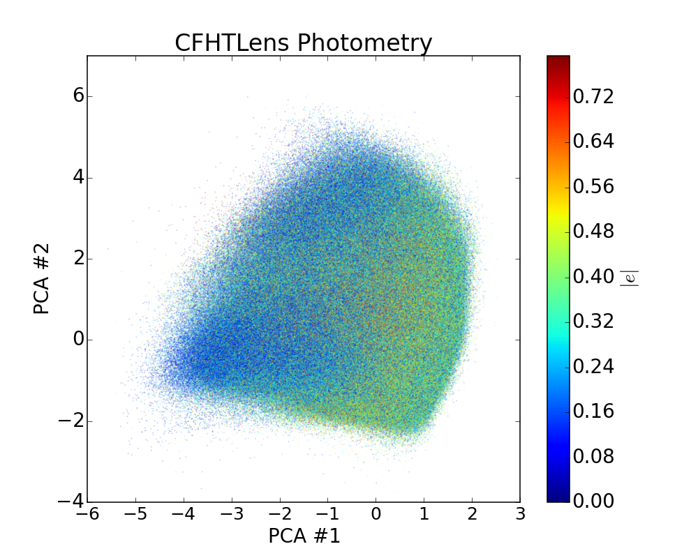
Figure 1 shows the CFHTLenS photometry projected onto the two dimensions with the highest eigenvalue principal components. Jointly the two first principal components explain approximately $96$ per cent of the variance in the original CFHTLenS photometry. The PCA components with the two highest eigenvalues are the following:

$$\left(\begin{array}[]{rrrrr}0.20&0.22&0.25&0.25&0.25\\ 0.96&0.49&-0.08&-0.45&-0.67\\ \end{array}\right)\left(\begin{array}[]{c}u\\ g\\ r\\ i\\ z\\ \end{array}\right)\,.$$ (1)

Thus, PCA#1 can be interpreted to represent an averaged broad band (‘white light’) magnitude, while PCA#2 amounts to a colour term ‘blue $-$ red’, where the blue part is a combination of $u$ and $g$ and the red is comprised mostly of $i$ and $z$.

In Figure 1, we colour-code each of the $5770490$ galaxies with the modulus of their ellipticity $|e|$, calculated from the ellipticity components $e_{i}$ as $|e|=\sqrt{e_{1}^{2}+e_{2}^{2}}$, measured in the CFHTLenS survey. Regions with lower mean ellipticity, broadly, those with negative values in the first two principal components are evident. However, to quantify the mean ellipticities of galaxies in the different regions, we must create samples which have similar values in the PCA#1 – PCA#2 plane.

Figure 1: CFHTLenS photometry and colours projected onto two dimensions using dimensionality reduction by the PCA method. Each galaxy has been colour coded by its measured ellipticity $|e|$. A low value of PCA#1 corresponds to high apparent brightness.

2.4 Clustering

While the simplest grouping of objects can be achieved by simply binning in multiple dimensions (by grouping objects based on their positions), this is not optimal when the object density varies in the PCA#1 – PCA#2 plane, because some cells are more densely populated while others are sparse. It would be better to divide the space into regions with similar photometric parameter ranges. This can be done in a number of different ways, for example by a self-organising map (Kohonen, 1982). Here we instead adopt a k-means (e.g. Steinhaus, 1957; MacQueen, 1967) clustering method (abbreviated to ‘k-means’), because self-organising maps can be viewed as a constrained version of k-means clustering (Hastie et al., 2001) and we aim to propose a general methodology.

It can be shown (see e.g. Zha et al., 2001; Ding & He, 2004) that PCA automatically projects to a subspace where the global solution of k-means clustering lies, and thus facilitates k-means clustering to find near-optimal solutions. It therefore is natural to adopt k-means, over self-organised maps, to identify regions of similar feature qualities in the projected space. k-means aims to partition the galaxies into $k$ clusters in which each galaxy belongs to the cluster with the smallest sum of squares distance in the feature space. This results in a partitioning of the projected data space into Voronoi cells. In the analyses we use the MiniBatchKMeans implementation of the Scikit Learn package (Pedregosa et al., 2011).

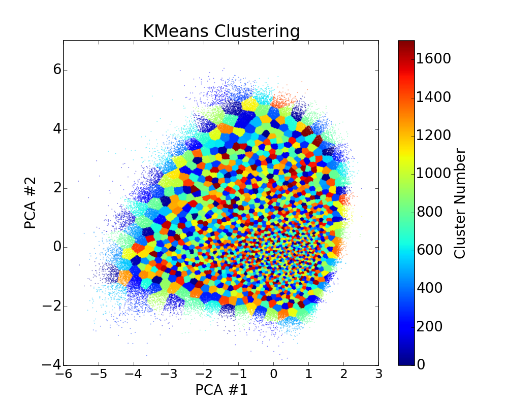
Figure 2 shows the results of k-means clustering when the galaxies are grouped into $(\sqrt{5770490/2})\sim 1700$ clusters. Because there are more galaxies towards the centre of the PCA plane, the Voronoi cells there are smaller compared to the cells around the edges. This achieves the objective of a more even number of galaxies in each cell and hence smaller mean-level differences between the cells.

Figure 2: Clusters identified by k-means algorithm from the PCA projected data. The projected PCA plane has been partitioned to 1700 Voronoi cells. A low value of PCA#1 corresponds to high apparent brightness.

2.5 Statistics of Parameters of Interest: Ellipticities

Now that we have implemented the algorithm described above we can begin to investigate the behaviour of the parameters of interest, in our case the ellipticities of the galaxies used in the weak lensing analysis. In the following the mean and the standard deviation of the ellipticities refer to the weighted versions of these quantities:

$$\left<e_{i}\right> = \frac{\sum w_{i}e_{i}}{\sum w_{i}}$$ (2)

$$\sigma(e_{i}) = \frac{\sum w_{i}(e_{i}-\left<e_{i}\right>)^{2}}{\sum w_{i}}\quad.$$ (3)

The weight $w_{i}$ for a given galaxy $i$ is taken directly from the CFHTLenS catalogue and refers to the inverse variance as calculated by the lensfit algorithm.

2.5.1 Mean

The left panel of Figure 3 shows the mean of the modulus of ellipticity in each of the $1700$ Voronoi cells in Figure 2 identified by the k-means algorithm from the PCA projected data. The colour coding shows low and high mean ellipticity regions with blue and red, respectively. As a sanity check of the data we also calculated the mean of each of the ellipticity component $\left<e_{1}\right>$ and $\left<e_{2}\right>$, which should be consistent with zero in the absence of systematic effects. These were found to be consistent with zero (all Voronoi cells have $-0.015\leq\,\left<e_{i}\right>\,\leq 0.015$).

Figure 3: Left: the mean ellipticity $\left<|e|\right>$ in each of the 1700 Voronoi cells identified by k-means algorithm from the PCA projected data. Right: the standard deviation of modulus of ellipticity $\sigma(|e|)$ of the galaxies in each of the 1700 cells identified by k-means algorithm from the PCA projected data. Three regions of interest, named “A”, “B”, and “C”, have been highlighted. A low value of PCA#1 corresponds to high apparent brightness.

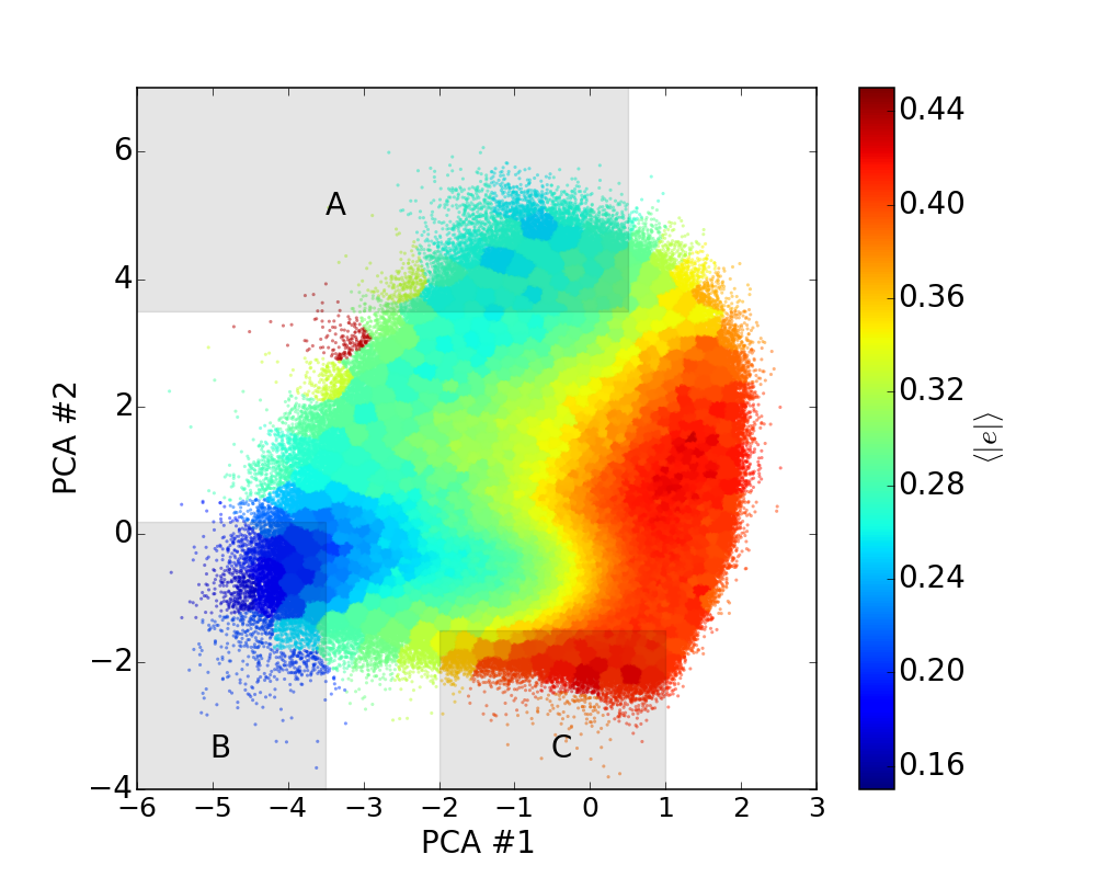
It is remarkable how strongly the average of the modulus of the ellipticity $\left<|e|\right>$ is correlated with the PCA#1 component of the photometry, with a lesser dependence on PCA#2. Given that PCA#1 relates to the visual brightness of a galaxy, this can be explained by three observations. Firstly, at lower redshifts $(z\mathrel{\raise 1.16pt\hbox{$<$}\kern-7.0pt\lower 3.06pt\hbox{{$\scriptstyle\sim$}}}1)$ intrinsically brighter objects are likelier to be more circular from galaxy evolution arguments (e.g. van den Bergh et al., 1996; Conselice et al., 2000): such objects are generally elliptical galaxies instead of spirals, and ellipticals on average have a lower measured $|e|$. Secondly, it is also possible that the galaxies in the low mean ellipticity Voronoi cells are mostly bright face on spiral galaxies, which tend to be less elliptical and visually brighter than more elliptical edge on spirals, which may suffer from substantial dust attenuation in optical wavelengths. In addition, a third effect will arise from what has been termed as ‘noise bias’ (Viola et al., 2014, and references therein) in the weak lensing community. That is, the measured ellipticity of any object is more uncertain (and in general biased towards zero) as the noise level in an image increases. In practice, it is likely that all three competing effects contribute.

2.5.2 Standard Deviation

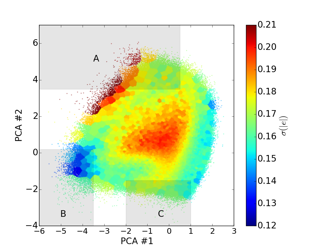
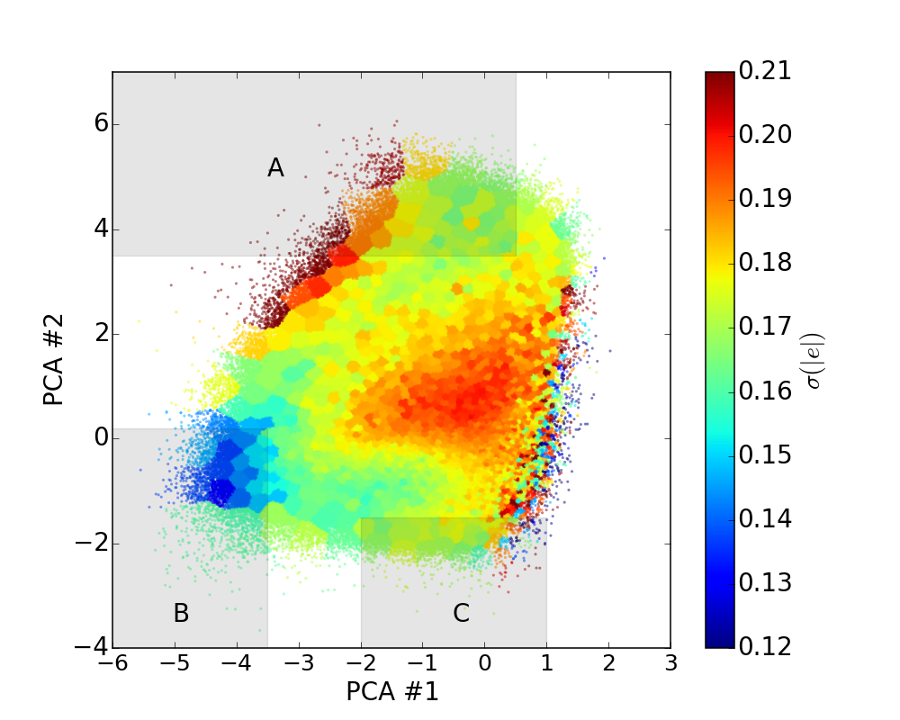
The right panel of Figure 3 shows the standard deviation of the ellipticities of the galaxies in each of the $1700$ Voronoi cells. The figure shows that the region with the highest $\sigma(|e|)$ is at the centre of the projected parameter space and also at the top left corner. Interestingly, the highest mean ellipticity does not correspond to the highest standard deviation regions in the colour-colour principal components plane. The highest ellipticity variance corresponding to PCA#1 values of $\sim 0$ is a significant feature, rather than simply a noise artefact, as we explain below.

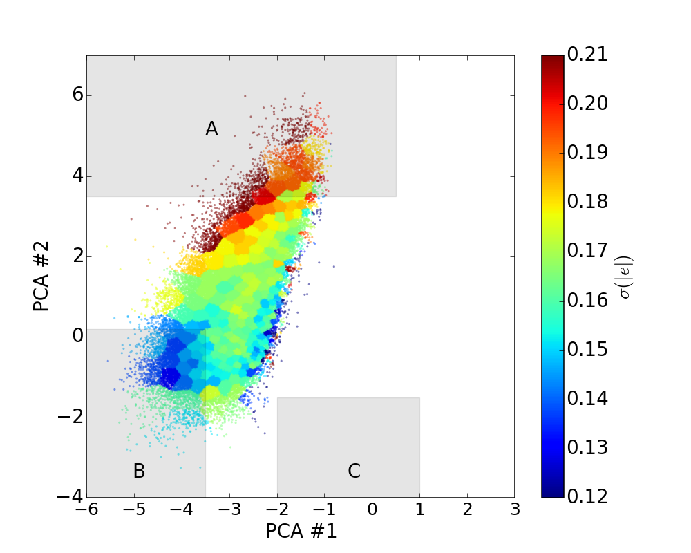
In some cases the high standard deviations could result from larger measurement uncertainties, rather than the intrinsic dispersion. However, in the following we show that the standard deviations over a large part of the PCA plane, especially at high PCA#1 values with the faintest galaxies, are not dominated by measurement errors, but rather the variations in the measured galaxy ellipticities. While the ellipticity measurement for an individual galaxy becomes more uncertain as we move along the PCA#1, simply because the signal-to-noise ratio decreases as the PCA#1 increases, we do not observe the highest dispersions with the highest PCA#1 values. While the noise contribution is a monotonic function of PCA#1, its contribution should not exceed the variance of the cells at a given PCA#1. For all Voronoi cells with the centre of their PCA#1 greater than $1.3$, we find the standard deviation to be $\sim 0.004$ in the ensemble of cells for $\sigma(|e|)$ compared to the typical values of $\sigma(|e|)$ of $\sim 0.14$. Hence, even at the faintest PCA#1 the broadening by measurement noise is not dominant, and it is even less so in all other cells, by thus setting an upper limit for the broadening by measurement noise. To demonstrate this further we have also repeated the analysis at different signal-to-noise ratio slices. The main findings of the paper are largely independent from the selected SNR. Most importantly, the cell statistics remain unchanged when adopting a different SNR cut, only the number of cells populated by galaxies change, as is evident from Figure 4. In the three panels, the SNR selections range from $>10$, $>20$, and $>100$. For the cells that are well populated, the mean ellipticity and the standard deviation remain unchanged.

Figure 4: The standard deviation of modulus of ellipticity $\sigma(|e|)$ of the galaxies in each of the 1700 cells identified by k-means algorithm from the PCA projected data with different signal-to-noise ratio cuts Left: All galaxies with SNR $>10$. Middle: All galaxies with SNR $>20$. Right: All galaxies with SNR $>100$. A low value of PCA#1 corresponds to high apparent brightness and a low value of PCA#2 to a bluer galaxy colour.

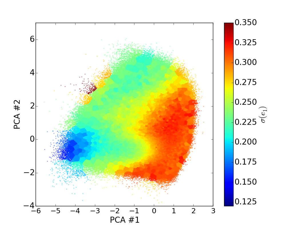
While the right panel of Figure 3 shows the standard deviation of the modulus of the ellipticity, however, for weak lensing analysis the standard deviations of each of the ellipticity components is also of interest. We therefore show the standard deviations for both components separately in Figure 5. It is evident from the Figure that these agree well with each other and also, to some extent, with the mean of the modulus of the ellipticity (the right panel of Figure 3). At high signal to noise we find a similar behaviour, whereas at low signal to noise we find some deviation, where the individual-component variance rises, where the modulus’ variance decreases. This results from two effects that are more pronounced at low signal to noise. Firstly, the standard deviation of the modulus (which is always positive semi-definite), which is approximately a Rayleigh distribution over $0<|\,e\,|<1$, is smaller than the standard deviation that one would compute from a Gaussian over the interval $-1<e_{i}<1$, the relation being a factor of $(4-\pi)/2$. Secondly $e_{1}$ and $e_{2}$ are correlated, thus the standard deviation of the individual components is not expected to fully trace the variance of the modulus. In the remainder of this paper we will investigate the modulus although these considerations should be kept in mind in the interpretation of the results.

Figure 5: Left: the standard deviation of the first ellipticity component $\sigma(e_{1})$ of the galaxies in each of the 1700 cells identified by k-means algorithm from the PCA projected data. Right: the standard deviation of the second ellipticity component $\sigma(e_{2})$ of the galaxies in each of the 1700 cells identified by k-means algorithm from the PCA projected data. A low value of PCA#1 corresponds to high apparent brightness and a low value of PCA#2 to a bluer galaxy colour.

We can also identify broad regions of interest in the PCA plane, these are named “A”, “B”, and “C”, in Figure 3. The “A” region, located at high $(\mathrel{\raise 1.16pt\hbox{$>$}\kern-7.0pt\lower 3.06pt\hbox{{$\scriptstyle\sim$}}}3.5)$ PCA#2 and intermediate $(\mathrel{\raise 1.16pt\hbox{$<$}\kern-7.0pt\lower 3.06pt\hbox{{$\scriptstyle\sim$}}}0.5)$ PCA#1 values, contains Voronoi cells with low or average mean ellipticity, but medium to high standard deviation. Instead, the region “B”, found with the smallest PCA values (PCA#1 $\mathrel{\raise 1.16pt\hbox{$<$}\kern-7.0pt\lower 3.06pt\hbox{{$\scriptstyle\sim$}}}-3.5$ and PCA#2 $\mathrel{\raise 1.16pt\hbox{$<$}\kern-7.0pt\lower 3.06pt\hbox{{$\scriptstyle\sim$}}}0.2$), contains Voronoi cells with the lowest mean ellipticity and standard deviation. This is especially interesting for weak lensing. The third region, named “C”, can be found with the smallest $(\mathrel{\raise 1.16pt\hbox{$<$}\kern-7.0pt\lower 3.06pt\hbox{{$\scriptstyle\sim$}}}-1.5)$ PCA#2 and intermediate $(-2\mathrel{\raise 1.16pt\hbox{$<$}\kern-7.0pt\lower 3.06pt\hbox{{$\scriptstyle\sim$}}}\textrm{PCA\#1}\mathrel{\raise 1.16pt\hbox{$<$}\kern-7.0pt\lower 3.06pt\hbox{{$\scriptstyle\sim$}}}1)$ PCA#1 values, and contains Voronoi cells with the largest mean ellipticity and intermediate standard deviation. It will be interesting to see what types of galaxies reside in these cells. Finally, the rest of the area is covered mostly by cells with either large mean or large standard deviation. We will return to these regions in Section 2.8.

Figure 6: Left: Probability density function for the weighted ellipticity from the galaxies of cell 38 containing mostly very massive elliptical galaxies at intermediate redshifts (region “A”). Middle: Probability density function for the weighted ellipticity from the galaxies of cell 206 containing mostly face-on disk or $S0$-galaxies at relatively low redshift (region “B”). Right: Probability density function for the weighted ellipticity from the galaxies of cell 178 containing mostly inclined disk galaxies at high redshift (region “C”).

2.5.3 Probability Distributions of the Cells

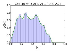
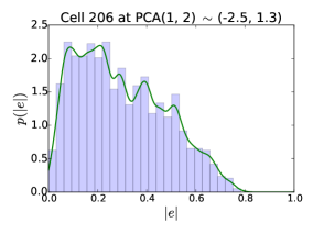
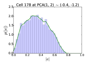
Figure 6 shows the probability density functions (PDFs) for ellipticity derived from all galaxies in a given cell for three different Voronoi cells, corresponding to the three regions described above. These are representative examples. The left panel of Fig. 6 shows the ellipticity PDF of cell number $38$ in Region A, which contains mostly very massive elliptical galaxies at intermediate redshifts. It is clear that the Voronoi cell must also contain some disk or $S0$-galaxies that are inclined because the tail of the PDF extends to higher ellipticities. The middle panel shows the ellipticity PDF of cell number $206$ in region B, which contains mostly face-on disk or $S0$-galaxies at relatively low redshift, peaks at low ellipticity values with a skewness to higher ellipticity values. This will lead to a low mean cluster ellipticity and a relatively small variance. The right panel of Fig. 6 shows the ellipticity PDF of cell number $178$ in Region C, containing mostly inclined disk galaxies at high redshift. The peak of the PDF has now shifted to intermediate ellipticities and the distribution is rather broad leading to a relatively high variance. These panels can be compared to Figure 7 of Joachimi et al. (2013). In general, we find a good agreement. For example, the top panel of Figure 7 of Joachimi et al. (2013) showing the PDF for late-type galaxies is in good qualitative agreement with the right panel of Fig. 6.

2.5.4 Probability Distributions

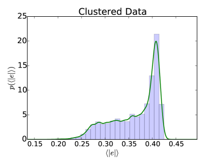
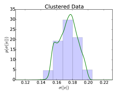
The left panel of Figure 7 shows the ellipticity probability density function derived from all $1700$ Voronoi cells in Figure 2, while the right panel of Figure 7 shows the probability density function of the standard deviation of the ellipticities $p(\sigma(|e|))$. Note that these PDFs (from all cells) are different from those in Fig. 6 (constructed from galaxies within a cell). By selecting galaxies with particular projected PCA values, we can select the appropriate $p(\sigma(|e|))$. In the following Sections we apply this to the case of a weak lensing power spectrum analysis. For example, the $\sigma_{\alpha}(|e|)$ can be tailored to select those particular galaxies (denoted here with $\alpha$) that may be narrower than the all-encompassing $\sigma(|e|)$ for all galaxies. Therefore the shape noise in the power spectrum calculations can be reduced. This will be pursued in Section 3.

Figure 7: Left: probability density function for the weighted mean ellipticity $|e|$ from the clustered data with 1700 individual Voronoi cells. Right: probability density function for the weighted standard deviation of the ellipticity $\sigma(|e|)$ from the clustered data with 1700 individual cells.

2.6 Redshift

The weak lensing power spectrum must be generated at different redshifts to enable weak lensing tomography, as this requires several redshifts to measure the dark energy equation of state (dark energy being an effect that changes the expansion history of the Universe as a function of redshift). It is therefore interesting to look at the redshift distribution of galaxies measured in the CFHTLenS survey in our k-means Voronoi cells. We use the probability density function estimates (full posterior redshift information) from CFHTLenS catalogues, but visualise the point estimate of the PDF. The point estimates presented are the peaks of the PDFs.

Figure 8 shows the mean and the standard deviation of the redshift of the galaxies in each of the $1700$ cells. The figure shows that the highest and the lowest redshift galaxies are separated in different regions in the plane, the lowest average redshift cells favouring the most negative PCA#1 values, while the highest redshift cells can be found with the smallest PCA#2 values. Over a large number of cells the variance between the photometric redshifts of the galaxies in each cell is fairly low, as shown by the right panel of Figure 8.

Figure 8: Left: the mean redshift $\left<z\right>$ in each of the 1700 Voronoi cells identified by k-means algorithm from the PCA projected data. Right: the standard deviation of the redshift $\sigma(z)$ of the galaxies in each of the 1700 Voronoi cells identified by k-means algorithm from the PCA projected data. A low value of PCA#1 corresponds to high apparent brightness.

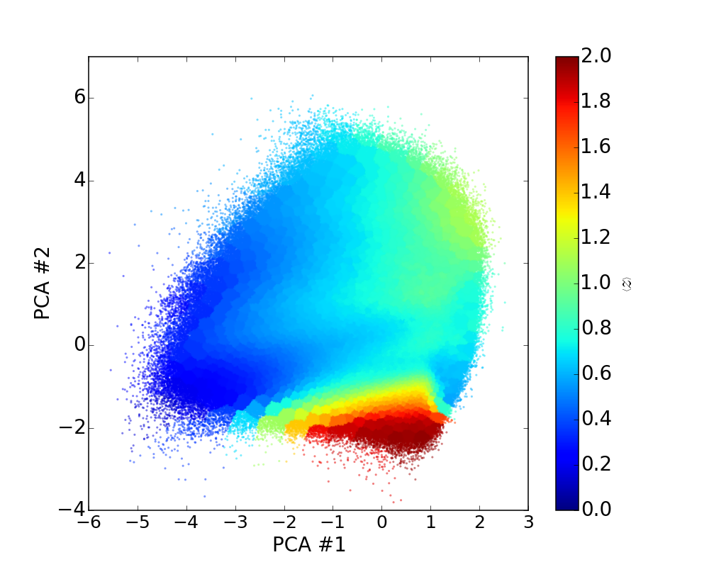
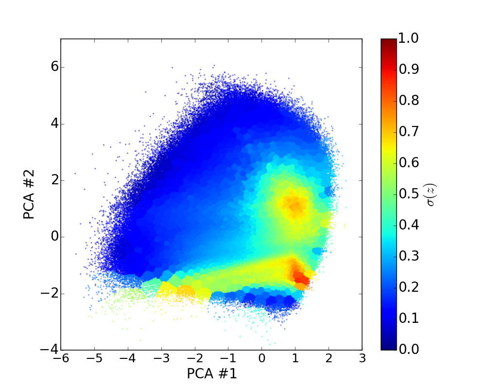
2.7 Galaxy Properties

In the previous sections we have looked at the average properties of the galaxies in the Voronoi cells, which are relevant for weak gravitational lensing. However, because of the clear trends in the average ellipticities as shown by the left panel of Figure 3 it is interesting to look also at the astrophysical properties of these galaxies. There are many parameters that describe galaxy morphology and astrophysical properties, here we chose one that was derived from the CFHTLenS ellipticity measurements (using lensfit; the bulge-to-disc ratio) and one that was derived from photometric measurements (the stellar mass) for comparison. However this approach could be generalised to any property listed in a catalogue.

2.7.1 Bulge-to-Disc Ratios

A fundamental galaxy property is the bulge-to-disc ratio, which can be used as a proxy for the morphological type of a galaxy (e.g. Simien & de Vaucouleurs, 1986). Figure 9 shows the mean and the standard deviation of the bulge fractions of the galaxies measured in the CFHTLenS (column BULGE_FRACTION in the CFHTLenS catalogue) in each of the $1700$ k-means clusters. A clear trend can be observed; the smaller the PCA#1 and higher the PCA#2 value, the higher the average bulge fraction. Thus, galaxies in these Voronoi cells are more likely to be bulge dominated elliptical galaxies. If this is true, there should also be a similar trend in the average stellar masses.

Figure 9: Left: the mean bulge fraction in each of the 1700 Voronoi cells identified by k-means algorithm from the PCA projected data. Right: the standard deviation of the bulge fraction of the galaxies in each of the 1700 Voronoi cells identified by k-means algorithm from the PCA projected data. A low value of PCA#1 corresponds to high apparent brightness.

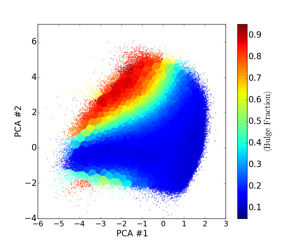
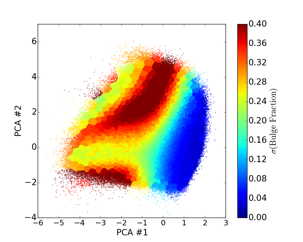
2.7.2 Stellar Masses

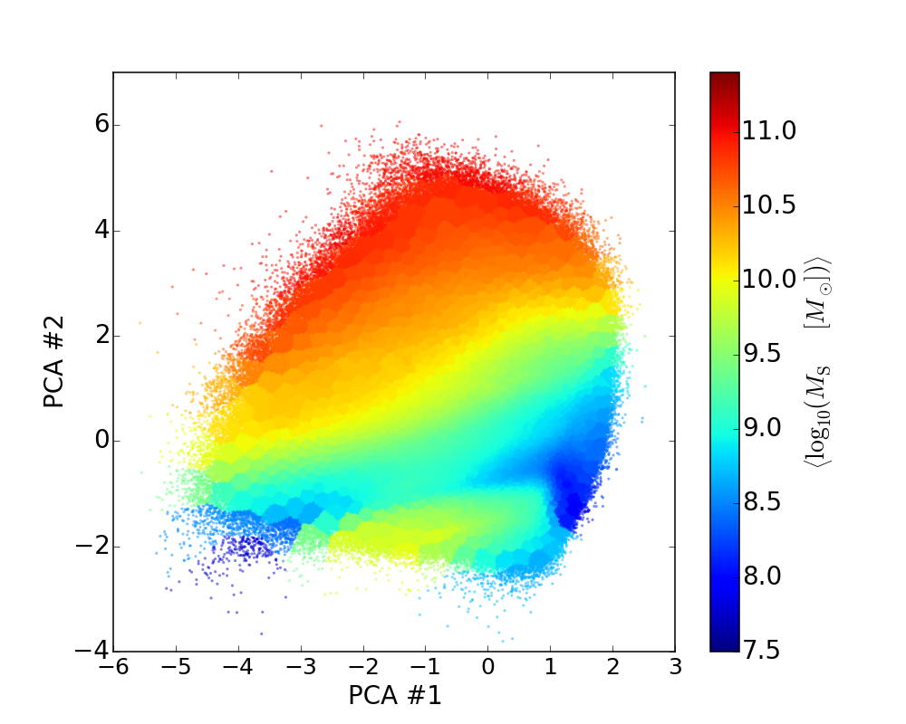
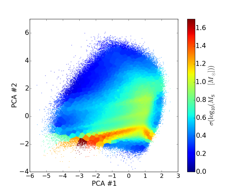
For the stellar masses we use the LP_log10_SM_MED column of the CFHTLenS catalogue, which contains the median estimate for the stellar mass. The missing values, indicated by $-99$, were omitted from the calculations. Figure 10 shows the mean and the standard deviation of the stellar masses of the galaxies in each of the $1700$ k-means Voronoi cells. A clear trend along the PCA#2 can be observed: higher values of the PCA component correspond to average higher stellar masses, which is as expected because stellar mass is related to galaxy colour. This agrees with the interpretation of the bulge-to-disc ratio results for the location of elliptical galaxies in the PCA plane.

Figure 10: Left: the mean stellar mass $\left<\log_{10}(M_{S}\,[M_{\odot}])\right>$ in each of the 1700 Voronoi cells identified by k-means algorithm from the PCA projected data. Right: the standard deviation of the stellar mass $\sigma(\log_{10}(M_{S}\,[M_{\odot}]))$ of the galaxies in each of the 1700 Voronoi cells identified by k-means algorithm from the PCA projected data. A low value of PCA#1 corresponds to high apparent brightness.

2.8 Regions of Interest

The three regions, “A”, “B”, and “C”, identified earlier can now be linked to different galaxy types. For example, the Voronoi cells in region “A”, that is the highest $(\mathrel{\raise 1.16pt\hbox{$>$}\kern-7.0pt\lower 3.06pt\hbox{{$\scriptstyle\sim$}}}3.5)$ PCA#2 and intermediate $(\mathrel{\raise 1.16pt\hbox{$<$}\kern-7.0pt\lower 3.06pt\hbox{{$\scriptstyle\sim$}}}0.5)$ PCA#1 values, contain very massive elliptical galaxies, which reside on average at an intermediate redshifts $(\left<z\right>\sim 0.7)$. Region “B”, with the smallest PCA values (PCA#1 $\mathrel{\raise 1.16pt\hbox{$<$}\kern-7.0pt\lower 3.06pt\hbox{{$\scriptstyle\sim$}}}-3.5$ and PCA#2 $\mathrel{\raise 1.16pt\hbox{$<$}\kern-7.0pt\lower 3.06pt\hbox{{$\scriptstyle\sim$}}}0.2$), contains cells with mostly relatively low mass (see Fig. 10) face-on disk or $S0$-galaxies (Fig. 9) who reside relative nearby (low redshift, see Fig. 8). The highest redshift $(\left<z\right>\sim 2)$ disk galaxies, which are also often inclined, can be found in region “C” with the smallest $(\mathrel{\raise 1.16pt\hbox{$<$}\kern-7.0pt\lower 3.06pt\hbox{{$\scriptstyle\sim$}}}-1.5)$ PCA#2 and intermediate $(-2\mathrel{\raise 1.16pt\hbox{$<$}\kern-7.0pt\lower 3.06pt\hbox{{$\scriptstyle\sim$}}}\textrm{PCA\#1}\mathrel{\raise 1.16pt\hbox{$<$}\kern-7.0pt\lower 3.06pt\hbox{{$\scriptstyle\sim$}}}1)$ PCA#1 values.

3 Application: Improved Parameter Inference

3.1 Context

Once the distribution functions of the statistical properties of parameters of interest are available as a function of meta-parameters, these can then be used to improve the inferences made on model parameters that one may wish to fit to the data. This approach is tied very closely to the approach of Bayesian Hierarchical modelling (e.g. Schneider et al., 2014), and indeed the distribution functions uncovered using our approach can be used as initial input into a Bayesian network where prior probability distributions of meta-parameters and parameters of interest are required in order to efficiently sample the joint likelihood space investigated. When including a full model of the data in such an approach, the aggregated gains commonly lead to improved parameter precision and accuracy (as has been seen in a supernovae application in cosmology, see e.g. Mandel et al. (2009); Mandel et al. (2011)).

In this paper we apply the distribution of the standard deviation of ellipticity in a more simple, but also pedagogical, manner where we extend the weak lensing power spectrum formalism to include such a distribution and assess the change in expected cosmological parameter performance derived from such an analysis.

3.2 Generalised Cosmic Shear Power Spectra

Previous cosmic shear analyses use a single population of galaxies (or split into two samples e.g. Heymans et al. (2013)), after selections are made at the shape measurement stage, and a single ellipticity variance calculated and applied to calculate a single cosmic shear power spectrum. This would correspond to a delta-function distribution in the right panel of Figure 7. In our case the data can be subdivided into several sub-populations, each with a different number density $n_{\alpha}(z)$ and ellipticity variance $\sigma^{2}_{\alpha}(|e|)$ (henceforth shortened to $\sigma^{2}_{e,\alpha}$), these can be combined in a more optimal way.

The observed tomographic cosmic shear power spectrum (see Hu, 1999) can be written as a sum of a signal and noise term

$$C_{ij,\ell}=C^{S}_{ij,\ell}+N_{ij,\ell}\quad,$$ (4)

where $ij$ refer to redshift bin pairs (such that $i=j$ refers to intra-bin power or ‘auto-correlation’, and $i\not=j$ refers to inter-bin power or ‘cross-correlation’), and $\ell$ refers to an angular wavenumber. We refer the reader to Kitching et al. (2011) where this is derived from a spherical harmonic-spherical Bessel representation of the full three-dimensional shear field.

The signal part of the power spectrum $C^{S}$ is a function of angular diameter distances of the source redshift, and a function of the matter power spectrum as a function of redshift (or comoving distance):

$$C_{ij,\ell}^{S}=A\int_{0}^{r(z_{H})}{\rm d}r^{\prime}\frac{W_{i}(r^{\prime})W_{j}(r^{\prime})}{a(r^{\prime})^{2}}P(\ell/r^{\prime};r[z])\quad.$$ (5)

The constant $A=(3\Omega_{\rm M}H_{0}^{2}/2c^{2})^{2}$, where $\Omega_{\rm M}$ is the dimensionless matter density, $H_{0}$ is the current value of the Hubble parameter, $z_{H}$ is the redshift of the cosmic horizon, $c$ is the speed of light in a vacuum, $a(r)$ is the dimensionless scale factor, $P(\ell/r;r(z))$ is the power spectrum of matter perturbations, and $r(z)$ is a comoving distance. The weight function is

$$W_{i}(r)=\int_{r}^{r(z_{H})}{\rm d}{r^{\prime}}p(r^{\prime}|r[z_{i}])\frac{f_{K}(r^{\prime}-r)}{f_{K}(r^{\prime})}\quad,$$ (6)

where $f_{K}(r)=\sinh(r)$, $r$, $\sin(r)$ for curvatures of $K=-1$, $0$, $1$, and $p(r^{\prime}\,|\,r)$ is the probability that a galaxy with comoving distance $r$ is observed at distance $r^{\prime}$. This representation of the shear power spectrum assumes the Limber approximation, a spherical Bessel transform to comoving distance, and a binning in redshift; for a derivation of this from the full 3D cosmic shear power spectrum see Kitching et al. (2011).

The noise part of the power spectrum is

$$N_{ij,\ell}=\frac{\sigma_{e}^{2}\delta^{K}_{ij}}{\bar{N}_{ii}}\quad,$$ (7)

where $\sigma^{2}_{e}$ is the ellipticity variance, $\delta^{K}$ is a Kroneger delta-function, and $\bar{N}_{ii}$ is the mean number of galaxies in redshift bin $i$. To minimise the noise contribution, one should aim to maximise the mean number of galaxies, while minimising the ellipticity variance.

For each $N_{\rm bin}$ galaxy populations, each with a different number density and ellipticity variance, derived using the process described in the previous Section, the power spectra can be combined using an inverse-variance weighted sum

$$\overline{C}_{ij,\ell}=\frac{\sum_{\alpha}^{N_{\rm bin}}(1/\sigma^{2}_{e,\alpha})C^{\alpha}_{ij,\ell}}{\sum_{\alpha}^{N_{\rm bin}}(1/\sigma^{2}_{e,\alpha})}\quad,$$ (8)

where $C^{\alpha}_{ij,\ell}$ is the power spectrum computed for the population $\alpha$, that has a number density $n_{\alpha}(z)$ and an ellipticity variance $\sigma^{2}_{e,\alpha}$. We assume here that each population is subdivided into the same redshift bin set, although this can in principle also change between the populations.

3.3 Applying the Inverse Weighting

Here we present a prediction for how such weighting will impact cosmological parameter estimation using tomographic cosmic shear. To compute expected cosmological parameter errors we use the Fisher matrix formalism present in Hu (1999) for cosmic shear tomography. This results in a matrix $F_{\alpha\beta}$ (the Greek letters denote cosmological parameters) where the $[(F^{-1})_{\alpha\alpha}]^{1/2}$ is a vector of expected, marginalised, cosmological parameter uncertainties. We use a Cold Dark Matter (CDM) cosmology with a varying dark energy equation of state, where the free parameters that we use are $\Omega_{\rm M}$, $\Omega_{\rm B}$, $\sigma_{8}$, $w_{0}$, $w_{a}$, $h$, $n_{s}$ (respectively, the dimensionless matter density; dimensionless baryon density; the amplitude of matter fluctuations on $8$Mpc scales – a normalisation of the power spectrum of matter perturbations; the dark energy equation of state parametrised by $w(z)=w_{0}+w_{a}z/(1+z)$; the Hubble parameter $h=H_{0}/100$kms^-1Mpc^-1; and the scalar spectral index of initial matter perturbations). For each parameter we use the Planck maximum likelihood values (Planck Collaboration et al., 2014a, b) about which to take derivative of the power spectra for the Fisher matrix. All parameter errors and biases we quote are marginalised over all other parameters in this set. We use the camb sources code (see http://camb.info/sources/ and Seljak & Zaldarriaga, 1996; Lewis & Bridle, 2002; Challinor & Lewis, 2011) to compute the cosmic shear tomographic power spectra. We use a maximum radial wavenumber of $k_{\rm max}=10h$Mpc^-1 and a corresponding redshift-dependent maximum $\ell$-mode of $\ell=k_{\rm max}r[z]$.

The cosmic shear survey we assume is a Euclid-like experiment that has an area of $15000$ square degrees, a median redshift of $z_{m}=0.9$, a number density of $30$ galaxies per square arcminute with a number density distribution $n(z)$ given in Taylor et al. (2007), and a photometric redshift distribution that is assumed to be Gaussian with a standard deviation of $\sigma(z)=0.05(1+z)$. These characteristic are described in Laureijs et al. (2011).

To investigate the expected effect we first look at some simple model examples to illustrate the essential aspects of the information change that occurs when including a more general distribution of the $p(\sigma)$. We use the probability distribution of the variance shown in the right panel of Figure 7, and assume that the number density distribution as a function of redshift is the same for each population. We compare with the standard case, where the mean of the variance is taken from the distribution in the right panel of Figure 7 and a single population is assumed. We find that the inclusion of the inverse-variance weighting, in this case, improves the predicted dark energy Figure-of-Merit ($1/(\sigma(w_{0})\sigma(w_{a})-[\sigma^{2}(w_{0},w_{a})])$) (Albrecht et al., 2006) by a modest two per cent. However, this improvement demonstrates the principle of the improvement that may be gained, and this will be more significant when several such meta-parameters of the data are combined.

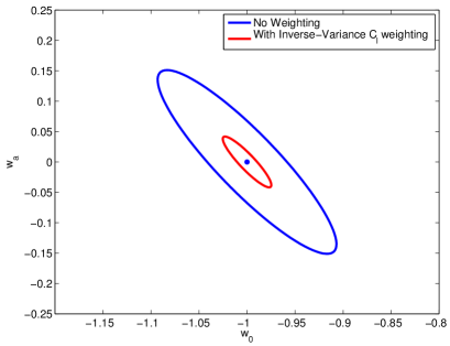
To demonstrate the principle further, we show in Figure 11 the $(w_{0},w_{a})$ predicted projected $1\sigma$ uncertainty contours for the case in which no $\sigma_{e}$ weighting is used and the case in which half of the galaxies have a $\sigma_{e}$ which is half the nominal case i.e. the distribution is a top hat function from $0.15$ to $0.30$. It is clear from this Figure that if additional meta-parameters can be found, such that Voronoi cells with small ellipticity variance can be identified, significant gains can be made, and this would in fact become the dominant consideration in supplementing weak lensing surveys for dark energy science. Using supplementary data such as that discussed in Huff et al. (2013) there remains the possibility of finding such a low-$\sigma_{e}$ measure or population of galaxies.

Figure 11: The predicted marginalised 2-parameter $1\sigma$ uncertainty ellipsoids in the $(w_{0},w_{a})$ plane with and without the inverse-variance weighting, for a Euclid-like experiment in case half of the galaxies have half the ellipticity standard deviation.

4 Conclusion

In this paper we present a method that can be used to find how the probability distributions of parameters of interest depend on other, meta-parameters in the data. This uses a dimensionality reduction and noise whitening, followed by a clustering analysis. We use this to investigate how the probability distributions of galaxy ellipticity depend on photometry of galaxies. In particular we construct a probability distribution for the intrinsic standard deviation of the galaxy ellipticities $p(\sigma(|e|))$.

We apply this to the investigation of galaxy properties and find that such an approach is particularly good at isolating galaxy type: where regions in the clustering analysis correspond to early and late type galaxies. Finally, we apply this to the case of improving cosmological parameter inference using weak lensing and find a few percent improvement in dark energy measurements even in this simple application.

The method we use here has several applications as a tool for cosmology, and has synergies with a full Bayesian hierarchical modelling approach.

Acknowledgements: The authors thank the anonymous reviewer whose comments helped to improve the manuscript. TDK is supported by a Royal Society University Research Fellowship. We thank the CFHTLenS team for making their catalogues public. We also thank Jason McEwen and Ignacio Ferreras for useful discussions.

References

- Albrecht et al. (2006) Albrecht A., et al., 2006, ArXiv Astrophysics e-prints, \hrefhttp://adsabs.harvard.edu/abs/2006astro.ph..9591A
- Amendola et al. (2013) Amendola L., et al., 2013, \hrefhttp://dx.doi.org/10.12942/lrr-2013-6 Living Reviews in Relativity, \hrefhttp://adsabs.harvard.edu/abs/2013LRR….16….6A 16, 6
- Bartelmann & Schneider (2001) Bartelmann M., Schneider P., 2001, \hrefhttp://dx.doi.org/10.1016/S0370-1573(00)00082-X Phys. Rep., \hrefhttp://adsabs.harvard.edu/abs/2001PhR…340..291B 340, 291
- Bengio et al. (2012) Bengio Y., Courville A., Vincent P., 2012, preprint, \hrefhttp://adsabs.harvard.edu/abs/2012arXiv1206.5538B (\hrefhttp://arxiv.org/abs/1206.5538 arXiv:1206.5538)
- Benítez (2000) Benítez N., 2000, \hrefhttp://dx.doi.org/10.1086/308947 Astro. Phys. Journal, \hrefhttp://adsabs.harvard.edu/abs/2000ApJ…536..571B 536, 571
- Benjamin et al. (2007) Benjamin J., et al., 2007, \hrefhttp://dx.doi.org/10.1111/j.1365-2966.2007.12202.x MNRAS, \hrefhttp://adsabs.harvard.edu/abs/2007MNRAS.381..702B 381, 702
- Bennett et al. (2013) Bennett C. L., et al., 2013, \hrefhttp://dx.doi.org/10.1088/0067-0049/208/2/20 ApJS, \hrefhttp://adsabs.harvard.edu/abs/2013ApJS..208…20B 208, 20
- Cao et al. (1994) Cao R., Cuevas A., Manteiga W. G., 1994, \hrefhttp://dx.doi.org/10.1016/0167-9473(92)00066-Z Computational Statistics & Data Analysis, 17, 153
- Challinor & Lewis (2011) Challinor A., Lewis A., 2011, \hrefhttp://dx.doi.org/10.1103/PhysRevD.84.043516 Phys.Rev., D84, 043516
- Clifton et al. (2012) Clifton T., Ferreira P. G., Padilla A., Skordis C., 2012, \hrefhttp://dx.doi.org/10.1016/j.physrep.2012.01.001 Phys. Rep., \hrefhttp://adsabs.harvard.edu/abs/2012PhR…513….1C 513, 1
- Coe et al. (2006) Coe D., Benítez N., Sánchez S. F., Jee M., Bouwens R., Ford H., 2006, \hrefhttp://dx.doi.org/10.1086/505530 Astronomical Journal, \hrefhttp://adsabs.harvard.edu/abs/2006AJ….132..926C 132, 926
- Conselice et al. (2000) Conselice C. J., Bershady M. A., Jangren A., 2000, \hrefhttp://dx.doi.org/10.1086/308300 Astro. Phys. Journal, \hrefhttp://cdsads.u-strasbg.fr/abs/2000ApJ…529..886C 529, 886
- Ding & He (2004) Ding He X., 2004, Proc. of Int’l Conf. Machine Learning
- Duncan et al. (2014) Duncan C. A. J., Joachimi B., Heavens A. F., Heymans C., Hildebrandt H., 2014, \hrefhttp://dx.doi.org/10.1093/mnras/stt2060 MNRAS, \hrefhttp://adsabs.harvard.edu/abs/2014MNRAS.437.2471D 437, 2471
- Erben et al. (2013) Erben T., et al., 2013, \hrefhttp://dx.doi.org/10.1093/mnras/stt928 MNRAS, \hrefhttp://adsabs.harvard.edu/abs/2013MNRAS.433.2545E 433, 2545
- Fu et al. (2008) Fu L., et al., 2008, \hrefhttp://dx.doi.org/10.1051/0004-6361:20078522 AAP, \hrefhttp://adsabs.harvard.edu/abs/2008A
- Halko et al. (2009) Halko N., Martinsson P.-G., Tropp J. A., 2009, preprint, \hrefhttp://adsabs.harvard.edu/abs/2009arXiv0909.4061H (\hrefhttp://arxiv.org/abs/0909.4061 arXiv:0909.4061)
- Hastie et al. (2001) Hastie T., Tibshirani R., Friedman J., 2001, The Elements of Statistical Learning. Springer Series in Statistics, Springer New York Inc., New York, NY, USA
- Heymans et al. (2012) Heymans C., et al., 2012, \hrefhttp://dx.doi.org/10.1111/j.1365-2966.2012.21952.x MNRAS, \hrefhttp://adsabs.harvard.edu/abs/2012MNRAS.427..146H 427, 146
- Heymans et al. (2013) Heymans C., et al., 2013, \hrefhttp://dx.doi.org/10.1093/mnras/stt601 MNRAS, \hrefhttp://adsabs.harvard.edu/abs/2013MNRAS.432.2433H 432, 2433
- Hildebrandt et al. (2012) Hildebrandt H., et al., 2012, \hrefhttp://dx.doi.org/10.1111/j.1365-2966.2012.20468.x MNRAS, \hrefhttp://adsabs.harvard.edu/abs/2012MNRAS.421.2355H 421, 2355
- Hoekstra & Jain (2008) Hoekstra H., Jain B., 2008, \hrefhttp://dx.doi.org/10.1146/annurev.nucl.58.110707.171151 Annual Review of Nuclear and Particle Science, \hrefhttp://adsabs.harvard.edu/abs/2008ARNPS..58…99H 58, 99
- Hu (1999) Hu W., 1999, \hrefhttp://dx.doi.org/10.1086/312210 Astro. Phys. Journal Letters, \hrefhttp://adsabs.harvard.edu/abs/1999ApJ…522L..21H 522, L21
- Huff et al. (2013) Huff E. M., Krause E., Eifler T., George M. R., Schlegel D., 2013, preprint, \hrefhttp://adsabs.harvard.edu/abs/2013arXiv1311.1489H (\hrefhttp://arxiv.org/abs/1311.1489 arXiv:1311.1489)
- Jaffe et al. (2005) Jaffe T. R., Banday A. J., Eriksen H. K., Górski K. M., Hansen F. K., 2005, \hrefhttp://dx.doi.org/10.1086/444454 Astro. Phys. Journal Letters, \hrefhttp://adsabs.harvard.edu/abs/2005ApJ…629L…1J 629, L1
- Joachimi et al. (2013) Joachimi B., Semboloni E., Bett P. E., Hartlap J., Hilbert S., Hoekstra H., Schneider P., Schrabback T., 2013, \hrefhttp://dx.doi.org/10.1093/mnras/stt172 Monthly Notices of the Royal Astronomical Society, 431, 477
- Kaiser (1992) Kaiser N., 1992, \hrefhttp://dx.doi.org/10.1086/171151 Astro. Phys. Journal, \hrefhttp://adsabs.harvard.edu/abs/1992ApJ…388..272K 388, 272
- Kilbinger et al. (2013) Kilbinger M., et al., 2013, \hrefhttp://dx.doi.org/10.1093/mnras/stt041 MNRAS, \hrefhttp://adsabs.harvard.edu/abs/2013MNRAS.430.2200K 430, 2200
- Kitching et al. (2007) Kitching T. D., Heavens A. F., Taylor A. N., Brown M. L., Meisenheimer K., Wolf C., Gray M. E., Bacon D. J., 2007, \hrefhttp://dx.doi.org/10.1111/j.1365-2966.2007.11473.x MNRAS, \hrefhttp://adsabs.harvard.edu/abs/2007MNRAS.376..771K 376, 771
- Kitching et al. (2011) Kitching T. D., Heavens A. F., Miller L., 2011, \hrefhttp://dx.doi.org/10.1111/j.1365-2966.2011.18369.x MNRAS, \hrefhttp://adsabs.harvard.edu/abs/2011MNRAS.413.2923K 413, 2923
- Kitching et al. (2014) Kitching T. D., et al., 2014, \hrefhttp://dx.doi.org/10.1093/mnras/stu934 MNRAS, \hrefhttp://adsabs.harvard.edu/abs/2014MNRAS.442.1326K 442, 1326
- Kohonen (1982) Kohonen T., 1982, \hrefhttp://dx.doi.org/10.1007/BF00337288 Biological Cybernetics, 43, 59
- Komatsu et al. (2011) Komatsu E., et al., 2011, \hrefhttp://dx.doi.org/10.1088/0067-0049/192/2/18 ApJS, \hrefhttp://adsabs.harvard.edu/abs/2011ApJS..192…18K 192, 18
- Laureijs et al. (2011) Laureijs R., et al., 2011, preprint, \hrefhttp://adsabs.harvard.edu/abs/2011arXiv1110.3193L (\hrefhttp://arxiv.org/abs/1110.3193 arXiv:1110.3193)
- Laureijs et al. (2012) Laureijs R., et al., 2012, in Society of Photo-Optical Instrumentation Engineers (SPIE) Conference Series. , \hrefhttp://dx.doi.org/10.1117/12.926496 doi:10.1117/12.926496
- Lewis & Bridle (2002) Lewis A., Bridle S., 2002, Phys. Rev., D66, 103511
- MacQueen (1967) MacQueen J., 1967, Some methods for classification and analysis of multivariate observations., Proc. 5th Berkeley Symp. Math. Stat. Probab., Univ. Calif. 1965/66, 1, 281-297 (1967).
- Mandel et al. (2009) Mandel K. S., Wood-Vasey W. M., Friedman A. S., Kirshner R. P., 2009, \hrefhttp://dx.doi.org/10.1088/0004-637X/704/1/629 Astro. Phys. Journal, \hrefhttp://adsabs.harvard.edu/abs/2009ApJ…704..629M 704, 629
- Mandel et al. (2011) Mandel K. S., Narayan G., Kirshner R. P., 2011, \hrefhttp://dx.doi.org/10.1088/0004-637X/731/2/120 Astro. Phys. Journal, \hrefhttp://adsabs.harvard.edu/abs/2011ApJ…731..120M 731, 120
- Massey et al. (2010) Massey R., Kitching T., Richard J., 2010, \hrefhttp://dx.doi.org/10.1088/0034-4885/73/8/086901 Reports on Progress in Physics, \hrefhttp://adsabs.harvard.edu/abs/2010RPPh…73h6901M 73, 086901
- McEwen et al. (2013) McEwen J. D., Josset T., Feeney S. M., Peiris H. V., Lasenby A. N., 2013, \hrefhttp://dx.doi.org/10.1093/mnras/stt1855 MNRAS, \hrefhttp://adsabs.harvard.edu/abs/2013MNRAS.436.3680M 436, 3680
- Miller et al. (2007) Miller L., Kitching T. D., Heymans C., Heavens A. F., Van Waerbeke L., 2007, \hrefhttp://dx.doi.org/10.1111/j.1365-2966.2007.12363.x Monthly Notices of the Royal Astronomical Society, 382, 315
- Miller et al. (2013) Miller L., et al., 2013, \hrefhttp://dx.doi.org/10.1093/mnras/sts454 Monthly Notices of the Royal Astronomical Society, 429, 2858
- Munshi et al. (2008) Munshi D., Valageas P., van Waerbeke L., Heavens A., 2008, \hrefhttp://dx.doi.org/10.1016/j.physrep.2008.02.003 Phys. Rep., \hrefhttp://adsabs.harvard.edu/abs/2008PhR…462…67M 462, 67
- Parzen (1962) Parzen E., 1962, \hrefhttp://dx.doi.org/10.1214/aoms/1177704472 Ann. Math. Statist., 33, 1065
- Peacock et al. (2006) Peacock J. A., Schneider P., Efstathiou G., Ellis J. R., Leibundgut B., Lilly S. J., Mellier Y., 2006, Technical report, ESA-ESO Working Group on ”Fundamental Cosmology”. (\hrefhttp://arxiv.org/abs/astro-ph/0610906 arXiv:astro-ph/0610906)
- Pearson (1901) Pearson K., 1901, \hrefhttp://dx.doi.org/10.1080/14786440109462720 Philosophical Magazine Series 6, 2, 559
- Pedregosa et al. (2011) Pedregosa F., et al., 2011, Journal of Machine Learning Research, 12, 2825
- Perlmutter et al. (1999) Perlmutter S., et al., 1999, \hrefhttp://dx.doi.org/10.1086/307221 Astro. Phys. Journal, \hrefhttp://adsabs.harvard.edu/abs/1999ApJ…517..565P 517, 565
- Planck Collaboration (2015) Planck Collaboration 2015, preprint, \hrefhttp://adsabs.harvard.edu/abs/2015arXiv150201589P (\hrefhttp://arxiv.org/abs/1502.01589 arXiv:1502.01589)
- Planck Collaboration et al. (2014a) Planck Collaboration et al., 2014a, \hrefhttp://dx.doi.org/10.1051/0004-6361/201321573 AAP, \hrefhttp://adsabs.harvard.edu/abs/2014A
- Planck Collaboration et al. (2014b) Planck Collaboration et al., 2014b, \hrefhttp://dx.doi.org/10.1051/0004-6361/201321591 AAP, \hrefhttp://adsabs.harvard.edu/abs/2014A
- Planck Collaboration et al. (2014c) Planck Collaboration et al., 2014c, \hrefhttp://dx.doi.org/10.1051/0004-6361/201321546 AAP, \hrefhttp://adsabs.harvard.edu/abs/2014A
- Planck Collaboration et al. (2015) Planck Collaboration et al., 2015, preprint, \hrefhttp://adsabs.harvard.edu/abs/2015arXiv150201593P (\hrefhttp://arxiv.org/abs/1502.01593 arXiv:1502.01593)
- Riess et al. (1998) Riess A. G., et al., 1998, \hrefhttp://dx.doi.org/10.1086/300499 Astronomical Journal, \hrefhttp://adsabs.harvard.edu/abs/1998AJ….116.1009R 116, 1009
- Rosenblatt (1956) Rosenblatt M., 1956, \hrefhttp://dx.doi.org/10.1214/aoms/1177728190 Ann. Math. Statist., 27, 832
- Rudemo (1982) Rudemo M., 1982, Scandinavian Journal of Statistics, 9, pp. 65
- Schneider et al. (2014) Schneider M. D., Hogg D. W., Marshall P. J., Dawson W. A., Meyers J., Bard D. J., Lang D., 2014, preprint, \hrefhttp://adsabs.harvard.edu/abs/2014arXiv1411.2608S (\hrefhttp://arxiv.org/abs/1411.2608 arXiv:1411.2608)
- Schrabback et al. (2010) Schrabback T., et al., 2010, \hrefhttp://dx.doi.org/10.1051/0004-6361/200913577 AAP, \hrefhttp://adsabs.harvard.edu/abs/2010A
- Seljak & Zaldarriaga (1996) Seljak U., Zaldarriaga M., 1996, Astrophys. J., 469, 437
- Semboloni et al. (2006) Semboloni E., et al., 2006, \hrefhttp://dx.doi.org/10.1051/0004-6361:20054479 AAP, \hrefhttp://adsabs.harvard.edu/abs/2006A
- Simien & de Vaucouleurs (1986) Simien F., de Vaucouleurs G., 1986, \hrefhttp://dx.doi.org/10.1086/164015 Astro. Phys. Journal, \hrefhttp://adsabs.harvard.edu/abs/1986ApJ…302..564S 302, 564
- Steinhaus (1957) Steinhaus H., 1957, Bull. Acad. Pol. Sci., Cl. III, 4, 801
- Taylor et al. (2007) Taylor A. N., Kitching T. D., Bacon D. J., Heavens A. F., 2007, \hrefhttp://dx.doi.org/10.1111/j.1365-2966.2006.11257.x MNRAS, \hrefhttp://adsabs.harvard.edu/abs/2007MNRAS.374.1377T 374, 1377
- Viola et al. (2014) Viola M., Kitching T. D., Joachimi B., 2014, \hrefhttp://dx.doi.org/10.1093/mnras/stu071 MNRAS, \hrefhttp://adsabs.harvard.edu/abs/2014MNRAS.439.1909V 439, 1909
- Weinberg et al. (2013) Weinberg D. H., Mortonson M. J., Eisenstein D. J., Hirata C., Riess A. G., Rozo E., 2013, \hrefhttp://dx.doi.org/10.1016/j.physrep.2013.05.001 Phys. Rep., \hrefhttp://adsabs.harvard.edu/abs/2013PhR…530…87W 530, 87
- Zha et al. (2001) Zha H., Ding C., Gu M., He X., Simon H., 2001, Neural Information Processing Systems, 14
- van den Bergh et al. (1996) van den Bergh S., Abraham R. G., Ellis R. S., Tanvir N. R., Santiago B. X., Glazebrook K. G., 1996, \hrefhttp://dx.doi.org/10.1086/118020 Astronomical Journal, \hrefhttp://cdsads.u-strasbg.fr/abs/1996AJ….112..359V 112, 359