Group Membership Prediction

Abstract

The group membership prediction (GMP) problem involves predicting whether or not a collection of instances share a certain semantic property. For instance, in kinship verification given a collection of images, the goal is to predict whether or not they share a familial relationship. In this context we propose a novel probability model and introduce latent view-specific and view-shared random variables to jointly account for the view-specific appearance and cross-view similarities among data instances. Our model posits that data from each view is independent conditioned on the shared variables. This postulate leads to a parametric probability model that decomposes group membership likelihood into a tensor product of data-independent parameters and data-dependent factors. We propose learning the data-independent parameters in a discriminative way with bilinear classifiers, and test our prediction algorithm on challenging visual recognition tasks such as multi-camera person re-identification and kinship verification. On most benchmark datasets, our method can significantly outperform the current state-of-the-art.

1 Introduction

Visual similarity plays an important role in visual recognition in object detection and scene understanding [11, 17]. A visual similarity function returns a score of how likely two instances (e.g. images and videos) share similar semantic concepts (e.g. persons, cars, etc.). With this perspective we propose the Group Membership Prediction (GMP) problem, where the goal is to determine how likely a collection of distinct items share the same semantic property. Fig. 1 depicts the idea of the GMP problem for two visual recognition tasks, i.e. person re-identification and kinship verification. In person re-identification (Re-ID) we are given a collection of images of persons captured from multiple views (cameras) and the goal is to detect whether or not they belong to the same person. In applications such as kinship detection, the underlying semantic property is more general, and the goal is to predict whether or not a collection of images share a familial relationship. GMP poses significant challenges on account of large variations in data including lighting conditions, poses and camera views.

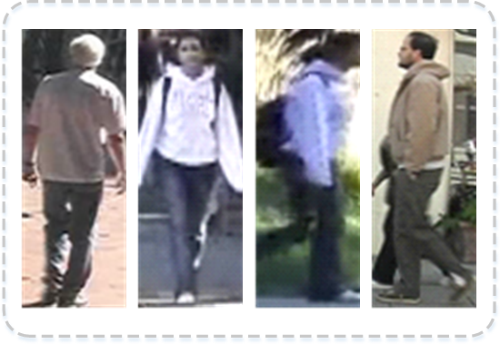
(a) Person re-identification

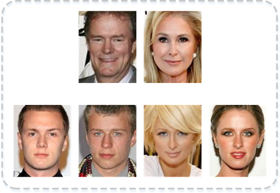
(b) Kinship verification

Figure 1: Illustration of group membership prediction (GMP) in the visual recognition tasks of (a) person re-identification and (b) kinship verification. Here we would like to predict (a) whether the four pedetrain images are taken from the same person, and (b) whether the face images are from the same family. These images are borrowed from (a) VIPeR dataset [13] and (b) Family101 dataset [8], respectively.

We introduce a novel parametric probability model for predicting group membership. Our key insight is that although the visual appearances can significantly vary, they share a set of latent variables common to all views. As depicted in Fig. 2, we can hypothesize “body parts” as shared latent variables for all the pedestrian images, while for kinship verification “facial landmarks” could be considered as the shared latent variables. Our model postulates that conditioned on the location of each shared latent variable (body part or facial landmark) the visual appearance at that location is conditionally independent for different views. This property leads to a natural way of measuring image similarities through comparison of visual similarities of the same shared latent variables across different views.

This postulate leads us to a joint parametric probability model that consists of view-specific and view-shared random variables. View-specific variables account for visual characteristics within a view while view-shared variables account for the integration of multi-view information. The group membership likelihood factorizes into a tensor product consisting of data-independent and data-dependent factors. We learn the data-independent parameters (i.e. weights) discriminatively using bilinear classifiers. Finally we marginalize these data tensors over all the dimensions with the learned weights as the group membership scores. Our experimental results on multi-camera person Re-ID and kinship verification demonstrate the good prediction performance and computational efficiency of our method.

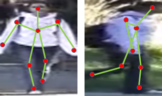
(a) Body parts

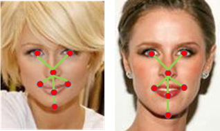
(b) Facial landmarks

Figure 2: Illustration of (a) body parts (e.g. head, torso, legs) for Re-ID and (b) facial landmarks (e.g. eyes, nose, mouth) for kinship verification. Note that in these aligned images, these body parts or facial landmarks approximately coincide in terms of spatial locations.

1.1 Related Work

GMP problem is closely related to multi-view learning (MVL). Indeed, our perspective of shared variables has been used before in the context of MVL [12, 29, 30]. Nevertheless, the goal of MVL specifically in visual recognition is different from ours. Namely, the objective of MVL is to leverage multiple sources (e.g. texts, images, videos, etc.) of data corresponding to the same underlying object (e.g. persons, events, etc.) to improve recognition performance [3, 14, 21, 30]. On the other hand our goal is to predict group membership among the multiple sources.

Person Re-ID essentially is a GMP problem, where each camera view can be taken as one of the instances. In the literature, however, most of existing works consider this problem as an independent two-view classification task, mainly focusing on cleverly designing local features [10, 20, 26, 31, 36] or learning better metrics [15, 16, 18, 19, 25, 37]. Recently, Figueira et al. [12] proposed a semi-supervised learning method to fuse multi-view features for Re-ID so that the features agree on the classification results. Das et al. [5] considered the group membership prediction in Re-ID by maximizing the summation of pairwise similarity scores using binary integer programming during testing. Unlike [5], we formulate the group membership problem as a learning problem, rather than a post-processing step to improve the matching rate.

Kinship verification is indeed another GMP problem, where each family role (e.g. father, mother, son, daughter, etc.) can be considered as an instance. Similar to person Re-ID, existing works mainly focus on learning better features [6, 9] and better distance metrics [23] for pairwise classification [22]. Recently, Qin et al. [28] proposed a bilinear model to handle so-called tri-subject kinship verification problems. Fang et al. [8] proposed a sparse group lasso based feature selection method to determine whether a query person is from a specific family. Unlike [8, 28], our method targets at a more general and challenging problem which can be used to predict an arbitrary number of images with a fixed structure of family roles, such as father-son, father-mother-daughter, grandfather-father-son-grandson, etc.

2 Our Method

2.1 Problem Setting

Let $\{(\mathcal{X}_{m},y_{m})\}_{m=1,\cdots,M}$ be a group of $M$ persons from different views, where $\forall m,\mathcal{X}_{m}$ denotes the $m^{th}$ person and $y_{m}$ denotes its label (e.g. identity or family). Let $\forall n=\{1,\cdots,N_{m}\},\mathbf{x}_{m,n}\in\mathcal{X}_{m}$ be the $n^{th}$ image for the person with $N_{m}$ images in total. The goal of our method is to predict the following probability as group membership:

$$p(y_{1}=\cdots=y_{M}|\mathcal{X}_{1},\cdots,\mathcal{X}_{M}).$$ (1)

Note that our problem setting is naturally applicable to the multiple instance cases. For example, during learning we allow multiple images to be associated with a person (i.e. $\mathcal{X}_{m}=\{\mathbf{x}_{m,n}\}$) in person Re-ID and kinship verification, as in the CUHK Campus [35] and Family101 [8] datasets.

While we have motivated our approach in the context of shared latent variables (body parts or facial landmarks), this information is unavailable during the training or testing phases. Furthermore, estimating locations of body parts and facial landmarks is known to be extremely challenging [2, 38]. Fortunately, in the context of the applications and problems that we are concerned with, the images are approximately aligned. In these images, foreground objects are centralized and well cropped. Currently most benchmark datasets are composed of such approximately aligned images, namely, the same body parts or facial landmarks appear roughly at similar locations. In such cases, pixel locations provide good approximation of where body parts and facial landmarks are, and we utilize this property to bypass the detection challenge, while accounting for spatial misalignments with spatial kernels. Note that the issue of visual ambiguity of the shared variables still remains in our problem.

2.2 Parametric GMP Model

(a) Parametric probability model

(b) Pairwise decomposition

Figure 3: (a) Graphical representation of our parametric probability model for GMP. (b) Pairwise decomposition of our model in (a).

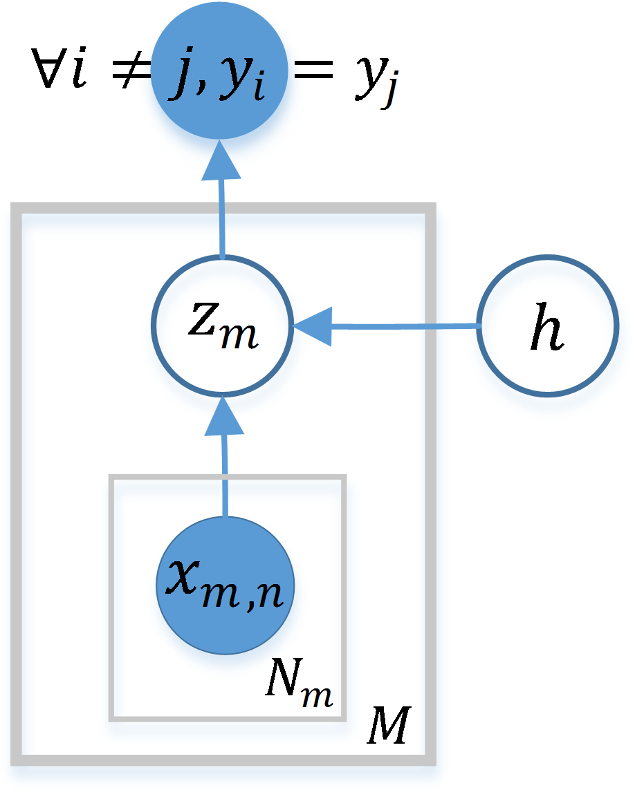
We introduce two latent variables to model the relationship between the class labels $\{y_{m}\}$ and data samples $\{\mathcal{X}_{m}\}$. The graphical representation of our parametric probability model is shown in Fig. 3(a), where $\forall m,z_{m}$ denotes the view-specific latent variable for view $m$, $h$ denotes the view-shared latent variable, and $N_{m}$ denotes the number of images from view $m$. Based on this model, we can factorize our group membership score as follows:

$$p(y_{1}=\cdots=y_{M}|\mathcal{X}_{1},\cdots,\mathcal{X}_{M})$$ (2)

$$=\sum_{z_{1},\cdots,z_{M},h}p_{y|z}\prod_{m=1}^{M}p(z_{m}|\mathcal{X}_{m},h)p(h)$$

$$=\sum_{z_{1},\cdots,z_{M},h}p_{y|z}\cdot p(h)\prod_{m=1}^{M}\left[\frac{1}{N_{m}}\sum_{n=1}^{N_{m}}p(z_{m}|\mathbf{x}_{m,n},h)\right],$$

where $p_{y|z}=p(y_{1}=\cdots=y_{M}|z_{1},\cdots,z_{M})$.

Model interpretation. To show the intuition of our parametric probability model, we consider the person Re-ID example in Fig. 2(a) in more detail. In the Re-ID problem the view-specific latent variables $\{z_{m}\}$ can be thought of as visual appearances of body parts of different persons, and the view-shared latent variable $h$ can be considered as these body parts which are shared among all the persons.

Then using Bayes rule we can expand Eq. 2. In particular, for the two-view Re-ID problem we see that the group membership score of the image pair $(\mathbf{x}_{1},y_{1})$ and $(\mathbf{x}_{2},y_{2})$ as $p(y_{1}=y_{2}|\mathbf{x}_{1},\mathbf{x}_{2})=\sum_{z_{1},z_{2},h}p(y_{1}=y_{2}|z_{1},z_{2})p(\mathbf{x}_{1}|z_{1},h)p(\mathbf{x}_{2}|z_{2},h)p(h)$. Since visual appearances in $z_{1}$ (or $z_{2}$) are posited to be independent given image $\mathbf{x}_{1}$ (or $\mathbf{x}_{2}$) and the parts $h$, we can predict whether or not $y_{1}$ is equal to $y_{2}$ (i.e. $p(y_{1}=y_{2}|\mathbf{x}_{1},\mathbf{x}_{2})$) by marginalizing the similarities of corresponding visual features of each individual part in both images (i.e. $p(\mathbf{x}_{1}|z_{1},h)$ and $p(\mathbf{x}_{2}|z_{2},h)$) with some data-independent weights (i.e. $p(y_{1}=y_{2}|z_{1},z_{2})$ and $p(h)$). Similarly for the kinship example in Fig. 2(b) we can infer the group membership score by marginalizing the corresponding landmark similarities.

We take these data-independent weights as the model parameters for prediction, which are learned discriminatively.

2.3 Discriminative Learning of Model Parameters

2.3.1 Co-occurrence Tensor Representation

As discussed in Section 2.1, images are approximately aligned in the related applications. Specifically, in person Re-ID benchmarks the head is always located at the top of images, torso in the middle, and legs at the bottom. This typical structure has been exploited in designing discriminative features [10]. Therefore, with approximately aligned images we can bypass the problem of shared variable detection and directly utilize pixel locations as surrogates for locations of body parts or facial landmarks. Note that we can still allow small spatial misalignments by designing kernels to account for spatial distortions.

Recently, Zhang et al. [32] proposed an interesting feature representation to handle visual ambiguity and spatial distortion in images for person re-id. The basic idea in their method is to capture visual ambiguity using visual words, and match them at similar locations using distance transform to handle spatial distortion. This results in a visual word co-occurrence matrix for a pair of images.

Inspired by [32], we propose a visual word co-occurrence tensor representation using $p(z_{m}|\mathbf{x}_{m,n},h)$ from multiple views to represent the group of data samples. Their proposed Gaussian kernel [32] is computationally cumbersome. Instead we design a truncated exponential function as the spatial kernel $\kappa$ with an arbitrary distance function inside to improve flexibility and computational efficiency.

Let $\boldsymbol{\pi}_{z_{m}}\in\boldsymbol{\Pi}(z_{m},\mathbf{x}_{m,n})$ be a pixel location where the corresponding pixel in image $\mathbf{x}_{m,n}$ is encoded using visual word $z_{m}$, and $\boldsymbol{\pi}_{h}$ be the pixel location with index $h$. Then we define $p(z_{m}|\mathbf{x}_{m,n},h)$ in Eq. 2 as follows:

$$p(z_{m}|\mathbf{x}_{m,n},h)\stackrel{{\scriptstyle\Delta}}{{=}}\max_{\boldsymbol{\pi}_{z_{m}}\in\boldsymbol{\Pi}(z_{m},\mathbf{x}_{m,n})}\kappa\left(\boldsymbol{\pi}_{z_{m}},\boldsymbol{\pi}_{h};\sigma_{m}\right)$$ (3)

$$=\left\{\begin{array}[]{ll}\exp\left\{-\frac{\min_{\boldsymbol{\pi}_{z_{m}}}d(\boldsymbol{\pi}_{z_{m}},\boldsymbol{\pi}_{h})}{\sigma_{m}}\right\},&\mbox{if}\;d(\boldsymbol{\pi}_{z_{m}},\boldsymbol{\pi}_{h})\leq\alpha\\ 0,&\mbox{otherwise}.\end{array}\right.$$ (6)

where $d(\cdot,\cdot)$ denotes a distance function, $\sigma_{m}\geq 0$ denotes a predefined window size parameter for view $m$, and $\alpha\geq 0$ is a predefined spatial scale parameter. Then if we take view-specific and view-shared latent variables as the dimensions in the tensor to represent the group of data, the entry at index $(z_{1},\cdots,z_{m},h)$ can be calculated as $\prod_{m=1}^{M}\left[\frac{1}{N_{m}}\sum_{n=1}^{N_{m}}p(z_{m}|\mathbf{x}_{m,n},h)\right]$.

2.3.2 General Learning Formulation

Here we introduce additional notations to simplify our exposition. Rather than directly representing a group of data samples $\mathcal{X}_{1,\cdots,M}=\{\mathcal{X}_{1},\cdots,\mathcal{X}_{M}\}$ as a tensor, we convert it into a matrix $\phi(\mathcal{X}_{1,\cdots,M})\in\mathbb{R}^{\prod_{m=1}^{M}|z_{m}|\times|h|}$ with dimensions $\prod_{m=1}^{M}|z_{m}|$ and $|h|$, respectively, where $\forall m,|z_{m}|$ and $|h|$ denote the numbers of visual words for view $m$ and pixel locations in images. Further, we denote $\mathbf{w}_{z}\stackrel{{\scriptstyle\Delta}}{{=}}p(y_{1}=\cdots=y_{M}|z_{1},\cdots,z_{M})\in\mathbb{R}^{\prod_{m=1}^{M}|z_{m}|}$ and $\mathbf{w}_{h}\stackrel{{\scriptstyle\Delta}}{{=}}p(h)\in\mathbb{R}^{|h|}$ as our model parameters in the form of vectors. Then our group membership score in Eq. 2 can be rewritten as a decision function $f$ as follows:

$$f(\mathcal{X}_{1,\cdots,M})=\mathbf{w}_{z}^{T}\phi(\mathcal{X}_{1,\cdots,M})\mathbf{w}_{h},$$ (7)

where $(\cdot)^{T}$ denotes the matrix transpose operator. If $f(\mathcal{X}_{1,\cdots,M})\geq 0$, we expect that all the members in the group have the same class label (and do not otherwise).

Let $\{(\mathcal{X}_{1,\cdots,M}^{(k)},y_{1,\cdots,M}^{(k)})\}_{k=1,\cdots,N}$ be a set of $N$ training data groups from $M$ views, where $\forall k,y_{1,\cdots,M}^{(k)}=1$ if all the class labels in group $k$ are the same (and $-1$ otherwise). Due to the specific form in Eq. 7, we propose learning bilinear classifiers (i.e. $\mathbf{w}_{z}$ and $\mathbf{w}_{h}$) for GMP inspired by [27], which used bilinear classifiers in a different context (binary classification):

$$\min_{\mathbf{w}_{z},\mathbf{w}_{h}}\frac{\lambda_{1}}{2}\|\mathbf{w}_{z}\|_{2}^{2}+\frac{\lambda_{2}}{2}\|\mathbf{w}_{h}\|_{2}^{2}+\sum_{k=1}^{N}\ell\left(y_{1,\cdots,M}^{(k)},f(\mathcal{X}_{1,\cdots,M}^{(k)})\right),$$ (8)

where $\ell(\cdot,\cdot)$ denotes the loss function (e.g. hinge loss), $\lambda_{1}\geq 0,\lambda_{2}\geq 0$ are predefined regularization parameters, and $\|\cdot\|_{2}$ denotes the $\ell_{2}$-norm of a vector.

Note that here we relax the probability constraint on $\mathbf{w}_{z}$ and $\mathbf{w}_{h}$ to real numbers so that Eq. 8 can be efficiently solved using alternating optimization. In each iteration, we fix one parameter (i.e. $\mathbf{w}_{z}$ or $\mathbf{w}_{h}$) and use a standard support vector machine (SVM) solver to find the other parameter so that the objective value decreases monotonically, thus guaranteeing a local optimal solution.

2.3.3 Pairwise Decomposition Approximation

With sufficient training data, we can train a bilinear classifier directly using Eq. 8. This training method, however, does not scale well with the number of views due to the high dimensional tensor representation, leading to serious computational and overfitting issues.

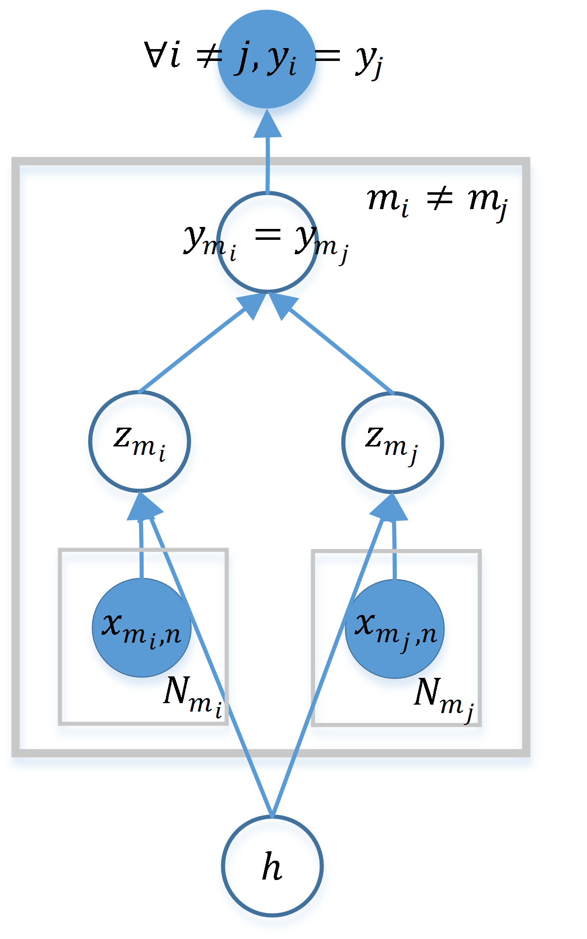
To overcome these issues, we propose an approximate pairwise decomposition method, as illustrated in Fig. 3(b), to reduce the parameter space. This is based on the conditional independence assumption in multi-view learning [1]. Accordingly, we can rewrite our group membership score in Eq. 2 as follows:

$$p(y_{1}=\cdots=y_{M}|\mathcal{X}_{1},\cdots,\mathcal{X}_{M})$$ (9)

$$\equiv\sum_{m_{i}\neq m_{j}\in\{1,\cdots,M\}}\sum_{z_{m_{i}},z_{m_{j}},h}p(y_{1}=\cdots=y_{M}|y_{m_{i}}=y_{m_{j}})$$

$$p(y_{m_{i}}=y_{m_{j}}|z_{m_{i}},z_{m_{j}})p(z_{m_{i}}|\mathcal{X}_{m_{i}},h)p(z_{m_{j}}|\mathcal{X}_{m_{j}},h)p(h).$$

where $p(y_{1}=\cdots=y_{M}|y_{m_{i}}=y_{m_{j}})$ indicates how importantly the pair of views $m_{i}$ and $m_{j}$ contribute to GMP. In this way, the number of parameters that need to be learned in our method is significantly reduced from $\left(\prod_{m=1}^{M}|z_{m}|+|h|\right)$ to $\left(\sum_{m_{i}\neq m_{j}}|z_{m_{i}}||z_{m_{j}}|+|h|\right)$.

Let $\phi(\mathcal{X}_{m_{i},m_{j}})\stackrel{{\scriptstyle\Delta}}{{=}}p(z_{m_{i}}|\mathcal{X}_{m_{i}},h)p(z_{m_{j}}|\mathcal{X}_{m_{j}},h)\in\mathbb{R}^{(|z_{m_{i}}||z_{m_{j}}|)\times|h|}$ be the pairwise visual word matrix between views $m_{i}$ and $m_{j}$, where $\mathcal{X}_{m_{i},m_{j}}=\{\mathcal{X}_{m_{i}},\mathcal{X}_{m_{j}}\}$. Also let $\mathbf{w}_{m_{i},m_{j}}\stackrel{{\scriptstyle\Delta}}{{=}}p(y_{m_{i}}=y_{m_{j}}|z_{m_{i}},z_{m_{j}})\in\mathbb{R}^{|z_{m_{i}}||z_{m_{j}}|}$ , and $\boldsymbol{\beta}\stackrel{{\scriptstyle\Delta}}{{=}}p(y_{1}=\cdots=y_{M}|y_{m_{i}}=y_{m_{j}})\in\mathbb{R}^{|z_{m_{i}}||z_{m_{j}}|}$ . Then based on Eq. 9, we can rewrite Eq. 7 as follows:

$$\tilde{f}(\mathcal{X}_{1,\cdots,M})=\sum_{m_{i}\neq m_{j}}\beta_{m_{i},m_{j}}\mathbf{w}_{m_{i},m_{j}}^{T}\phi(\mathcal{X}_{m_{i},m_{j}})\mathbf{w}_{h},$$ (10)

where $\beta_{m_{i},m_{j}}$ denotes the entry in $\boldsymbol{\beta}$ for the view pair.

Input : $\{\phi(\mathcal{X}_{m_{i},m_{j}})\}_{\forall m_{i}\neq m_{j}\in\{1,...,M\}}$, $\{y_{m_{i}}\}_{\forall m_{i}\in{1,...,M}}$, $\lambda_{1},\lambda_{2},\lambda_{3}\geq 0$ Output : $\{\mathbf{w}_{m_{i},m_{j}}\}_{m_{i}\neq m_{j}\in\{1,...,M\}},\mathbf{w}_{h},\boldsymbol{\beta}$ Initialize $\boldsymbol{\beta}\leftarrow\mathbf{1}$, $\mathbf{w}_{h}\leftarrow\mathbf{1}$, $\mathbf{w}_{m_{i},m_{j}}\leftarrow\mathbf{1}$;

repeat

  Solve $\{\mathbf{w}_{m_{i},m_{j}}\}$ in Eq. 11 (multi-view training) or Eq. 12 (double-view training) by fixing $\boldsymbol{\beta}$ and $\mathbf{w}_{h}$;

Solve $\mathbf{w}_{h}$ in Eq. 11 or Eq. 12 by fixing $\boldsymbol{\beta}$ and $\{\mathbf{w}_{m_{i},m_{j}}\}$ ;

Solve $\boldsymbol{\beta}$ in Eq. 11 or Eq. 12 by fixing $\{\mathbf{w}_{m_{i},m_{j}}\}$ and $\mathbf{w}_{h}$. until Converge;

return $\{\mathbf{w}_{m_{i},m_{j}}\}_{m_{i}\neq m_{j}\in\{1,...,M\}},\mathbf{w}_{h},\boldsymbol{\beta}$;

Algorithm 1 Pairwise decomposition based learning

To learn our model parameters in Eq. 10, we propose two learning methods as follows, namely, multi-view training and double-view training:

Multi-view training:

$$\min_{\begin{subarray}{c}\{\mathbf{w}_{m_{i},m_{j}}\},\\ \mathbf{w}_{h},\boldsymbol{\beta}\end{subarray}}\frac{\lambda_{1}}{2}\sum_{m_{i}\neq m_{j}}\|\mathbf{w}_{m_{i},m_{j}}\|_{2}^{2}+\frac{\lambda_{2}}{2}\|\mathbf{w}_{h}\|_{2}^{2}+\frac{\lambda_{3}}{2}\|\boldsymbol{\beta}\|_{2}^{2}$$

$$+\sum_{k=1}^{N}\ell\left(y_{1,\cdots,M}^{(k)},\tilde{f}(\mathcal{X}_{1,\cdots,M}^{(k)})\right),\;\;\mbox{s.t.}\;\boldsymbol{\beta}\geq\mathbf{0},$$ (11)

Double-view training:

$$\min_{\begin{subarray}{c}\{\mathbf{w}_{m_{i},m_{j}}\},\\ \mathbf{w}_{h},\boldsymbol{\beta}\end{subarray}}\frac{\lambda_{1}}{2}\sum_{m_{i}\neq m_{j}}\|\mathbf{w}_{m_{i},m_{j}}\|_{2}^{2}+\frac{\lambda_{2}}{2}\|\mathbf{w}_{h}\|_{2}^{2}+\frac{\lambda_{3}}{2}\|\boldsymbol{\beta}\|_{2}^{2}$$

$$+\sum_{k=1}^{N}\sum_{m_{i}\neq m_{j}}\ell\left(y_{m_{i},m_{j}}^{(k)},\tilde{f}(\mathcal{X}_{m_{i},m_{j}}^{(k)})\right),\;\;\mbox{s.t.}\;\boldsymbol{\beta}\geq\mathbf{0},$$ (12)

where $\forall k,y_{m_{i},m_{j}}^{(k)}=1$ if in group $k$ the labels of the two persons $y_{m_{i}}=y_{m_{j}}$ holds; otherwise, 0. Here, $\geq$ denotes an element-wise $\geq$ operator. Both training can be done using alternating optimization with a standard SVM solver. Still local optima are guaranteed. For two-view scenarios, both training methods are essentially identical, and scale quadratically with the number of views, in general. Linear scalability is also possible if we organize all the views as cycle graphs. Difference in these two training methods comes from the loss functions, where in multi-view training $\ell$ measures the group (i.e. multi-view) loss, while in double-view training $\ell$ measures the pair-view loss. Our algorithm is summarized in Alg. 1.

(a)

(b)

Figure 4: CMC curve comparison on (a) VIPeR and (b) CUHK01, respectively. Notice that except our results, the rest are copied from [36].

3 Experiments

We evaluate our method on person Re-ID and kinship verification tasks along with state-of-the-art methods on benchmark datasets. Standard training/testing protocols are used in all experiments. For each comparing method, we either cite the original results from the papers (denoted by $(\cdot)^{*}$ in the tables) or calculate from released codes. Our results are reported as the average over 3 trials.

For each experiment, we choose the same or similar low-level feature as the other methods (see the details in subsection) for fair comparison. We densely sample the images to generate a low-level local feature per pixel. Then we use K-Means to build the visual vocabularies with about $2\times 10^{4}$ randomly selected features per view. Further, every local feature is quantized into one of these visual words based on Euclidean distance. Note that more complicated feature selection methods may be employed to yield better performance, but we do not fine-tune this component for the sake of computational efficiency and generalization ability.

We employ the chessboard distance for Eq. 3 and LIBLINEAR [7] as our SVM solver with hinge loss. We randomly generate about $3\times 10^{4}$ training samples to learn model parameters $\mathbf{w}$’s. The regularization parameters are determined by cross-validation.

3.1 Person Re-identification

For performance measure we adopt the standard Cumulative Match Characteristic (CMC) curve, which displays the recognition rate as a function of rank. The recognition rate at rank-$r$ is the proportion of queries correctly matched to a corresponding gallery entity at rank-$r$ or better.

For tasks with multiple camera views, we follow [5] to compare results under two camera views. Consider the results from multiple views as a high dimensional tensor, one dimension per view. To predict pairwise matches from multi-view results (e.g. identifying matches between camera view 1 and view 2 from the predicted results for the joint of view 1, 2, and 3), we can either sum over or find the maximum over the extra dimensions. Cross-validation is used to choose the better way for each dataset.

3.1.1 Two Camera Views

Table 1: Matching rate comparison (%) on VIPeR and CUHK01.

Rank $r=$	1	5	10	15	20	25
	VIPeR
SCNCD [31]	20.7	47.2	60.6	68.8	75.1	79.1
SCNCDfinal [31]	37.8	68.5	81.2	87.0	90.4	92.7
LADF [19]	29.3	61.0	76.0	83.4	88.1	90.9
Mid-level filters [36]	29.1	52.3	65.9	73.9	79.9	84.3
Mid-level+LADF [36]	43.4	73.0	84.9	90.9	93.7	95.5
VW-CooC [32]	30.70	62.98	75.95	81.01	-	-
Ours	33.5	59.5	72.8	81.3	88.0	89.6
	CUHK01
Single-shot LAFT∗ [18]	25.8	55.0	66.7	73.8	79.0	83.0
Multi-shot LAFT∗ [18]	31.4	58.0	68.3	74.0	79.0	83.0
Mid-level filters [36]	34.3	55.1	65.0	71.0	74.9	78.0
VW-CooC [32]	44.03	70.47	79.12	84.77	-	-
Ours	60.39	82.92	90.43	93.42	94.55	95.78

Person Re-ID between two views is the simplest scenario. We test our method on the VIPeR [13] and CUHK Campus [35] dataset. We extract a 672-dim Color+SIFT vector from each 5$\times$5 pixel patch in images as low-level features. We follow the experimental setting in [35] for both datasets.

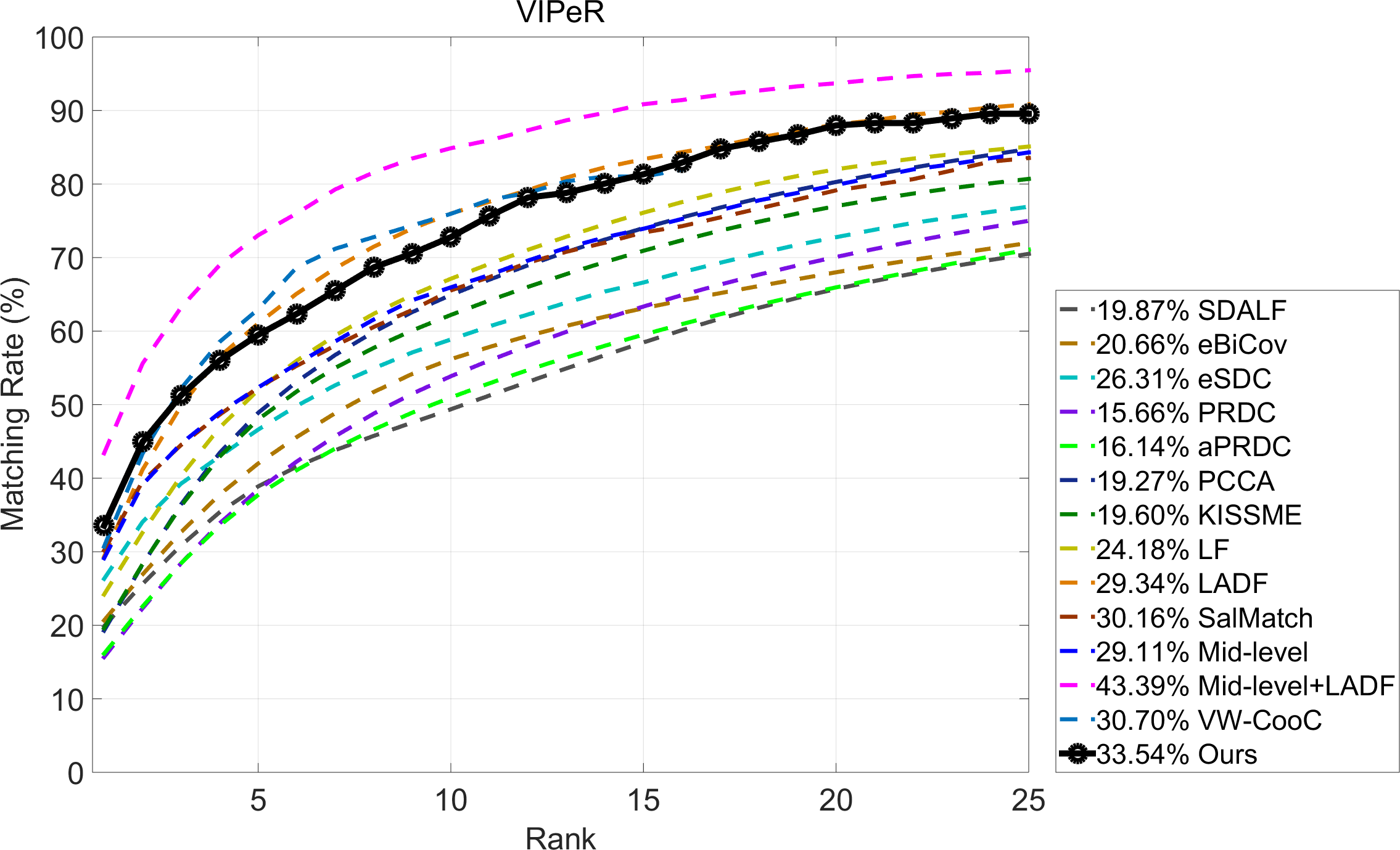
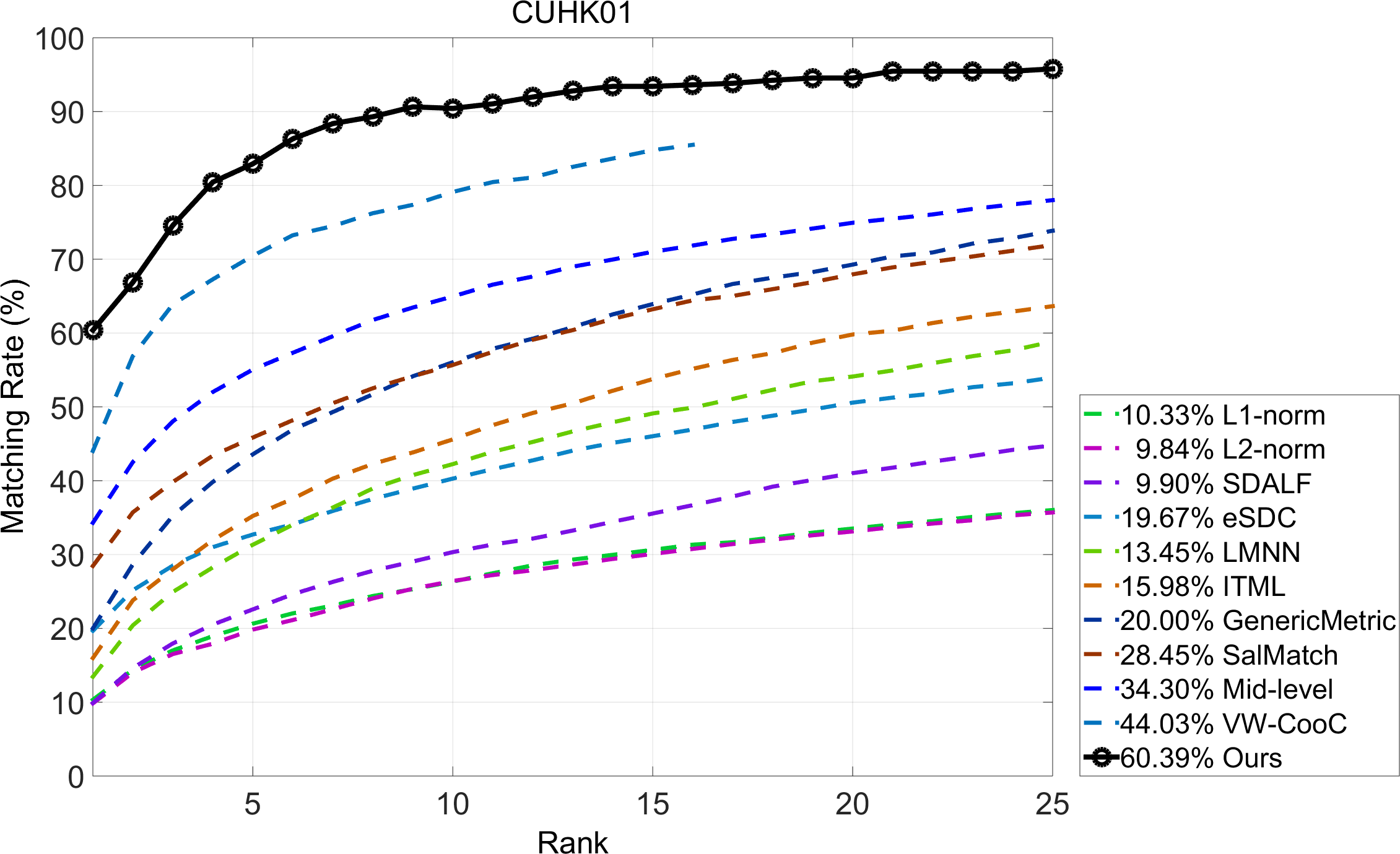
Our comparison results are listed in Table 1. As we see, on VIPeR “Mid-level+LADF” from [36] is the current best method, which utilized more discriminative mid-level filters as features and a powerful classifier, and “SCNCD_final” from [31] is the second, which utilized only foreground features. Our results are comparable to both of them. However, our method always outperforms their original methods significantly when either the powerful classifier or the foreground information is not involved. On CUHK01, our method performs the best. At rank-1, it outperforms [32, 36] by 16.36% and 26.09%, respectively. Compared with [32], the improvement mainly comes from the multiple instance setting of our method.

The CMC curve comparison on VIPeR and CUHK01 is shown in Fig. 4. As we see, our curve is very similar to that of LADF. This is mainly because LADF is a second-order (i.e. quadratic) decision function based on metric learning, which shares some commonality with our classifiers.

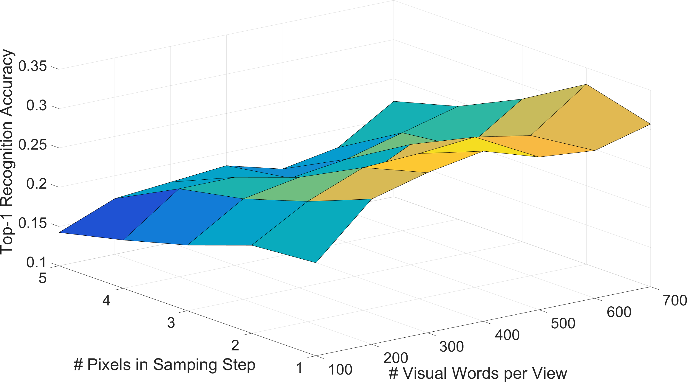
We also demonstrate the impacts of different numbers of pixel locations (i.e. view-shared space) and visual words (i.e. view-specific space) on the performance using VIPeR in Fig. 5. We sample the pixel locations, step by from 1 to 5 pixels along x and y-axis in images (larger number leading to fewer samples), while using different numbers of visual words. Visual words capture the variations in appearance, and with more visual words more similar patterns can be differentiated (e.g. pink and red). Matching between pixel locations gives us the statistic information of visual words, and more samples make the statistics more robust. Together they work for good performance.

Figure 5: Demonstration of the impacts of different numbers of pixel locations and visual words on the performance using VIPeR. Warmer color demotes higher accuracy. This figure is best viewed in color.

Figure 6: CMC curve comparison on WARD. Note except for our results, the other results are cited from [5].

3.1.2 Three Camera Views

Now we consider three camera views, and test our method on the WARD dataset [24]. Following [5], we denote the camera views as view 1, 2 and 3. However, for pairwise view matching, [5] did not mention which view as probe or gallery. Here, we define the view with a smaller/larger number of data to be the gallery/probe set. We randomly select 35 people for training, and the rest for testing.

We first resize each image to the same $128\times 64$ pixels, and take every $2\times 2$ pixel patch in the HSV color space to generate our low-level features by concatenating $3\times 2\times 2=12$ entries into a vector. The reason for choosing this feature is because in [5] the features were built in the HSV color space as well. Different from [5], we take the whole image to generate features without foreground segmentation.

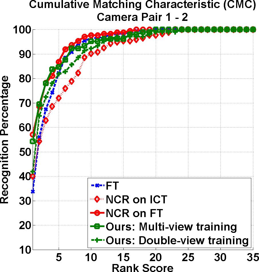
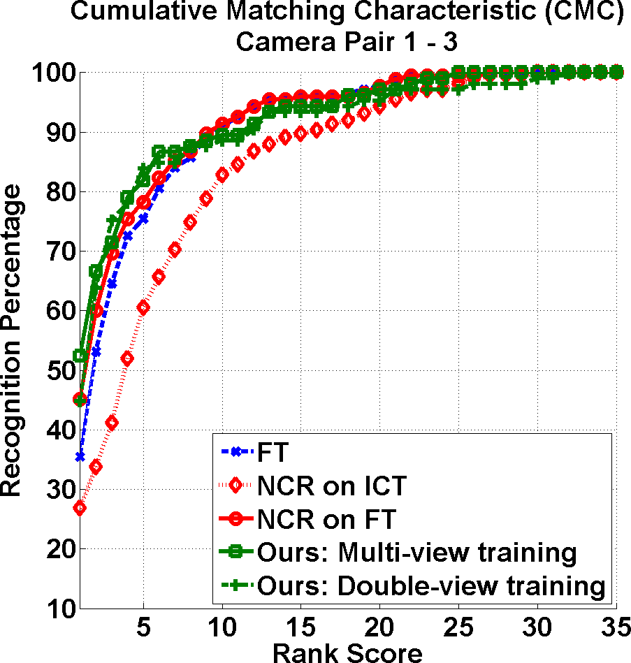
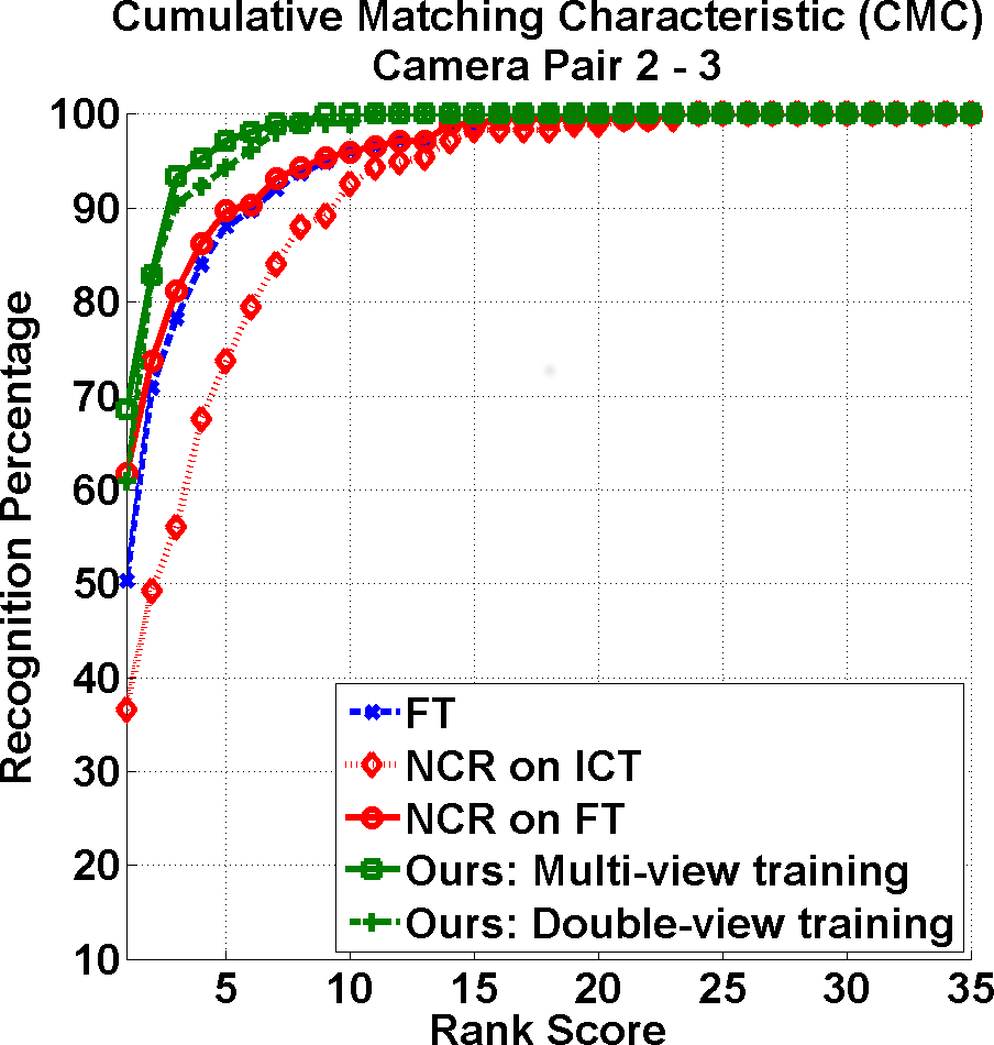
The results are shown in Fig. 6. As we see, our method performs similar or better than NCR [5], and the curves of both the multi-view training and double-view training for our method behave very similarly. We list the area under curve (AUC) scores in Table 2. Our method is better than NCR on FT by 0.6%, on average, from 94.3% to 94.9%.

Table 2: AUC comparison (%) on WARD based on Fig. 6.

View pair	1-2	1-3	2-3	Ave.
FT	93.3	91.0	94.9	93.1
NCR on ICT	90.4	84.8	91.1	88.7
NCR on FT	95.4	91.9	95.6	94.3
Ours: Multi-view	94.4	92.1	98.1	94.9
Ours: Double-view	92.7	91.0	97.5	93.8

Figure 7: CMC curve comparison on RAiD. Notice that expect our results, the rest results are cited from [5].

3.1.3 Four Camera Views

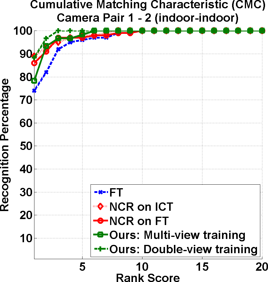
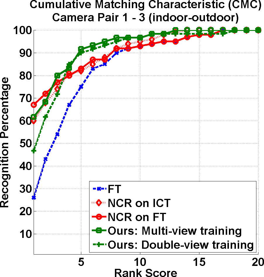
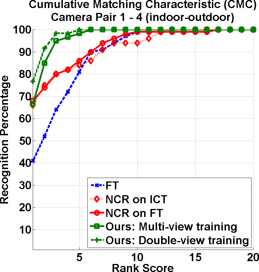
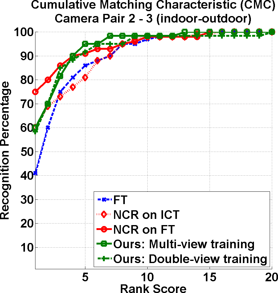
Next we consider four camera views, and test our method on the Re-identification Across indoor-outdoor Dataset (RAiD) [5] with two indoor views camera 1 and 2, and two outdoor views camera 3 and 4. Still we take the views with smaller/larger numbers as galleries/probes. We follow [5], and utilize the same HSV low-level feature as we did in Section 3.1.2.

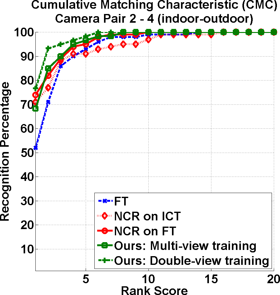
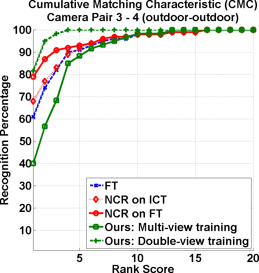
Our comparison results are shown in Fig. 7. As we see, our method again performs equally well or better than NCR. We list the AUC score comparison results in Table 3. Still our method is better than NCR on FT by 1.6%, on average, from 94.7% to 96.3%.

For both indoor-indoor and outdoor-outdoor cases, our method consistently works best, which may indicate that the visual word co-occurrence patterns are more discriminative if the lighting condition is similar.

Table 3: AUC comparison (%) on RAiD based on Fig. 7.

View pair	1-2	1-3	1-4	2-3	2-4	3-4	Ave.
FT	96.6	84.3	88.8	90.0	93.9	93.5	91.2
NCR on ICT	98.5	90.6	92.1	91.0	94.4	94.1	93.4
NCR on FT	98.1	90.4	93.1	94.5	96.5	95.9	94.7
Ours: Multi-view	98.2	93.0	97.1	94.1	96.6	90.5	94.9
Ours: Double-view	99.3	90.8	98.3	93.0	98.0	98.8	96.3

3.2 Kinship Verification & Identification

As before, we utilize the HSV 12-dim low-level features. In the experiments, we denote father, mother, son, and daughter as F, M, S, and D, respectively. Following [23], we measure the verification performance with the verification rate, defined by the number of correctly classified face pairs divided by the total number of face pairs in the test set. For identification, CMC curves are also used. We only use double-view training in this task since the information captured by parent-offspring pairs are more important.

Kinship verification between two views (one parent and one offspring) is the conventional setting, where we test our method on two datasets, i.e. KinFaceW-I [23] and KinFaceW-II [23]. The former consists of 156 FS, 134 FD, 116 MS and 127 MD pairs, while the latter contains 250 pairs of each kin relation. The main difference between the two datasets is that each pair of face images in KinFaceW-II comes from the same photo while the image pairs in KinFace-I come from different photos. We follow the same protocol as that in [23, 6, 28] and use a 5-fold cross validation with balanced positive and negative pairs on the default training/testing split. Results are listed in Table 4.

On KinFaceW-II, our method significantly outperforms the competitors, but on KinFaceW-I ours is slightly worse. Our reasoning is that our current visual word representation using simple K-Means does not account for significant visual ambiguity in appearance when imaging factors (e.g. lighting conditions, illumination, etc.) change substantially. This leads to large intra-cluster variations in visual words that our method does not currently handle well. To further investigate the different performances on both datasets, we use a smaller training set randomly sampled on KinFaceW-II such that it has the same size as KinFaceW-I, while keeping the same test set and record the results as “reduced training set”. The results become slightly worse than the original training set, while still outperform other methods. These relatively good results, along with the worse results on KinFaceW-I, demonstrate that the size of training data is indeed important, but less important than the data sources.

Table 4: Verification rate comparison (%) on KinFaceW

•	FS	FD	MS	MD	Mean
	KinFaceW-I
Dehghan et al. [6]	76.4	72.5	71.9	77.3	74.5
Lu et al. [23]	72.5	66.5	66.2	72.0	69.9
Qin et al. [28]	76.8	76.8	74.6	78.0	76.6
Ours	63.5	65.0	63.8	75.6	67.0
	KinFaceW-II
Dehghan et al. [6]	83.9	76.7	83.4	84.8	82.2
Lu et al. [23]	76.9	74.3	77.4	77.6	76.5
Qin et al. [28]	84.6	77.0	84.4	85.4	82.9
Ours	85.4	81.8	86.6	90.0	86.0
Ours (reduced training set)	84.4	78.2	84.6	87.8	83.8

Next we use TSKinFace dataset [28] for three-view kinship verification (i.e. father, mother, offspring), which contains 513 FM-S and 502 FM-D groups. Following [28], we carry out a 5-fold cross validation with balanced positive and negative samples , and list the results in Table 5. As we see, our method performs consistently better than [28].

Table 5: Verification rate comparison (%) on TSKinFace.

	FS	FD	MS	MD	FM-S	FM-D
Dehghan et al. [6]	79.9	74.2	78.5	76.3	81.9	79.6
Fang et al. [8]	69.1	66.8	68.7	67.9	71.6	69.8
Lu et al. [23]	74.8	70.0	72.2	71.3	77.0	71.4
Qin et al. [28]	83.0	80.5	82.8	81.1	86.4	84.4
Ours	88.5	87.0	87.9	87.8	90.6	89.0

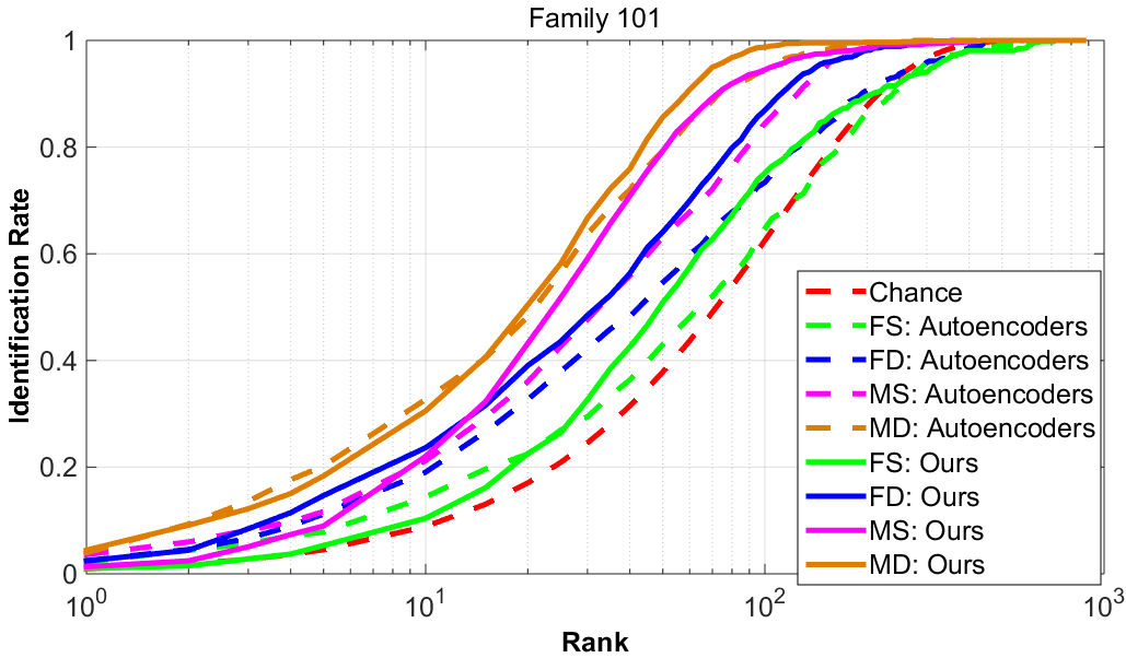
Finally we employ the Family 101 dataset [8] to investigate kinship identification, namely, identifying the correct parent/child among a set of candidates given one child/parent image. This dataset contains 14816 images that form 206 nuclear families belonging to 101 unique family trees. Following [6], we adopt 101 nuclear families and use 50 families for training and 51 families for testing. For each of the four kin relations, we train a model and use the model to match offspring images to all possible parent images. The CMC curves are shown in Fig. 8 , and Table 6 lists the Area Under Curve (AUC) measure of the CMC curves.

Table 6: AUC comparison (%) on Family 101.

•	FS	FD	MS	MD	Mean
Dehghan et al. [6]	88.8	91.3	94.3	96.4	92.7
Ours	90.3	94.6	96.0	97.0	94.5

Figure 8: CMC curve comparison with [6] on Family 101.

3.3 Storage & Computational Time

Storage ($S_{t}$ for short) and computational time during testing are two critical issues in real-world applications. In our method, we only need to store a feature matrix for each entity based on Eq. 3, which is used to calculate similarities between different entities. The computational time can be roughly divided into two parts: (1) computing feature matrices $T_{1}$, and (2) predicting group membership $T_{2}$. We do not consider the time for generating low-level features, since different implementations vary significantly.

We record the storage and computational time using 300 visual words for both probe and gallery sets on VIPeR (two views), WARD (three views), and RAiD (four views). The rest of the parameters are the same as described in Section 3.1. As we see, the storage per data sample and computational time are linearly proportional to the size of images and number of visual words. Our implementation is based on unoptimized MATLAB code. Numbers are listed in Table 7, including the time for saving and loading features. Our experiments were all run on a multi-thread CPU (Xeon E5-2696 v2) with a GPU (GTX TITAN). The method runs efficiently with very low demand for storage.

Table 7: Average storage and computational time for our mdthod.

	$S_{t}$ (Kb)	$T_{1}$ (ms)	$T_{2}$ (ms)
VIPeR	110.7	52.9	0.6
WARD	113.7	99.7	1.5
RAiD	166.5	68.7	0.5

4 Conclusion

In this paper, we propose a general parametric probability model for the group membership prediction (GMP) problem. We introduce the notions of view-specific and view-shared latent variables to capture visual information and commonality for each view. Using these two variables, we can factorize the group membership score into a tensor product, and thus propose a new visual word co-occurrence tensor feature to represent groups of data samples. In our parametric probability model, we can handle the multiple instance cases as well. Further we propose discriminatively learning a bilinear classifier for GMP, with the decision function as the marginalization over all latent variables. Our experiments on multi-camera person re-id and kinship verification tasks demonstrate the good predictive ability and computational efficiency of our method. As future work, we would like to explore other applications for our method such as activity retrieval [4], and develop new approaches such as zero-shot recognition [34] and structured learning [33] for our problem.

References

- [1] A. Blum and T. Mitchell. Combining labeled and unlabeled data with co-training. In COLT, pages 92–100, 1998.
- [2] L. Bourdev and J. Malik. Poselets: Body part detectors trained using 3d human pose annotations. In CVPR, pages 1365–1372, 2009.
- [3] Z. Cai, L. Wang, X. Peng, and Y. Qiao. Multi-view super vector for action recognition. In CVPR, pages 596–603, 2014.
- [4] G. D. Castanon, Y. Chen, Z. Zhang, and V. Saligrama. Efficient activity retrieval through semantic graph queries. In ACM Multimedia, 2015.
- [5] A. Das, A. Chakraborty, and A. K. Roy-Chowdhury. Consistent re-identification in a camera network. In ECCV, pages 330–345, 2014.
- [6] A. Dehghan, E. G. Ortiz, R. Villegas, and M. Shah. Who do i look like? determining parent-offspring resemblance via gated autoencoders. In CVPR, pages 1757–1764, 2014.
- [7] R.-E. Fan, K.-W. Chang, C.-J. Hsieh, X.-R. Wang, and C.-J. Lin. LIBLINEAR: A library for large linear classification. JMLR, 9:1871–1874, 2008.
- [8] R. Fang, A. C. Gallagher, T. Chen, and A. C. Loui. Kinship classification by modeling facial feature heredity. In ICIP, pages 2983–2987, 2013.
- [9] R. Fang, K. D. Tang, N. Snavely, and T. Chen. Towards computational models of kinship verification. In ICIP, pages 1577–1580, 2010.
- [10] M. Farenzena, L. Bazzani, A. Perina, V. Murino, and M. Cristani. Person re-identification by symmetry-driven accumulation of local features. In CVPR, pages 2360–2367, 2010.
- [11] P. F. Felzenszwalb, R. B. Girshick, D. McAllester, and D. Ramanan. Object detection with discriminatively trained part based models. PAMI, 32(9):1627–1645, 2010.
- [12] D. Figueira, L. Bazzani, H. Q. Minh, M. Cristani, A. Bernardino, and V. Murino. Semi-supervised multi-feature learning for person re-identification. In AVSS, pages 111–116, 2013.
- [13] D. Gray, S. Brennan, and H. Tao. Evaluating appearance models for recognition, reacquisition, and tracking. In PETS, pages 41–47, 2007.
- [14] M. M. Kalayeh, H. Idrees, and M. Shah. Nmf-knn: Image annotation using weighted multi-view non-negative matrix factorization. In CVPR, 2014.
- [15] S. Khamis, C.-H. Kuo, V. K. Singh, V. Shet, and L. S. Davis. Joint learning for attribute-consistent person re-identification. In ECCV Workshop on Visual Surveillance and Re-Identification, pages 134–146, 2014.
- [16] M. Kostinger, M. Hirzer, P. Wohlhart, P. Roth, and H. Bischof. Large scale metric learning from equivalence constraints. In CVPR, pages 2288–2295, 2012.
- [17] L.-J. Li, R. Socher, and F.-F. Li. Towards total scene understanding: Classification, annotation and segmentation in an automatic framework. In CVPR, pages 2036–2043, 2009.
- [18] W. Li and X. Wang. Locally aligned feature transforms across views. In CVPR, pages 3594–3601, 2013.
- [19] Z. Li, S. Chang, F. Liang, T. S. Huang, L. Cao, and J. R. Smith. Learning locally-adaptive decision functions for person verification. In CVPR, pages 3610–3617, 2013.
- [20] C. Liu, S. Gong, C. C. Loy, and X. Lin. Person re-identification: what features are important? In ECCV, pages 391–401, 2012.
- [21] J. Liu, Y. Jiang, Z. Li, Z.-H. Zhou, and H. Lu. Partially shared latent factor learning with multiview data. NNLS, 2014.
- [22] J. Lu, J. Hu, V. E. Liong, X. Zhou, A. Bottino, I. U. Islam, T. F. Vieira, X. Qin, X. Tan, Y. Keller, et al. The fg 2015 kinship verification in the wild evaluation. In FG, 2015.
- [23] J. Lu, X. Zhou, Y.-P. Tan, Y. Shang, and J. Zhou. Neighborhood repulsed metric learning for kinship verification. PAMI, 36(2):331–345, 2014.
- [24] N. Martinel and C. Micheloni. Re-identify people in wide area camera network. In CVPR Workshops, pages 31–36, 2012.
- [25] A. Mignon and F. Jurie. PCCA: a new approach for distance learning from sparse pairwise constraints. In CVPR, pages 2666–2672, 2012.
- [26] S. Pedagadi, J. Orwell, S. Velastin, and B. Boghossian. Local fisher discriminant analysis for pedestrian re-identification. In CVPR, pages 3318–3325, 2013.
- [27] H. Pirsiavash, D. Ramanan, and C. Fowlkes. Bilinear classifiers for visual recognition. In NIPS, pages 1482–1490, 2009.
- [28] X. Qin, X. Tan, and S. Chen. Tri-subject kinship verification: Understanding the core of a family. arXiv:1501.02555, 2015.
- [29] Y. Song, L.-P. Morency, and R. Davis. Multi-view latent variable discriminative models for action recognition. In CVPR, pages 2120–2127, 2012.
- [30] C. Xu, D. Tao, and C. Xu. A survey on multi-view learning. arXiv:1304.5634, 2013.
- [31] Y. Yang, J. Yang, J. Yan, S. Liao, D. Yi, and S. Z. Li. Salient color names for person re-identification. In ECCV, pages 536–551, 2014.
- [32] Z. Zhang, Y. Chen, and V. Saligrama. A novel visual word co-occurrence model for person re-identification. In ECCV Workshop on Visual Surveillance and Re-Identification, pages 122–133, 2014.
- [33] Z. Zhang and V. Saligrama. PRISM: Person re-identification via structured matching. arXiv preprint arXiv:1406.4444, 2014.
- [34] Z. Zhang and V. Saligrama. Zero-shot learning via semantic similarity embedding. In ICCV, 2015.
- [35] R. Zhao, W. Ouyang, and X. Wang. Person re-identification by salience matching. In ICCV, pages 2528–2535, 2013.
- [36] R. Zhao, W. Ouyang, and X. Wang. Learning mid-level filters for person re-identification. In CVPR, pages 144–151, 2014.
- [37] W.-S. Zheng, S. Gong, and T. Xiang. Re-identification by relative distance comparison. PAMI, 35(3):653–668, 2013.
- [38] X. Zhu and D. Ramanan. Face detection, pose estimation, and landmark localization in the wild. In CVPR, pages 2879–2886, 2012.