Diffusion Processes Homogenization for Scale-Free Metric Networks

Abstract

This work discusses the homogenization analysis for diffusion processes on scale-free metric graphs, using weak variational formulations. The oscillations of the diffusion coefficient along the edges of a metric graph induce internal singularities in the global system which, together with the high complexity of large networks constitute significant difficulties in the direct analysis of the problem. At the same time, these facts also suggest homogenization as a viable approach for modeling the global behavior of the problem. To that end, we study the asymptotic behavior of a sequence of boundary problems defined on a nested collection of metric graphs. This paper presents the weak variational formulation of the problems, the convergence analysis of the solutions and some numerical experiments.

1 Introduction

A scale-free network is a large graph with power law degree distribution, i.e., $\operatorname*{\bm{\mathbbm{P}}}[\deg(v)=k]\sim k^{-\gamma}$ where $\gamma$ is a fixed positive constant. Equivalently, the probability of finding a vertex of degree $k$, decays as a power-law of the degree value. Power-law distributed networks are of noticeable interest because they have been frequently observed in very different fields such as the World Wide Web, business networks, neuroscience, genetics, economics, etc. The current research on scale-free networks is mainly focused in three aspects: first, generation models (see [1, 2]), second, solid evidence detection of networks with power-law degree distribution (see [3, 4, 5, 6]). The third and final aspect studies the extent to which the power-law distribution relates with other structural properties of the network, such as self-organization (see [7, 8]); this is subject of intense debate, see [7] for a comprehensive survey on the matter.

The present work studies scale-free networks from a very different perspective. Its main goal is to introduce a homogenization process on the network, aimed reduce the original order of complexity but preserving the essential features (see Figure 1). In this way, the “homogenized” or “upscaled” network is reliable for data analysis while, at the same time, involves lower computational costs and lower numerical instability. Additionally, the homogenization process derives a neater and more structural picture of the starting network since unnecessary complexity is replaced by the average asymptotic behavior of large data. The phenomenon known as “The Aggregation Problem” in economics is an example of how this type of reasoning is implicitly applied in modeling the global behavior of large networks (see [9]). Usually, homogenization techniques require some assumptions of periodicity of the singularities or the coefficients of the system (see [10, 11]), in turn this case demands averaging hypotheses in the Cesàro sense. The resulting network has the desired features because of two characteristic properties of scale-free networks. On one hand, they resemble star-like graphs (see [12]), on the other hand, they have a “communication kernel” carrying most of the network traffic (see [13]).

This paper, for the sake of clarity, restricts the analysis to the asymptotic behavior of diffusion processes on stared metric graphs (see Definition 2 and Figure 2 below). However, while most of the models in the preexistent literature are concerned with the strong forms of differential equations (see [14] for a general survey and [15] for the stochastic modeling of advection-diffusion on networks), here we use the variational formulation approach, which is a very useful tool for upscaling analysis. More specifically, we introduce the the pseudo-discrete analogous of the classical stationary diffusion problem

$$\begin{split}-\bm{\nabla}\cdot(K\nabla p)=f\quad\text{in}\;\Omega\,,\\ p=0\quad\text{on}\;\partial\Omega\,,\end{split}$$ (1)

where $K$ is the diffusion coefficient (see Definition 5 and Equation (10) below). Due to the variational formulation it will be possible to attain a-priori estimates for a sequence of solutions, an asymptotic variational form of the problem and the computation of effective coefficients. Finally, from the technique, it will be clear how to apply the method to scale-free metric networks in general.

Throughout the exposition the terms “homogenized”, “upscaled” and “averaged” have the same meaning and we use them indistinctly. The paper is organized as follows, in Section 2 the necessary background is introduced for $L^{2}$, $H^{1}$-type spaces on metric graphs as well as the strong form and the weak variational form, together with its well-posedness analysis. Also a quick review of equidistributed sequences and Weyl’s Theorem is included to be used mostly in the numerical examples. In Section 3 we introduce a geometric setting and a sequence of problems for its asymptotic analysis, a-priori estimates are presented and a type of convergence for the solutions. In Section 4, under mild hypotheses of Cesàro convergence for the forcing terms, the existence and characterization of a limiting or homogenized problem are shown. Finally, Section 5 is reserved for the numerical examples and Section 6 holds the conclusions.

(a) Scale-Free Network.

(b) Homogenized Network.

Figure 1: Figure (a) depicts a scale-free network. Figure (b) depicts a homogenization of the original network.

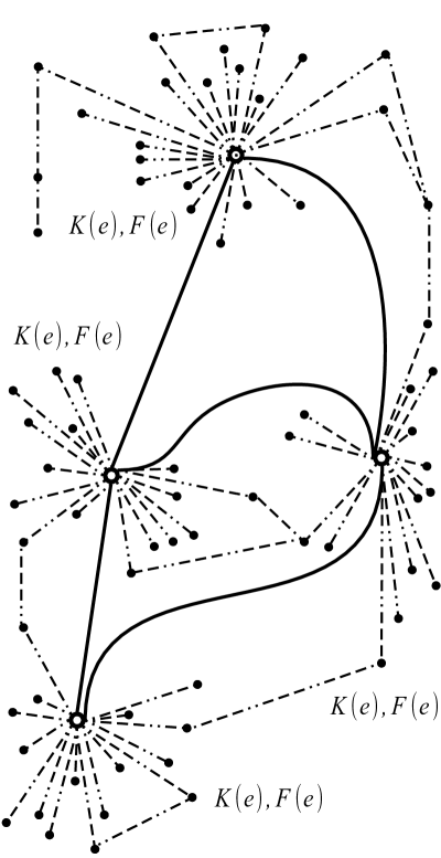
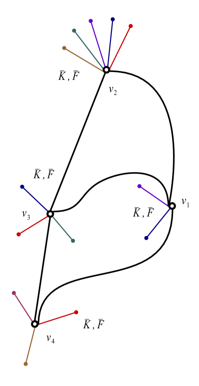
2 Preliminaries

2.1 Metric Graphs and Function Spaces

We begin this section recalling some facts for embeddings of graphs.

Definition 1

A graph $G=(V,E)$ is said to be embeddable in $\bm{\mathbbm{R}}^{\!N}$ if it can be drawn in $\bm{\mathbbm{R}}^{\!N}$ so that its edges intersect only at their ends. A graph is said to be planar if it can be embedded in the plane.

It is a well-known fact that any simple graph can be embedded in $\bm{\mathbbm{R}}^{\!2}$ or $\bm{\mathbbm{R}}^{\!3}$ (depending whether it is planar or not) in a way that its edges are drawn with straight lines; see [16] for planar graphs and [17] for non-planar graphs. In the following it will always be assumed that the graph is already embedded in $\bm{\mathbbm{R}}^{\!2}$ or $\bm{\mathbbm{R}}^{\!3}$.

Definition 2

Let $G=(V,E)$ be a graph embedded in $\bm{\mathbbm{R}}^{2}$ or $\bm{\mathbbm{R}}^{3}$, depending on the case.

1. The graph $G$ is said to be a metric graph if each edge $e\in E$ is assigned a positive length $\ell_{e}\in(0,\infty)$.

2. The graph $G$ is said to be locally finite if $\deg(v)<+\infty$ for all $v\in V$.

3. If the graph $G$ is metric, the boundary of the graph is defined by the set of vertices of degree one. The set will also be denominated as the set of boundary vertices and denoted by

   $$\partial V\overset{\mathbf{def}}{=}\{v\in V:\deg(v)=1\}.$$ (2)

4. Given a metric graph we define its natural domain by

   $$\Omega_{G}\overset{\mathbf{def}}{=}\bigcup_{e\,\in\,E}\operatorname*{int}(e).$$ (3)

Definition 3

Let $G=(V,E)$ be metric graph we define the following associated Hilbert spaces

1. The space of square integrable functions, or mass space is defined by

   $$L^{2}(G)\overset{\mathbf{def}}{=}\bigoplus_{e\,\in\,E}L^{2}(e),$$ (4a)

   endowed with its natural inner product

   $$\langle f,g\rangle_{L^{2}(G)}\overset{\mathbf{def}}{=}\sum_{e\,\in\,E}\int_{e}f\,g.$$ (4b)

2. The energy space of functions is defined by

   $$H^{1}(G)\overset{\mathbf{def}}{=}\Big{\{}f\in\bigoplus_{e\,\in\,E}H^{1}(e):\lim_{\begin{subarray}{c}x\,\rightarrow\,v\\ x\,\in\,e\end{subarray}}f(x)=\lim_{\begin{subarray}{c}x\,\rightarrow\,v\\ x\,\in\,\sigma\end{subarray}}f(x)\,,\\ \text{for all vertices}\,v\in V\,\text{and for all edges }\;e,\sigma\;\text{ incident on}\;v\Big{\}}.$$ (5a)

   In the sequel $$f(v)\overset{\mathbf{def}}{=}\lim\{f(x):x\,\rightarrow\,v,\,x\,\in\,e\} e\in E v$$, with any edge incident on . We endow the space with its natural inner product

   $$\langle f,g\rangle_{H^{1}(G)}\overset{\mathbf{def}}{=}\sum_{e\,\in\,E}\int_{e}f\,g+\sum_{e\,\in\,E}\int_{e}\bm{\partial}_{e}f\,\bm{\partial}_{e}g.$$ (5b)

   Here $\bm{\partial}_{e}$ denotes the derivative along the edge $e\in E$.

3. The space $H_{0}^{1}(G)$ is defined by

   $$H_{0}^{1}(G)\overset{\mathbf{def}}{=}\big{\{}f\in H^{1}(G):f(v)=0\,,\;\text{for all}\;v\in\partial V\big{\}},$$ (6)

   endowed with the standard inner product (5b).

Remark 1

Let $G$ be a metric graph

1. Notice that the definition of $\bm{\partial}_{e}$ is ambiguous in the expression (5b), such ambiguity will cause no problems since the bilinear structure of the inner product is indifferent to the choice of direction

   $$(q,r)\mapsto\bm{\partial}_{e}q\,\bm{\partial}_{e}r=\big{(}-\bm{\partial}_{e}q\big{)}\,(-\bm{\partial}_{e}r).$$

2. Whenever there is need to specify the direction of the derivate, we write $\bm{\partial}_{e,v}$ to indicate the direction pointing from the interior of the edge $e$ towards the vertex $v$ on one of its extremes.

3. Notice that if the metric graph $G$ is connected, then the Poincaré inequality holds and the inner product

   $$(f,g)\mapsto\sum_{e\,\in\,E}\int_{e}\bm{\partial}_{e}f\,\bm{\partial}_{e}g,$$ (7)

   is equivalent to the standard one (5b) in the space $H_{0}^{1}(G)$.

4. Observe that the condition of agreement of a function $f\in H^{1}(G)$ on the vertices of the graph $G$ does not necessarily imply continuity as a function $f:\Omega_{G}\rightarrow\bm{\mathbbm{R}}$. For if the degree of a vertex $v\in V$ is infinite and the function is continuous on $v$, then it follows that the convergence $f(v)\overset{\mathbf{def}}{=}\lim\{f(x):x\,\rightarrow\,v,\,x\,\in\,e\}$ is uniform for all the edges $e$ incident on $v$. Such a condition can not be derived from the norm induced by the inner product (5b), although the function $f\bm{\mathbbm{1}}_{\operatorname*{int}(e)}$ is continuous for all $e\in E$.

Definition 4

Let $G_{n}=(V_{n},E_{n})$ be a sequence of graphs.

1. The sequence $\{G_{n}:n\in\bm{\mathbbm{N}}\}$ is said to be increasing if $V_{n}\subseteq V_{n+1}$ and $E_{n}\subseteq E_{n+1}$ for all $n\in\bm{\mathbbm{N}}$.

2. Given an increasing sequence of graphs $\{G_{n}:n\in\bm{\mathbbm{N}}\}$, we define the limit graph $G=(V,E)$ in the natural way i.e.,

   $$V\overset{\mathbf{def}}{=}\bigcup_{n\,\in\,\bm{\mathbbm{N}}}V_{n} E\overset{\mathbf{def}}{=}\bigcup_{n\,\in\,\bm{\mathbbm{N}}}E_{n}.$$

   In analogy with monotone sequences of sets we adopt the notation

   $$G\overset{\mathbf{def}}{=}\bigcup_{n\,\in\,\bm{\mathbbm{N}}}G_{n}.$$ (8)

2.2 The Strong and Weak Forms of the Stationary Diffusion Problem on Graphs

Definition 5

Let $G=(V,E)$ be a locally finite metric graph, $F\in L^{2}(G)$ and $h:V-\bm{\partial}V\rightarrow\bm{\mathbbm{R}}$, define the following diffusion problem

$$\sum_{e\,\in\,E}-\bm{\partial}_{e}\big{(}K\bm{\partial}_{e}p\big{)}\bm{\mathbbm{1}}_{e}=\sum_{e\,\in\,E}F\,\bm{\mathbbm{1}}_{e}\quad\text{in}\;\Omega_{G}.$$ (9a)

Where $$K\in L^{\infty}(\Omega_{G})$$ is a nonnegative diffusion coefficient. We endow the problem with normal stress continuity conditions

$$\lim_{\begin{subarray}{c}x\,\rightarrow\,v\\ x\,\in\,e\end{subarray}}p(x)=p(v)\quad\text{for all }\;p\in V-\partial V,$$ (9b)

and normal flux balance conditions

$$h(v)+\sum_{\begin{subarray}{c}e\,\in\,E\\ e\,\text{incident on}\,v\end{subarray}}\lim_{\begin{subarray}{c}x\rightarrow v\\ x\,\in\,e\end{subarray}}\bm{\partial}_{e,v}\,p(x)=0\quad\text{for all }\;v\in V-\partial V.$$ (9c)

Here $$\bm{\partial}_{e,v} e v$$ denotes the derivative along the edge pointing away from the vertex . Finally, we declare homogeneous Dirichlet boundary conditions

$$p(v)=0\quad\text{for all }\;v\in\partial V.$$ (9d)

A weak variational formulation of this problem is given by

$$p\in H^{1}_{0}(G): \sum_{e\,\in\,E}\int_{e}K\bm{\partial}_{e}p\,\bm{\partial}_{e}q=\sum_{e\,\in\,E}\int_{e}F\,q+\sum_{v\,\in\,V-\partial V}h(v)\,q(v) \forall\,q\in H^{1}_{0}(G).$$ (10)

For the sake of completeness we present the following standard result.

Proposition 1

Let $G=(V,E)$ be a locally finite connected metric graph such that $\partial V\neq\emptyset$ and let $K\in L^{\infty}(\Omega_{G})$ be a diffusion coefficient such that $K(x)\geq c_{K}>0$ almost everywhere in $\Omega_{G}$. Then the problem (10) is well-posed.

Proof 1

Clearly the functionals on the right hand side of Problem (10) are linear and continuous, as well as the bilinear form $b(p,q)\overset{\mathbf{def}}{=}\sum_{e\,\in\,E}\int_{e}K\bm{\partial}_{e}p\,\bm{\partial}_{e}q$ of the left hand side. Additionally,

$$\sum_{e\,\in\,E}\int_{e}K|\bm{\partial}_{e}p|^{2}\geq c_{K}\sum_{e\,\in\,E}\int_{e}|\bm{\partial}_{e}p|^{2}\geq\tilde{c}\sum_{e\,\in\,E}\|p\|_{H^{1}(e)}^{2}=\tilde{c}\,\|p\|_{H^{1}(G)}^{2}.$$

The first inequality above holds due to the conditions on $K$. The second inequality hods due to the Dirichlet homogeneous boundary conditions and the connectedness of the graph $G$, which permits the Poincaré inequality on the space $H^{1}_{0}(G)$ as discussed in Remark 1 (iii) above. Therefore, due to the Lax-Milgram Theorem, the Problem (10) is well-posed.

2.3 Equidistributed Sequences and Weyl’s Theorem

The brief review of equidistributed sequences and Weyl’s theorem of this section will be applied, almost exclusively in the numerical examples below, see Section 5. For a complete exposition on equidistributed sequences and Weyl’s Theorem see [18].

Definition 6

A sequence $\{\theta_{n}:n\in\bm{\mathbbm{N}}\}$ is called equidistributed on an interval $[a,b]$ if for each subinterval $[c,d]\subseteq[a,b]$ it holds that:

$$\lim\limits_{n\to\infty}\frac{\#\{i:\theta_{i}\in[c,d],1\leq i\leq n\}}{n}=\frac{d-c}{b-a}.$$ (11)

Theorem 2 (Weyl’s Theorem)

Let $\big{\{}\theta_{n}:n\in\bm{\mathbbm{N}}\big{\}}$ be a sequence on $[a,b]$, the following conditions are equivalent:

1. The sequence $\{\theta_{n}:n\in\bm{\mathbbm{N}}\}$ is equidistributed in $[a,b]$.

2. For every Riemann integrable function $f:[a,b]\to\bm{\mathbbm{C}}$

   $$\lim\limits_{n\to\infty}\frac{1}{n}\sum\limits_{i=1}^{n}f(\theta_{i})=\frac{1}{b-a}\int_{a}^{b}f(\theta)\,d\theta.$$

Definition 7

Let $\Omega=B(0,1)\subseteq\bm{\mathbbm{R}}^{2}$ and let $f:\Omega\rightarrow\bm{\mathbbm{R}}$ be such that its restriction to every sphere $\partial B(0,\rho)$ with $0\leq\rho<1$ is Riemann integrable. Then, we define its angular average by the average value of $f$ along the sphere $\partial(B(0,\rho))$, i.e.,

$$\operatorname*{m_{\theta}}[f]:[0,1)\rightarrow\bm{\mathbbm{R}}\,, \operatorname*{m_{\theta}}[f](t)\overset{\mathbf{def}}{=}\frac{1}{2\pi}\int_{0}^{2\pi}f\big{(}t\cos\theta,\,t\sin\theta)\big{)}\,d\theta.$$ (12)

3 The Sequence of Problems

In this section we analyze the behavior of the solutions $\{p^{n}:n\in\bm{\mathbbm{N}}\}$ of a family of well-posed problems on an very particular increasing sequence of graphs $\{G_{n}:n\in\bm{\mathbbm{N}}\}$, depicted in Figure 2.

3.1 Geometric Setting and the n-Stage Problem

In the following we denote by $\Omega$, $S^{1}$ the unit disk and the unit sphere in $\bm{\mathbbm{R}}^{2}$ respectively. The function $F:\Omega_{G}\rightarrow\bm{\mathbbm{R}}$ is such that $F\bm{\mathbbm{1}}_{\Omega_{n}}\in L^{2}(\Omega_{n})$ for all $n\in\bm{\mathbbm{N}}$, $\{h^{n}:n\in\bm{\mathbbm{N}}\}$ is a sequence of real numbers and the diffusion coefficient $K\in L^{\infty}(\Omega_{G})$ is such that $K(\cdot)\geq c_{K}>0$ almost everywhere in $\Omega_{G}$.

Definition 8

Let $\{v_{n}:n\geq 1\}$ be an equidistributed sequence in $S^{1}$ and $v_{0}\overset{\mathbf{def}}{=}0\in\bm{\mathbbm{R}}^{2}$.

1. For each $n\in\bm{\mathbbm{N}}$ define the graph $G_{n}=(V_{n},E_{n})$ in the following way:

   $$V_{n}\overset{\mathbf{def}}{=}\{v_{n}:0\leq i\leq n\}, E_{n}\overset{\mathbf{def}}{=}\{v_{0}v_{i}:1\leq i\leq n\}.$$ (13)

2. For the increasing sequence of graphs $\{G_{n}:n\in\bm{\mathbbm{N}}\}$ define the limit graph $G\overset{\mathbf{def}}{=}\bigcup_{n\,\in\,\bm{\mathbbm{N}}}G_{n}$ as described in Definition 4.

3. In the following we denote the natural domains corresponding to $G$, $G_{n}$ by $\Omega_{G}$ and $\Omega_{n}$ respectively.

4. For any edge $e\in E$ we denote by $v_{e}$ its boundary vertex and $\theta_{e}\in[0,2\pi]$ the direction of the edge.

5. From now on, for each edge $e=v_{0}v_{e}$ and $f:e\rightarrow\bm{\mathbbm{R}}$ a function, it will be understood that its one-dimensional parametrization, is oriented from the central vertex $v_{0}$ to the boundary vertex $v_{e}$. Consequently the derivative $\bm{\partial}_{e}$ equals $\bm{\partial}_{e,v_{e}}$.

6. For any given function $f:\Omega_{G}\rightarrow\bm{\mathbbm{R}}$ (or $f:\Omega_{n}\rightarrow\bm{\mathbbm{R}}$) we denote by $f_{e}:(0,1)\rightarrow\bm{\mathbbm{R}}$, the real variable function $f_{e}(t)\overset{\mathbf{def}}{=}(f\bm{\mathbbm{1}}_{e})(t\cos\theta_{e},t\sin\theta_{e})$ on the edges $e\in E$ (or $e\in E_{n}$ respectively).

   

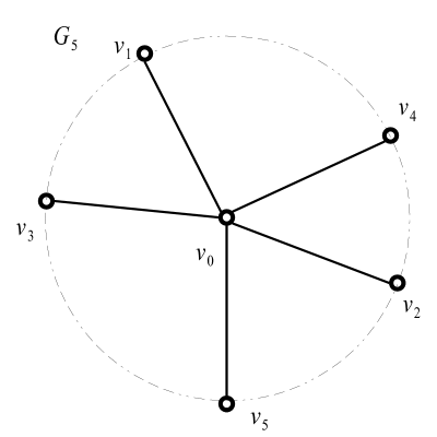
   (a) Graph Stage 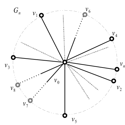$5$.

   

   (b) Graph Stage n.

   Figure 2: Figure (a) depicts the stage $5$ of the graph $G$. Figure (b) depicts a more general stage $n$ of the graph $G$.

Remark 2

From the following analysis, it will be clear that it is not necessary to assume that the sequence of vertices $\{v_{n}:n\in\bm{\mathbbm{N}}\}$ of the graph is equidistributed or that the vertices are in $S^{1}$ or even that the graph is embedded in $\bm{\mathbbm{R}}^{2}$. We adopt these assumptions, mainly to facilitate a geometric visualization of the setting.

From now on it will be assumed that $\{G_{n}:n\in\bm{\mathbbm{N}}\}$ is the increasing sequence of graphs, with $G$ its limit graph, as in the Definition 8 above. Next, we define the family of problems to be studied, for each $n\in\bm{\mathbbm{N}}$ consider the well-posed problem

$$p^{n}\in H^{1}_{0}(G_{n}): \sum_{e\,\in\,E_{n}}\int_{e}K\bm{\partial}_{e}p^{n}\,\bm{\partial}_{e}q=\sum_{e\,\in\,E_{n}}\int_{e}F\,q+h^{n}\,q(v_{0})\,, \forall\,q\in H^{1}_{0}(G_{n}).$$ (14)

We are to analyze the asymptotic behavior of the sequence of solutions $\{p^{n}:n\in\bm{\mathbbm{N}}\}$. One of the main challenges is that the elements of the sequence are not defined on the same global space. The fact that $p^{n}(0)$ may not be zero makes impossible to extend this function to $H_{0}^{1}(G)$ directly, however it will play a central role in the asymptotic analysis of the problem.

3.2 Estimates and Edgewise Convergence Statements

In this section we get estimates for the sequence of solutions, several steps have to be made as it is not direct to attain them. We start introducing conditions to be assumed from now on

Hypothesis 1

1. The forcing term $F$ is defined in the whole domain, i.e. $F:\Omega_{G}\rightarrow\bm{\mathbbm{R}}$ and $M\overset{\mathbf{def}}{=}\sup_{e\,\in\,E}\|F\|_{L^{2}(e)}<+\infty$.

2. The sequence $\big{\{}\dfrac{1}{n}\,h^{n}:n\in\bm{\mathbbm{N}}\big{\}}$ is bounded.

3. The permeability coefficient satisfies that $K\in L^{\infty}(\Omega_{G})$, $\inf_{x\,\in\,\Omega_{G}}K(x)=c_{K}>0$ and $K\bm{\mathbbm{1}}_{e}=K(e)$ i.e., it is constant along each edge $e\in E$.

Remark 3

Notice that the Hypothesis 1-(ii) states that the balance of normal flux on the central vertex is of order $O(n)$ i.e., it scales with the number of incident edges.

Lemma 3

Under the Hypothesis 1, the following facts hold

1. The sequence $\{p^{n}(0):n\in\bm{\mathbbm{N}}\}\subseteq\bm{\mathbbm{R}}$ is bounded.

2. Let $e\in E$ be an edge of the graph $G$ then, the sequence $\{\bm{\partial}_{e}p^{n}(0):e\in E_{n}\}\subseteq\bm{\mathbbm{R}}$ is bounded. Moreover, there exists $M_{0}$ such that $|\bm{\partial}_{e}p^{n}(0)|\leq M_{0}$ for all $e\in E$ and $n\in\bm{\mathbbm{N}}$ such that $e\in E_{n}$.

3. Suppose that the sequences $\big{\{}\dfrac{1}{n}\sum_{e\in E_{n}}\int_{0}^{1}(t-1)F_{e}(t)dt:n\in\bm{\mathbbm{N}}\big{\}}$, $\big{\{}\dfrac{1}{n}\,h^{n}:n\in\bm{\mathbbm{N}}\big{\}}$ and $\big{\{}\dfrac{1}{n}\sum_{e\in E_{n}}K(e):n\in\bm{\mathbbm{N}}\big{\}}$ are convergent, then the following limits are satisfied

   $$\lim_{n\rightarrow\infty}p^{n}(0)=\lim_{n\rightarrow\infty}\frac{\frac{1}{n}\sum_{e\in E_{n}}\int_{0}^{1}(t-1)F_{e}(t)dt-\frac{1}{n}h^{n}}{\frac{1}{n}\sum_{e\in E_{n}}K(e)}.$$ (15a)

   For any fixed edge $$e\in E$$ holds

   $$\lim_{n\rightarrow\infty}K(e)\bm{\partial}_{e}p^{n}(0)=L(e)\overset{\mathbf{def}}{=}\int_{0}^{1}(t-1)F_{e}(t)dt-K(e)\lim_{n\rightarrow\infty}\frac{\frac{1}{n}\sum_{\sigma\in E_{n}}\int_{0}^{1}(t-1)F_{\sigma}(t)dt-\frac{1}{n}h^{n}}{\frac{1}{n}\sum_{\sigma\in E_{n}}K(\sigma)}\,.$$ (15b)

   Moreover, the convergence is uniform in the following sense

   $$\forall\,\epsilon>0\,\;\exists\,N\in\bm{\mathbbm{N}}\;\text{such that, if}\;n>N\,\text{and }\,e\in E_{n},\;\text{then }\;|K(e)\,\bm{\partial}_{e}p^{n}(0)-L(e)|<\epsilon\,.$$ (15c)

Proof 2

1. Let $q\in H_{0}^{1}(G_{n})$ be the function such that $q(0)=-1$ and $q_{e}(t)=t-1$ for all $e\in E_{n}$. Test (14) with $q$, this yields

   $$q(0)\sum_{e\,\in\,E_{n}}K\int_{e}\bm{\partial}_{e}p^{n}=\sum_{e\,\in\,E_{n}}\int_{e}Fq+h^{n}\,q(0).$$ (16)

   Computing and doing some estimates we get

   $$\#E_{n}\,c_{K}\,|p^{n}(0)|\leq\frac{1}{\sqrt{3}}\sum_{e\,\in\,E_{n}}\|F\|_{L^{2}(e)}+|h^{n}|.$$

   Hence

   $$|p^{n}(0)|\leq\frac{1}{c_{K}}M+\frac{1}{c_{K}}\,\Big{|}\frac{h^{n}}{n}\Big{|}.$$

   This proves the first part.

2. Let $e\in E$ be a fixed edge, let $n\in\bm{\mathbbm{N}}$ be such that $e\in E_{n}$ and let $p^{n}$ be the solution to Problem (14). Let $q\in H_{0}^{1}(G_{n})$ be as in the previous part and test (14) to get

   $$\begin{split}-K(e)p^{n}(0)\,q(0)+\sum_{\begin{subarray}{c}\sigma\,\in\,E_{n}\\ \sigma\neq e\end{subarray}}K\int_{\sigma}\bm{\partial}_{\sigma}p^{n}\,\bm{\partial}_{\sigma}q&=K(e)\,p^{n}(0)-\sum_{\begin{subarray}{c}\sigma\,\in\,E_{n}\\ \sigma\neq e\end{subarray}}K\int_{\sigma}\bm{\partial}_{\sigma}^{2}p^{n}\,q+q(0)\sum_{\begin{subarray}{c}\sigma\,\in\,E_{n}\\ \sigma\neq e\end{subarray}}K\,\bm{\partial}_{\sigma}p^{n}(0)\,\\ &=\int_{e}Fq+\sum_{\begin{subarray}{c}\sigma\,\in\,E_{n}\\ \sigma\neq e\end{subarray}}\int_{\sigma}Fq+h^{n}\,q(0).\end{split}$$

   In the expression above, integration by parts was applied to each summand $\sigma\neq e$ of the left hand side, in order to get the second equality. Now, recalling that $\sum_{e\,\in E_{n}}K\,\bm{\partial}_{e}p^{n}(0)=h^{n}$ and that $-K\bm{\mathbbm{1}}_{e}\bm{\partial}_{e}^{2}p^{n}=F\bm{\mathbbm{1}}_{e}$ for each $e\in E_{n}$ the equality above reduces to

   $$K(e)p^{n}(0)=\int_{0}^{1}(t-1)F_{e}(t)dt-K(e)\bm{\partial}_{e}\,p^{n}(0).$$ (17)

   Hence,

   $$|\bm{\partial}_{e}\,p^{n}(0)|\leq|p^{n}(0)|+\frac{1}{c_{K}}\,\|F\|_{L^{2}(e)}\leq\frac{2}{c_{K}}M+\frac{1}{c_{K}}\,\Big{|}\frac{h^{n}}{n}\Big{|}.$$ (18)

   Choosing $M_{0}>0$ large enough, the result follows.

3. Let $q\in H_{0}^{1}(G_{n})$ be as in the previous part, testing (14) with it yields the equality (16) which is equivalent to

   $$p^{n}(0)\,\frac{1}{n}\sum_{e\,\in\,E_{n}}K=\frac{1}{n}\sum_{e\,\in\,E_{n}}\int_{e}Fq+\frac{1}{n}\,h^{n}\,q(0).$$

   Now, letting $n\rightarrow\infty$ the equality (15a) follows because the hypothesis $K(e)>c_{K}$ for all $e\in E$ implies that $\dfrac{1}{n}\sum_{e\,\in\,E_{n}}K(e)\geq c_{K}>0$. For the convergence of $\{\bm{\partial}_{e}p^{n}(0):e\in E_{n}\}$, let $n\rightarrow\infty$ in the expression (17) to get the equality (15b). For the uniform convergence observe that the identity (17) yields

   $$\begin{split}\big{|}K(e)\bm{\partial}_{e}p^{n}(0)-L(e)\big{|}&=\Big{|}K(e)\lim_{n\rightarrow\infty}\frac{\frac{1}{n}\sum_{\sigma\in E_{n}}\int_{0}^{1}(t-1)F_{\sigma}(t)dt-\frac{1}{n}h^{n}}{\frac{1}{n}\sum_{\sigma\in E_{n}}K(\sigma)}-K(e)p^{n}(0)\Big{|}\\ &\leq\|K\|_{L^{\infty}}\Big{|}\lim_{n\rightarrow\infty}\frac{\frac{1}{n}\sum_{\sigma\in E_{n}}\int_{0}^{1}(t-1)F_{\sigma}(t)dt-\frac{1}{n}h^{n}}{\frac{1}{n}\sum_{\sigma\in E_{n}}K(\sigma)}-p^{n}(0)\Big{|}.\end{split}$$

   Finally, choose $N\in\bm{\mathbbm{N}}$ such that the right hand side of the expression above is less than $\epsilon>0$ for all $n>N$ then, the term of the left hand side is also dominated by $\epsilon>0$ for all $n>N$ and $e\in E_{n}$.

Remark 4

It is clear that in Lemma 3 part (iii), it suffices to require the mere existence of the limit

$$\lim_{n\rightarrow\infty}\frac{\sum_{\sigma\in E_{n}}\int_{0}^{1}(t-1)F_{\sigma}(t)dt-h^{n}}{\sum_{\sigma\in E_{n}}K(\sigma)}\,,$$

in order to attain the same conclusion. However, the hypotheses of (iii) are necessary to identify the asymptotic problem and compute the effective coefficients.

Theorem 4

Let $F$, $\{h^{n}:n\in\bm{\mathbbm{N}}\}$ and $K$ verify the Hypothesis 1 as in Lemma 3 then

1. There exists a constant $M_{1}$ such that $\|p^{n}\|_{H^{2}(e)}\leq M_{1}$ for all $e\in E$ and $n\in\bm{\mathbbm{N}}$ such that $e\in E_{n}$.

2. For each $e\in E$ there exists $p^{(e)}\in H^{1}(e)$ such that $\|p^{n}\bm{\mathbbm{1}}_{e}-p^{(e)}\|_{H^{1}(e)}\xrightarrow[n\,\rightarrow\,\infty]{}0$. Moreover, this convergence is uniform in the following sense

   $$\forall\,\epsilon>0\,\;\exists\,N\in\bm{\mathbbm{N}}\;\text{such that, if}\;n>N\,\text{and }\,e\in E_{n},\;\text{then }\;\|\bm{\partial}_{e}p^{n}-\bm{\partial}_{e}p^{(e)}\|_{H^{1}(e)}<\epsilon\,.$$ (19)

3. The function $p:\Omega_{G}\rightarrow\bm{\mathbbm{R}}$ given by $p\bm{\mathbbm{1}}_{e}\overset{\mathbf{def}}{=}p^{(e)}$ is well-defined and it will be referred to as the limit function.

Proof 3

1. Fix $e\in E$ and let $n\in\bm{\mathbbm{N}}$ be such that $e\in E_{n}$. Since $p^{n}$ is the solution of Problem (14) it follows that $-K(e)\,\bm{\partial}_{e}^{2}p^{n}=F\bm{\mathbbm{1}}_{e}\in L^{2}(e)$ for all $e\in E_{n}$, in particular $p^{n}\bm{\mathbbm{1}}_{e}\in H^{2}(e)$ with $\|\bm{\partial}_{e}^{2}p^{n}\|_{L^{2}(e)}\leq\dfrac{1}{c_{K}}\,\|F\|_{L^{2}(e)}\leq\dfrac{1}{c_{K}}M$. On the other hand, since $\bm{\partial}_{e}p^{n}\,\bm{\mathbbm{1}}_{e}$ is absolutely continuous, the fundamental theorem of calculus applies, hence $\bm{\partial}_{e}p^{n}(x)=\bm{\partial}_{e}p^{n}(0)+\int_{0}^{x}\bm{\partial}^{2}p^{n}_{e}(t)\,dt=\bm{\partial}_{e}p^{n}(0)+\int_{0}^{x}F_{e}(t)\,dt$ for all $x\in e$. Therefore,

   $$|\bm{\partial}_{e}p^{n}(x)|^{2}=2|\bm{\partial}_{e}p^{n}(0)|^{2}+2\,x\,\|F\|_{L^{2}(e)}^{2}\leq 2\,M_{0}^{2}+2M^{2}.$$

   Where $M_{0}$ is the global bound found in Lemma 3-(ii) above. Integrating along the edge $e$ gives $\|\bm{\partial}_{e}p^{n}\|_{L^{2}(e)}\leq\sqrt{2(M_{0}^{2}+M^{2})}$. Next, given that $p^{n}(v)=0$ for all $v\in E_{n}$, repeating the previous argument yields $\|p^{n}\|_{L^{2}(e)}\leq\sqrt{2(M_{0}^{2}+M^{2})}$. Finally, since $\|\bm{\partial}_{e}^{2}p^{n}\|_{L^{2}}(e)\leq\dfrac{1}{c_{K}}M$, the result follows for any $M_{1}$ satisfying

   $$M_{1}^{2}\geq 4M_{0}^{2}+\Big{(}4+\frac{1}{c_{K}^{2}}\Big{)}M^{2}.$$

2. Fix $e\in E$, due to the previous part the sequence $\{p^{n}\bm{\mathbbm{1}}_{e}:e\in E_{n}\}$ is bounded in $H^{2}(e)$, then there exists $p^{(e)}\in H^{2}(e)$ and a subsequence $\{n_{k}:k\in\bm{\mathbbm{N}}\}$ such that

   $$p^{n_{k}}\xrightarrow[k\,\rightarrow\,\infty]{}p^{(e)}\quad\text{weakly in}\,H^{2}(e)\;\text{and strongly in}\,H^{1}(e).$$

   Let $\varphi\in H^{1}(e)$ such that equals zero on the boundary vertex of $e$. Let $q$ be the function in $H_{0}^{1}(G_{n})$ such that $q_{e}=\varphi$ and $q_{\sigma}(t)=\varphi(0)(1-t)$ is linear for all $\sigma\in E_{n}-\{e\}$. Test Problem (14) with this function to get

   $$\int_{e}K(e)\bm{\partial}_{e}p^{n}\,\bm{\partial}_{e}q+\sum_{\begin{subarray}{c}\sigma\,\in\,E_{n}\\ \sigma\neq e\end{subarray}}K\int_{\sigma}\bm{\partial}_{\sigma}p^{n}\,\bm{\partial}_{\sigma}q=\int_{e}Fq+\sum_{\begin{subarray}{c}\sigma\,\in\,E_{n}\\ \sigma\neq e\end{subarray}}\int_{\sigma}Fq+h^{n}\,q(0).$$

   Integrating by parts the second summand of the left hand side yields

   $$\int_{e}K(e)\bm{\partial}_{e}p^{n}\,\bm{\partial}_{e}\varphi-\sum_{\begin{subarray}{c}\sigma\,\in\,E_{n}\\ \sigma\neq e\end{subarray}}K\int_{\sigma}\bm{\partial}_{\sigma}^{2}p^{n}\,q-\varphi(0)\sum_{\begin{subarray}{c}\sigma\,\in\,E_{n}\\ \sigma\neq e\end{subarray}}K\,\bm{\partial}_{\sigma}p^{n}(0)=\int_{e}F\varphi+\sum_{\begin{subarray}{c}\sigma\,\in\,E_{n}\\ \sigma\neq e\end{subarray}}\int_{\sigma}F\varphi+h^{n}\,q(0).$$

   Since $p^{n}$ is a solution of the problem, the above reduces to

   $$\int_{e}K(e)\bm{\partial}_{e}p^{n}\,\bm{\partial}_{e}\varphi+K(e)\bm{\partial}_{e}p^{n}(0)\,\varphi(0)=\int_{e}Fq.$$ (20)

   Equality (20) holds for all $n\in\bm{\mathbbm{N}}$, in particular it holds for the convergent subsequence $\{n_{k}:k\in\bm{\mathbbm{N}}\}$, taking limit on this sequence and recalling (15b), we have

   $$\int_{e}K(e)\bm{\partial}_{e}p^{(e)}\,\bm{\partial}_{e}\varphi=\int_{e}F\varphi-L(e)\,\varphi(0).$$ (21)

   The statement (21) holds for all $\varphi\in H^{1}(e)$ vanishing at $v_{e}$, the boundary vertex of $e$. Define the space $H(e)\overset{\mathbf{def}}{=}\{\varphi\in H^{1}(e):\varphi(v_{e})=0\}$ and consider the problem

   $$u\in H(e): \int_{e}K(e)\bm{\partial}_{e}u\,\bm{\partial}_{e}\varphi=\int_{e}F\varphi-L(e)\,\varphi(0)\,, \forall\,\varphi\in H(e).$$ (22)

   Due to the Lax-Milgram Theorem the problem above is well-posed, additionally it is clear that $p^{(e)}\in H(e)$, therefore it is the unique solution to the Problem (22) above. Now, recall that $\{p^{n}\bm{\mathbbm{1}}_{e}:e\in E_{n}\}$ is bounded in $H^{2}(e)$ and that the previous reasoning applies for every strongly $H^{1}(e)$-convergent subsequence, therefore its limit is the unique solution to Problem (22). Consequently, due to Rellich-Kondrachov, it follows that the whole sequence converges strongly. Next, for the uniform convergence test both statements (20) and (21) with $(p^{n}\bm{\mathbbm{1}}_{e}-p^{(e)})$ and subtract them to get

   $$\begin{split}c_{K}\|\bm{\partial}_{e}p^{n}-\bm{\partial}_{e}p^{(e)}\|^{2}_{H^{1}(e)}\leq K(e)\int_{e}\big{|}\bm{\partial}_{e}p^{n}-\bm{\partial}_{e}p^{(e)}\big{|}^{2}&=\big{(}L(e)-K(e)\bm{\partial}_{e}p^{n}(0)\big{)}\big{(}p^{n}(0)-p^{(e)}(0)\big{)}\\ &\leq\big{|}L(e)-K(e)\bm{\partial}_{e}p^{n}(0)\big{|}\,\|\bm{\partial}_{e}p^{n}-\bm{\partial}_{e}p^{(e)}\|_{H^{1}(e)}.\end{split}$$

   The above yields

   $$\|\bm{\partial}_{e}p^{n}-\bm{\partial}_{e}p^{(e)}\|_{H^{1}(e)}\leq\frac{1}{c_{K}}\,\big{|}L(e)-K(e)\bm{\partial}_{e}p^{n}(0)\big{|}.$$

   Now, the uniform convergence (19) follows from the Statement (15c), which concludes the second part.

3. Since $p^{(e)}(0)=\lim\limits_{n\to\infty}p^{n}(0)$ for all $e\in E$ then, the limit function $p$ is well-defined and the proof is complete.

4 The Homogenized Problem: a Cesàro Average Approach

In this section we study the asymptotic properties of the global behavior of the solutions $\{p^{n}:n\in\bm{\mathbbm{N}}\}$. It will be seen that such analysis must be done for certain type of “Cesàro averages” of the solutions. This is observed by the techniques and the hypotheses of Lemma 3, which are necessary to conclude the local convergence of $\{p^{n}\bm{\mathbbm{1}}_{e}:e\in E_{n}\}$. Additionally, the type of estimates and the numerical experiments suggest this physical magnitude as the most significant for global behavior analysis and upscaling purposes. We start introducing some necessary hypotheses.

Hypothesis 2

Suppose that $F$, $\{h^{n}:n\in\bm{\mathbbm{N}}\}$ and $K$ verify Hypothesis 1 and, additionally

1. The diffusion coefficient $K:\Omega_{G}\rightarrow(0,\infty)$ has finite range. Moreover, if $K(E)=\{K_{i}:1\leq i\leq I\}$ and $B_{i}\overset{\mathbf{def}}{=}\{e\in E:K(e)=K_{i}\}$, then

   $$\frac{1}{n}\sum_{e\,\in\,E_{n}\cap B_{i}}K(e)=\frac{\#(E_{n}\cap B_{i})}{n}K_{i}\xrightarrow[n\,\rightarrow\,\infty]{}s_{i}\,K_{i}.$$ (23)

   With $s_{i}>0$ for all $1\leq i\leq I$ and such that $\sum\limits_{i=1}^{I}s_{i}=1$.

2. The forcing term $F$ satisfies that

   $$\frac{1}{\#(E_{n}\cap B_{i})}\sum_{e\,\in\,E_{n}\cap B_{i}}F_{e}\xrightarrow[n\,\rightarrow\,\infty]{}\accentset{\rule{2.79996pt}{0.5pt}}{F}_{i}\,, \forall\;1\leq i\leq I.$$ (24)

   Where $\accentset{\rule{2.79996pt}{0.5pt}}{F}_{i}\in L^{2}(0,1)$ and the sense of convergence is pointwise almost everywhere.

3. The sequence $\big{\{}\dfrac{1}{n}\,h^{n}:n\in\bm{\mathbbm{N}}\big{\}}$ is convergent with $\accentset{\rule{2.79996pt}{0.5pt}}{h}=\lim\limits_{n\rightarrow\infty}\dfrac{1}{n}\,h^{n}$.

Remark 5

1. Notice that if (i) and (ii) in Hypothesis 2 are satisfied, then

   $$\frac{1}{n}\sum_{e\,\in\,E_{n}}F_{e}=\sum_{i\,=\,1}^{I}\frac{\#(E_{n}\cap B_{i})}{n}\frac{1}{\#(E_{n}\cap B_{i})}\sum_{e\,\in\,E_{n}\cap B_{i}}F_{e}\xrightarrow[n\,\rightarrow\,\infty]{}\sum_{i\,=\,1}^{I}s_{i}\accentset{\rule{2.79996pt}{0.5pt}}{F}_{i}\,.$$

   Hence, the sequence $\{F_{e}:e\in E\}$ is Cesàro convergent.

2. A familiar context for the required convergence statement (24) in Hypothesis 2 above is the following. Let $F$ be a continuous and bounded function defined on the whole disk $\Omega$ and suppose that for each $1\leq i\leq I$, the sequence of vertices $\{v_{n}:n\in\bm{\mathbbm{N}},\,v_{n}v_{0}\in B_{i}\}$ is equidistributed on $S^{1}$. Then, due to Weyl’s Theorem 2, for any fixed $t\in(0,1)$ it holds that $\dfrac{1}{\#(E_{n}\cap B_{i})}\sum_{e\,\in\,E_{n}\cap B_{i}}F_{e}(t)\xrightarrow[n\,\rightarrow\,\infty]{}\operatorname*{m_{\theta}}[f]$ i.e, the angular average introduced in Definition 7.

4.1 Estimates and Cesàro Convergence Statements

Lemma 5

Let $F$, $\{h^{n}:n\in\bm{\mathbbm{N}}\}$ and $K$ verify Hypothesis 2 then

1. The sequence $\big{\{}\dfrac{1}{n}\sum_{e\,\in\,E_{n}}p^{n}_{e}:n\in\bm{\mathbbm{N}}\big{\}}$ is bounded in $H^{2}(0,1)$.

2. The sequence

   $$\Big{\{}\frac{1}{\#(E_{n}\cap B_{i})}\sum_{e\,\in\,E_{n}\cap B_{i}}p^{n}_{e}:n\in\bm{\mathbbm{N}}\Big{\}}$$ (25)

   is bounded in $H^{2}(0,1)$ for all $i\in\{1,\ldots,I\}$.

Proof 4

1. Test Problem (14) with $p^{n}$ to get

   $$\begin{split}c_{K}\sum_{e\,\in\,E_{n}}\|\bm{\partial}_{e}p^{n}\|_{L^{2}(e)}^{2}\leq\sum_{e\,\in\,E_{n}}\int_{e}K|\bm{\partial}p^{n}|^{2}&=\sum_{e\,\in\,E_{n}}\int_{e}F_{e}\,p^{n}+h^{n}\,p^{n}(v_{0})\\ &\leq\Big{(}\sum_{e\,\in\,E_{n}}\|F\|_{L^{2}(e)}^{2}\Big{)}^{1/2}\Big{(}\sum_{e\,\in\,E_{n}}\|p^{n}\|_{L^{2}(e)}^{2}\Big{)}^{1/2}+|h^{n}|\,|p^{n}(v_{0})|.\end{split}$$

   Since $p^{n}(v_{e})=0$ for all $e\in E_{n}$, then $\|p^{n}\|_{L^{2}(e)}\leq\|\bm{\partial}p^{n}\|_{L^{2}(e)}$ and $\|p^{n}\|_{H^{1}(e)}\leq\sqrt{2}\,\|\bm{\partial}p^{n}\|_{L^{2}(e)}$. Hence, dividing the above expression over $n$ gives

   $$\begin{split}\frac{1}{n}\sum_{e\,\in\,E_{n}}\|p^{n}\|_{H^{1}(e)}^{2}&\leq 2\,\Big{(}\frac{1}{n}\sum_{e\,\in\,E_{n}}\|F\|_{L^{2}(e)}^{2}\Big{)}^{1/2}\Big{(}\frac{1}{n}\sum_{e\,\in\,E_{n}}\|p^{n}\|_{H^{1}(e)}^{2}\Big{)}^{1/2}+2\,\frac{|h^{n}|}{n}\,|p^{n}(v_{0})|\\ &\leq 2\,\frac{M}{c_{K}}\Big{(}\frac{1}{n}\sum_{e\,\in\,E_{n}}\|p^{n}\|_{H^{1}(e)}^{2}\Big{)}^{1/2}+C\,.\end{split}$$

   Here $C>0$ is a generic constant independent from $n\in\bm{\mathbbm{N}}$. In the second line of the expression above, we used that $M=\sup_{e\in E_{n}}\|F\|_{L^{2}(e)}<+\infty$, $\{\frac{1}{n}\,h^{n}:n\in\bm{\mathbbm{N}}\}$ are bounded and that $\{p^{n}(v_{0}):n\in\bm{\mathbbm{N}}\}$ is convergent (therefore bounded) as stated in Lemma 3-(i). Hence, the sequence $x_{n}\overset{\mathbf{def}}{=}(\frac{1}{n}\sum_{e\,\in\,E_{n}}\|p^{n}\|_{H^{1}(e)}^{2})^{1/2}$ is such that $x_{n}^{2}\leq 2\,\frac{M}{c_{K}}\,x_{n}+C$ for all $n\in\bm{\mathbbm{N}}$, where the constants are all non-negative. Then $\{x_{n}:n\in\bm{\mathbbm{N}}\}$ must be bounded, but this implies

   $$\Big{\|}\frac{1}{n}\sum_{e\,\in\,E_{n}}p^{n}_{e}\Big{\|}_{H^{1}(0,1)}\leq\frac{1}{n}\sum_{e\,\in\,E_{n}}\|p^{n}_{e}\|_{H^{1}(0,1)}=\frac{1}{n}\sum_{e\,\in\,E_{n}}\|p^{n}\|_{H^{1}(e)}\leq\Big{(}\frac{1}{n}\sum_{e\,\in\,E_{n}}\|p^{n}\|_{H^{1}(e)}^{2}\Big{)}^{1/2}\,.$$

   Finally, recalling the estimate

   $$c_{K}\Big{\|}\frac{1}{n}\sum_{e\,\in\,E_{n}}\bm{\partial}^{2}p^{n}_{e}\Big{\|}_{L^{2}(0,1)}\leq\frac{1}{n}\sum_{e\,\in\,E_{n}}\big{\|}\bm{\partial}K(e)\bm{\partial}p^{n}_{e}\big{\|}_{L^{2}(0,1)}=\frac{1}{n}\sum_{e\,\in\,E_{n}}\|F\|_{L^{2}(0,1)}\leq M,$$

   the result follows.

2. Fix $i\in\{1,2,\ldots,I\}$ then

   $$\Big{\|}\frac{1}{\#(E_{n}\cap B_{i})}\sum_{e\,\in\,E_{n}\cap B_{i}}p^{n}_{e}\Big{\|}_{H^{2}(0,1)}\leq\frac{n}{\#(E_{n}\cap B_{i})}\,\frac{1}{n}\sum_{e\,\in\,E_{n}}\big{\|}p^{n}_{e}\big{\|}_{H^{2}(0,1)}.$$

   On the right hand side term of the expression above, the first factor is bounded due toHypothesis 2- (iii), while the boundedness of the second factor was shown in the previous part. Therefore, the result follows.

Before presenting the limit problem we introduce some necessary definitions and notation

Definition 9

Let $K$ verify Hypothesis 2 and $I=\#K(E)$ then

1. For all $1\leq i\leq I$ define $w_{i}\overset{\mathbf{def}}{=}\big{(}\cos(\frac{2\pi}{I}\,i),\sin(\frac{2\pi}{I}\,i)\big{)}\in S^{1}$, $w_{0}\overset{\mathbf{def}}{=}v_{0}=0$ and $\mathcal{V}\overset{\mathbf{def}}{=}\{w_{i}:0\leq i\leq I\}$.

2. For all $1\leq i\leq I$ define the edges $\sigma_{i}\overset{\mathbf{def}}{=}w_{0}w_{i}$ and ${\mathcal{E}}\overset{\mathbf{def}}{=}\{\sigma_{i}:1\leq i\leq I\}$.

3. Define the upscaled graph by ${\mathcal{G}}\overset{\mathbf{def}}{=}(\mathcal{V},{\mathcal{E}})$.

4. For any $\varphi\in H_{0}^{1}({\mathcal{G}})$ and $n\in\bm{\mathbbm{N}}$ denote by $T_{n}\varphi\in H_{0}^{1}(G_{n})$, the function such that $\big{(}T_{n}\varphi\big{)}\bm{\mathbbm{1}}_{e}$ agrees with $\varphi\bm{\mathbbm{1}}_{\sigma_{i}}$ whenever $e\in B_{i}$. This is summarized in the expression

   $$T_{n}\varphi=\sum_{e\,\in\,E_{n}}\big{(}T_{n}\varphi\big{)}\bm{\mathbbm{1}}_{e}\overset{\mathbf{def}}{=}\sum_{i\,=\,1}^{I}\;\sum_{e\,\in\,E_{n}\cap B_{i}}\big{(}\varphi\bm{\mathbbm{1}}_{\sigma_{i}}\big{)}\,.$$

   In the sequel we refer to $T_{n}\varphi$ as the $\bm{H_{0}^{1}(G_{n})}$-embedding of $\varphi$.

5. In the following, for any $1\leq i\leq I$, we adopt the notation $\bm{\partial}_{i}\overset{\mathbf{def}}{=}\bm{\partial}_{\sigma_{i}}$. Similarly, for any given function $f:\Omega_{{\mathcal{G}}}\rightarrow\bm{\mathbbm{R}}$ and edge $\sigma_{i}\in{\mathcal{E}}$ we denote by $f_{i}:(0,1)\rightarrow\bm{\mathbbm{R}}$, the real variable function $f_{i}(t)\overset{\mathbf{def}}{=}(f\bm{\mathbbm{1}}_{\sigma_{i}})\big{(}t\cos(\frac{2\pi}{I}i),t\sin(\frac{2\pi}{I}i)\big{)}$.

Theorem 6

Let $F$, $\{h^{n}:n\in\bm{\mathbbm{N}}\}$ and $K$ verify Hypothesis 2 then

1. The following problem is well-posed.

   $$\accentset{\rule{2.79996pt}{0.5pt}}{p}\in H_{0}^{1}({\mathcal{G}}): \sum_{i\,=\,1}^{I}\int_{\sigma_{i}}s_{i}K_{i}\,\bm{\partial}_{i}\accentset{\rule{2.79996pt}{0.5pt}}{p}\;\bm{\partial}_{i}q=\sum_{i\,=\,1}^{I}\int_{0}^{1}s_{i}\,\accentset{\rule{2.79996pt}{0.5pt}}{F}_{i}\,q_{i}+\accentset{\rule{2.79996pt}{0.5pt}}{h}(0)\,q(0)\,, \forall\,q\in H_{0}^{1}({\mathcal{G}}).$$ (26)

   In the sequel, we refer to Problem (26) as the upscaled or the homogenized problem and its solution $\accentset{\rule{2.79996pt}{0.5pt}}{p}$ as the upscaled or the homogenized solution indistinctly.

2. The sequence of solutions $\{p^{n}:n\in\bm{\mathbbm{N}}\}$ satisfy

   $$\Big{\|}\frac{1}{\#(E_{n}\cap B_{i})}\sum_{e\,\in\,E_{n}\cap B_{i}}p^{n}_{e}-\accentset{\rule{2.79996pt}{0.5pt}}{p}_{i}\,\Big{\|}_{H^{1}(0,1)}\xrightarrow[n\,\rightarrow\,\infty]{}0\,, \forall\;1\leq i\leq I\,.$$ (27)

3. The limit function $p:\Omega_{G}\rightarrow\bm{\mathbbm{R}}$ satisfies

   $$\Big{\|}\frac{1}{\#(E_{n}\cap B_{i})}\sum_{e\,\in\,E_{n}\cap B_{i}}p_{e}-\accentset{\rule{2.79996pt}{0.5pt}}{p}_{i}\,\Big{\|}_{H^{1}(0,1)}\xrightarrow[n\,\rightarrow\,\infty]{}0\,, \forall\;1\leq i\leq I\,.$$

   $$\Big{\|}\frac{1}{n}\sum_{e\,\in\,E_{n}}p_{e}-\sum_{i\,=\,1}^{I}s_{i}\,\accentset{\rule{2.79996pt}{0.5pt}}{p}_{i}\,\Big{\|}_{H^{1}(0,1)}\xrightarrow[n\,\rightarrow\,\infty]{}0\,.$$

Proof 5

1. It follows immediately from Proposition 1.

2. Let $\varphi\in H_{0}^{1}({\mathcal{G}})$ and let $T_{n}\varphi$ be its $H_{0}^{1}(G_{n})$-embedding. Notice the equalities

   $$\begin{split}\frac{1}{n}\sum_{e\,\in\,E_{n}}\int_{e}K\bm{\partial}_{e}p^{n}_{e}\,\bm{\partial}_{e}T_{n}\varphi&=\sum_{i\,=\,1}^{I}\frac{1}{n}\,K_{i}\sum_{e\,\in\,E_{n}\cap B_{i}}\int_{e}\bm{\partial}_{e}p^{n}\,\bm{\partial}_{e}T_{n}\varphi\\ &=\sum_{i\,=\,1}^{I}\frac{\#(E_{n}\cap B_{i})}{n}\,K_{i}\int_{0}^{1}\,\bm{\partial}\Big{(}\frac{1}{\#(E_{n}\cap B_{i})}\sum_{e\,\in\,E_{n}\cap B_{i}}p^{n}_{e}\Big{)}\,\bm{\partial}\varphi_{i}\,,\end{split}$$ (28a)

   and

   $$\frac{1}{n}\sum_{e\,\in\,E_{n}}\int_{e}F\,T_{n}\varphi=\sum_{i\,=\,1}^{I}\frac{\#(E_{n}\cap B_{i})}{n}\int_{0}^{1}\,\Big{(}\frac{1}{\#(E_{n}\cap B_{i})}\sum_{e\,\in\,E_{n}\cap B_{i}}F\Big{)}\varphi_{i}.$$ (28b)

   Now, testing Problem (14) with $\dfrac{1}{n}\,T_{n}\varphi$, due to the previous observations gives

   $$\sum_{i\,=\,1}^{I}\frac{\#(E_{n}\cap B_{i})}{n}\,K_{i}\int_{0}^{1}\,\bm{\partial}\Big{(}\frac{1}{\#(E_{n}\cap B_{i})}\sum_{e\,\in\,E_{n}\cap B_{i}}p^{n}_{e}\Big{)}\,\bm{\partial}\varphi_{i}\\ =\sum_{i\,=\,1}^{I}\frac{\#(E_{n}\cap B_{i})}{n}\int_{0}^{1}\,\Big{(}\frac{1}{\#(E_{n}\cap B_{i})}\sum_{e\,\in\,E_{n}\cap B_{i}}F\Big{)}\varphi_{i}+\frac{h^{n}}{n}\,\varphi(0).$$ (29)

   Due to Lemma 5-(ii) there must exist a subsequence $\{n_{k}:k\in\bm{\mathbbm{N}}\}$ and a collection $\{\xi_{i}:1\leq i\leq I\}\subseteq H^{2}(0,1)$ such that

   $$\frac{1}{\#(E_{n_{k}}\cap B_{i})}\sum_{e\,\in\,E_{n_{k}}\cap B_{i}}p^{n_{k}}_{e}\xrightarrow[k\,\rightarrow\,\infty]{}\xi_{i}\quad\text{weakly in}\;H^{2}(0,1)\,\text{and strongly in}\;H^{1}(0,1),\,\text{for all}\,1\leq i\leq I.$$

   On the other hand, due to Hypothesis 2-(ii) the integrand of the right hand side in the identity (29) is convergent for all $i\in\{1,\ldots,I\}$. Due to Hypothesis 2-(i) the sequences $\{\frac{\#(E_{n}\cap B_{i})}{n}:n\in\bm{\mathbbm{N}}\}$ are also convergent for all $i\in\{1,\ldots,I\}$. Then, taking the equality (29) for $n_{k}$ and letting $k\rightarrow\infty$ gives

   $$\sum_{i\,=\,1}^{I}s_{i}\,K_{i}\int_{0}^{1}\,\bm{\partial}\xi_{i}\,\bm{\partial}\varphi_{i}=\sum_{i\,=\,1}^{I}s_{i}\int_{0}^{1}\,\accentset{\rule{2.79996pt}{0.5pt}}{F}_{i}\,\varphi_{i}+\accentset{\rule{2.79996pt}{0.5pt}}{h}\,\varphi(0).$$

   Notice that since $p^{n_{k}}\in H_{0}^{1}(G_{n_{k}})$ then

   $$\frac{1}{\#(E_{n_{k}}\cap B_{i})}\sum_{e\,\in\,E_{n_{k}}\cap B_{i}}p^{n_{k}}_{e}(0)=\frac{1}{\#(E_{n_{k}}\cap B_{j})}\sum_{e\,\in\,E_{n_{k}}\cap B_{j}}p^{n_{k}}_{e}(0)\,,\quad\forall\,i,j\in\{1,\ldots,I\}.$$ (30)

   In particular $\xi_{i}(0)=\xi_{j}(0)$; consequently the function $\eta\in H_{0}^{1}({\mathcal{G}})$ such that $\eta_{i}=\xi_{i}$ is well-defined. Moreover, the identity (30) above is equivalent to

   $$\sum_{i\,=\,1}^{I}\int_{\sigma_{i}}s_{i}K_{i}\,\bm{\partial}_{i}\eta\;\bm{\partial}_{i}\varphi=\sum_{i\,=\,1}^{I}\int_{\sigma_{i}}s_{i}\accentset{\rule{2.79996pt}{0.5pt}}{F}_{i}\,\varphi+\accentset{\rule{2.79996pt}{0.5pt}}{h}(0)\,\varphi(0)\,.$$

   Since the variational statement above holds for any $\varphi\in H_{0}^{1}({\mathcal{G}})$ and $\eta\in H_{0}^{1}({\mathcal{G}})$, due to the previous part it follows that $\eta\equiv\accentset{\rule{2.79996pt}{0.5pt}}{p}$. Finally, the whole sequence $\{p^{n}:n\in\bm{\mathbbm{N}}\}$ satisfies (27) because, for every subsequence $\{p^{n_{j}}:j\in\bm{\mathbbm{N}}\}$ there exists yet another subsequence $\{p^{n_{j_{\ell}}}:\ell\in\bm{\mathbbm{N}}\}$ satisfying the convergence Statement (27). This concludes the second part.

3. Both conclusions follow immediately from the previous part and the uniform convergence Statement (19) shown in Theorem 4.

Remark 6 (Probabilistic Flexibilities of the Results)

Consider the following random variables

1. Let $X:E\rightarrow(0,\infty)$ be a random variable of finite range $\{K_{i}:1\leq i\leq I\}$ and such that $\operatorname*{\bm{\mathbbm{E}}}[X=K_{i}]=s_{i}$ for all $1\leq i\leq I$. Notice that due to the Law of Large Numbers, with probability one it holds that

   $$\frac{1}{n}\sum_{e\,\in\,E_{n}\cap B_{i}}X(e)\xrightarrow[n\,\rightarrow\,\infty]{}s_{i}\,K_{i}.$$ (31)

2. Let $Y:E\rightarrow L^{2}(0,1)$ be a random variable such that $\sup_{e\,\in\,E}\|Y(e)\|_{L^{2}(e)}<+\infty$ and such that

   $$\frac{1}{\#(E_{n}\cap B_{i})}\sum_{e\,\in\,E_{n}\cap B_{i}}Y(e)\xrightarrow[n\,\rightarrow\,\infty]{}\accentset{\rule{2.79996pt}{0.5pt}}{F}_{i}\,, \forall\;1\leq i\leq I.$$ (32)

Therefore, the results of Theorem 6 hold, when replacing $K$ by $X$ or $F$ by $Y$ or when making both substitutions at the same time.

5 The Examples

In this section we present two types of numerical experiments. The first type are verification examples, supporting our homogenization conclusions for a problem whose asymptotic behavior is known exactly. The second type are of exploratory nature, in order to gain further understanding of the phenomenon’s upscaled behavior. The experiments are executed in a MATLAB code using the Finite Element Method (FEM); it is an adaptation of the code fem1d.m [19].

5.1 General Setting

For the sake of simplicity the vertices of the graph are given by $v_{\ell}\overset{\mathbf{def}}{=}(\cos\ell,\sin\ell)\in S^{1}$, as it is known that $\{v_{\ell}:\ell\in\bm{\mathbbm{N}}\}$ is equidistributed in $S^{1}$ (see [18]). The diffusion coefficient hits only two possible values one and two. Two types of coefficients will be analyzed, $K_{d},K_{p}$ a deterministic and a probabilistic one respectively. They satisfy

$$K_{d}:\Omega_{G}\rightarrow\{1,2\}\,, K_{d}(v_{\ell}v_{0})\overset{\mathbf{def}}{=}\begin{cases}1,&\ell\equiv 0\mod 3,\\ 2,&\ell\not\equiv 0\mod 3.\end{cases}$$ (33a)

$$K_{p}:\Omega_{G}\rightarrow\{1,2\}\,, \operatorname*{\bm{\mathbbm{E}}}[K_{p}=1]=\frac{1}{3}\,,\;\operatorname*{\bm{\mathbbm{E}}}[K_{p}=2]=\frac{2}{3}.$$ (33b)

In our experiments the asymptotic analysis is performed for $K_{p}$ being a fixed realization of a random sequence of length 1000, generated with the binomial distribution $1/3,2/3$. Since $\#K_{d}(E)=\#K_{p}(E)=2$ it follows that the upscaled graph ${\mathcal{G}}$ has only three vertices and two edges namely $w_{1}=(1,0)$, $w_{2}=(-1,0)$, $w_{0}=(0,0)$ and $\sigma_{1}=w_{1}w_{0}$, $\sigma_{2}=w_{2}w_{0}$. Also, define the domains

$$\Omega^{1}_{G}\overset{\mathbf{def}}{=}\bigcup\big{\{}v_{\ell}v_{0}:\ell\in\bm{\mathbbm{N}}\,,\;K(v_{\ell}v_{0})=1\big{\}}\,, \Omega^{2}_{G}\overset{\mathbf{def}}{=}\bigcup\big{\{}v_{\ell}v_{0}:\ell\in\bm{\mathbbm{N}}\,,\;K(v_{\ell}v_{0})=2\big{\}}\,.$$

Where $K=K_{d}$ or $K=K_{p}$ depending on the probabilistic or deterministic context. Additionally, we define

$$\accentset{\rule{2.79996pt}{0.5pt}}{p}^{\,n}_{1}\overset{\mathbf{def}}{=}\frac{1}{\#(E_{n}\cap B_{1})}\sum_{e\,\in\,E_{n}\cap B_{1}}p^{n}_{e} \accentset{\rule{2.79996pt}{0.5pt}}{p}^{\,n}_{2}\overset{\mathbf{def}}{=}\frac{1}{\#(E_{n}\cap B_{2})}\sum_{e\,\in\,E_{n}\cap B_{2}}p^{n}_{e}\,.$$

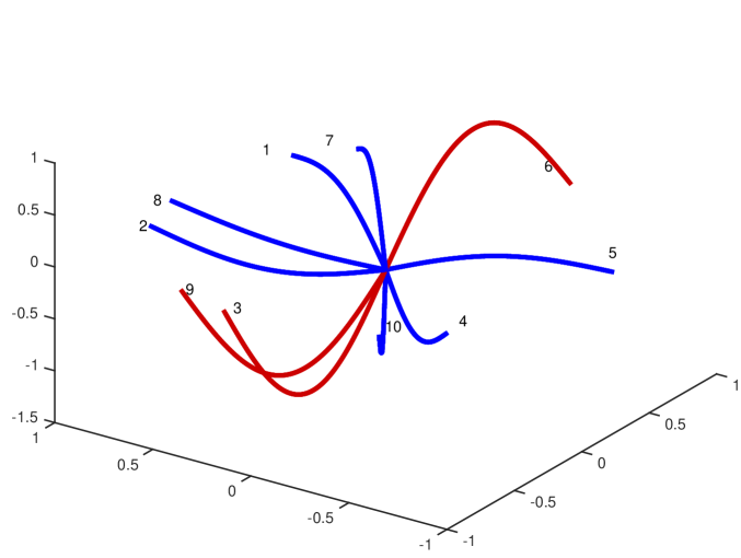
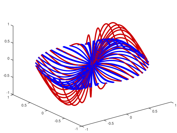
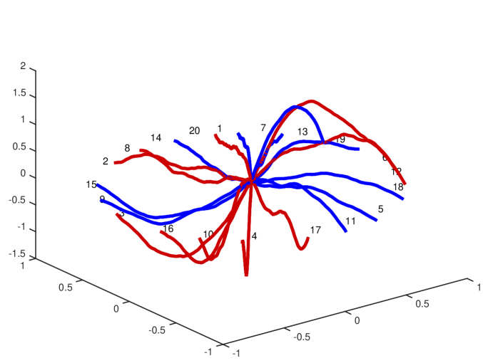
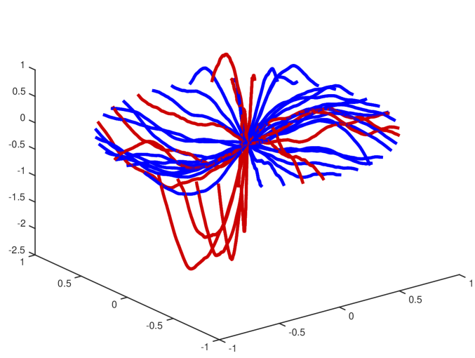
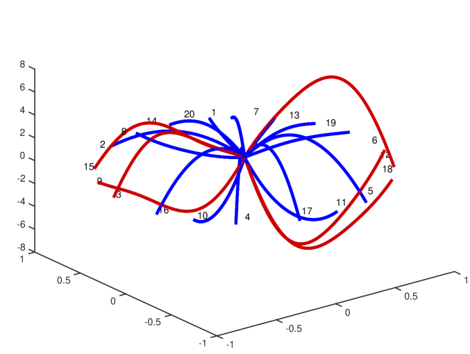
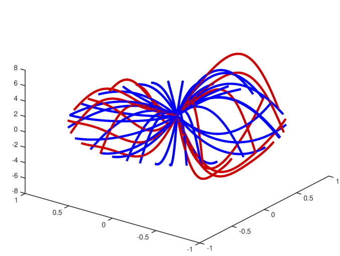
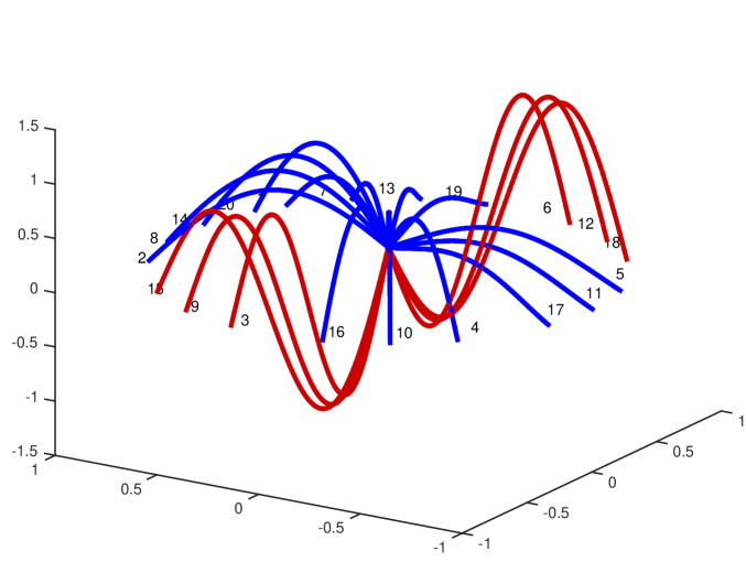
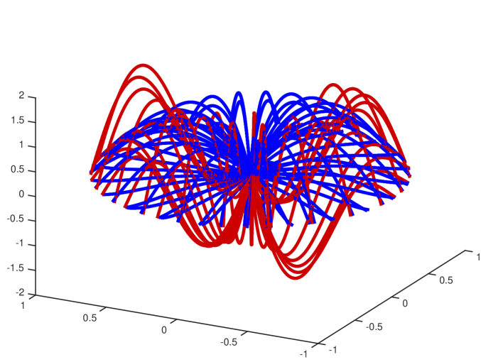
For all the examples we use the forcing terms $h^{n}=0$ for every $n\in\bm{\mathbbm{N}}$. The FEM approximation is done with $100$ elements per edge with uniform grid. For each example we present two graphics for values of $n$ chosen from $\{10,20,50,100,500,1000\}$, based on optical neatness. For visual purposes in all the cases the edges are colored with red if $K(e)=1$ or blue if $K(e)=2$. Also, for displaying purposes, in the cases $n\in\{10,20\}$ the edges $v_{\ell}v_{0}$ are labeled with “$\ell\,$” for identification, however for $n\in\{50,100,500,1000\}$ the labels were removed because they overload the image.

5.2 Verification Examples

Example 1 (A Riemann Integrable Forcing Term)

We begin our examples with the most familiar context as discussed in Remark 5. Define $F:\Omega\rightarrow\bm{\mathbbm{R}}$ by $F(t\cos\ell,t\sin\ell)\overset{\mathbf{def}}{=}\pi^{2}\,\sin(\pi t)\cos(\ell)$. Since both sequences $\{v_{\ell}:\ell\in\bm{\mathbbm{N}},\ell\equiv 0\mod 3\}$ and $\{v_{\ell}:\ell\in\bm{\mathbbm{N}},\ell\not\equiv 0\mod 3\}$ are equidistributed, Weyl’s Theorem 2 implies

$$\accentset{\rule{2.79996pt}{0.5pt}}{F}_{1}=\operatorname*{m_{\theta}}[F|_{\Omega_{G}^{1}}]=\accentset{\rule{2.79996pt}{0.5pt}}{F}_{2}=\operatorname*{m_{\theta}}[F|_{\Omega_{G}^{2}}]=\operatorname*{m_{\theta}}[F]\equiv 0.$$

Here $\accentset{\rule{2.79996pt}{0.5pt}}{F}_{1}$, $\accentset{\rule{2.79996pt}{0.5pt}}{F}_{2}$ are the limits defined in Hypothesis 2-(ii). For this case the exact solution of the upscaled Problem (26) is given by $\accentset{\rule{2.79996pt}{0.5pt}}{p}\overset{\mathbf{def}}{=}\accentset{\rule{2.79996pt}{0.5pt}}{p}\,\bm{\mathbbm{1}}_{\sigma_{1}}+\accentset{\rule{2.79996pt}{0.5pt}}{p}\,\bm{\mathbbm{1}}_{\sigma_{2}}\in H_{0}^{1}({\mathcal{G}})$, with $\accentset{\rule{2.79996pt}{0.5pt}}{p}_{1}(t)=\accentset{\rule{2.79996pt}{0.5pt}}{p}_{2}(t)=0$. For the diffusion coefficient we use the deterministic one, $K_{d}$ defined in (33a). The following table summarizes the convergence behavior.

Example 1 : Convergence Table, $K=K_{d}$.

$n$	$\|\accentset{\rule{2.79996pt}{0.5pt}}{p}^{\,n}_{1}-\accentset{\rule{2.79996pt}{0.5pt}}{p}_{1}\|_{L^{2}(_{e_{1}})}$	$\|\accentset{\rule{2.79996pt}{0.5pt}}{p}^{\,n}_{2}-\accentset{\rule{2.79996pt}{0.5pt}}{p}_{2}\|_{L^{2}(e_{1})}$	$\|\accentset{\rule{2.79996pt}{0.5pt}}{p}^{\,n}_{1}-\accentset{\rule{2.79996pt}{0.5pt}}{p}_{1}\|_{H^{1}_{0}(e_{2})}$	$\|\accentset{\rule{2.79996pt}{0.5pt}}{p}^{\,n}_{2}-\accentset{\rule{2.79996pt}{0.5pt}}{p}_{2}\|_{H^{1}_{0}(e_{2})}$
10	0.3526	0.1717	0.8232	0.3216
20	0.0180	0.0448	0.0900	0.0889
100	0.0160	0.0059	0.0395	0.0116
1000	$5.8352\times 10^{-4}$	$8.27772\times 10^{-4}$	0.0012	0.0016

(a) Solution $p^{10}$, $n=10$.

(b) Solution $p^{100}$, $n=100$.

Figure 3: Solutions Example 1. Diffusion coefficient $K_{d}$, see (33a). The solutions depicted in figures (a) and (b) on the edges $v_{\ell}v_{0}$ are colored with red if $K_{d}(v_{\ell}v_{0})=1$ (i.e., $\ell\equiv 0\mod 3$), or blue if $K_{d}(v_{\ell}v_{0})=2$ (i.e., $\ell\not\equiv 0\mod 3$). Forcing term $F:\Omega\rightarrow\bm{\mathbbm{R}}$, $F(t\cos\ell,t\sin\ell)\overset{\mathbf{def}}{=}\pi^{2}\,\sin(\pi t)\cos(\ell)$.

Example 2 (Probabilistic Flexibilities for Example 1)

This experiment follows the observations of Remark 6. In this case take $X\overset{\mathbf{def}}{=}K_{p}$, defined in (33b). Let $Z:\bm{\mathbbm{N}}\rightarrow[-100,100]$ be a random variable with uniform distribution and define $Y:\Omega_{G}\rightarrow\bm{\mathbbm{R}}$ by $Y(t\cos\ell,t\sin\ell)\overset{\mathbf{def}}{=}\pi^{2}\,\sin(\pi t)\cos(\ell)+Z(\ell)$. It is direct to see that $X$ and $Y$ satisfy Hypothesis 2 and due to the Law of Large Numbers, they also satisfy (31) and (32) respectively. Therefore

$$\accentset{\rule{2.79996pt}{0.5pt}}{Y}_{1}=\operatorname*{m_{\theta}}[F|_{\Omega_{G}^{1}}]=\accentset{\rule{2.79996pt}{0.5pt}}{Y}_{2}=\operatorname*{m_{\theta}}[F|_{\Omega_{G}^{2}}]=\operatorname*{m_{\theta}}[F]=\accentset{\rule{2.79996pt}{0.5pt}}{p}_{1}=\accentset{\rule{2.79996pt}{0.5pt}}{p}_{2}=0.$$

The following table is the summary for a fixed realization of $X$ (to keep the edge coloring consistent) and different realizations of $Y$ on each stage. Convergence is observed, as expected it is slower than in the previous case. This would also occur for different realizations of $X$ and $Y$ simultaneously.

Example 2: Convergence Table, $K=K_{p}$.

$n$	$\|\accentset{\rule{2.79996pt}{0.5pt}}{p}^{\,n}_{1}-\accentset{\rule{2.79996pt}{0.5pt}}{p}_{1}\|_{L^{2}(e_{1})}$	$\|\accentset{\rule{2.79996pt}{0.5pt}}{p}^{\,n}_{2}-\accentset{\rule{2.79996pt}{0.5pt}}{p}_{2}\|_{L^{2}(e_{1})}$	$\|\accentset{\rule{2.79996pt}{0.5pt}}{p}^{\,n}_{1}-\accentset{\rule{2.79996pt}{0.5pt}}{p}_{1}\|_{H^{1}_{0}(e_{2})}$	$\|\accentset{\rule{2.79996pt}{0.5pt}}{p}^{\,n}_{2}-\accentset{\rule{2.79996pt}{0.5pt}}{p}_{2}\|_{H^{1}_{0}(e_{2})}$
10	0.5534	0.0938	1.6629	0.5381
20	0.0965	0.1594	0.5186	0.3761
100	0.0653	0.1322	0.3809	0.2569
1000	0.0201	0.0302	0.0658	0.0597

(a) Solution $p^{20}$, $n=20$.

(b) Solution $p^{50}$, $n=50$.

Figure 4: Solutions of Example 2 Fixed realization of diffusion coefficient $K_{p}$, see (33b). Forcing term $Y:\Omega_{G}\rightarrow\bm{\mathbbm{R}}$, $Y(t\cos\ell,t\sin\ell)\overset{\mathbf{def}}{=}\pi^{2}\,\sin(\pi t)\cos(\ell)+Z(\ell)$, with $Z:\bm{\mathbbm{N}}\rightarrow[-100,100]$, random variable and $Z\sim\text{uniformly}$. Different realizations for $Y$ on each stage. The solutions depicted in figures (a) and (b) on the edges $v_{\ell}v_{0}$ are colored with red if $K_{p}(v_{\ell}v_{0})=1$ ($\operatorname*{\bm{\mathbbm{E}}}[K_{p}=1]=\frac{1}{3}$), or blue colored if $K_{p}(v_{\ell}v_{0})=2$ ($\operatorname*{\bm{\mathbbm{E}}}[K_{p}=2]=\frac{2}{3}$).

Example 3 (A non-Riemann Integrable Forcing Term)

For our final theoretical example we use a non-Riemann Integrable forcing term. Moreover, the following function is highly oscillatory inside each subdomain $\Omega_{G}^{1}$ and ${\Omega_{G}^{2}}$, and it can not be seen as Riemann integrable when restricted to any of the sub-domains. Let $F:\Omega_{G}\rightarrow\bm{\mathbbm{R}}$ be defined by

$$F(t\cos\ell,t\sin\ell)\overset{\mathbf{def}}{=}\begin{cases}4\pi^{2}\,\sin(2\pi t)+(-1)^{\lfloor\frac{\ell}{6}\rfloor}\times 10\times(\ell-\big{\lfloor}\frac{\ell}{2\pi}\big{\rfloor}),&\ell\equiv 0\mod 3,\\ \pi^{2}\,\sin(\pi t)+(-1)^{\lfloor\frac{\ell}{6}\rfloor}\times 10\times(\ell-\big{\lfloor}\frac{\ell}{2\pi}\big{\rfloor}),&\ell\not\equiv 0\mod 3.\end{cases}$$ (34)

On one hand, both sequences $\{v_{\ell}:\ell\in\bm{\mathbbm{N}},\ell\equiv 0\mod 3\}$ and $\{v_{\ell}:\ell\in\bm{\mathbbm{N}},\ell\not\equiv 0\mod 3\}$ are equidistributed. On the other hand both parts of the forcing term, the radial and the angular are Cesàro convergent on each $\Omega_{G}^{i}$ for $i=1,2$. The Cesàro average of the angular summand is zero on $\Omega_{G}^{i}$ for $i=1,2$. In contrast, the radial summand can be seen as Riemann integrable separately on each $\Omega_{G}^{i}$ for $i=1,2$, therefore, due to Weyl’s Theorem 2 its Cesàro average is given by $\accentset{\rule{2.79996pt}{0.5pt}}{F}_{1}=\operatorname*{m_{\theta}}[F|_{\Omega_{G}^{1}}]$ and $\accentset{\rule{2.79996pt}{0.5pt}}{F}_{2}=\operatorname*{m_{\theta}}[F|_{\Omega_{G}^{2}}]$; more explicitly,

$$\accentset{\rule{2.79996pt}{0.5pt}}{F}_{1}(t)=(2\pi)^{2}\sin(2\pi t)\,, \accentset{\rule{2.79996pt}{0.5pt}}{F}_{2}(t)=\pi^{2}\,\sin(\pi t).$$ (35)

For this case the exact solution $\accentset{\rule{2.79996pt}{0.5pt}}{p}=\accentset{\rule{2.79996pt}{0.5pt}}{p}\,\bm{\mathbbm{1}}_{\sigma_{1}}+\accentset{\rule{2.79996pt}{0.5pt}}{p}\,\bm{\mathbbm{1}}_{\sigma_{2}}\in H_{0}^{1}(-1,1)$ of the upscaled Problem (26) is given by

$$\accentset{\rule{2.79996pt}{0.5pt}}{p}_{1}(t)=\sin(2\pi t)\,, \accentset{\rule{2.79996pt}{0.5pt}}{p}_{2}(t)=\frac{1}{2}\,\sin(\pi t).$$ (36)

We summarize the convergence behavior in the table below.

Example 3: Convergence Table, $K=K_{d}$.

$n$	$\|\accentset{\rule{2.79996pt}{0.5pt}}{p}^{\,n}_{1}-\accentset{\rule{2.79996pt}{0.5pt}}{p}_{1}\|_{L^{2}(e_{1})}$	$\|\accentset{\rule{2.79996pt}{0.5pt}}{p}^{\,n}_{2}-\accentset{\rule{2.79996pt}{0.5pt}}{p}_{2}\|_{L^{2}(e_{1})}$	$\|\accentset{\rule{2.79996pt}{0.5pt}}{p}^{\,n}_{1}-\accentset{\rule{2.79996pt}{0.5pt}}{p}_{1}\|_{H^{1}_{0}(e_{2})}$	$\|\accentset{\rule{2.79996pt}{0.5pt}}{p}^{\,n}_{2}-\accentset{\rule{2.79996pt}{0.5pt}}{p}_{2}\|_{H^{1}_{0}(e_{2})}$
10	1.6392	0.4900	5.7447	1.3210
20	0.4127	0.9305	1.8930	1.7782
100	0.2125	0.3312	0.4986	0.6275
1000	0.0138	0.0189	0.0852	0.0371

(a) Solution $p^{20}$, $n=20$.

(b) Solution $p^{50}$, $n=50$.

Figure 5: Solutions of Example 3 Diffusion coefficient $K_{d}$, see (33a). The solutions depicted in figures (a) and (b) on the edges $v_{\ell}v_{0}$ are colored with red if $K_{d}(v_{\ell}v_{0})=1$ (i.e., $\ell\equiv 0\mod 3$), or blue if $K_{d}(v_{\ell}v_{0})=2$ (i.e., $\ell\not\equiv 0\mod 3$). Forcing term $F:\Omega_{G}\rightarrow\bm{\mathbbm{R}}$ see (34).

5.3 Numerical Experimentation Examples

In this section we present two examples, breaking different hypotheses of those required in the theoretical analysis discussed above. As there is not a known exact solution, we follow Cauchy’s convergence criterion for the sequences $\{\accentset{\rule{2.79996pt}{0.5pt}}{p}^{\,n}_{i}:n\in\bm{\mathbbm{N}}\}$ with $i=1,2$. However, we do not sample only points but intervals of observation and report the averages of the observed data. More specifically

$$\epsilon^{n}_{i}\overset{\mathbf{def}}{=}\frac{1}{10}\sum_{j=n-4}^{n+5}\|\accentset{\rule{2.79996pt}{0.5pt}}{p}^{\,j}_{i}-\accentset{\rule{2.79996pt}{0.5pt}}{p}^{\,j-1}_{i}\|_{L^{2}(e_{i})} \delta^{n}_{i}\overset{\mathbf{def}}{=}\frac{1}{10}\sum_{j=n-4}^{n+5}\|\accentset{\rule{2.79996pt}{0.5pt}}{p}^{\,j}_{i}-\accentset{\rule{2.79996pt}{0.5pt}}{p}^{\,j-1}_{i}\|_{H^{1}(e_{i})},$$ and

for $$i=1,2\,,\;n=10,20,100,1000.$$

Example 4 (A Locally Unbounded Forcing Term)

For our experiment we use a variation of Example 3, keeping the well-behaved radial part but adding an unbounded angular part, which is known to be Cesàro convergent to zero. Consider the forcing term $F:\Omega_{G}\rightarrow\bm{\mathbbm{R}}$ defined by

$$F(t\cos\ell,t\sin\ell)\overset{\mathbf{def}}{=}\begin{cases}4\pi^{2}\,\sin(2\pi t)+(-1)^{\ell}\sqrt{\ell}\,,&\ell\equiv 0\mod 3,\\ \pi^{2}\,\sin(\pi t)+(-1)^{\ell}\sqrt{\ell}\,,&\ell\not\equiv 0\mod 3.\end{cases}$$ (37)

Clearly, $\sup_{e\in E}\|F\|_{L^{2}(e)}=\infty$ i.e., Hypothesis 1-(i) is not satisfied. It is not hard to adjust the techniques presented in Section 4.1 to this case, when the forcing term is Cesàro convergent without satisfying the condition $\sup_{e\in E}\|F\|_{L^{2}(e)}=\infty$; however the properties of edgewise uniform convergence of Section 3.2 can not be concluded. Consequently, we observe the following convergence behavior.

Example 4: Convergence Table, $K=K_{d}$.

$n$	$\epsilon^{n}_{1}$	$\epsilon^{n}_{2}$	$\delta^{n}_{1}$	$\delta^{n}_{2}$
10	0.1547	0.1578	2.7336	2.7338
20	0.0618	0.0645	1.0734	1.0747
100	0.0277	0.0224	0.3394	0.3320
1000	0.0086	0.0065	0.0984	0.0955

(a) Solution $p^{20}$, $n=20$.

(b) Solution $p^{100}$, $n=100$.

Figure 6: Solutions of Example 4 Diffusion coefficient $K_{d}$, see (33a). The solutions depicted in figures (a) and (b) on the edges $v_{\ell}v_{0}$ are colored with red if $K_{d}(v_{\ell}v_{0})=1$ (i.e., $\ell\equiv 0\mod 3$), or blue if $K_{d}(v_{\ell}v_{0})=2$ (i.e., $\ell\not\equiv 0\mod 3$). Forcing term $F:\Omega_{G}\rightarrow\bm{\mathbbm{R}}$ see (37).

Example 5 (A Forcing Term with Unbounded Frequency Modes)

For our last experiment we use a variation of Example 3, keeping it bounded, but introducing unbounded frequencies. Consider the forcing term $F:\Omega_{G}\rightarrow\bm{\mathbbm{R}}$ defined by

$$F(t\cos\ell,t\sin\ell)\overset{\mathbf{def}}{=}\begin{cases}4\pi^{2}\,\sin(2\pi t\cdot\ell)\,,&\ell\equiv 0\mod 3,\\ \pi^{2}\,\sin(\pi t\cdot\ell)\,,&\ell\not\equiv 0\mod 3.\end{cases}$$ (38)

Clearly, $F$ verifies Hypothesis 1 , then Lemma 3 implies edgewise uniform convergence of the solutions, however Hypothesis-(ii) 2 is not satisfied. Therefore, we observe that the whole sequence is not Cauchy, although it has Cauchy subsequences as the following table shows.

Example 5: Convergence Table, $K=K_{d}$.

$n$	$\epsilon^{n}_{1}$	$\epsilon^{n}_{2}$	$\delta^{n}_{1}$	$\delta^{n}_{2}$
10	0.0264	0.0267	0.4157	0.3835
20	0.0078	0.0089	0.1342	0.1327
100	0.0004	0.0005	0.0077	0.0076
500	0.00004	0.00004	0.00073	0.00072
1000	0.00066	0.00049	0.0081	0.0078
1200	0.00004	0.00005	0.000787	0.000786

(a) Solution $p^{500}$, $n=500$.

(b) Solution $p^{1000}$, $n=1000$.

Figure 7: Solutions of Example 5. The Diffusion coefficient $K_{d}$, see (33a). The solutions depicted in figures (a) and (b) on the edges $v_{\ell}v_{0}$ are colored with red if $K_{d}(v_{\ell}v_{0})=1$ (i.e., $\ell\equiv 0\mod 3$), or blue if $K_{d}(v_{\ell}v_{0})=2$ (i.e., $\ell\not\equiv 0\mod 3$). Forcing term $F:\Omega_{G}\rightarrow\bm{\mathbbm{R}}$ see (38).

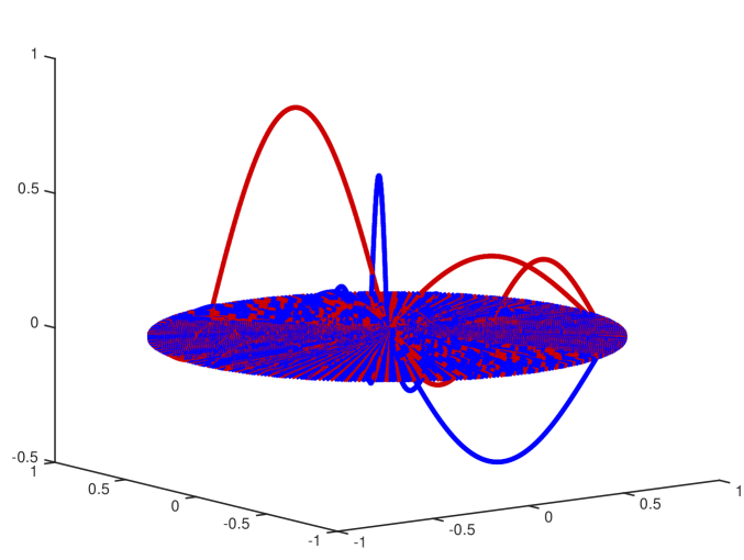
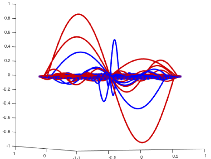
It follows that this system has more than one internal equilibrium. Consequently, an upscaled model of a system such as this, should contain uncertainty which, in this specific case, remains bounded due to the properties of the forcing term $F$.

5.4 Closing Observations

1. The authors tried to find experimentally a rate of convergence using the well-know estimate

   $$\alpha_{i}\sim\frac{\log\|\accentset{\rule{2.79996pt}{0.5pt}}{p}^{\,n+1}_{i}-\accentset{\rule{2.79996pt}{0.5pt}}{p}^{\,n}_{i}\|-\log\|\accentset{\rule{2.79996pt}{0.5pt}}{p}^{\,n}_{i}-\accentset{\rule{2.79996pt}{0.5pt}}{p}^{\,n-1}_{i}\|}{\log\|\accentset{\rule{2.79996pt}{0.5pt}}{p}^{\,n}_{i}-\accentset{\rule{2.79996pt}{0.5pt}}{p}^{\,n-1}_{i}\|-\log\|\accentset{\rule{2.79996pt}{0.5pt}}{p}^{\,n-1}_{i}-\accentset{\rule{2.79996pt}{0.5pt}}{p}^{\,n-2}_{i}\|}\,, i=1,2.$$

   The sampling was made on the intervals $n-5\leq j\leq n+5$, for $n=10,20,100,500$ and $1000$. Experiments were run on all the examples except for Example 5. In none of the cases, solid numerical evidence was detected that could suggest an order of convergence for the phenomenon.

2. Experiments for random variations of the examples above were also executed, under the hypothesis that random variables were subject to the Law of Large Numbers. Convergence, slower than its corresponding deterministic version was observed, as expected. This is important for its applicability to upscaling networks derived from game theory, see [20].

6 Conclusions and Final Discussion

The present work yields several accomplishments and also limitations as we point out below.

1. The method presented in this paper can be easily extended to general scale-free networks in a very simple way. First identify the communication kernel (see [13]). Second, for each node in the kernel, replace its numerous incident low-degree nodes by the upscaled nodes together with the homogenized diffusion coefficients and forcing terms, see Figure 1.

2. The particular scale-free network treated in the paper i.e., the star metric graph, arises naturally in some important examples. These come from the theory of the strategic network formation, where the agents choose their connections following utilitarian behavior. Under certain conditions for the benefit-cost relation affecting the actors when establishing links with other agents, the asymptotic network is star-shaped (see [21]).

3. The scale-free networks are frequent in many real world examples as already mentioned. It follows that the method is applicable to a wide range of cases. However, important networks can not be treated the same way for homogenization, even if they share some important properties of communication. The small-world networks constitute an example since they are highly clustered, this feature contradicts the power-law degree distribution hypothesis. See [22] for a detailed exposition on the matter.

4. The upscaling of the diffusion phenomenon is done in a hybrid fashion. On one hand, the diffusion on the low-degree nodes is modeled by the weak variational form of the differential operators defined over the graph, but ignoring its combinatorial structure. On the other hand, the diffusion on the communication kernel will still depend on both, the differential operators and the combinatorial structure. This is an important achievement, because it is consistent with the nature of available data for the analysis of real world networks. Typically, the data for central (or highly connected) agents are more reliable than data for marginal (or low degree) agents.

5. The central Cesàro convergence hypotheses for data behavior (stated in Lemma 3-(iii), as well as those contained in Hypothesis 2, in order to conclude convergence have probabilistic-statistical nature. This is one of the main accomplishments of the work, because the hypotheses are mild and adjust to realistic scenarios; unlike strong hypotheses of topological nature such as periodicity, continuity, differentiability or even Riemann-integrability of the forcing terms (see [11]). This fact is further illustrated in Example 3, where good asymptotic behavior is observed for a forcing term which is nowhere continuous on the domain $\Omega_{G}$ of analysis.

6. An important and desirable consequence of the data hypotheses adopted, is that the method can be extended to more general scenarios, as mentioned in Remark 6, reported in Subsection 5.4 and illustrated in Examples 2, 4 and 5. Moreover, Example 5 suggests a probabilistic upscaled model for the communication kernel, to be explored in future work.

7. A different line of future research consists in the analysis of the same phenomenon, but using the mixed-mixed variational formulation introduced in [23] instead of the direct one used in the present analysis. The key motivation in doing so, is that the mixed-mixed formulation is capable of modeling more general exchange conditions than those handled by the direct variational formulation and by the classic mixed formulations. This advantage can broaden in a significant way the spectrum of real-world networks which can be successfully modeled and upscaled.

8. Finally, the preexistent literature typically analyses the asymptotic behavior of diffusion in complex networks, starting from fully discrete models (e.g., [24, 25]). The pseudo-discrete treatment that we have followed here, constitutes more a complementary than an alternative approach. Depending on the availability of data and/or sampling, as well as the scale of interest for a particular problem, it is natural to consider a “blending” of both techniques.

References

- [1] A.-L. Barabási, R. Albert, Emergence of scaling in random networks, Science 286 (1999) 509–512.
- [2] R. Kumar, P. Raghavan, S. Rajagopalan, D. Sivakumar, A. Tompkins, E. Upfal, Stochastic models for the web graph, FOCS: IEES Symposium on Foundations of Computer Science (2000) 57–66.
- [3] S. Wuchty, Scale-free behavior in protein domain networks, Molecular Biology and Evolution 18 (2001) 1694–1702.
- [4] M. Faloutsos, P. Faloutsos, C. Faloutsos, On power-law relationships of the internet topology, Computer Communication Review 29 (1999) 251–262.
- [5] S. Bortoluzzi, C. Romualdi, A. Bisognin, G. A. Danielli, Disease genes and intracelullar protein networks, Physiol. Genom. 15 (2003) 223–227.
- [6] P. Tsaparas, L. M. Ramírez, O. Bodenreider, E. V. Kooning, I. Jordan, Global similarity and local divergence in human and mouse gene coexpression networks, BMC Evol. Biol. 6 (2006) 70. doi:10.1186/1471-2148-6-70.
- [7] E. F. Keller, Revisiting “scale-free” networks, BioEssay 27 (2005) 1060–1068. doi:10.1002/bies.20294.
- [8] L. Li, D. Alderson, W. Wilinger, J. Doyle, A first-principles approch to understanding the internet’s router-level topology, Computer Communication Review 34(4) (2004) 3–14.
- [9] D. M. Kreps, Microeconomic Foundations I, Choice and Competitive Markets, Princeton University Press, Princeton, NJ, 2013.
- [10] D. Cioranescu, P. Donato, An Introduction to Homogenization, Oxford Series in Mathematics and its Applications, Vol 17, Oxford University Press, NY, 1999.
- [11] U. Hornung, Homogenization and Porous Media, Vol. 6 of Interdisciplinary Applied Mathematics, Springer-Verlag, New York, 1997.
- [12] E. Estrada, The Structure of Complex Networks, Theory and Applications, Oxford University Press, New York, 2012.
- [13] D.-H. Kim, J. D. Noh, H. Jeong, Scale-free trees: The skeletons of complex networks, Physical Review E 70 (2004) 0416126. doi:10.113/PhysRevE.70.046126.
- [14] G. Berkolaiko, P. Kuchment, Introduction to Quantum Graphs, Mathematical Surveys and Monographs, Vol 186, American Mathematical Society, Providence, RI, 2013.
- [15] J. M. Ramírez, Population persistence under advection-diffusion in river networks, Journal of Mathematical Biology 65(5) (2011) 919–942. doi:10.1007/s00285-011-0485-6.
- [16] I. Farý, On the straight line representations of planar graphs, Acta Sci. Math. 11 (1948) 229–233.
- [17] A. Bondy, U. Murty, Graph Theory, Graduate Texts in Mathematics, vol. 244, Springer, 2008.
- [18] E. M. Stein, R. Shakarchi, Fourier Analysis. An Introduction, Princeton Lectures in Analysis, Princeton University Press, Princeton, NJ, 2003.
- [19] M. Peszyǹska, fem1d.m: Template for solving a two point boundary value problem, Library, http://www.math.oregonstate.edu/~mpesz/code/teaching.html (2008–2015).
- [20] M. O. Jackson, Social and Economic Networks, Princeton University Press, Princeton, NJ, 2008.
- [21] M. O. Jackson, F. Bloch, The formation of networks with transfers among players, Journal of Economic Theory 133(1) (2007) 83–110.
- [22] M. O. Jackson, B. W. Rogers, The economics of small worlds, Journal of the European Economic Association 2(3) (2005) 617–627.
- [23] F. Morales, R. Showalter, Interface approximation of Darcy flow in a narrow channel., Mathematical Methods in the Applied Sciences 35 (2012) 182–195.
- [24] M. O. Jackson, L. Yariv, Diffusion on social networks, Économie Publique 1 (1) (2005) 3–16.
- [25] M. O. Jackson, D. López-Pintado, Diffusion and contagion in networks with heterogenous agents and homophily, Network Science 1 (1) (20013) 49–77.