Efficiency of Z๐‘Z-estimators indexed by the objective functions

Franรงois Portier111Universitรฉ catholique de Louvain, Institut de Statistique, Biostatistique et Sciences Actuarielles, Voie du Roman Paysย 20, B-1348 Louvain-la-Neuve, Belgium. E-mail: {francois.portier}@uclouvain.be. This work has been supported by Fonds de la Recherche Scientifique (FNRS) A4/5 FC 2779/2014-2017 No.ย 22342320.
Abstract

We study the convergence of Z๐‘Z-estimators ฮธ^โ€‹(ฮท)โˆˆโ„p^๐œƒ๐œ‚superscriptโ„๐‘\widehat{\theta}(\eta)\in\mathbb{R}^{p} for which the objective function depends on a parameter ฮท๐œ‚\eta that belongs to a Banach space โ„‹โ„‹\mathcal{H}. Our results include the uniform consistency over โ„‹โ„‹\mathcal{H} and the weak convergence in the space of bounded โ„psuperscriptโ„๐‘\mathbb{R}^{p}-valued functions defined on โ„‹โ„‹\mathcal{H}. Furthermore when ฮท๐œ‚\eta is a tuning parameter optimally selected at ฮท0subscript๐œ‚0\eta_{0}, we provide conditions under which an estimated ฮท^^๐œ‚\widehat{\eta} can be replaced by ฮท0subscript๐œ‚0\eta_{0} without affecting the asymptotic variance. Interestingly, these conditions are free from any rate of convergence of ฮท^^๐œ‚\widehat{\eta} to ฮท0subscript๐œ‚0\eta_{0} but they require the space described by ฮท^^๐œ‚\widehat{\eta} to be not too large. We highlight several applications of our results and we study in detail the case where ฮท๐œ‚\eta is the weight function in weighted regression.

Keywords: Z๐‘Z-estimators, efficiency, weighted regression, empirical process.

1 Introduction

Let P๐‘ƒP denote a probability measure defined on a measurable space (๐’ต,๐’œ)๐’ต๐’œ(\mathcal{Z},\mathcal{A}) and let (Z1,โ€ฆ,Zn)subscript๐‘1โ€ฆsubscript๐‘๐‘›(Z_{1},\ldots,Z_{n}) be independent and identically distributed random elements with law P๐‘ƒP. Given a measurable function f:๐’ตโ†’โ„:๐‘“โ†’๐’ตโ„f:\mathcal{Z}\rightarrow\mathbb{R}, we define

Pโ€‹f=โˆซfโ€‹๐‘‘P,โ„™nโ€‹f=nโˆ’1โ€‹โˆ‘i=1nfโ€‹(Zi),๐”พnโ€‹f=n1/2โ€‹(โ„™nโˆ’P)โ€‹f,formulae-sequence๐‘ƒ๐‘“๐‘“differential-d๐‘ƒformulae-sequencesubscriptโ„™๐‘›๐‘“superscript๐‘›1superscriptsubscript๐‘–1๐‘›๐‘“subscript๐‘๐‘–subscript๐”พ๐‘›๐‘“superscript๐‘›12subscriptโ„™๐‘›๐‘ƒ๐‘“\displaystyle Pf=\int fdP,\qquad\mathbb{P}_{n}f=n^{-1}\sum_{i=1}^{n}f(Z_{i}),\qquad\mathbb{G}_{n}f=n^{1/2}(\mathbb{P}_{n}-P)f,

where ๐”พnsubscript๐”พ๐‘›\mathbb{G}_{n} is called the empirical process. Considering the estimation of a Euclidean parameter ฮธ0โˆˆฮ˜โŠ‚โ„psubscript๐œƒ0ฮ˜superscriptโ„๐‘\theta_{0}\in\Theta\subset\mathbb{R}^{p}, let (โ„‹,โˆฅโ‹…โˆฅ)(\mathcal{H},\|\cdot\|) denote a Banach space and let {ฮธ^โ€‹(ฮท):ฮทโˆˆโ„‹}conditional-set^๐œƒ๐œ‚๐œ‚โ„‹\{\widehat{\theta}(\eta)\ :\ \eta\in\mathcal{H}\} be a collection of estimators of ฮธ0subscript๐œƒ0\theta_{0} based on the sample (Z1,โ€ฆ,Zn)subscript๐‘1โ€ฆsubscript๐‘๐‘›(Z_{1},\ldots,Z_{n}). Suppose furthermore that there exists ฮท0โˆˆโ„‹subscript๐œ‚0โ„‹\eta_{0}\in\mathcal{H} such that ฮธ^โ€‹(ฮท0)^๐œƒsubscript๐œ‚0\widehat{\theta}(\eta_{0}) is efficient within the collection, i.e., ฮธ^โ€‹(ฮท0)^๐œƒsubscript๐œ‚0\widehat{\theta}(\eta_{0}) has the smallest asymptotic variance among the estimators of the collection. Such a situation arises in many fields of the statistics. For instance, ฮท๐œ‚\eta can be the cut-off parameter in Huber robust regression, or ฮท๐œ‚\eta might as well be equal to the weight function in heteroscedastic regression (see the next section for more details and examples). Unfortunately, ฮท0subscript๐œ‚0\eta_{0} is generally unknown since it certainly depends on the model P๐‘ƒP. Usually, one is restricted to first estimate ฮท0subscript๐œ‚0\eta_{0} by, say, ฮท^^๐œ‚\widehat{\eta} and then compute the estimator ฮธ^โ€‹(ฮท^)^๐œƒ^๐œ‚\widehat{\theta}(\widehat{\eta}), which should result in a not too bad approximation of ฮธ0subscript๐œƒ0\theta_{0}. It turns out that in many different situations ฮธ^โ€‹(ฮท^)^๐œƒ^๐œ‚\widehat{\theta}(\widehat{\eta}) actually achieves the efficiency bound of the collection (see for instance Newey and McFadden (1994), page 2164, and the reference therein, or vanย der Vaart (1998), page 61). This is all the more surprising since the accuracy of ฮท^^๐œ‚\widehat{\eta} estimating ฮท0subscript๐œ‚0\eta_{0} does not matter provided its consistency.

A paradigm that encompasses the previous facts can be developed via the stochastic equicontinuity of the underlying empirical process. Define the process ฮทโ†ฆโ„คnโ€‹(ฮท)=nโ€‹(ฮธ^โ€‹(ฮท)โˆ’ฮธ0)maps-to๐œ‚subscriptโ„ค๐‘›๐œ‚๐‘›^๐œƒ๐œ‚subscript๐œƒ0\eta\mapsto\mathbb{Z}_{n}(\eta)=\sqrt{n}(\widehat{\theta}(\eta)-\theta_{0}) and assume that it lies in โ„“โˆžโ€‹(โ„‹)superscriptโ„“โ„‹\ell^{\infty}(\mathcal{H}), the space of bounded โ„psuperscriptโ„๐‘\mathbb{R}^{p}-valued functions defined on โ„‹โ„‹\mathcal{H}. It is stochastically equicontinuous on โ„‹โ„‹\mathcal{H} if for any ฯต>0italic-ฯต0\epsilon>0,

limฮดโ†’0lim supnโ†’+โˆžP(supโ€–ฮท1โˆ’ฮท2โ€–<ฮด|โ„คn(ฮท1)โˆ’โ„คn(ฮท2))|>ฯต)=0,\displaystyle\lim_{\delta\rightarrow 0}\limsup_{n\rightarrow+\infty}\ P\big{(}\ \sup_{\|\eta_{1}-\eta_{2}\|<\delta}|\mathbb{Z}_{n}(\eta_{1})-\mathbb{Z}_{n}(\eta_{2}))|>\epsilon\ \big{)}=0, (1)

where |โ‹…||\cdot| stands for the Euclidean norm. Clearly, ฮธ^โ€‹(ฮท^)^๐œƒ^๐œ‚\widehat{\theta}(\widehat{\eta}) is efficient whenever nโ€‹(ฮธ^โ€‹(ฮท^)โˆ’ฮธ^โ€‹(ฮท0))=โ„คnโ€‹(ฮท^)โˆ’โ„คnโ€‹(ฮท0)๐‘›^๐œƒ^๐œ‚^๐œƒsubscript๐œ‚0subscriptโ„ค๐‘›^๐œ‚subscriptโ„ค๐‘›subscript๐œ‚0\sqrt{n}(\widehat{\theta}(\widehat{\eta})-\widehat{\theta}(\eta_{0}))=\mathbb{Z}_{n}(\widehat{\eta})-\mathbb{Z}_{n}(\eta_{0}) goes to 00 in probability. This holds true if, in addition to (1), we have that

Pโ€‹(ฮท^โˆˆโ„‹)โŸถ1andโ€–ฮท^โˆ’ฮท0โ€–โ€‹โŸถ๐‘ƒโ€‹0.โŸถ๐‘ƒ^๐œ‚โ„‹1andnorm^๐œ‚subscript๐œ‚0๐‘ƒโŸถ0\displaystyle P(\widehat{\eta}\in\mathcal{H})\longrightarrow 1\qquad\text{and}\qquad\|\widehat{\eta}-\eta_{0}\|\overset{P}{\longrightarrow}0. (2)

In other words, stochastic equicontinuity allows for a โ€œno rateโ€ condition on ฮท^^๐œ‚\widehat{\eta} given in (2). In fact, conditions (1) and (2) represent a trade-off we need to accomplish when selecting the norm โˆฅโ‹…โˆฅ\|\cdot\|. When one prefers to have โˆฅโ‹…โˆฅ\|\cdot\| as weak as possible in order to prove (2), one needs the metric to be strong enough so that (1) can hold. In many statistical problems, one has

n1/2โ€‹(ฮธ^โ€‹(ฮท)โˆ’ฮธ0)=๐”พnโ€‹ฯ†ฮท+oPโ€‹(1),superscript๐‘›12^๐œƒ๐œ‚subscript๐œƒ0subscript๐”พ๐‘›subscript๐œ‘๐œ‚subscript๐‘œ๐‘ƒ1\displaystyle n^{1/2}(\widehat{\theta}(\eta)-\theta_{0})=\mathbb{G}_{n}\varphi_{\eta}+o_{P}(1),

where the oPโ€‹(1)subscript๐‘œ๐‘ƒ1o_{P}(1) is uniform over ฮทโˆˆโ„‹๐œ‚โ„‹\eta\in\mathcal{H} and ฯ†ฮทsubscript๐œ‘๐œ‚\varphi_{\eta} is a measurable function often called the influence function. This asymptotic decomposition permits to use empirical process theory and, in particular, the Donsker property in order to show (1) with โˆฅโ‹…โˆฅ\|\cdot\| being the L2โ€‹(P)subscript๐ฟ2๐‘ƒL_{2}(P)-norm. As it is summarized in vanย der Vaart and Wellner (1996), sufficient conditions deal with the metric entropy of the class of functions {ฯ†ฮท:ฮทโˆˆโ„‹}conditional-setsubscript๐œ‘๐œ‚๐œ‚โ„‹\{\varphi_{\eta}\ :\ \eta\in\mathcal{H}\} that needs to be small enough.

The main purpose of the paper is to establish general conditions for the efficiency of Z๐‘Z-estimators for which the objective function depends on some ฮทโˆˆโ„‹๐œ‚โ„‹\eta\in\mathcal{H}. More formally, we consider ฮธ0subscript๐œƒ0\theta_{0} and ฮธ^โ€‹(ฮท)^๐œƒ๐œ‚\widehat{\theta}(\eta) defined, respectively, as โ€œzerosโ€ of the maps

ฮธโ†ฆPโ€‹ฯˆฮทโ€‹(ฮธ)andฮธโ†ฆโ„™nโ€‹ฯˆฮทโ€‹(ฮธ),formulae-sequencemaps-to๐œƒ๐‘ƒsubscript๐œ“๐œ‚๐œƒandmaps-to๐œƒsubscriptโ„™๐‘›subscript๐œ“๐œ‚๐œƒ\displaystyle\theta\mapsto P\psi_{\eta}(\theta)\qquad\text{and}\qquad\theta\mapsto\mathbb{P}_{n}\psi_{\eta}(\theta),

where for each ฮธโˆˆฮ˜๐œƒฮ˜\theta\in\Theta and ฮทโˆˆโ„‹๐œ‚โ„‹\eta\in\mathcal{H}, ฯˆฮทโ€‹(ฮธ)subscript๐œ“๐œ‚๐œƒ\psi_{\eta}(\theta) is an โ„psuperscriptโ„๐‘\mathbb{R}^{p}-valued measurable map defined on ๐’ต๐’ต\mathcal{Z}. Since for every ฮทโˆˆโ„‹๐œ‚โ„‹\eta\in\mathcal{H}, Pโ€‹ฯˆฮทโ€‹(ฮธ0)=0๐‘ƒsubscript๐œ“๐œ‚subscript๐œƒ00P\psi_{\eta}(\theta_{0})=0, we have several (possibly infinitely many) equations that characterize ฮธ0subscript๐œƒ0\theta_{0}. Hence ฮท๐œ‚\eta can better be understood as a tuning parameter rather than as a classical nuisance parameter: ฮท๐œ‚\eta has no effect on the consistency of ฮธ^โ€‹(ฮท)^๐œƒ๐œ‚\widehat{\theta}(\eta) but it influences the asymptotic variance. In Newey (1994), similar semiparametric estimators are studied using pathwise derivatives along sub-models and the author underlines that, for such models, โ€œdifferent nonparametric estimators of the same functions should result in the same asymptotic varianceโ€ (Newey, 1994, page 1356). In Andrews (1994), the previous statement is formally demonstrated by relying on stochastic equicontinuity, as detailed in (1) and (2). In this paper, we provide new conditions on the map (ฮธ,ฮท)โ†ฆฯˆฮทโ€‹(ฮธ)maps-to๐œƒ๐œ‚subscript๐œ“๐œ‚๐œƒ(\theta,\eta)\mapsto\psi_{\eta}(\theta) and the estimators ฮท^^๐œ‚\widehat{\eta} under which the following statement holds: ฮธ^โ€‹(ฮท^)^๐œƒ^๐œ‚\widehat{\theta}(\widehat{\eta}) has the same asymptotic law as ฮธ^โ€‹(ฮท0)^๐œƒsubscript๐œ‚0\widehat{\theta}(\eta_{0}). Despite considering slightly less general estimators than in Andrews (1994), our approach alleviates the regularity conditions imposed on the map ฮธโ†ฆฯˆฮทโ€‹(ฮธ)maps-to๐œƒsubscript๐œ“๐œ‚๐œƒ\theta\mapsto\psi_{\eta}(\theta). They are replaced by weaker regularity conditions dealing with the map ฮธโ†ฆPโ€‹ฯˆฮทโ€‹(ฮธ)maps-to๐œƒ๐‘ƒsubscript๐œ“๐œ‚๐œƒ\theta\mapsto P\psi_{\eta}(\theta). Moreover, we focus on conditional moment restrictions models in which ฮท๐œ‚\eta is a weight function. In this context, our approach results in a very simple condition on the metric entropy generated by ฮท^^๐œ‚\widehat{\eta}, which is shown to be satisfied for classical Nadaraya-Watson estimators.

Our study is based on the weak convergence of {nโ€‹(ฮธ^โ€‹(ฮท)โˆ’ฮธ0)}ฮทโˆˆโ„‹subscript๐‘›^๐œƒ๐œ‚subscript๐œƒ0๐œ‚โ„‹\{\sqrt{n}(\widehat{\theta}(\eta)-\theta_{0})\}_{\eta\in\mathcal{H}} as a stochastic process belonging to โ„“โˆžโ€‹(โ„‹)superscriptโ„“โ„‹\ell^{\infty}(\mathcal{H}). To the best of our knowledge, this result is new. The tools we use in the proofs are reminiscent of the Z๐‘Z-estimation literature for which we mention several relevant contributions. In the case where ฮธ0subscript๐œƒ0\theta_{0} is Euclidean, asymptotic normality is obtained in Huber (1967). Nonsmooth objective functions are considered in Pollard (1985). In the case where ฮธ0subscript๐œƒ0\theta_{0} is infinite dimensional, weak convergence is established in vanย der Vaart (1995). The presence of a nuisance parameter with possibly, slower than root n๐‘›n rates of convergence, is studied in Newey (1994). Nonsmooth objective functions are investigated in Chen etย al. (2003). Relevant summaries might be found in the books Newey and McFadden (1994), vanย der Vaart and Wellner (1996), vanย der Vaart (1998).

Among the different applications we have in mind, we focus on weighted regression for heteroscedastic models. Even though this topic is quite well understood (see among others, Robinson (1987), Carroll etย al. (1988) and the references therein), it represents an interesting example to apply our results. In linear regression, given the data (Yi,Xi)i=1,โ€ฆ,nsubscriptsubscript๐‘Œ๐‘–subscript๐‘‹๐‘–๐‘–1โ€ฆ๐‘›(Y_{i},X_{i})_{i=1,\ldots,n}, where, for each i=1โ€‹โ€ฆ,n๐‘–1โ€ฆ๐‘›i=1\ldots,n, Yiโˆˆโ„subscript๐‘Œ๐‘–โ„Y_{i}\in\mathbb{R} is the response and Xiโˆˆโ„qsubscript๐‘‹๐‘–superscriptโ„๐‘žX_{i}\in\mathbb{R}^{q} are the covariates, it consists of computing

ฮฒ^โ€‹(w)=argminฮฒโ€‹โˆ‘i=1n(Yiโˆ’ฮฒTโ€‹Xi)2โ€‹wโ€‹(Xi),^๐›ฝ๐‘คsubscriptargmin๐›ฝsuperscriptsubscript๐‘–1๐‘›superscriptsubscript๐‘Œ๐‘–superscript๐›ฝ๐‘‡subscript๐‘‹๐‘–2๐‘คsubscript๐‘‹๐‘–\displaystyle\widehat{\beta}(w)=\operatorname{argmin}_{\beta}\sum_{i=1}^{n}(Y_{i}-\beta^{T}X_{i})^{2}w(X_{i}), (3)

where w๐‘คw denotes a real valued function. Among such a collection of estimators, there exists an efficient member ฮธ^โ€‹(w0)^๐œƒsubscript๐‘ค0\widehat{\theta}(w_{0}) (see section 4.1 for details). Many studies have focused on the estimation of w0subscript๐‘ค0w_{0}. For instance, Carroll and Ruppert (1982) argues that a parametric estimation of w0subscript๐‘ค0w_{0} can be performed, and Carroll (1982) and Robinson (1987) use different nonparametric estimators to approximate w0subscript๐‘ค0w_{0}. The estimators ฮฒ^โ€‹(w^)^๐›ฝ^๐‘ค\widehat{\beta}(\widehat{w}) are shown to be efficient by relying on U๐‘ˆU-statistics-based decompositions. It involves relatively long and peculiar calculations that depend on both w^^๐‘ค\widehat{w} and the loss function. Our approach overpass this issue by providing high-level conditions on w^^๐‘ค\widehat{w} that are in some ways independent from the rest of the problem. In summary we require that w^โ€‹(x)โ†’w0โ€‹(x)โ†’^๐‘ค๐‘ฅsubscript๐‘ค0๐‘ฅ\widehat{w}(x)\rightarrow w_{0}(x) in probability, dโ€‹Pโ€‹(x)๐‘‘๐‘ƒ๐‘ฅdP(x)-almost everywhere, and that there exists a function space ๐’ฒ๐’ฒ\mathcal{W} such that

Pโ€‹(w^โˆˆ๐’ฒ)โ†’1andโˆซ0+โˆžlogโก๐’ฉ[]โ€‹(ฯต,๐’ฒ,Lrโ€‹(P))โ€‹๐‘‘ฯต<+โˆž,formulae-sequenceโ†’๐‘ƒ^๐‘ค๐’ฒ1andsuperscriptsubscript0subscript๐’ฉitalic-ฯต๐’ฒsubscript๐ฟ๐‘Ÿ๐‘ƒdifferential-ditalic-ฯต\displaystyle P(\widehat{w}\in\mathcal{W})\rightarrow 1\qquad\text{and}\qquad\int_{0}^{+\infty}\sqrt{\log\mathcal{N}_{[\ ]}\big{(}\epsilon,\mathcal{W},L_{r}(P)\big{)}}d\epsilon<+\infty,

for some r>2๐‘Ÿ2r>2, where ๐’ฉ[]subscript๐’ฉ\mathcal{N}_{[\ ]} denotes the bracketing numbers as defined in vanย der Vaart and Wellner (1996). When w0subscript๐‘ค0w_{0} is modelled parametrically, the previous conditions are fairly easy to verify. For nonparametric estimators of w0subscript๐‘ค0w_{0}, in particular for Nadaraya-Watson estimators, smoothness restrictions on ๐’ฒ๐’ฒ\mathcal{W} with respect to the dimension q๐‘žq allows to obtain sufficiently sharp bounds on the bracketing number of ๐’ฒ๐’ฒ\mathcal{W}.

The paper is organised as follows. We describe in Section 2 several examples of estimators for which the efficiency might follow from our approach. Section 3 contains the theoretical background of the paper. We study the consistency and the weak convergence of ฮธ^โ€‹(ฮท)^๐œƒ๐œ‚\widehat{\theta}(\eta), ฮทโˆˆโ„‹๐œ‚โ„‹\eta\in\mathcal{H}. Based on this, we obtain conditions for the efficiency of ฮธ^โ€‹(ฮท^)^๐œƒ^๐œ‚\widehat{\theta}(\widehat{\eta}). At the end of Section 3, we consider weighted estimators for conditional moment restrictions models. In section 4, we are concerned about the estimation of the optimal weight function w0subscript๐‘ค0w_{0} in weighted linear regression. We investigate different approaches from the parametric to the fully nonparametric. In Section 5, we evaluate the finite sample performance of several methods by means of simulations.

2 Examples

As discussed in the introduction, the results of the paper allow to obtain the efficiency of estimators that depend on a tuning parameter. This occurs at different levels of statistical theory. We raise several examples in the following.

Example 1.

(Least-square constrained estimation) Given ฮธ^^๐œƒ\widehat{\theta} an arbitrary but consistent estimator of ฮธ0subscript๐œƒ0\theta_{0}, the estimator ฮธ^csubscript^๐œƒ๐‘\widehat{\theta}_{c} is said to be a least-square constraint estimator if it minimizes (ฮธโˆ’ฮธ^)Tโ€‹ฮ“โ€‹(ฮธโˆ’ฮธ^)superscript๐œƒ^๐œƒ๐‘‡ฮ“๐œƒ^๐œƒ(\theta-\widehat{\theta})^{T}\Gamma(\theta-\widehat{\theta}) over ฮธโˆˆฮ˜๐œƒฮ˜\theta\in\Theta, where ฮ“ฮ“\Gamma is lying over the set of symmetric positive definite matrices such that ฮ“โ‰ฅb>0ฮ“๐‘0\Gamma\geq b>0. Consequently ฮธ^csubscript^๐œƒ๐‘\widehat{\theta}_{c} depends on the choice of ฮ“ฮ“\Gamma but since |ฮธ^cโˆ’ฮธ^|2โ‰คbโˆ’1โ€‹|ฮ“1/2โ€‹(ฮธ^cโˆ’ฮธ^)|2โ‰คbโˆ’1โ€‹|ฮ“1/2โ€‹(ฮธ0โˆ’ฮธ^)|2โŸถ0superscriptsubscript^๐œƒ๐‘^๐œƒ2superscript๐‘1superscriptsuperscriptฮ“12subscript^๐œƒ๐‘^๐œƒ2superscript๐‘1superscriptsuperscriptฮ“12subscript๐œƒ0^๐œƒ2โŸถ0|\widehat{\theta}_{c}-\widehat{\theta}|^{2}\leq b^{-1}|\Gamma^{1/2}(\widehat{\theta}_{c}-\widehat{\theta})|^{2}\leq b^{-1}|\Gamma^{1/2}(\theta_{0}-\widehat{\theta})|^{2}\longrightarrow 0 in probability, the matrix ฮ“ฮ“\Gamma does not affect the consistency of ฮธ^csubscript^๐œƒ๐‘\widehat{\theta}_{c} estimating ฮธ0subscript๐œƒ0\theta_{0}. It is well known that ฮธ^csubscript^๐œƒ๐‘\widehat{\theta}_{c} is efficient whenever ฮ“ฮ“\Gamma equals the inverse of the asymptotic variance of ฮธ^^๐œƒ\widehat{\theta} (Newey and McFadden, 1994, Section 5.2). Such a class is popular among econometricians and known as minimal distance estimator.

In the above illustrative example, the use of the asymptotic equicontinuity of the process ฮ“โ†ฆnโ€‹(ฮธ^cโˆ’ฮธ0)maps-toฮ“๐‘›subscript^๐œƒ๐‘subscript๐œƒ0\Gamma\mapsto\sqrt{n}(\widehat{\theta}_{c}-\theta_{0}) is not really legitimate since we could obtain the efficiency using more basic tools such as the Slutskyโ€™s lemma in Euclidean space. This is due of course to the Euclideanity of ฮธ๐œƒ\theta and ฮ“ฮ“\Gamma but also to the simplicity of the map (ฮธ,ฮ“)โ†ฆ(ฮธโˆ’ฮธ^)Tโ€‹ฮ“โ€‹(ฮธโˆ’ฮธ^)maps-to๐œƒฮ“superscript๐œƒ^๐œƒ๐‘‡ฮ“๐œƒ^๐œƒ(\theta,\Gamma)\mapsto(\theta-\widehat{\theta})^{T}\Gamma(\theta-\widehat{\theta}). Consequently, we highlight below more evolved examples in which either the tuning parameter is a function (Examples 2, 4 and 5) or the dependence structure between ฮธ๐œƒ\theta and ฮท๐œ‚\eta is complicated (Example 3). To our knowledge, the efficiency of the examples below is quite difficult to obtain.

Example 2.

(weighted regression) This includes estimators described by (3) but other losses than the square function might be used to account for the distribution of the noise. Examples are Lpsubscript๐ฟ๐‘L_{p}-losses, Huber robust loss (see Example 3 for details), least-absolute deviation and quantile losses. In a general framework covering every of the latter examples, a formula of the optimal weight function is established in Bates and White (1993).

Example 3.

(Huber cut-off) Whereas weighted regression handles heteroscedasticity in the data, the cut-off in Huber regression carries out the adaptation to the distribution of the noise (Huber, 1967). The Huber objective function is the continuous function that coincides with the identity on [โˆ’c,c]๐‘๐‘[-c,c] (c๐‘c is called the cut-off) and is constant elsewhere. A Z๐‘Z-estimator based on this function permits to handle heavy tails in the distribution of the noise. The choice of the cut-off might be done according to the minimization of the asymptotic variance.

Example 4.

(instrumental variable) In Newey (1990), the class of nonlinear instrumental variables is defined through the generalized method of moment. The estimator ฮธ^^๐œƒ\widehat{\theta} depends on a so-called matrix of instruments W๐‘ŠW, and satisfies the equation โˆ‘i=1nWโ€‹(Z~i)โ€‹ฯ†โ€‹(Zi,ฮธ)superscriptsubscript๐‘–1๐‘›๐‘Šsubscript~๐‘๐‘–๐œ‘subscript๐‘๐‘–๐œƒ\sum_{i=1}^{n}W(\widetilde{Z}_{i})\varphi(Z_{i},\theta) =0absent0=0, where each Z~isubscript~๐‘๐‘–\widetilde{Z}_{i} is some set of coordinates of Zisubscript๐‘๐‘–Z_{i} and ฯ†๐œ‘\varphi is a given function. A formula for the optimal matrix of instruments is available.

Example 5.

(dimension reduction) Li (1991) introduced sliced inverse regression in which the vector Eโ€‹Xโ€‹ฯˆโ€‹(Y)๐ธ๐‘‹๐œ“๐‘ŒEX\psi(Y), when ฯˆ๐œ“\psi varies, describes a subspace of interest. A minimization of the asymptotic variance leads to an optimal ฯˆ0subscript๐œ“0\psi_{0} that can be estimated (Portier and Delyon, 2013).

3 Uniform Z๐‘Z-estimation theory

Define (๐’ตโˆž,๐’œโˆž,Pโˆž)subscript๐’ตsubscript๐’œsubscript๐‘ƒ(\mathcal{Z}_{\infty},\mathcal{A}_{\infty},P_{\infty}) as the probability space associated to the whole sequence (Z1,Z2,โ€ฆ)subscript๐‘1subscript๐‘2โ€ฆ(Z_{1},Z_{2},\ldots). Random elements in โ„“โˆžโ€‹(โ„‹)superscriptโ„“โ„‹\ell^{\infty}(\mathcal{H}), such as ฮทโ†ฆ๐”พnโ€‹ฯˆฮทโ€‹(ฮธ)maps-to๐œ‚subscript๐”พ๐‘›subscript๐œ“๐œ‚๐œƒ\eta\mapsto\mathbb{G}_{n}\psi_{\eta}(\theta), are not necessarily measurable. To account for this, we introduce the outer probability Pโˆžosuperscriptsubscript๐‘ƒ๐‘œP_{\infty}^{o} (see the introduction of vanย der Vaart and Wellner (1996) for the definition). Each convergence: in probability or in distribution, will be stated with respect to the outer probability. A class of function โ„ฑโ„ฑ\mathcal{F} is said to be Glivenko-Cantelli if supfโˆˆโ„ฑ|(โ„™nโˆ’P)โ€‹f|subscriptsupremum๐‘“โ„ฑsubscriptโ„™๐‘›๐‘ƒ๐‘“\sup_{f\in\mathcal{F}}|(\mathbb{P}_{n}-P)f| goes to 00 in Pโˆžosuperscriptsubscript๐‘ƒ๐‘œP_{\infty}^{o}-probability. A class of function โ„ฑโ„ฑ\mathcal{F} is said to be Donsker if ๐”พnโ€‹fsubscript๐”พ๐‘›๐‘“\mathbb{G}_{n}f converges weakly in โ„“โˆžโ€‹(โ„ฑ)superscriptโ„“โ„ฑ\ell^{\infty}(\mathcal{F}) to a tight measurable element. Let d๐‘‘d denote the L2โ€‹(P)subscript๐ฟ2๐‘ƒL_{2}(P)-distance given by dโ€‹(f,g)=Pโ€‹(fโˆ’g)2๐‘‘๐‘“๐‘”๐‘ƒsuperscript๐‘“๐‘”2d(f,g)=\sqrt{P(f-g)^{2}}. A class โ„ฑโ„ฑ\mathcal{F} is Donsker if and only if it is totally bounded with respect to d๐‘‘d and, for every ฯต>0italic-ฯต0\epsilon>0,

limฮดโ†’0lim supnโ†’+โˆžPโˆžoโ€‹(supdโ€‹(f,g)<ฮด|๐”พnโ€‹(fโˆ’g)|>ฯต)=0.subscriptโ†’๐›ฟ0subscriptlimit-supremumโ†’๐‘›superscriptsubscript๐‘ƒ๐‘œsubscriptsupremum๐‘‘๐‘“๐‘”๐›ฟsubscript๐”พ๐‘›๐‘“๐‘”italic-ฯต0\displaystyle\lim_{\delta\rightarrow 0}\limsup_{n\rightarrow+\infty}P_{\infty}^{o}\big{(}\sup_{d(f,g)<\delta}|\mathbb{G}_{n}(f-g)|>\epsilon\big{)}=0. (4)

The previous assertion follows from the characterization of tight sequences valued in the space of bounded functions (vanย der Vaart and Wellner, 1996, Theorem 1.5.7). We refer to the book vanย der Vaart and Wellner (1996) for a comprehensive study of the latter concepts.

For the sake of generality, we authorize the parameter of interest ฮธ0subscript๐œƒ0\theta_{0} being a function of ฮท๐œ‚\eta. Hence we further assume that ฮธ0โ€‹(โ‹…)subscript๐œƒ0โ‹…\theta_{0}(\cdot) is an element of โ„“โˆžโ€‹(โ„‹)superscriptโ„“โ„‹\ell^{\infty}(\mathcal{H}).

3.1 Unifrom consistency

Before being possibly expressed as a Z๐‘Z-estimator, the parameter of interest ฮธ0subscript๐œƒ0\theta_{0} is often defined as an M๐‘€M-estimator, i.e., ฮธ0โˆˆโ„“โˆžโ€‹(โ„‹)subscript๐œƒ0superscriptโ„“โ„‹\theta_{0}\in\ell^{\infty}(\mathcal{H}) is such that

ฮธ0โ€‹(ฮท)=argminฮธโˆˆฮ˜โกPโ€‹mฮทโ€‹(ฮธ),subscript๐œƒ0๐œ‚subscriptargmin๐œƒฮ˜๐‘ƒsubscript๐‘š๐œ‚๐œƒ\displaystyle\theta_{0}(\eta)=\operatorname{argmin}_{\theta\in\Theta}Pm_{\eta}(\theta), (5)

where mฮทโ€‹(ฮธ):๐’ตโ†’โ„:subscript๐‘š๐œ‚๐œƒโ†’๐’ตโ„m_{\eta}(\theta):\mathcal{Z}\rightarrow\mathbb{R} is a known real valued measurable function, for every ฮธโˆˆฮ˜๐œƒฮ˜\theta\in\Theta and each ฮทโˆˆโ„‹๐œ‚โ„‹\eta\in\mathcal{H}. The estimator of ฮธ0subscript๐œƒ0\theta_{0} is noted ฮธ^^๐œƒ\widehat{\theta}, it depends on ฮท๐œ‚\eta since it satisfies

ฮธ^โ€‹(ฮท)=argminฮธโˆˆฮ˜โกโ„™nโ€‹mฮทโ€‹(ฮธ).^๐œƒ๐œ‚subscriptargmin๐œƒฮ˜subscriptโ„™๐‘›subscript๐‘š๐œ‚๐œƒ\displaystyle\widehat{\theta}(\eta)=\operatorname{argmin}_{\theta\in\Theta}\mathbb{P}_{n}m_{\eta}(\theta). (6)

Both elements ฮธ0subscript๐œƒ0\theta_{0} and ฮธ^^๐œƒ\widehat{\theta} are โ„psuperscriptโ„๐‘\mathbb{R}^{p}-valued functions defined on โ„‹โ„‹\mathcal{H}. When dealing with consistency, treating M๐‘€M-estimators is more general but not more difficult than Z๐‘Z-estimators (see Remark 3). This generalizes standard consistency theorems for M๐‘€M-estimators (vanย der Vaart, 1998, Theorem 5.7) to uniform consistency results with respect to the objective function.

Theorem 1.

Assume that (5) and (6) hold. If

  1. (a1)

    supฮทโˆˆโ„‹,ฮธโˆˆฮ˜|(โ„™nโˆ’P)โ€‹mฮทโ€‹(ฮธ)|โ€‹โŸถPโˆžoโ€‹0subscriptsupremumformulae-sequence๐œ‚โ„‹๐œƒฮ˜subscriptโ„™๐‘›๐‘ƒsubscript๐‘š๐œ‚๐œƒsuperscriptsubscript๐‘ƒ๐‘œโŸถ0\sup_{\eta\in\mathcal{H},\ \theta\in\Theta}\ |(\mathbb{P}_{n}-P)m_{\eta}(\theta)|\overset{P_{\infty}^{o}}{\longrightarrow}0,

  2. (a2)

    supฮทโˆˆโ„‹|ฮธโ€‹(ฮท)โˆ’ฮธ0โ€‹(ฮท)|โ‰ฅฮด>0โ‡’supฮทโˆˆโ„‹Pโ€‹{mฮทโ€‹(ฮธโ€‹(ฮท))โˆ’mฮทโ€‹(ฮธ0โ€‹(ฮท))}โ‰ฅฯต>0formulae-sequencesubscriptsupremum๐œ‚โ„‹๐œƒ๐œ‚subscript๐œƒ0๐œ‚๐›ฟ0โ‡’subscriptsupremum๐œ‚โ„‹๐‘ƒsubscript๐‘š๐œ‚๐œƒ๐œ‚subscript๐‘š๐œ‚subscript๐œƒ0๐œ‚italic-ฯต0\sup_{\eta\in\mathcal{H}}|\theta(\eta)-\theta_{0}(\eta)|\geq\delta>0\quad\Rightarrow\quad\sup_{\eta\in\mathcal{H}}P\{m_{\eta}(\theta(\eta))-m_{\eta}(\theta_{0}(\eta))\}\geq\epsilon>0,

then we have that supฮทโˆˆโ„‹|ฮธ^โ€‹(ฮท)โˆ’ฮธ0โ€‹(ฮท)|โ€‹โŸถPโˆžoโ€‹0subscriptsupremum๐œ‚โ„‹^๐œƒ๐œ‚subscript๐œƒ0๐œ‚superscriptsubscript๐‘ƒ๐‘œโŸถ0\sup_{\eta\in\mathcal{H}}|\widehat{\theta}(\eta)-\theta_{0}(\eta)|\overset{P_{\infty}^{o}}{\longrightarrow}0.

Proof.

We can follow the lines of the proof of Theorem 5.7 in vanย der Vaart (1998). Given ฮด>0๐›ฟ0\delta>0, Assumption (a2) implies that there exists ฯต>0italic-ฯต0\epsilon>0 such that

Pโˆžoโ€‹(supฮทโˆˆโ„‹|ฮธ^โ€‹(ฮท)โˆ’ฮธ0โ€‹(ฮท)|โ‰ฅฮด)superscriptsubscript๐‘ƒ๐‘œsubscriptsupremum๐œ‚โ„‹^๐œƒ๐œ‚subscript๐œƒ0๐œ‚๐›ฟ\displaystyle P_{\infty}^{o}\left(\sup_{\eta\in\mathcal{H}}|\widehat{\theta}(\eta)-\theta_{0}(\eta)|\geq\delta\right) โ‰คPโˆžoโ€‹(supฮทโˆˆโ„‹Pโ€‹{mฮทโ€‹(ฮธ^โ€‹(ฮท))โˆ’mฮทโ€‹(ฮธ0โ€‹(ฮท))}โ‰ฅฯต).absentsuperscriptsubscript๐‘ƒ๐‘œsubscriptsupremum๐œ‚โ„‹๐‘ƒsubscript๐‘š๐œ‚^๐œƒ๐œ‚subscript๐‘š๐œ‚subscript๐œƒ0๐œ‚italic-ฯต\displaystyle\leq P_{\infty}^{o}\left(\sup_{\eta\in\mathcal{H}}P\{m_{\eta}(\widehat{\theta}(\eta))-m_{\eta}(\theta_{0}(\eta))\}\geq\epsilon\right).

By definition, โ„™nโ€‹{mฮทโ€‹(ฮธ^โ€‹(ฮท))โˆ’mฮทโ€‹(ฮธ0โ€‹(ฮท))}โ‰ค0subscriptโ„™๐‘›subscript๐‘š๐œ‚^๐œƒ๐œ‚subscript๐‘š๐œ‚subscript๐œƒ0๐œ‚0\mathbb{P}_{n}\{m_{\eta}(\widehat{\theta}(\eta))-m_{\eta}(\theta_{0}(\eta))\}\leq 0 for every ฮทโˆˆโ„‹๐œ‚โ„‹\eta\in\mathcal{H}, then we know that

Pโ€‹{mฮทโ€‹(ฮธ^โ€‹(ฮท))โˆ’mฮทโ€‹(ฮธ0โ€‹(ฮท))}๐‘ƒsubscript๐‘š๐œ‚^๐œƒ๐œ‚subscript๐‘š๐œ‚subscript๐œƒ0๐œ‚\displaystyle P\{m_{\eta}(\widehat{\theta}(\eta))-m_{\eta}(\theta_{0}(\eta))\}
=(Pโˆ’โ„™n)โ€‹mฮทโ€‹(ฮธ^โ€‹(ฮท))+(โ„™nโˆ’P)โ€‹mฮทโ€‹(ฮธ0โ€‹(ฮท))+โ„™nโ€‹{mฮทโ€‹(ฮธ^โ€‹(ฮท))โˆ’mฮทโ€‹(ฮธ0โ€‹(ฮท))}absent๐‘ƒsubscriptโ„™๐‘›subscript๐‘š๐œ‚^๐œƒ๐œ‚subscriptโ„™๐‘›๐‘ƒsubscript๐‘š๐œ‚subscript๐œƒ0๐œ‚subscriptโ„™๐‘›subscript๐‘š๐œ‚^๐œƒ๐œ‚subscript๐‘š๐œ‚subscript๐œƒ0๐œ‚\displaystyle=(P-\mathbb{P}_{n})m_{\eta}(\widehat{\theta}(\eta))+(\mathbb{P}_{n}-P)m_{\eta}(\theta_{0}(\eta))+\mathbb{P}_{n}\{m_{\eta}(\widehat{\theta}(\eta))-m_{\eta}(\theta_{0}(\eta))\}
โ‰ค(Pโˆ’โ„™n)โ€‹mฮทโ€‹(ฮธ^โ€‹(ฮท))+(โ„™nโˆ’P)โ€‹mฮทโ€‹(ฮธ0โ€‹(ฮท))absent๐‘ƒsubscriptโ„™๐‘›subscript๐‘š๐œ‚^๐œƒ๐œ‚subscriptโ„™๐‘›๐‘ƒsubscript๐‘š๐œ‚subscript๐œƒ0๐œ‚\displaystyle\leq(P-\mathbb{P}_{n})m_{\eta}(\widehat{\theta}(\eta))+(\mathbb{P}_{n}-P)m_{\eta}(\theta_{0}(\eta))
โ‰ค2โ€‹supฮธโˆˆฮ˜,ฮทโˆˆโ„‹|(โ„™nโˆ’P)โ€‹mฮทโ€‹(ฮธ)|,absent2subscriptsupremumformulae-sequence๐œƒฮ˜๐œ‚โ„‹subscriptโ„™๐‘›๐‘ƒsubscript๐‘š๐œ‚๐œƒ\displaystyle\leq 2\sup_{\theta\in\Theta,\ \eta\in\mathcal{H}}|(\mathbb{P}_{n}-P)m_{\eta}(\theta)|,

that goes to 00 in outer probability by (a1). โˆŽ

Remark 1.

Condition (a1) requires {mฮทโ€‹(ฮธ):ฮธโˆˆฮ˜,ฮทโˆˆโ„‹}conditional-setsubscript๐‘š๐œ‚๐œƒformulae-sequence๐œƒฮ˜๐œ‚โ„‹\{m_{\eta}(\theta)\ :\ \theta\in\Theta,\ \eta\in\mathcal{H}\} to be Glivenko-Cantelli. It is enough to bound the uniform covering numbers or the bracketing numbers (vanย der Vaart and Wellner, 1996, Chapter 2.4). When ฮ˜ฮ˜\Theta is unbounded, the Glivenko-Cantelli property may fail. Examples include linear regression with Lpsubscript๐ฟ๐‘L_{p}-losses. In such situations, one may require the optimisation set ฮ˜ฮ˜\Theta to be a compact set containing the true parameter. Another possibility is to use, if available, special features of the function ฮธโ†ฆmฮทโ€‹(ฮธ)maps-to๐œƒsubscript๐‘š๐œ‚๐œƒ\theta\mapsto m_{\eta}(\theta) such as convexity (Newey, 1994, Theorem 2.7).

Remark 2.

Condition (a2) is needed for the identifiability of the parameter ฮธ0subscript๐œƒ0\theta_{0}. It says that whenever ฮธโ€‹(โ‹…)๐œƒโ‹…\theta(\cdot) is not uniformly close to ฮธ0โ€‹(โ‹…)subscript๐œƒ0โ‹…\theta_{0}(\cdot), the objective function evaluated at ฮธโ€‹(โ‹…)๐œƒโ‹…\theta(\cdot) is not uniformly small. Consequently, every sequence of functions ฮธnโ€‹(โ‹…)subscript๐œƒ๐‘›โ‹…\theta_{n}(\cdot) such that supฮทโˆˆโ„‹Pโ€‹mฮทโ€‹(ฮธnโ€‹(ฮท))โˆ’mฮทโ€‹(ฮธ0โ€‹(ฮท))โ†’0โ†’subscriptsupremum๐œ‚โ„‹๐‘ƒsubscript๐‘š๐œ‚subscript๐œƒ๐‘›๐œ‚subscript๐‘š๐œ‚subscript๐œƒ0๐œ‚0\sup_{\eta\in\mathcal{H}}Pm_{\eta}(\theta_{n}(\eta))-m_{\eta}(\theta_{0}(\eta))\rightarrow 0 as nโ†’+โˆžโ†’๐‘›n\rightarrow+\infty, converges uniformly to ฮธ0โ€‹(โ‹…)subscript๐œƒ0โ‹…\theta_{0}(\cdot). It is a functional version of the so called โ€œwell-separated maximumโ€ (Kosorok, 2008, page 244). It is stronger but often more convenient to verify

  1. (a2โ€™)

    infฮทโˆˆโ„‹inf|ฮธโˆ’ฮธ0โ€‹(ฮท)|โ‰ฅฮดPโ€‹{mฮทโ€‹(ฮธ)โˆ’mฮทโ€‹(ฮธ0โ€‹(ฮท))}>0subscriptinfimum๐œ‚โ„‹subscriptinfimum๐œƒsubscript๐œƒ0๐œ‚๐›ฟ๐‘ƒsubscript๐‘š๐œ‚๐œƒsubscript๐‘š๐œ‚subscript๐œƒ0๐œ‚0\inf_{\eta\in\mathcal{H}}\inf_{|\theta-\theta_{0}(\eta)|\geq\delta}P\{m_{\eta}(\theta)-m_{\eta}(\theta_{0}(\eta))\}>0,

for every ฮด>0๐›ฟ0\delta>0. This resembles to Van der Vaartโ€™s consistency conditions in Theorem 5.9 of vanย der Vaart (1998). To show this, suppose that supฮทโˆˆโ„‹|ฮธโ€‹(ฮท)โˆ’ฮธ0โ€‹(ฮท)|โ‰ฅ2โ€‹ฮดsubscriptsupremum๐œ‚โ„‹๐œƒ๐œ‚subscript๐œƒ0๐œ‚2๐›ฟ\sup_{\eta\in\mathcal{H}}|\theta(\eta)-\theta_{0}(\eta)|\geq 2\delta and write

Pโ€‹{mฮทโ€‹(ฮธโ€‹(ฮท))โˆ’mฮทโ€‹(ฮธ0โ€‹(ฮท))}๐‘ƒsubscript๐‘š๐œ‚๐œƒ๐œ‚subscript๐‘š๐œ‚subscript๐œƒ0๐œ‚\displaystyle P\{m_{\eta}(\theta(\eta))-m_{\eta}(\theta_{0}(\eta))\} โ‰ฅ๐Ÿ™{|ฮธโ€‹(ฮท)โˆ’ฮธ0โ€‹(ฮท)|โ‰ฅฮด}โ€‹Pโ€‹{mฮทโ€‹(ฮธโ€‹(ฮท))โˆ’mฮทโ€‹(ฮธ0โ€‹(ฮท))}absentsubscript1๐œƒ๐œ‚subscript๐œƒ0๐œ‚๐›ฟ๐‘ƒsubscript๐‘š๐œ‚๐œƒ๐œ‚subscript๐‘š๐œ‚subscript๐œƒ0๐œ‚\displaystyle\geq\mathds{1}_{\{|\theta(\eta)-\theta_{0}(\eta)|\geq\delta\}}P\{m_{\eta}(\theta(\eta))-m_{\eta}(\theta_{0}(\eta))\}
โ‰ฅ๐Ÿ™{|ฮธโ€‹(ฮท)โˆ’ฮธ0โ€‹(ฮท)|โ‰ฅฮด}โ€‹inf|ฮธโˆ’ฮธ0โ€‹(ฮท)|โ‰ฅฮดPโ€‹{mฮทโ€‹(ฮธ)โˆ’mฮทโ€‹(ฮธ0โ€‹(ฮท))}absentsubscript1๐œƒ๐œ‚subscript๐œƒ0๐œ‚๐›ฟsubscriptinfimum๐œƒsubscript๐œƒ0๐œ‚๐›ฟ๐‘ƒsubscript๐‘š๐œ‚๐œƒsubscript๐‘š๐œ‚subscript๐œƒ0๐œ‚\displaystyle\geq\mathds{1}_{\{|\theta(\eta)-\theta_{0}(\eta)|\geq\delta\}}\inf_{|\theta-\theta_{0}(\eta)|\geq\delta}P\{m_{\eta}(\theta)-m_{\eta}(\theta_{0}(\eta))\}
โ‰ฅ๐Ÿ™{|ฮธโ€‹(ฮท)โˆ’ฮธ0โ€‹(ฮท)|โ‰ฅฮด}โ€‹infฮทโˆˆโ„‹inf|ฮธโˆ’ฮธ0โ€‹(ฮท)|โ‰ฅฮดPโ€‹{mฮทโ€‹(ฮธ)โˆ’mฮทโ€‹(ฮธ0โ€‹(ฮท))}.absentsubscript1๐œƒ๐œ‚subscript๐œƒ0๐œ‚๐›ฟsubscriptinfimum๐œ‚โ„‹subscriptinfimum๐œƒsubscript๐œƒ0๐œ‚๐›ฟ๐‘ƒsubscript๐‘š๐œ‚๐œƒsubscript๐‘š๐œ‚subscript๐œƒ0๐œ‚\displaystyle\geq\mathds{1}_{\{|\theta(\eta)-\theta_{0}(\eta)|\geq\delta\}}\inf_{\eta\in\mathcal{H}}\inf_{|\theta-\theta_{0}(\eta)|\geq\delta}P\{m_{\eta}(\theta)-m_{\eta}(\theta_{0}(\eta))\}.

Conclude by taking the supremum over โ„‹โ„‹\mathcal{H} in both side.

Remark 3.

Estimators defined through zeros of the map โ„™nโ€‹ฯˆฮทโ€‹(ฮธ)subscriptโ„™๐‘›subscript๐œ“๐œ‚๐œƒ\mathbb{P}_{n}\psi_{\eta}(\theta) are also minimizers of |โ„™nโ€‹ฯˆฮทโ€‹(ฮธ)|subscriptโ„™๐‘›subscript๐œ“๐œ‚๐œƒ|\mathbb{P}_{n}\psi_{\eta}(\theta)|. Therefore they can be handle by Theorem 1. Let ฮธ0โ€‹(โ‹…)subscript๐œƒ0โ‹…\theta_{0}(\cdot) be such that Pโ€‹ฯˆฮทโ€‹(ฮธ0โ€‹(ฮท))=0๐‘ƒsubscript๐œ“๐œ‚subscript๐œƒ0๐œ‚0P\psi_{\eta}(\theta_{0}(\eta))=0 for every ฮทโˆˆโ„‹๐œ‚โ„‹\eta\in\mathcal{H}. If (a1) holds replacing m๐‘šm by ฯˆ๐œ“\psi and if

supฮทโˆˆโ„‹|ฮธโ€‹(ฮท)โˆ’ฮธ0โ€‹(ฮท)|โ‰ฅฮด>0โ‡’supฮทโˆˆโ„‹|Pโ€‹ฯˆฮทโ€‹(ฮธโ€‹(ฮท))|โ‰ฅฯต>0,formulae-sequencesubscriptsupremum๐œ‚โ„‹๐œƒ๐œ‚subscript๐œƒ0๐œ‚๐›ฟ0โ‡’subscriptsupremum๐œ‚โ„‹๐‘ƒsubscript๐œ“๐œ‚๐œƒ๐œ‚italic-ฯต0\displaystyle\sup_{\eta\in\mathcal{H}}|\theta(\eta)-\theta_{0}(\eta)|\geq\delta>0\quad\Rightarrow\quad\sup_{\eta\in\mathcal{H}}|P\psi_{\eta}(\theta(\eta))|\geq\epsilon>0,

then the uniform convergence of zeros of โ„™nโ€‹ฯˆฮทโ€‹(ฮธ)subscriptโ„™๐‘›subscript๐œ“๐œ‚๐œƒ\mathbb{P}_{n}\psi_{\eta}(\theta) to the zero of Pโ€‹ฯˆฮทโ€‹(ฮธ)๐‘ƒsubscript๐œ“๐œ‚๐œƒP\psi_{\eta}(\theta) holds. Given that mฮทsubscript๐‘š๐œ‚m_{\eta} is differentiable, M๐‘€M-estimators can be expressed as Z๐‘Z-estimators with โˆ‡ฮธmฮทsubscriptโˆ‡๐œƒsubscript๐‘š๐œ‚\nabla_{\theta}m_{\eta} as objective function. Because any function can have several local minimums, the previous condition with โˆ‡ฮธmฮทsubscriptโˆ‡๐œƒsubscript๐‘š๐œ‚\nabla_{\theta}m_{\eta} is stronger than (a2). Consequently, for consistency purpose, M๐‘€M-estimators should not be expressed in terms of Z๐‘Z-estimators, see also Newey (1994), page 2117.

3.2 Weak convergence

We now consider the weak convergence properties of Z๐‘Z-estimators indexed by the objective functions. We assume further that ฮธ0โˆˆโ„“โˆžโ€‹(โ„‹)subscript๐œƒ0superscriptโ„“โ„‹\theta_{0}\in\ell^{\infty}(\mathcal{H}) is such that for each ฮทโˆˆโ„‹๐œ‚โ„‹\eta\in\mathcal{H}, ฮธ0โ€‹(ฮท)subscript๐œƒ0๐œ‚\theta_{0}(\eta) satisfies the p๐‘p-dimensional set of equations

Pโ€‹ฯˆฮทโ€‹(ฮธ0โ€‹(ฮท))=0,๐‘ƒsubscript๐œ“๐œ‚subscript๐œƒ0๐œ‚0\displaystyle P\psi_{\eta}(\theta_{0}(\eta))=0, (7)

where ฯˆฮทโ€‹(ฮธ):๐’ตโ†’โ„p:subscript๐œ“๐œ‚๐œƒโ†’๐’ตsuperscriptโ„๐‘\psi_{\eta}(\theta):\mathcal{Z}\rightarrow\mathbb{R}^{p} is a known measurable function. The estimator of ฮธ0โ€‹(โ‹…)subscript๐œƒ0โ‹…\theta_{0}(\cdot) is noted ฮธ^โ€‹(โ‹…)^๐œƒโ‹…\widehat{\theta}(\cdot) and for each ฮท๐œ‚\eta, it is assumed that

โ„™nโ€‹ฯˆฮทโ€‹(ฮธ^โ€‹(ฮท))=0.subscriptโ„™๐‘›subscript๐œ“๐œ‚^๐œƒ๐œ‚0\displaystyle\mathbb{P}_{n}\psi_{\eta}(\widehat{\theta}(\eta))=0. (8)

Here we shall suppose that supฮทโˆˆโ„‹|ฮธ^โ€‹(ฮท)โˆ’ฮธ0โ€‹(ฮท)|=oPโˆžoโ€‹(1)subscriptsupremum๐œ‚โ„‹^๐œƒ๐œ‚subscript๐œƒ0๐œ‚subscript๐‘œsuperscriptsubscript๐‘ƒ๐‘œ1\sup_{\eta\in\mathcal{H}}|\widehat{\theta}(\eta)-\theta_{0}(\eta)|=o_{P_{\infty}^{o}}(1), so that the function ฯˆฮทsubscript๐œ“๐œ‚\psi_{\eta} is not intended to satisfy (a2). Indeed consistency may have been established from other restrictions such as minimum argument (see Remark 3).

We require the (uniform) Frechet differentiability of the map ฮธโ†ฆPโ€‹ฯˆฮทโ€‹(ฮธ)maps-to๐œƒ๐‘ƒsubscript๐œ“๐œ‚๐œƒ\theta\mapsto P\psi_{\eta}(\theta), that is, there exists Aฮท:ฮ˜โ†ฆโ„pร—p:subscript๐ด๐œ‚maps-toฮ˜superscriptโ„๐‘๐‘A_{\eta}:\Theta\mapsto\mathbb{R}^{p\times p} such that

Pโ€‹ฯˆฮทโ€‹(ฮธ)โˆ’Pโ€‹ฯˆฮทโ€‹(ฮธ~)โˆ’Aฮทโ€‹(ฮธ)โ€‹(ฮธโˆ’ฮธ~)=oโ€‹(ฮธโˆ’ฮธ~),๐‘ƒsubscript๐œ“๐œ‚๐œƒ๐‘ƒsubscript๐œ“๐œ‚~๐œƒsubscript๐ด๐œ‚๐œƒ๐œƒ~๐œƒ๐‘œ๐œƒ~๐œƒ\displaystyle P\psi_{\eta}(\theta)-P\psi_{\eta}(\widetilde{\theta})-A_{\eta}(\theta)(\theta-\widetilde{\theta})=o(\theta-\widetilde{\theta}), (9)

where the oโ€‹(ฮธโˆ’ฮธ~)๐‘œ๐œƒ~๐œƒo(\theta-\widetilde{\theta}) does not depend on ฮท๐œ‚\eta.

Theorem 2.

Assume that (7) and (8) hold. If

  1. (a3)

    supฮทโˆˆโ„‹|ฮธ^โ€‹(ฮท)โˆ’ฮธ0โ€‹(ฮท)|โ€‹โŸถPโˆžoโ€‹0subscriptsupremum๐œ‚โ„‹^๐œƒ๐œ‚subscript๐œƒ0๐œ‚superscriptsubscript๐‘ƒ๐‘œโŸถ0\sup_{\eta\in\mathcal{H}}|\widehat{\theta}(\eta)-\theta_{0}(\eta)|\overset{P_{\infty}^{o}}{\longrightarrow}0,

  2. (a4)

    for every ฯต>0italic-ฯต0\epsilon>0, โˆƒฮด>0๐›ฟ0\exists\delta>0 such that |ฮธโˆ’ฮธ~|โ‰คฮด๐œƒ~๐œƒ๐›ฟ|\theta-\widetilde{\theta}|\leq\delta implies that supฮทโˆˆโ„‹dโ€‹(ฯˆฮทโ€‹(ฮธ),ฯˆฮทโ€‹(ฮธ~))โ‰คฯตsubscriptsupremum๐œ‚โ„‹๐‘‘subscript๐œ“๐œ‚๐œƒsubscript๐œ“๐œ‚~๐œƒitalic-ฯต\sup_{\eta\in\mathcal{H}}d(\psi_{\eta}(\theta),\psi_{\eta}(\widetilde{\theta}))\leq\epsilon,

  3. (a5)

    there exists ฮด>0๐›ฟ0\delta>0 such that the class ฮจ={zโ†ฆฯˆฮทโ€‹(ฮธ)โ€‹(z):|ฮธโˆ’ฮธ0|<ฮด,ฮทโˆˆโ„‹}ฮจconditional-setmaps-to๐‘งsubscript๐œ“๐œ‚๐œƒ๐‘งformulae-sequence๐œƒsubscript๐œƒ0๐›ฟ๐œ‚โ„‹\Psi=\{z\mapsto\psi_{\eta}(\theta)(z)\ :\ |\theta-\theta_{0}|<\delta,\ \eta\in\mathcal{H}\} is P๐‘ƒP-Donsker,

  4. (a6)

    the matrix Bฮท:=Aฮทโ€‹(ฮธ0โ€‹(ฮท))assignsubscript๐ต๐œ‚subscript๐ด๐œ‚subscript๐œƒ0๐œ‚B_{\eta}:=A_{\eta}(\theta_{0}(\eta)) defined in (9), is bounded and invertible, uniformly in ฮท๐œ‚\eta,

then we have that

n1/2โ€‹(ฮธ^โ€‹(ฮท)โˆ’ฮธ0โ€‹(ฮท))=โˆ’Bฮทโˆ’1โ€‹๐”พnโ€‹ฯˆฮทโ€‹(ฮธ0โ€‹(ฮท))+oPโˆžoโ€‹(1).superscript๐‘›12^๐œƒ๐œ‚subscript๐œƒ0๐œ‚superscriptsubscript๐ต๐œ‚1subscript๐”พ๐‘›subscript๐œ“๐œ‚subscript๐œƒ0๐œ‚subscript๐‘œsuperscriptsubscript๐‘ƒ๐‘œ1\displaystyle n^{1/2}(\widehat{\theta}(\eta)-\theta_{0}(\eta))=-B_{\eta}^{-1}\mathbb{G}_{n}\psi_{\eta}(\theta_{0}(\eta))+o_{P_{\infty}^{o}}(1).

Consequently, nโ€‹(ฮธ^โ€‹(ฮท)โˆ’ฮธ0โ€‹(ฮท))๐‘›^๐œƒ๐œ‚subscript๐œƒ0๐œ‚\sqrt{n}(\widehat{\theta}(\eta)-\theta_{0}(\eta)) converges weakly to a tight zero-mean Gaussian element in โ„“โˆžโ€‹(โ„‹)superscriptโ„“โ„‹\ell^{\infty}(\mathcal{H}) whose covariance function is given by (ฮท1,ฮท2)โ†ฆBฮท1โˆ’1โ€‹Pโ€‹(ฯˆฮท1โ€‹(ฮธ0โ€‹(ฮท1))โ€‹ฯˆฮท2โ€‹(ฮธ0โ€‹(ฮท2))T)โ€‹Bฮท2โˆ’1maps-tosubscript๐œ‚1subscript๐œ‚2superscriptsubscript๐ตsubscript๐œ‚11๐‘ƒsubscript๐œ“subscript๐œ‚1subscript๐œƒ0subscript๐œ‚1subscript๐œ“subscript๐œ‚2superscriptsubscript๐œƒ0subscript๐œ‚2๐‘‡superscriptsubscript๐ตsubscript๐œ‚21(\eta_{1},\eta_{2})\mapsto B_{\eta_{1}}^{-1}P(\psi_{\eta_{1}}(\theta_{0}(\eta_{1}))\psi_{\eta_{2}}(\theta_{0}(\eta_{2}))^{T})B_{\eta_{2}}^{-1}.

Proof.

We follow a standard approach by first deriving the (uniform) rates of convergence and second computing the asymptotic distribution (vanย der Vaart, 1998, Theorem 5.21). Thanks to (a3) and (a4), we know that there exists a nonrandom positive sequence ฮดnโ†’0โ†’subscript๐›ฟ๐‘›0\delta_{n}\rightarrow 0, such that the sets

{supฮทโˆˆโ„‹|ฮธ^โ€‹(ฮท)โˆ’ฮธ0โ€‹(ฮท)|<ฮดn}and{supฮทโˆˆโ„‹dโ€‹(ฯˆฮทโ€‹(ฮธ^โ€‹(ฮท)),ฯˆฮทโ€‹(ฮธโ€‹(ฮท)))<ฮดn},subscriptsupremum๐œ‚โ„‹^๐œƒ๐œ‚subscript๐œƒ0๐œ‚subscript๐›ฟ๐‘›andsubscriptsupremum๐œ‚โ„‹๐‘‘subscript๐œ“๐œ‚^๐œƒ๐œ‚subscript๐œ“๐œ‚๐œƒ๐œ‚subscript๐›ฟ๐‘›\displaystyle\{\sup_{\eta\in\mathcal{H}}|\widehat{\theta}(\eta)-\theta_{0}(\eta)|<\delta_{n}\}\quad\text{and}\quad\{\sup_{\eta\in\mathcal{H}}d(\psi_{\eta}(\widehat{\theta}(\eta)),\psi_{\eta}(\theta(\eta)))<\delta_{n}\},

have probability going to 111. Without loss of generality, we assume in the proof that these events are realized. By definition of ฮธ^โ€‹(ฮท)^๐œƒ๐œ‚\widehat{\theta}(\eta), we have

oPโˆžoโ€‹(1)subscript๐‘œsuperscriptsubscript๐‘ƒ๐‘œ1\displaystyle o_{P_{\infty}^{o}}(1) =n1/2โ€‹{โ„™nโ€‹ฯˆฮทโ€‹(ฮธ^)โˆ’Pโ€‹ฯˆฮทโ€‹(ฮธ0โ€‹(ฮท))}absentsuperscript๐‘›12subscriptโ„™๐‘›subscript๐œ“๐œ‚^๐œƒ๐‘ƒsubscript๐œ“๐œ‚subscript๐œƒ0๐œ‚\displaystyle=n^{1/2}\{\mathbb{P}_{n}\psi_{\eta}(\widehat{\theta})-P\psi_{\eta}(\theta_{0}(\eta))\}
=๐”พnโ€‹{ฯˆฮทโ€‹(ฮธ^โ€‹(ฮท))โˆ’ฯˆฮทโ€‹(ฮธ0โ€‹(ฮท))}+๐”พnโ€‹ฯˆฮทโ€‹(ฮธ0โ€‹(ฮท))+n1/2โ€‹Pโ€‹{ฯˆฮทโ€‹(ฮธ^โ€‹(ฮท))โˆ’ฯˆฮทโ€‹(ฮธ0โ€‹(ฮท))}.absentsubscript๐”พ๐‘›subscript๐œ“๐œ‚^๐œƒ๐œ‚subscript๐œ“๐œ‚subscript๐œƒ0๐œ‚subscript๐”พ๐‘›subscript๐œ“๐œ‚subscript๐œƒ0๐œ‚superscript๐‘›12๐‘ƒsubscript๐œ“๐œ‚^๐œƒ๐œ‚subscript๐œ“๐œ‚subscript๐œƒ0๐œ‚\displaystyle=\mathbb{G}_{n}\{\psi_{\eta}(\widehat{\theta}(\eta))-\psi_{\eta}(\theta_{0}(\eta))\}+\mathbb{G}_{n}\psi_{\eta}(\theta_{0}(\eta))+n^{1/2}P\{\psi_{\eta}(\widehat{\theta}(\eta))-\psi_{\eta}(\theta_{0}(\eta))\}. (10)

The first term is treated as follows. For every ฮทโˆˆโ„‹๐œ‚โ„‹\eta\in\mathcal{H}, we have that (ฯˆฮทโ€‹(ฮธ^โ€‹(ฮท)),ฯˆฮทโ€‹(ฮธ0โ€‹(ฮท)))โˆˆ๐’Ÿโ€‹(ฮดn)subscript๐œ“๐œ‚^๐œƒ๐œ‚subscript๐œ“๐œ‚subscript๐œƒ0๐œ‚๐’Ÿsubscript๐›ฟ๐‘›(\psi_{\eta}(\widehat{\theta}(\eta)),\psi_{\eta}(\theta_{0}(\eta)))\in{\mathcal{D}}(\delta_{n}) with

๐’Ÿโ€‹(ฮด)={(ฯˆ,ฯˆ~)โˆˆฮจร—ฮจ:dโ€‹(ฯˆ,ฯˆ~)<ฮด}.๐’Ÿ๐›ฟconditional-set๐œ“~๐œ“ฮจฮจ๐‘‘๐œ“~๐œ“๐›ฟ\displaystyle{\mathcal{D}}(\delta)=\{(\psi,\widetilde{\psi})\in\Psi\times\Psi\ :\ d(\psi,\widetilde{\psi})<\delta\}.

It follows that

|๐”พnโ€‹(ฯˆฮทโ€‹(ฮธ^โ€‹(ฮท))โˆ’ฯˆฮทโ€‹(ฮธ0โ€‹(ฮท)))|โ‰คsup(ฯˆ,ฯˆ~)โˆˆ๐’Ÿโ€‹(ฮดn)|๐”พnโ€‹(ฯˆโˆ’ฯˆ~)|.subscript๐”พ๐‘›subscript๐œ“๐œ‚^๐œƒ๐œ‚subscript๐œ“๐œ‚subscript๐œƒ0๐œ‚subscriptsupremum๐œ“~๐œ“๐’Ÿsubscript๐›ฟ๐‘›subscript๐”พ๐‘›๐œ“~๐œ“\displaystyle|\mathbb{G}_{n}(\psi_{\eta}(\widehat{\theta}(\eta))-\psi_{\eta}(\theta_{0}(\eta)))|\leq\sup_{(\psi,\widetilde{\psi})\in\mathcal{D}(\delta_{n})}|\mathbb{G}_{n}(\psi-\widetilde{\psi})|.

Now using (a5) and equation (4), the first term of (10) goes to 00 in Pโˆžosuperscriptsubscript๐‘ƒ๐‘œP_{\infty}^{o}-probability. As a consequence, we know that ๐”พnโ€‹ฯˆฮทโ€‹(ฮธ0โ€‹(ฮท))+nโ€‹Pโ€‹{ฯˆฮทโ€‹(ฮธ^โ€‹(ฮท))โˆ’ฯˆฮทโ€‹(ฮธ0โ€‹(ฮท))}=oPโˆžoโ€‹(1)subscript๐”พ๐‘›subscript๐œ“๐œ‚subscript๐œƒ0๐œ‚๐‘›๐‘ƒsubscript๐œ“๐œ‚^๐œƒ๐œ‚subscript๐œ“๐œ‚subscript๐œƒ0๐œ‚subscript๐‘œsuperscriptsubscript๐‘ƒ๐‘œ1\mathbb{G}_{n}\psi_{\eta}(\theta_{0}(\eta))+\sqrt{n}P\{\psi_{\eta}(\widehat{\theta}(\eta))-\psi_{\eta}(\theta_{0}(\eta))\}=o_{P_{\infty}^{o}}(1) or, equivalently, that

๐”พnโ€‹ฯˆฮทโ€‹(ฮธ0โ€‹(ฮท))+Bฮทโ€‹n1/2โ€‹(ฮธ^โ€‹(ฮท)โˆ’ฮธ0โ€‹(ฮท))=anโ€‹(ฮท)+oPโˆžoโ€‹(1),subscript๐”พ๐‘›subscript๐œ“๐œ‚subscript๐œƒ0๐œ‚subscript๐ต๐œ‚superscript๐‘›12^๐œƒ๐œ‚subscript๐œƒ0๐œ‚subscript๐‘Ž๐‘›๐œ‚subscript๐‘œsuperscriptsubscript๐‘ƒ๐‘œ1\displaystyle\mathbb{G}_{n}\psi_{\eta}(\theta_{0}(\eta))+B_{\eta}n^{1/2}(\widehat{\theta}(\eta)-\theta_{0}(\eta))=a_{n}(\eta)+o_{P_{\infty}^{o}}(1), (11)

with anโ€‹(ฮท)=โˆ’nโ€‹{Pโ€‹{ฯˆฮทโ€‹(ฮธ^โ€‹(ฮท))โˆ’ฯˆฮทโ€‹(ฮธ0โ€‹(ฮท))}โˆ’Bฮทโ€‹n1/2โ€‹(ฮธ^โ€‹(ฮท)โˆ’ฮธ0โ€‹(ฮท))}subscript๐‘Ž๐‘›๐œ‚๐‘›๐‘ƒsubscript๐œ“๐œ‚^๐œƒ๐œ‚subscript๐œ“๐œ‚subscript๐œƒ0๐œ‚subscript๐ต๐œ‚superscript๐‘›12^๐œƒ๐œ‚subscript๐œƒ0๐œ‚a_{n}(\eta)=-\sqrt{n}\{P\{\psi_{\eta}(\widehat{\theta}(\eta))-\psi_{\eta}(\theta_{0}(\eta))\}-B_{\eta}n^{1/2}(\widehat{\theta}(\eta)-\theta_{0}(\eta))\}. Using (a6), we have that

anโ€‹(ฮท)subscript๐‘Ž๐‘›๐œ‚\displaystyle a_{n}(\eta) โ‰ค|n1/2โ€‹(ฮธ^โ€‹(ฮท)โˆ’ฮธ0โ€‹(ฮท))|โ€‹sup|ฮธ1โˆ’ฮธ2|<ฮดn|Pโ€‹ฯˆฮทโ€‹(ฮธ)โˆ’Pโ€‹ฯˆฮทโ€‹(ฮธ~)โˆ’Aฮทโ€‹(ฮธ)โ€‹(ฮธโˆ’ฮธ~)||ฮธโˆ’ฮธ~|absentsuperscript๐‘›12^๐œƒ๐œ‚subscript๐œƒ0๐œ‚subscriptsupremumsubscript๐œƒ1subscript๐œƒ2subscript๐›ฟ๐‘›๐‘ƒsubscript๐œ“๐œ‚๐œƒ๐‘ƒsubscript๐œ“๐œ‚~๐œƒsubscript๐ด๐œ‚๐œƒ๐œƒ~๐œƒ๐œƒ~๐œƒ\displaystyle\leq|n^{1/2}(\widehat{\theta}(\eta)-\theta_{0}(\eta))|\sup_{|\theta_{1}-\theta_{2}|<\delta_{n}}\frac{|P\psi_{\eta}(\theta)-P\psi_{\eta}(\widetilde{\theta})-A_{\eta}(\theta)(\theta-\widetilde{\theta})|}{|\theta-\widetilde{\theta}|}
โ‰คoโ€‹(1)โ€‹supฮทโˆˆโ„‹|n1/2โ€‹(ฮธ^โ€‹(ฮท)โˆ’ฮธ0โ€‹(ฮท))|.absent๐‘œ1subscriptsupremum๐œ‚โ„‹superscript๐‘›12^๐œƒ๐œ‚subscript๐œƒ0๐œ‚\displaystyle\leq o(1)\sup_{\eta\in\mathcal{H}}|n^{1/2}(\widehat{\theta}(\eta)-\theta_{0}(\eta))|. (12)

Then, by (a5), supฮทโˆˆโ„‹|๐”พnโ€‹ฯˆฮทโ€‹(ฮธ0โ€‹(ฮท))|=OPโˆžoโ€‹(1)subscriptsupremum๐œ‚โ„‹subscript๐”พ๐‘›subscript๐œ“๐œ‚subscript๐œƒ0๐œ‚subscript๐‘‚superscriptsubscript๐‘ƒ๐‘œ1\sup_{\eta\in\mathcal{H}}|\mathbb{G}_{n}\psi_{\eta}(\theta_{0}(\eta))|=O_{P_{\infty}^{o}}(1), and using (a6) again, in particular the full rank condition on Bฮทsubscript๐ต๐œ‚B_{\eta}, we get

|n1/2โ€‹(ฮธ^โ€‹(ฮท)โˆ’ฮธ0โ€‹(ฮท))|superscript๐‘›12^๐œƒ๐œ‚subscript๐œƒ0๐œ‚\displaystyle|n^{1/2}(\widehat{\theta}(\eta)-\theta_{0}(\eta))| โ‰ค|Bฮทโ€‹n1/2โ€‹(ฮธ^โ€‹(ฮท)โˆ’ฮธ0โ€‹(ฮท))|โ€‹sup|u|=1|Bฮทโˆ’1โ€‹u|=OPโˆžoโ€‹(1).absentsubscript๐ต๐œ‚superscript๐‘›12^๐œƒ๐œ‚subscript๐œƒ0๐œ‚subscriptsupremum๐‘ข1superscriptsubscript๐ต๐œ‚1๐‘ขsubscript๐‘‚superscriptsubscript๐‘ƒ๐‘œ1\displaystyle\leq|B_{\eta}n^{1/2}(\widehat{\theta}(\eta)-\theta_{0}(\eta))|\sup_{|u|=1}|B_{\eta}^{-1}u|=O_{P_{\infty}^{o}}(1).

Bringing the previous information in equation (3.2) gives that anโ€‹(ฮท)=oPโˆžoโ€‹(1)subscript๐‘Ž๐‘›๐œ‚subscript๐‘œsuperscriptsubscript๐‘ƒ๐‘œ1a_{n}(\eta)=o_{P_{\infty}^{o}}(1), therefore by equation (11), we get

๐”พnโ€‹ฯˆฮทโ€‹(ฮธ0โ€‹(ฮท))+Bฮทโ€‹n1/2โ€‹(ฮธโ€‹(ฮท)โˆ’ฮธ0โ€‹(ฮท))=oPโˆžoโ€‹(1),subscript๐”พ๐‘›subscript๐œ“๐œ‚subscript๐œƒ0๐œ‚subscript๐ต๐œ‚superscript๐‘›12๐œƒ๐œ‚subscript๐œƒ0๐œ‚subscript๐‘œsuperscriptsubscript๐‘ƒ๐‘œ1\displaystyle\mathbb{G}_{n}\psi_{\eta}(\theta_{0}(\eta))+B_{\eta}n^{1/2}(\theta(\eta)-\theta_{0}(\eta))=o_{P_{\infty}^{o}}(1),

and the conclusion follows. โˆŽ

Remark 4.

Weak convergence of M๐‘€M-estimators is more difficult to obtain than weak convergence of Z๐‘Z-estimators. An interesting strategy is to focus on convex objective functions as developed in Pollard (1985). Unlike Theorem 2, this approach might include non-smooth objective functions, e.g., least-absolute deviation. More recently, Kato (2009) considers convex objective functions that are indexed by real parameters. The main application deals with the weak convergence of the quantile regression process.

Remark 5.

In all the examples given in Section 2, ฮธ0subscript๐œƒ0\theta_{0} remains fixed as ฮท๐œ‚\eta varies. Then ฯˆฮทsubscript๐œ“๐œ‚\psi_{\eta}, ฮทโˆˆโ„‹๐œ‚โ„‹\eta\in\mathcal{H}, represents a range of criterion functions available for estimating ฮธ0subscript๐œƒ0\theta_{0}. In this context, condition (a4) becomes

  1. (a4โ€™)

    whenever ฮธโ†’ฮธ0โ†’๐œƒsubscript๐œƒ0\theta\rightarrow\theta_{0}, supฮทโˆˆโ„‹dโ€‹(ฯˆฮทโ€‹(ฮธ),ฯˆฮทโ€‹(ฮธ0))โ†’0โ†’subscriptsupremum๐œ‚โ„‹๐‘‘subscript๐œ“๐œ‚๐œƒsubscript๐œ“๐œ‚subscript๐œƒ00\sup_{\eta\in\mathcal{H}}d(\psi_{\eta}(\theta),\psi_{\eta}(\theta_{0}))\rightarrow 0,

and condition (a6) is reduced to

  1. (a6โ€™)

    there exists Bฮทโˆˆโ„pร—psubscript๐ต๐œ‚superscriptโ„๐‘๐‘B_{\eta}\in\mathbb{R}^{p\times p} invertible and bounded uniformly in ฮท๐œ‚\eta such that

    Pโ€‹ฯˆฮทโ€‹(ฮธ)โˆ’Pโ€‹ฯˆฮทโ€‹(ฮธ0)โˆ’Bฮทโ€‹(ฮธโˆ’ฮธ0)=oโ€‹(ฮธโˆ’ฮธ0),๐‘ƒsubscript๐œ“๐œ‚๐œƒ๐‘ƒsubscript๐œ“๐œ‚subscript๐œƒ0subscript๐ต๐œ‚๐œƒsubscript๐œƒ0๐‘œ๐œƒsubscript๐œƒ0\displaystyle P\psi_{\eta}(\theta)-P\psi_{\eta}(\theta_{0})-B_{\eta}(\theta-\theta_{0})=o(\theta-\theta_{0}),

where the oโ€‹(ฮธโˆ’ฮธ0)๐‘œ๐œƒsubscript๐œƒ0o(\theta-\theta_{0}) does not depend on ฮท๐œ‚\eta.

3.3 Efficiency

In this section, Theorem 2 is used to establish conditions for the efficiency of ฮธ^โ€‹(ฮท^)^๐œƒ^๐œ‚\widehat{\theta}(\widehat{\eta}) estimating ฮธ0โˆˆฮ˜subscript๐œƒ0ฮ˜\theta_{0}\in\Theta. Hence we shall assume that for every ฮทโˆˆโ„‹๐œ‚โ„‹\eta\in\mathcal{H}, ฮธ0โ€‹(ฮท)=ฮธ0subscript๐œƒ0๐œ‚subscript๐œƒ0\theta_{0}(\eta)=\theta_{0} (as in the introduction and in Remark 5). Given ฮท^^๐œ‚\widehat{\eta}, a consistent estimator of ฮท0subscript๐œ‚0\eta_{0}, the next theorem asserts that, whatever the accuracy of ฮท^^๐œ‚\widehat{\eta}, ฮธ^โ€‹(ฮท0)^๐œƒsubscript๐œ‚0\widehat{\theta}(\eta_{0}) and ฮธ^โ€‹(ฮท^)^๐œƒ^๐œ‚\widehat{\theta}(\widehat{\eta}) have the same asymptotic variance.

Theorem 3.

Assume that (7), (8), (a3), (a4โ€™), (a5) and (a6โ€™) hold. If

  1. (a7)

    for every ฮทโˆˆโ„‹๐œ‚โ„‹\eta\in\mathcal{H}, ฮธ0โ€‹(ฮท)=ฮธ0subscript๐œƒ0๐œ‚subscript๐œƒ0\theta_{0}(\eta)=\theta_{0},

  2. (a8)

    there exists ฮท^^๐œ‚\widehat{\eta} and ฮท0โˆˆโ„‹subscript๐œ‚0โ„‹\eta_{0}\in\mathcal{H} such that Pโˆžoโ€‹(ฮท^โˆˆโ„‹)โŸถ1โŸถsuperscriptsubscript๐‘ƒ๐‘œ^๐œ‚โ„‹1P_{\infty}^{o}(\widehat{\eta}\in\mathcal{H})\longrightarrow 1 and โ€–ฮท^โˆ’ฮท0โ€–โ€‹โŸถPโˆžoโ€‹0norm^๐œ‚subscript๐œ‚0superscriptsubscript๐‘ƒ๐‘œโŸถ0\|\widehat{\eta}-\eta_{0}\|\overset{P_{\infty}^{o}}{\longrightarrow}0,

  3. (a9)

    the quantities dโ€‹(ฯˆฮทโ€‹(ฮธ0),ฯˆฮท0โ€‹(ฮธ0))๐‘‘subscript๐œ“๐œ‚subscript๐œƒ0subscript๐œ“subscript๐œ‚0subscript๐œƒ0d(\psi_{\eta}(\theta_{0}),\psi_{\eta_{0}}(\theta_{0})) and Bฮทโˆ’Bฮท0subscript๐ต๐œ‚subscript๐ตsubscript๐œ‚0B_{\eta}-B_{\eta_{0}} goes to 00, as soon as โ€–ฮทโˆ’ฮท0โ€–โ†’0โ†’norm๐œ‚subscript๐œ‚00\|\eta-\eta_{0}\|\rightarrow 0,

then ฮธ^โ€‹(ฮท^)^๐œƒ^๐œ‚\widehat{\theta}(\widehat{\eta}) has the same asymptotic law as ฮธ^โ€‹(ฮท0)^๐œƒsubscript๐œ‚0\widehat{\theta}(\eta_{0}).

Proof.

Write

ฮธ^โ€‹(ฮท^)โˆ’ฮธ0=(ฮธ^โ€‹(ฮท^)โˆ’ฮธ^โ€‹(ฮท0))+(ฮธ^โ€‹(ฮท0)โˆ’ฮธ0),^๐œƒ^๐œ‚subscript๐œƒ0^๐œƒ^๐œ‚^๐œƒsubscript๐œ‚0^๐œƒsubscript๐œ‚0subscript๐œƒ0\displaystyle\widehat{\theta}(\widehat{\eta})-\theta_{0}=(\widehat{\theta}(\widehat{\eta})-\widehat{\theta}(\eta_{0}))+(\widehat{\theta}(\eta_{0})-\theta_{0}),

we only have to show that the first term is neglectabe, i.e., ฮธ^โ€‹(ฮท^)โˆ’ฮธ^โ€‹(ฮท0)=oPโˆžoโ€‹(nโˆ’1/2)^๐œƒ^๐œ‚^๐œƒsubscript๐œ‚0subscript๐‘œsuperscriptsubscript๐‘ƒ๐‘œsuperscript๐‘›12\widehat{\theta}(\widehat{\eta})-\widehat{\theta}(\eta_{0})=o_{P_{\infty}^{o}}(n^{-1/2}). By (a8) and (a9), we can make the proof assuming that the event

ฮท^โˆˆโ„‹,dโ€‹(ฯˆฮท^โ€‹(ฮธ0),ฯˆฮท0โ€‹(ฮธ0))<ฮดn,|Bฮท^โˆ’Bฮท0|<ฮดn,formulae-sequence^๐œ‚โ„‹formulae-sequence๐‘‘subscript๐œ“^๐œ‚subscript๐œƒ0subscript๐œ“subscript๐œ‚0subscript๐œƒ0subscript๐›ฟ๐‘›subscript๐ต^๐œ‚subscript๐ตsubscript๐œ‚0subscript๐›ฟ๐‘›\displaystyle\widehat{\eta}\in\mathcal{H},\quad{d(\psi_{\widehat{\eta}}(\theta_{0}),\psi_{\eta_{0}}(\theta_{0}))}<\delta_{n},\quad|B_{\widehat{\eta}}-B_{\eta_{0}}|<\delta_{n},

is realized, for a certain nonrandom positive sequence ฮดnโ†’0โ†’subscript๐›ฟ๐‘›0\delta_{n}\rightarrow 0. Then applying Theorem 2, we find

n1/2โ€‹(ฮธ^โ€‹(ฮท^)โˆ’ฮธ^โ€‹(ฮท0))superscript๐‘›12^๐œƒ^๐œ‚^๐œƒsubscript๐œ‚0\displaystyle n^{1/2}(\widehat{\theta}(\widehat{\eta})-\widehat{\theta}(\eta_{0})) =Bฮท^โˆ’1โ€‹๐”พnโ€‹{ฯˆฮท0โ€‹(ฮธ0)โˆ’ฯˆฮท^โ€‹(ฮธ0)}+(Bฮท0โˆ’1โˆ’Bฮท^โˆ’1)โ€‹๐”พnโ€‹ฯˆฮท0โ€‹(ฮธ0)+oPโˆžoโ€‹(1).absentsuperscriptsubscript๐ต^๐œ‚1subscript๐”พ๐‘›subscript๐œ“subscript๐œ‚0subscript๐œƒ0subscript๐œ“^๐œ‚subscript๐œƒ0superscriptsubscript๐ตsubscript๐œ‚01superscriptsubscript๐ต^๐œ‚1subscript๐”พ๐‘›subscript๐œ“subscript๐œ‚0subscript๐œƒ0subscript๐‘œsuperscriptsubscript๐‘ƒ๐‘œ1\displaystyle=B_{\widehat{\eta}}^{-1}\mathbb{G}_{n}\{\psi_{\eta_{0}}(\theta_{0})-\psi_{\widehat{\eta}}(\theta_{0})\}+(B_{\eta_{0}}^{-1}-B_{\widehat{\eta}}^{-1})\mathbb{G}_{n}\psi_{\eta_{0}}(\theta_{0})+o_{P_{\infty}^{o}}(1).

To obtain the convergence in probability to 00 of the first term, we use (a5) to rely on the stochastic equicontinuity, as in (4). By (a6โ€™), the second term equals Bฮท0โˆ’1โˆ’Bฮท^โˆ’1=Bฮท0โˆ’1โ€‹(Bฮท^โˆ’Bฮท0)โ€‹Bฮท^โˆ’1=Oโ€‹(ฮดn)superscriptsubscript๐ตsubscript๐œ‚01superscriptsubscript๐ต^๐œ‚1superscriptsubscript๐ตsubscript๐œ‚01subscript๐ต^๐œ‚subscript๐ตsubscript๐œ‚0superscriptsubscript๐ต^๐œ‚1๐‘‚subscript๐›ฟ๐‘›B_{\eta_{0}}^{-1}-B_{\widehat{\eta}}^{-1}=B_{\eta_{0}}^{-1}(B_{\widehat{\eta}}-B_{\eta_{0}})B_{\widehat{\eta}}^{-1}=O(\delta_{n}) times a term that is bounded in probability.

โˆŽ

3.4 Conditional moment restrictions

We now consider conditional moment restrictions models given by

Eโ€‹(ฯ†โ€‹(Z,ฮฒ0)|X)=0,๐ธconditional๐œ‘๐‘subscript๐›ฝ0๐‘‹0\displaystyle E(\varphi(Z,\beta_{0})|X)=0, (13)

where Xโˆˆ๐’ณ๐‘‹๐’ณX\in\mathcal{X} and Zโˆˆ๐’ต๐‘๐’ตZ\in\mathcal{Z} are random variables with joint law P๐‘ƒP and ฯ†๐œ‘\varphi is a known โ„psuperscriptโ„๐‘\mathbb{R}^{p}-valued function. The conditional restriction (13) implies that infinitely many (unconditional) equations are available to characterize ฮฒ0subscript๐›ฝ0\beta_{0}, that is, for every bounded measurable function W๐‘ŠW defined on ๐’ณ๐’ณ\mathcal{X}, one has

Eโ€‹(Wโ€‹(X)โ€‹ฯ†โ€‹(Z,ฮฒ0))=0.๐ธ๐‘Š๐‘‹๐œ‘๐‘subscript๐›ฝ00\displaystyle E(W(X)\varphi(Z,\beta_{0}))=0.

Assume that the sequence (Zi,Xi)1,โ‰คiโฃโ‰คnsubscriptsubscript๐‘๐‘–subscript๐‘‹๐‘–1absent๐‘–absent๐‘›(Z_{i},X_{i})_{1,\leq i\leq n} is independent and identically distributed from model (13). The estimator ฮฒ^โ€‹(W)^๐›ฝ๐‘Š\widehat{\beta}(W) satisfies

nโˆ’1โ€‹โˆ‘i=1nWโ€‹(Xi)โ€‹ฯ†โ€‹(Zi,ฮฒ)=0,superscript๐‘›1superscriptsubscript๐‘–1๐‘›๐‘Šsubscript๐‘‹๐‘–๐œ‘subscript๐‘๐‘–๐›ฝ0\displaystyle n^{-1}\sum_{i=1}^{n}W(X_{i})\varphi(Z_{i},\beta)=0, (14)

for every W๐‘ŠW lying over the class of bounded functions denoted ๐’ฒ๐’ฒ\mathcal{W}. Note that it includes Example 2 of Section 2, for which ๐’ฒ๐’ฒ\mathcal{W} is a real valued class of functions, and Example 4, for which ๐’ฒ๐’ฒ\mathcal{W} is a โ„pร—psuperscriptโ„๐‘๐‘\mathbb{R}^{p\times p}-valued class of functions. The following statement sheds light on special features involved by the particular objective function (ฮฒ,W)โ†ฆWโ€‹(โ‹…)โ€‹ฯ†โ€‹(โ‹…,ฮฒ)maps-to๐›ฝ๐‘Š๐‘Šโ‹…๐œ‘โ‹…๐›ฝ(\beta,W)\mapsto W(\cdot)\varphi(\cdot,\beta). In the following, we implicitly assume enough measurability on the estimators W^^๐‘Š\widehat{W} in order to use Fubiniโ€™s theorem freely. For this reason, outer expectations are no longer necessary. Define eโ€‹(z)=supฮฒโˆˆโ„ฌ0|ฯ†โ€‹(z,ฮฒ)|๐‘’๐‘งsubscriptsupremum๐›ฝsubscriptโ„ฌ0๐œ‘๐‘ง๐›ฝe(z)=\sup_{\beta\in\mathcal{B}_{0}}|\varphi(z,\beta)|.

Theorem 4.

Assume that (13) and (14) hold. If

  1. (b1)

    supWโˆˆ๐’ฒ|ฮฒ^โ€‹(W)โˆ’ฮฒ0|โ€‹โŸถPโˆžoโ€‹0subscriptsupremum๐‘Š๐’ฒ^๐›ฝ๐‘Šsubscript๐›ฝ0superscriptsubscript๐‘ƒ๐‘œโŸถ0\sup_{W\in\mathcal{W}}|\widehat{\beta}(W)-\beta_{0}|\overset{P_{\infty}^{o}}{\longrightarrow}0.

  2. (b2)

    Whenever ฮฒโ†’ฮฒ0โ†’๐›ฝsubscript๐›ฝ0\beta\rightarrow\beta_{0}, Eโ€‹(ฯ†โ€‹(Z,ฮฒ)โˆ’ฯ†โ€‹(Z,ฮฒ0))2โŸถ0โŸถ๐ธsuperscript๐œ‘๐‘๐›ฝ๐œ‘๐‘subscript๐›ฝ020E(\varphi(Z,\beta)-\varphi(Z,\beta_{0}))^{2}\longrightarrow 0.

  3. (b3)

    Let ฮด>0๐›ฟ0\delta>0 and let โ„ฌ0subscriptโ„ฌ0\mathcal{B}_{0} denote an open ball centred at ฮฒ0subscript๐›ฝ0\beta_{0}. The class {zโ†ฆฯ†โ€‹(z,ฮฒ):ฮฒโˆˆโ„ฌ0}conditional-setmaps-to๐‘ง๐œ‘๐‘ง๐›ฝ๐›ฝsubscriptโ„ฌ0\{z\mapsto\varphi(z,\beta)\ :\ \beta\in\mathcal{B}_{0}\} is P๐‘ƒP-Donsker and Pโ€‹e2+ฮด<+โˆž๐‘ƒsuperscript๐‘’2๐›ฟPe^{2+\delta}<+\infty. Moreover, the class eโ€‹๐’ฒ๐‘’๐’ฒe\mathcal{W} is P๐‘ƒP-Donsker and uniformly bounded by Wโˆžsubscript๐‘ŠW_{\infty}.

  4. (b4)

    There exists B:๐’ณโ†’โˆˆโ„pร—pB:\mathcal{X}\rightarrow\in\mathbb{R}^{p\times p} such that Eโ€‹|Bโ€‹(X)|<+โˆž๐ธ๐ต๐‘‹E|B(X)|<+\infty and, for every xโˆˆ๐’ณ๐‘ฅ๐’ณx\in\mathcal{X}

    |E(ฯ†(Z,ฮฒ)โˆ’ฯ†(Z,ฮฒ0)|X=x)โˆ’B(x)(ฮฒโˆ’ฮฒ0)|โ‰คฮบ|ฮฒโˆ’ฮฒ0|2,\displaystyle|E(\varphi(Z,\beta)-\varphi(Z,\beta_{0})|X=x)-B(x)(\beta-\beta_{0})|\leq\kappa|\beta-\beta_{0}|^{2},

    for some ฮบ>0๐œ…0\kappa>0 and Eโ€‹Wโ€‹(X)โ€‹Bโ€‹(X)๐ธ๐‘Š๐‘‹๐ต๐‘‹EW(X)B(X) is bounded and invertible, uniformly in W๐‘ŠW.

  5. (b5)

    There exist W^:๐’ณโ†ฆโ„:^๐‘Šmaps-to๐’ณโ„\widehat{W}:\mathcal{X}\mapsto\mathbb{R} (suitably measurable) and W0:๐’ณโ†ฆโ„:subscript๐‘Š0maps-to๐’ณโ„W_{0}:\mathcal{X}\mapsto\mathbb{R} such that (i) Pโˆžโ€‹(W^โˆˆ๐’ฒ)โ†’1โ†’subscript๐‘ƒ^๐‘Š๐’ฒ1P_{\infty}(\widehat{W}\in\mathcal{W})\rightarrow 1, (ii) |W^โ€‹(x)โˆ’W0โ€‹(x)|โ€‹โŸถPโˆžโ€‹0^๐‘Š๐‘ฅsubscript๐‘Š0๐‘ฅsubscript๐‘ƒโŸถ0|\widehat{W}(x)-W_{0}(x)|\overset{P_{\infty}}{\longrightarrow}0, Pโ€‹(dโ€‹x)๐‘ƒ๐‘‘๐‘ฅP(dx)-almost everywhere,

then ฮฒ^โ€‹(W^)^๐›ฝ^๐‘Š\widehat{\beta}(\widehat{W}) has the same asymptotic law as ฮฒ^โ€‹(W0)^๐›ฝsubscript๐‘Š0\widehat{\beta}(W_{0}).

Proof.

We verify each condition of Theorem 3. Clearly (b2) implies (a4โ€™) that is enough to get (a4) (see Remark 5). We now show that (b3)โ‡’โ‡’\Rightarrow (a5). Since tightness of random vectors is equivalent to tightness of each coordinate, we can focus on each coordinate separately. In what follows, without loss of generality, we assume that ฯ†โ€‹(z,ฮฒ)๐œ‘๐‘ง๐›ฝ\varphi(z,\beta) and Wโ€‹(x)๐‘Š๐‘ฅW(x) are real numbers, for each ฮฒโˆˆโ„ฌ0๐›ฝsubscriptโ„ฌ0\beta\in\mathcal{B}_{0}, zโˆˆ๐’ต๐‘ง๐’ตz\in\mathcal{Z}, xโˆˆ๐’ณ๐‘ฅ๐’ณx\in\mathcal{X}. Because the class of interest is the product of two classes: {zโ†ฆฯ†โ€‹(z,ฮฒ):ฮฒโˆˆโ„ฌ0}conditional-setmaps-to๐‘ง๐œ‘๐‘ง๐›ฝ๐›ฝsubscriptโ„ฌ0\{z\mapsto\varphi(z,\beta)\ :\ \beta\in\mathcal{B}_{0}\} and ๐’ฒ๐’ฒ\mathcal{W}, we can apply Corollary 2.10.13 in vanย der Vaart and Wellner (1996). Given two pairs (ฮฒ,ฮฒ~)๐›ฝ~๐›ฝ(\beta,\widetilde{\beta}) and (W,W~)๐‘Š~๐‘Š(W,\widetilde{W}), we check that

(Wโ€‹(x)โ€‹ฯ†โ€‹(z,ฮฒ)โˆ’W~โ€‹(x)โ€‹ฯ†โ€‹(z,ฮฒ~))2โ‰ค2โ€‹(ฯ†โ€‹(z,ฮฒ)โˆ’ฯ†โ€‹(z,ฮฒ~))2+2โ€‹eโ€‹(z)2โ€‹(Wโ€‹(x)โˆ’W~โ€‹(x))2,superscript๐‘Š๐‘ฅ๐œ‘๐‘ง๐›ฝ~๐‘Š๐‘ฅ๐œ‘๐‘ง~๐›ฝ22superscript๐œ‘๐‘ง๐›ฝ๐œ‘๐‘ง~๐›ฝ22๐‘’superscript๐‘ง2superscript๐‘Š๐‘ฅ~๐‘Š๐‘ฅ2\displaystyle(W(x)\varphi(z,\beta)-\widetilde{W}(x)\varphi(z,\widetilde{\beta}))^{2}\leq 2(\varphi(z,\beta)-\varphi(z,\widetilde{\beta}))^{2}+2e(z)^{2}(W(x)-\widetilde{W}(x))^{2},

and we can easily verify every condition of the corollary. Note that the moments of order 2+ฮด2๐›ฟ2+\delta of e๐‘’e have not been used yet. We now show that (b4) โ‡’โ‡’\Rightarrow (a6โ€™) by setting Bฮทsubscript๐ต๐œ‚B_{\eta} equal to Eโ€‹Wโ€‹(X)โ€‹Bโ€‹(X)๐ธ๐‘Š๐‘‹๐ต๐‘‹EW(X)B(X) which is indeed invertible and bounded. We have

Eโ€‹{Wโ€‹(X)โ€‹(ฯ†โ€‹(Z,ฮฒ)โˆ’ฯ†โ€‹(Z,ฮฒ0)โˆ’Bโ€‹(X)โ€‹(ฮฒโˆ’ฮฒ0))}โ‰คฮบโ€‹Wโˆžโ€‹|ฮฒโˆ’ฮฒ0|2,๐ธ๐‘Š๐‘‹๐œ‘๐‘๐›ฝ๐œ‘๐‘subscript๐›ฝ0๐ต๐‘‹๐›ฝsubscript๐›ฝ0๐œ…subscript๐‘Šsuperscript๐›ฝsubscript๐›ฝ02\displaystyle E\{W(X)(\varphi(Z,\beta)-\varphi(Z,\beta_{0})-B(X)(\beta-\beta_{0}))\}\leq\kappa W_{\infty}|\beta-\beta_{0}|^{2},

which implies (a6โ€™). Note that (13) implies (a7) and (b5) implies (a8), with respect to the metric of pointwise convergence (in probability). It remains to show that (a9) holds with Bฮทsubscript๐ต๐œ‚B_{\eta} equal to Eโ€‹Wโ€‹(X)โ€‹Bโ€‹(X)๐ธ๐‘Š๐‘‹๐ต๐‘‹EW(X)B(X). Given ฯต>0italic-ฯต0\epsilon>0, write

|โˆซ(W^โ€‹(x)โˆ’W0โ€‹(x))โ€‹Bโ€‹(x)โ€‹Pโ€‹(dโ€‹x)|^๐‘Š๐‘ฅsubscript๐‘Š0๐‘ฅ๐ต๐‘ฅ๐‘ƒ๐‘‘๐‘ฅ\displaystyle|\int(\widehat{W}(x)-W_{0}(x))B(x)P(dx)| โ‰คโˆซ|Bโ€‹(x)|โ€‹|W^โ€‹(x)โˆ’W0โ€‹(x)|โ€‹Pโ€‹(dโ€‹x)absent๐ต๐‘ฅ^๐‘Š๐‘ฅsubscript๐‘Š0๐‘ฅ๐‘ƒ๐‘‘๐‘ฅ\displaystyle\leq\int|B(x)|\ |\widehat{W}(x)-W_{0}(x)|P(dx)
โ‰คฯตโ€‹โˆซ|Bโ€‹(x)|โ€‹Pโ€‹(dโ€‹x)+2โ€‹Wโˆžโ€‹โˆซ|Bโ€‹(x)|โ€‹๐Ÿ™{|W^โ€‹(x)โˆ’W0โ€‹(x)|>ฯต}โ€‹Pโ€‹(dโ€‹x).absentitalic-ฯต๐ต๐‘ฅ๐‘ƒ๐‘‘๐‘ฅ2subscript๐‘Š๐ต๐‘ฅsubscript1^๐‘Š๐‘ฅsubscript๐‘Š0๐‘ฅitalic-ฯต๐‘ƒ๐‘‘๐‘ฅ\displaystyle\leq\epsilon\int|B(x)|P(dx)+2W_{\infty}\int|B(x)|\mathds{1}_{\{|\widehat{W}(x)-W_{0}(x)|>\epsilon\}}P(dx).

Taking the expectation, Fubiniโ€™s Theorem leads to

Eโ€‹|โˆซ(W^โ€‹(x)โˆ’W0โ€‹(x))โ€‹Bโ€‹(x)โ€‹Pโ€‹(dโ€‹x)|๐ธ^๐‘Š๐‘ฅsubscript๐‘Š0๐‘ฅ๐ต๐‘ฅ๐‘ƒ๐‘‘๐‘ฅ\displaystyle E|\int(\widehat{W}(x)-W_{0}(x))B(x)P(dx)|
โ‰คฯตโ€‹โˆซ|Bโ€‹(x)|โ€‹Pโ€‹(dโ€‹x)+2โ€‹Wโˆžโ€‹โˆซ|Bโ€‹(x)|โ€‹Pโˆžโ€‹(|W^โ€‹(x)โˆ’W0โ€‹(x)|>ฯต)โ€‹Pโ€‹(dโ€‹x),absentitalic-ฯต๐ต๐‘ฅ๐‘ƒ๐‘‘๐‘ฅ2subscript๐‘Š๐ต๐‘ฅsubscript๐‘ƒ^๐‘Š๐‘ฅsubscript๐‘Š0๐‘ฅitalic-ฯต๐‘ƒ๐‘‘๐‘ฅ\displaystyle\leq\epsilon\int|B(x)|P(dx)+2W_{\infty}\int|B(x)|P_{\infty}(|\widehat{W}(x)-W_{0}(x)|>\epsilon)P(dx),

the right-hand side goes to 00 by the Lebesgue dominated convergence theorem. Conclude choosing ฯตitalic-ฯต\epsilon small. Using that Eโ€‹e2+ฮด<+โˆž๐ธsuperscript๐‘’2๐›ฟEe^{2+\delta}<+\infty, the same analysis is conducted to show that Eโ€‹ฯ†โ€‹(Z,ฮฒ0)2โ€‹(W^โ€‹(X)โˆ’W0โ€‹(X))2๐ธ๐œ‘superscript๐‘subscript๐›ฝ02superscript^๐‘Š๐‘‹subscript๐‘Š0๐‘‹2E\varphi(Z,\beta_{0})^{2}(\widehat{W}(X)-W_{0}(X))^{2} goes to 00 in Pโˆžsubscript๐‘ƒP_{\infty}-probability.

โˆŽ

Remark 6.

Condition (b4) deals with the regularity of the map ฮฒโ†ฆEโ€‹(ฯ†โ€‹(Z,ฮฒ)|X=x)maps-to๐›ฝ๐ธconditional๐œ‘๐‘๐›ฝ๐‘‹๐‘ฅ\beta\mapsto E(\varphi(Z,\beta)|X=x). This is in general weaker than asking for the regularity of the map ฮฒโ†ฆฯ†โ€‹(z,ฮฒ)maps-to๐›ฝ๐œ‘๐‘ง๐›ฝ\beta\mapsto\varphi(z,\beta). For instance it permits to include the Huber loss function (defined in Example 3) as an example. Note also that contrary to ๐’ฒ๐’ฒ\mathcal{W}, the class of function {zโ†ฆฯ†โ€‹(z,ฮฒ):ฮฒโˆˆโ„ฌ0}conditional-setmaps-to๐‘ง๐œ‘๐‘ง๐›ฝ๐›ฝsubscriptโ„ฌ0\{z\mapsto\varphi(z,\beta)\ :\ \beta\in\mathcal{B}_{0}\} is not suppose to be bounded. This is important to have this flexibility in order to consider examples such as weighted least-square.

Remark 7.

Under the conditions of Theorem 4, the sequence nโ€‹(ฮฒ^โ€‹(W)โˆ’ฮฒ0)๐‘›^๐›ฝ๐‘Šsubscript๐›ฝ0\sqrt{n}(\widehat{\beta}(W)-\beta_{0}) converges weakly in โ„“โˆžโ€‹(๐’ฒ)superscriptโ„“๐’ฒ\ell^{\infty}(\mathcal{W}) to a tight zero-mean Gaussian element whose covariance function is given by

(W1,W2)โ†ฆCW1โˆ’1โ€‹Eโ€‹(W1โ€‹(X)โ€‹ฯ†โ€‹(Z,ฮฒ0)โ€‹ฯ†โ€‹(Z,ฮฒ0)Tโ€‹W2โ€‹(X))โ€‹CW2โˆ’1,maps-tosubscript๐‘Š1subscript๐‘Š2superscriptsubscript๐ถsubscript๐‘Š11๐ธsubscript๐‘Š1๐‘‹๐œ‘๐‘subscript๐›ฝ0๐œ‘superscript๐‘subscript๐›ฝ0๐‘‡subscript๐‘Š2๐‘‹superscriptsubscript๐ถsubscript๐‘Š21\displaystyle(W_{1},W_{2})\mapsto C_{W_{1}}^{-1}E(W_{1}(X)\varphi(Z,\beta_{0})\varphi(Z,\beta_{0})^{T}W_{2}(X))C_{W_{2}}^{-1},

with CW=Eโ€‹(Wโ€‹(X)โ€‹Bโ€‹(X))subscript๐ถ๐‘Š๐ธ๐‘Š๐‘‹๐ต๐‘‹C_{W}=E(W(X)B(X)).

Remark 8.

In the statement of Theorem 3, the metric โˆฅโ‹…โˆฅ\|\cdot\| on the space โ„‹โ„‹\mathcal{H} needs to be not too strong in order to prove (a8) and not too weak to guarantee (a9). In the context of conditional moment restriction, it is required that Eโ€‹{eโ€‹(Z)โ€‹(Wโ€‹(X)โˆ’W0โ€‹(X))}2โ†’0โ†’๐ธsuperscript๐‘’๐‘๐‘Š๐‘‹subscript๐‘Š0๐‘‹20E\{e(Z)(W(X)-W_{0}(X))\}^{2}\rightarrow 0 whenever โ€–Wโˆ’W0โ€–โ†’0โ†’norm๐‘Šsubscript๐‘Š00\|W-W_{0}\|\rightarrow 0. If W^^๐‘Š\widehat{W} is a Nadaraya-Watson estimator, the uniform metric is too strong to prove (a8) because such an estimator can be inconsistent at the boundary of the domain. In virtue of the Hรถlderโ€™s inequality, one has

Eโ€‹(eโ€‹(Z)โ€‹(Wโ€‹(X)โˆ’W0โ€‹(X)))2โ‰ค{Eโ€‹eโ€‹(Z)2โ€‹(r+2)r}rr+2โ€‹{Eโ€‹(Wโ€‹(X)โˆ’W0โ€‹(X))2+r}22+r,๐ธsuperscript๐‘’๐‘๐‘Š๐‘‹subscript๐‘Š0๐‘‹2superscript๐ธ๐‘’superscript๐‘2๐‘Ÿ2๐‘Ÿ๐‘Ÿ๐‘Ÿ2superscript๐ธsuperscript๐‘Š๐‘‹subscript๐‘Š0๐‘‹2๐‘Ÿ22๐‘Ÿ\displaystyle E(e(Z)(W(X)-W_{0}(X)))^{2}\leq\left\{Ee(Z)^{\tfrac{2(r+2)}{r}}\right\}^{\tfrac{r}{r+2}}\left\{E(W(X)-W_{0}(X))^{2+r}\right\}^{\tfrac{2}{2+r}},

for some r>0๐‘Ÿ0r>0, making reasonable to work with the L2+rโ€‹(P)subscript๐ฟ2๐‘Ÿ๐‘ƒL_{2+r}(P)-metric. However the Lebesgueโ€™s dominated convergence theorem permits to use the topology of pointwise convergence (in probability). This results in weaker conditions on the moments of eโ€‹(Z)๐‘’๐‘e(Z).

Finally we rely on the bracketing numbers of the associated classes. Even if the following result is weaker than Theorem 4, the bracketing approach offers tractable conditions in practice. Moreover it allows for function classes that depend on n๐‘›n.

Theorem 5.

Assume that (13), (14), (b1), (b2) and (b4) hold. If

  1. (b3โ€™)

    denote by ฮฆ={zโ†ฆฯ†โ€‹(z,ฮฒ):ฮฒโˆˆโ„ฌ0}ฮฆconditional-setmaps-to๐‘ง๐œ‘๐‘ง๐›ฝ๐›ฝsubscriptโ„ฌ0{\Phi}=\{z\mapsto\varphi(z,\beta)\ :\ \beta\in\mathcal{B}_{0}\}, then

    (i)๐‘–\displaystyle(i)\qquad\qquad โˆซ0+โˆžlogโก๐’ฉ[]โ€‹(ฯต,ฮฆ,L2โ€‹(P))โ€‹๐‘‘ฯต<+โˆž,superscriptsubscript0subscript๐’ฉitalic-ฯตฮฆsubscript๐ฟ2๐‘ƒdifferential-ditalic-ฯต\displaystyle\int_{0}^{+\infty}\sqrt{\log{\mathcal{N}_{[\ ]}\big{(}\epsilon,{\Phi},L_{2}(P)\big{)}}}d\epsilon<+\infty,
    (iโ€‹i)๐‘–๐‘–\displaystyle(ii)\qquad\qquad โˆซ0ฮดnlogโก๐’ฉ[]โ€‹(ฯต,๐’ฒn,Lrโ€‹(P))โ€‹๐‘‘ฯตโŸถ0,โŸถsuperscriptsubscript0subscript๐›ฟ๐‘›subscript๐’ฉitalic-ฯตsubscript๐’ฒ๐‘›subscript๐ฟ๐‘Ÿ๐‘ƒdifferential-ditalic-ฯต0\displaystyle\int_{0}^{\delta_{n}}\sqrt{\log{\mathcal{N}_{[\ ]}\big{(}\epsilon,\mathcal{W}_{n},L_{r}(P)\big{)}}}d\epsilon\longrightarrow 0,

    for every sequence ฮดnโ†’0โ†’subscript๐›ฟ๐‘›0\delta_{n}\rightarrow 0, and Eโ€‹eโ€‹(Z)2+ฮด<+โˆž๐ธ๐‘’superscript๐‘2๐›ฟEe(Z)^{2+\delta}<+\infty, for some ฮด>0๐›ฟ0\delta>0 and r=2+ฮดฮด๐‘Ÿ2๐›ฟ๐›ฟr=\tfrac{2+\delta}{\delta},

  2. (b5โ€™)

    there exist W^:๐’ณโ†ฆโ„:^๐‘Šmaps-to๐’ณโ„\widehat{W}:\mathcal{X}\mapsto\mathbb{R} (suitably measurable) and W0:๐’ณโ†ฆโ„:subscript๐‘Š0maps-to๐’ณโ„W_{0}:\mathcal{X}\mapsto\mathbb{R} such that (i) Pโˆžโ€‹(W^โˆˆ๐’ฒn)โ†’1โ†’subscript๐‘ƒ^๐‘Šsubscript๐’ฒ๐‘›1P_{\infty}(\widehat{W}\in\mathcal{W}_{n})\rightarrow 1, (ii) |W^โ€‹(x)โˆ’W0โ€‹(x)|โ€‹โŸถPโˆžโ€‹0^๐‘Š๐‘ฅsubscript๐‘Š0๐‘ฅsubscript๐‘ƒโŸถ0|\widehat{W}(x)-W_{0}(x)|\overset{P_{\infty}}{\longrightarrow}0, Pโ€‹(dโ€‹x)๐‘ƒ๐‘‘๐‘ฅP(dx)-almost everywhere,

in place of (b3) and (b5), respectively, then ฮฒ^โ€‹(W^)^๐›ฝ^๐‘Š\widehat{\beta}(\widehat{W}) has the same asymptotic law as ฮฒ^โ€‹(W0)^๐›ฝsubscript๐‘Š0\widehat{\beta}(W_{0}).

Proof.

The proof follows from Theorems 2 and 3 with the following change. To obtain that

๐”พnโ€‹{ฯ†โ€‹(โ‹…,ฮฒ^)โ€‹W^โˆ’ฯ†โ€‹(โ‹…,ฮฒ0)โ€‹W0}=opโ€‹(1),subscript๐”พ๐‘›๐œ‘โ‹…^๐›ฝ^๐‘Š๐œ‘โ‹…subscript๐›ฝ0subscript๐‘Š0subscript๐‘œ๐‘1\displaystyle\mathbb{G}_{n}\{\varphi(\cdot,\widehat{\beta})\widehat{W}-\varphi(\cdot,\beta_{0})W_{0}\}=o_{p}(1), (15)

we can no longer rely on the Donsker property since the class ๐’ฒnsubscript๐’ฒ๐‘›\mathcal{W}_{n} depends on n๐‘›n. Instead we use Theorem 2.2 in vanย der Vaart and Wellner (2007), that asserts that (15) holds whenever

Eโ€‹(ฯ†โ€‹(Z,ฮฒ^)โ€‹W^โ€‹(X)โˆ’ฯ†โ€‹(Z,ฮฒ0)โ€‹W0โ€‹(X))2โ€‹โŸถPโˆžoโ€‹0,๐ธsuperscript๐œ‘๐‘^๐›ฝ^๐‘Š๐‘‹๐œ‘๐‘subscript๐›ฝ0subscript๐‘Š0๐‘‹2superscriptsubscript๐‘ƒ๐‘œโŸถ0\displaystyle E(\varphi(Z,\widehat{\beta})\widehat{W}(X)-\varphi(Z,\beta_{0})W_{0}(X))^{2}\overset{P_{\infty}^{o}}{\longrightarrow}0,
โˆซ0ฮดnlogโก๐’ฉ[]โ€‹(ฯต,ฮฆโ€‹๐’ฒn,L2โ€‹(P))โ€‹๐‘‘ฯตโŸถ0,โŸถsuperscriptsubscript0subscript๐›ฟ๐‘›subscript๐’ฉitalic-ฯตฮฆsubscript๐’ฒ๐‘›subscript๐ฟ2๐‘ƒdifferential-ditalic-ฯต0\displaystyle\int_{0}^{\delta_{n}}\sqrt{\log{\mathcal{N}_{[\ ]}\big{(}\epsilon,\Phi\mathcal{W}_{n},L_{2}(P)\big{)}}}d\epsilon\longrightarrow 0,
Pโ€‹e2=Oโ€‹(1),Pโ€‹e2โ€‹๐Ÿ™{eโ‰ฅฯตโ€‹n}โ†’0,formulae-sequence๐‘ƒsuperscript๐‘’2๐‘‚1โ†’๐‘ƒsuperscript๐‘’2subscript1๐‘’italic-ฯต๐‘›0\displaystyle Pe^{2}=O(1),\qquad Pe^{2}\mathds{1}_{\{e\geq\epsilon\sqrt{n}\}}\rightarrow 0,

for every sequence ฮดnโ†’0โ†’subscript๐›ฟ๐‘›0\delta_{n}\rightarrow 0. Hence the proof follows from verifying the three previous conditions. Using the Lebesgue dominated convergence theorem and the Fubiniโ€™s theorem (as it was done in the proof of Theorem 4 to obtain (a9)), the first condition is a consequence of (b2) and the pointwise convergence in probability of W^^๐‘Š\widehat{W}. The second condition is a consequence of the bounds on the bracketing entropy of ฮฆฮฆ\Phi and ๐’ฒnsubscript๐’ฒ๐‘›\mathcal{W}_{n} provided in (b3โ€™). Given ฯต>0italic-ฯต0\epsilon>0, let [ฯ†ยฏj,ฯ†ยฏj]subscriptยฏ๐œ‘๐‘—subscriptยฏ๐œ‘๐‘—[\underline{\varphi}_{j},\overline{\varphi}_{j}], j=1,โ€ฆ,n1๐‘—1โ€ฆsubscript๐‘›1j=1,\ldots,n_{1}, be brackets of L2โ€‹(P)subscript๐ฟ2๐‘ƒL_{2}(P)-size ฯตitalic-ฯต\epsilon that cover ฮฆฮฆ\Phi and let [Wยฏj,Wยฏj]subscriptยฏ๐‘Š๐‘—subscriptยฏ๐‘Š๐‘—[\underline{W}_{j},\overline{W}_{j}], j=1,โ€ฆ,n2๐‘—1โ€ฆsubscript๐‘›2j=1,\ldots,n_{2}, be brackets of Lrโ€‹(P)subscript๐ฟ๐‘Ÿ๐‘ƒL_{r}(P)-size ฯตitalic-ฯต\epsilon that cover ๐’ฒnsubscript๐’ฒ๐‘›\mathcal{W}_{n}. Because the function zโ†ฆxโ€‹ymaps-to๐‘ง๐‘ฅ๐‘ฆz\mapsto xy attains its bounds on every rectangle at the edges of each rectangle, the brackets

[minโก(gjโ€‹k),maxโก(gjโ€‹k)],j=1,โ€ฆ,n1,k=1,โ€ฆ,n2,formulae-sequencesubscript๐‘”๐‘—๐‘˜subscript๐‘”๐‘—๐‘˜๐‘—1โ€ฆsubscript๐‘›1๐‘˜1โ€ฆsubscript๐‘›2\displaystyle[\min(g_{jk}),\max(g_{jk})],\quad j=1,\ldots,n_{1},\ k=1,\ldots,n_{2},

with gjโ€‹k=(ฯ†ยฏjโ€‹Wยฏk,ฯ†ยฏjโ€‹Wยฏk,ฯ†ยฏjโ€‹Wยฏk,ฯ†ยฏjโ€‹Wยฏk)subscript๐‘”๐‘—๐‘˜subscriptยฏ๐œ‘๐‘—subscriptยฏ๐‘Š๐‘˜subscriptยฏ๐œ‘๐‘—subscriptยฏ๐‘Š๐‘˜subscriptยฏ๐œ‘๐‘—subscriptยฏ๐‘Š๐‘˜subscriptยฏ๐œ‘๐‘—subscriptยฏ๐‘Š๐‘˜g_{jk}=(\underline{\varphi}_{j}\underline{W}_{k},\underline{\varphi}_{j}\overline{W}_{k},\overline{\varphi}_{j}\underline{W}_{k},\overline{\varphi}_{j}\overline{W}_{k}), covers the class ฮฆโ€‹๐’ฒnฮฆsubscript๐’ฒ๐‘›\Phi\mathcal{W}_{n}. Moreover, we have

|maxโก(gjโ€‹k)โˆ’minโก(gjโ€‹k)|subscript๐‘”๐‘—๐‘˜subscript๐‘”๐‘—๐‘˜\displaystyle|\max(g_{jk})-\min(g_{jk})| โ‰ค|ฯ†ยฏjโ€‹Wยฏkโˆ’ฯ†ยฏjโ€‹Wยฏk|absentsubscriptยฏ๐œ‘๐‘—subscriptยฏ๐‘Š๐‘˜subscriptยฏ๐œ‘๐‘—subscriptยฏ๐‘Š๐‘˜\displaystyle\leq|\overline{\varphi}_{j}\overline{W}_{k}-\underline{\varphi}_{j}\underline{W}_{k}|
โ‰คWโˆžโ€‹|ฯ†ยฏjโˆ’ฯ†ยฏj|+|e|โ€‹|Wยฏkโˆ’Wยฏk|,absentsubscript๐‘Šsubscriptยฏ๐œ‘๐‘—subscriptยฏ๐œ‘๐‘—๐‘’subscriptยฏ๐‘Š๐‘˜subscriptยฏ๐‘Š๐‘˜\displaystyle\leq W_{\infty}|\overline{\varphi}_{j}-\underline{\varphi}_{j}|+|e||\overline{W}_{k}-\underline{W}_{k}|,

then, using Minkowskiโ€™s and Hรถlderโ€™s inequalities, we get

โ€–maxโก(gjโ€‹k)โˆ’minโก(gjโ€‹k)โ€–2โ‰คฯตโ€‹(Wโˆž+โ€–eโ€–2+ฮด).subscriptnormsubscript๐‘”๐‘—๐‘˜subscript๐‘”๐‘—๐‘˜2italic-ฯตsubscript๐‘Šsubscriptnorm๐‘’2๐›ฟ\displaystyle\|\max(g_{jk})-\min(g_{jk})\|_{2}\leq\epsilon(W_{\infty}+\|e\|_{2+\delta}).

Hence we have shown that, for every ฯต>0italic-ฯต0\epsilon>0, ๐’ฉโ€‹(ฯตโ€‹(Wโˆž+โ€–eโ€–2+ฮด),ฮฆโ€‹๐’ฒn,L2โ€‹(P))๐’ฉitalic-ฯตsubscript๐‘Šsubscriptnorm๐‘’2๐›ฟฮฆsubscript๐’ฒ๐‘›subscript๐ฟ2๐‘ƒ\mathcal{N}\big{(}\epsilon(W_{\infty}+\|e\|_{2+\delta}),\Phi\mathcal{W}_{n},L_{2}(P)\big{)} is smaller than ๐’ฉโ€‹(ฯต,ฮฆ,L2โ€‹(P))๐’ฉitalic-ฯตฮฆsubscript๐ฟ2๐‘ƒ\mathcal{N}\big{(}\epsilon,{\Phi},L_{2}(P)\big{)} times ๐’ฉโ€‹(ฯต,๐’ฒn,Lrโ€‹(P))๐’ฉitalic-ฯตsubscript๐’ฒ๐‘›subscript๐ฟ๐‘Ÿ๐‘ƒ\mathcal{N}\big{(}\epsilon,\mathcal{W}_{n},L_{r}(P)\big{)}. This implies the integrability condition. The third condition is simply obtained by using the 2+ฮด2๐›ฟ2+\delta-moments of the function e๐‘’e. โˆŽ

4 Application to weighted regression

In this section, we are interested in the estimation of ฮฒ0=(ฮฒ01,ฮฒ02)โˆˆโ„1+qsubscript๐›ฝ0subscript๐›ฝ01subscript๐›ฝ02superscriptโ„1๐‘ž\beta_{0}=(\beta_{01},\beta_{02})\in\mathbb{R}^{1+q}, defined by the following model

Eโ€‹(Y|X)=ฮฒ01+ฮฒ02Tโ€‹X,๐ธconditional๐‘Œ๐‘‹subscript๐›ฝ01superscriptsubscript๐›ฝ02๐‘‡๐‘‹\displaystyle E(Y|X)=\beta_{01}+\beta_{02}^{T}X, (16)

where the conditional distribution of Yโˆ’ฮฒ01โˆ’ฮฒ02Tโ€‹X๐‘Œsubscript๐›ฝ01superscriptsubscript๐›ฝ02๐‘‡๐‘‹Y-\beta_{01}-\beta_{02}^{T}X given Xโˆˆโ„q๐‘‹superscriptโ„๐‘žX\in\mathbb{R}^{q} is symmetric about 00. For the sake of clarity, we focus on a linear model but under classical regularity conditions one can easily include more general link functions in our framework. We consider heteroscedasticity, i.e., the residual Yโˆ’ฮฒ01โˆ’ฮฒ02Tโ€‹X๐‘Œsubscript๐›ฝ01superscriptsubscript๐›ฝ02๐‘‡๐‘‹Y-\beta_{01}-\beta_{02}^{T}X are not independent from the covariates Xisubscript๐‘‹๐‘–X_{i}. In this context, the classical least-squares estimator is not efficient and one should use weighted least-squares to improve the estimation. Assume that (Y,X)๐‘Œ๐‘‹(Y,X), (Y1,X1),โ€ฆ,(Yn,Xn)subscript๐‘Œ1subscript๐‘‹1โ€ฆsubscript๐‘Œ๐‘›subscript๐‘‹๐‘›(Y_{1},X_{1}),\ldots,(Y_{n},X_{n}) are independent and identically distributed random variable form the model (16). A general class of estimators is given by ฮฒ^โ€‹(w)^๐›ฝ๐‘ค\widehat{\beta}(w), defined by

ฮฒ^โ€‹(w)=argmin(ฮฒ1,ฮฒ2)โˆˆโ„1+qโกnโˆ’1โ€‹โˆ‘i=1nฯโ€‹(|Yiโˆ’ฮฒ1โˆ’ฮฒ2Tโ€‹Xi|)โ€‹wโ€‹(Xi),^๐›ฝ๐‘คsubscriptargminsubscript๐›ฝ1subscript๐›ฝ2superscriptโ„1๐‘žsuperscript๐‘›1superscriptsubscript๐‘–1๐‘›๐œŒsubscript๐‘Œ๐‘–subscript๐›ฝ1superscriptsubscript๐›ฝ2๐‘‡subscript๐‘‹๐‘–๐‘คsubscript๐‘‹๐‘–\displaystyle\widehat{\beta}(w)=\operatorname{argmin}_{(\beta_{1},\beta_{2})\in\mathbb{R}^{1+q}}n^{-1}\sum_{i=1}^{n}\rho(|Y_{i}-\beta_{1}-\beta_{2}^{T}X_{i}|)w(X_{i}),

where ฯ:โ„+โ†’โ„+:๐œŒโ†’superscriptโ„superscriptโ„\rho:\mathbb{R}^{+}\rightarrow\mathbb{R}^{+} is convex positive and differentiable and w:โ„qโ†’โ„:๐‘คโ†’superscriptโ„๐‘žโ„w:\mathbb{R}^{q}\rightarrow\mathbb{R} is called the weight function. Such a class of estimators is studied in Huber (1967), where a special attention is drawn on robustness properties associated to the choice of ฯ๐œŒ\rho. Note that when ฯโ€‹(x)=x2๐œŒ๐‘ฅsuperscript๐‘ฅ2\rho(x)=x^{2}, we obtain the classical linear least-squares estimator, when ฯโ€‹(x)=x๐œŒ๐‘ฅ๐‘ฅ\rho(x)=x, we get median regression, ฯโ€‹(x)=(x2/2)โ€‹๐Ÿ™{0โ‰คxโ‰คc}+cโ€‹(xโˆ’c/2)โ€‹๐Ÿ™{x>c}๐œŒ๐‘ฅsuperscript๐‘ฅ22subscript10๐‘ฅ๐‘๐‘๐‘ฅ๐‘2subscript1๐‘ฅ๐‘\rho(x)=(x^{2}/2)\mathds{1}_{\{0\leq x\leq c\}}+c(x-c/2)\mathds{1}_{\{x>c\}} corresponds Huber robust regression (where c๐‘c needs to be chosen in a proper way). Finally quantile regression estimators and Lpsuperscript๐ฟ๐‘L^{p}-losses estimators are as well included in this class.

We consider three different approaches to estimate the optimal weight function w0subscript๐‘ค0w_{0}. Each approach leads to different rates of convergence. The first one is parametric, i.e., we assume that w0subscript๐‘ค0w_{0} belongs to a class depending on an Euclidean parameter. The second one is non-parametric, i.e., we do not assume anything on w0subscript๐‘ค0w_{0} except some regularity conditions. The third one is semiparametric and reflects a compromise between both previous approaches.

It is an exercise to verify each condition of Theorem 5. Here we focus on the special conditions dealing with the estimator w^^๐‘ค\widehat{w} of w0subscript๐‘ค0w_{0}, namely Conditions (b3โ€™) (ii) and (b5โ€™). The other conditions are classical and have been examined for different examples (Newey and McFadden, 1994).

4.1 Efficient weights

A first question that arises is to know whether or not such a class of estimators possesses an optimal member. The answer is provided in Bates and White (1993) where the existence of a minimal variance estimator is debated. Basically, optimal members must satisfy the equation: โ€œthe variance of the score equals the Jacobian of the expected scoreโ€ (as maximum likelihood estimators). The optimal weight function is then given by

xโ†ฆ2โ€‹ฯโ€ฒโ€‹(0)โ€‹fฯต1|X1=xโ€‹(0)+Eโ€‹(g2,ฮฒ0โ€‹(Y1,X1)|X1=x)Eโ€‹(g1,ฮฒ0โ€‹(Y1,X1)|X1=x),maps-to๐‘ฅ2superscript๐œŒโ€ฒ0subscript๐‘“conditionalsubscriptitalic-ฯต1subscript๐‘‹1๐‘ฅ0๐ธconditionalsubscript๐‘”2subscript๐›ฝ0subscript๐‘Œ1subscript๐‘‹1subscript๐‘‹1๐‘ฅ๐ธconditionalsubscript๐‘”1subscript๐›ฝ0subscript๐‘Œ1subscript๐‘‹1subscript๐‘‹1๐‘ฅ\displaystyle x\mapsto\frac{2\rho^{\prime}(0)f_{\epsilon_{1}|X_{1}=x}(0)+E(g_{2,\beta_{0}}(Y_{1},X_{1})|X_{1}=x)}{E(g_{1,\beta_{0}}(Y_{1},X_{1})|X_{1}=x)},

where g1,ฮฒโ€‹(y,x)=ฯโ€ฒโ€‹(|yโˆ’ฮฒ1โˆ’ฮฒ2Tโ€‹x|)2subscript๐‘”1๐›ฝ๐‘ฆ๐‘ฅsuperscript๐œŒโ€ฒsuperscript๐‘ฆsubscript๐›ฝ1superscriptsubscript๐›ฝ2๐‘‡๐‘ฅ2g_{1,\beta}(y,x)=\rho^{\prime}(|y-\beta_{1}-\beta_{2}^{T}x|)^{2}, g2,ฮฒโ€‹(y,x)=ฯโ€ฒโ€ฒโ€‹(|yโˆ’ฮฒ1โˆ’ฮฒ2Tโ€‹x|)subscript๐‘”2๐›ฝ๐‘ฆ๐‘ฅsuperscript๐œŒโ€ฒโ€ฒ๐‘ฆsubscript๐›ฝ1superscriptsubscript๐›ฝ2๐‘‡๐‘ฅg_{2,\beta}(y,x)=\rho^{\prime\prime}(|y-\beta_{1}-\beta_{2}^{T}x|), ฯต1=Y1โˆ’ฮฒ01โˆ’ฮฒ02Tโ€‹X1subscriptitalic-ฯต1subscript๐‘Œ1subscript๐›ฝ01superscriptsubscript๐›ฝ02๐‘‡subscript๐‘‹1\epsilon_{1}=Y_{1}-\beta_{01}-\beta_{02}^{T}X_{1} and fฯต1|X1subscript๐‘“conditionalsubscriptitalic-ฯต1subscript๐‘‹1f_{\epsilon_{1}|X_{1}} stands for the conditional distribution of ฯต1subscriptitalic-ฯต1\epsilon_{1} given X1subscript๐‘‹1X_{1}. In the following, we restrict our attention to the case ฯโ€ฒโ€‹(0)=0superscript๐œŒโ€ฒ00\rho^{\prime}(0)=0, so that w0subscript๐‘ค0w_{0} simplifies to

w0โ€‹(x)=Nฮฒ0โ€‹(x)Dฮฒ0โ€‹(x),subscript๐‘ค0๐‘ฅsubscript๐‘subscript๐›ฝ0๐‘ฅsubscript๐ทsubscript๐›ฝ0๐‘ฅ\displaystyle w_{0}(x)=\frac{N_{\beta_{0}}(x)}{D_{\beta_{0}}(x)},

with Nฮฒโ€‹(x)=Eโ€‹(g2,ฮฒโ€‹(Y1,X1)|X1=x)โ€‹fโ€‹(x)subscript๐‘๐›ฝ๐‘ฅ๐ธconditionalsubscript๐‘”2๐›ฝsubscript๐‘Œ1subscript๐‘‹1subscript๐‘‹1๐‘ฅ๐‘“๐‘ฅN_{\beta}(x)=E(g_{2,\beta}(Y_{1},X_{1})|X_{1}=x)f(x) and Dฮฒ=Eโ€‹(g1,ฮฒโ€‹(Y1,X1)|X1=x)โ€‹fโ€‹(x)subscript๐ท๐›ฝ๐ธconditionalsubscript๐‘”1๐›ฝsubscript๐‘Œ1subscript๐‘‹1subscript๐‘‹1๐‘ฅ๐‘“๐‘ฅD_{\beta}=E(g_{1,\beta}(Y_{1},X_{1})|X_{1}=x)f(x), f๐‘“f being the density of X1subscript๐‘‹1X_{1}. Concerning the examples cited above, this restriction only drop out quantile regression estimators.

A first estimator that needs to be computed is ฮฒ^(0)=(ฮฒ^1(0),ฮฒ^2(0))superscript^๐›ฝ0superscriptsubscript^๐›ฝ10superscriptsubscript^๐›ฝ20\widehat{\beta}^{(0)}=(\widehat{\beta}_{1}^{(0)},\widehat{\beta}_{2}^{(0)}), defined as ฮฒ^โ€‹(w)^๐›ฝ๐‘ค\widehat{\beta}(w) with constant weight function, wโ€‹(x)=1๐‘ค๐‘ฅ1w(x)=1 for every xโˆˆโ„q๐‘ฅsuperscriptโ„๐‘žx\in\mathbb{R}^{q}. Even if ฮฒ^(0)superscript^๐›ฝ0\widehat{\beta}^{(0)} is not efficient, it is well known that it is consistent for the estimation of ฮฒ0subscript๐›ฝ0\beta_{0}. Since w0subscript๐‘ค0w_{0} depends on ฮฒ0subscript๐›ฝ0\beta_{0}, we use ฮฒ^(0)superscript^๐›ฝ0\widehat{\beta}^{(0)} as a first-step estimator to carry on the estimation of w0subscript๐‘ค0w_{0}.

4.2 Parametric estimation of w0subscript๐‘ค0w_{0}

In this paragraph, we assume that w0โ€‹(x)=wโ€‹(x,ฮณ0)subscript๐‘ค0๐‘ฅ๐‘ค๐‘ฅsubscript๐›พ0w_{0}(x)=w(x,\gamma_{0}), where ฮณ0subscript๐›พ0\gamma_{0} belongs to an Euclidean space. Typically ฮณ0subscript๐›พ0\gamma_{0} is a vector that contains ฮฒ0subscript๐›ฝ0\beta_{0}. Such a situation has been extensively studied (see for instance Carroll etย al. (1988) and the reference therein), and it has been shown under quite general conditions that ฮณ0subscript๐›พ0\gamma_{0} can be estimated consistently. As a consequence we assume in the next lines that there exists ฮณ^^๐›พ\widehat{\gamma} such that ฮณ^โ†’ฮณ0โ†’^๐›พsubscript๐›พ0\widehat{\gamma}{\rightarrow}\gamma_{0}, in Pโˆžosubscriptsuperscript๐‘ƒ๐‘œP^{o}_{\infty}-probability. The estimator of w0โ€‹(x)subscript๐‘ค0๐‘ฅw_{0}(x) is then given by wโ€‹(x,ฮณ^)๐‘ค๐‘ฅ^๐›พw(x,\widehat{\gamma}), for every xโˆˆโ„q๐‘ฅsuperscriptโ„๐‘žx\in\mathbb{R}^{q}. As a consequence, ฮฒ0subscript๐›ฝ0\beta_{0} is estimated by

ฮฒ^=argmin(ฮฒ1,ฮฒ2)โˆˆโ„1+qโกnโˆ’1โ€‹โˆ‘i=1nฯโ€‹(|Yiโˆ’ฮฒ1โˆ’ฮฒ2Tโ€‹Xi|)โ€‹wโ€‹(Xi,ฮณ^).^๐›ฝsubscriptargminsubscript๐›ฝ1subscript๐›ฝ2superscriptโ„1๐‘žsuperscript๐‘›1superscriptsubscript๐‘–1๐‘›๐œŒsubscript๐‘Œ๐‘–subscript๐›ฝ1superscriptsubscript๐›ฝ2๐‘‡subscript๐‘‹๐‘–๐‘คsubscript๐‘‹๐‘–^๐›พ\displaystyle\widehat{\beta}=\operatorname{argmin}_{(\beta_{1},\beta_{2})\in\mathbb{R}^{1+q}}n^{-1}\sum_{i=1}^{n}\rho(|Y_{i}-\beta_{1}-\beta_{2}^{T}X_{i}|)w(X_{i},\widehat{\gamma}).

To verify (b3โ€™) (ii) and (b5โ€™), it is enough to ask the Lipschitz condition

|wโ€‹(x,ฮณ)โˆ’wโ€‹(x,ฮณ~)|โ‰ค|ฮณโˆ’ฮณ~|.๐‘ค๐‘ฅ๐›พ๐‘ค๐‘ฅ~๐›พ๐›พ~๐›พ\displaystyle|w(x,\gamma)-w(x,\widetilde{\gamma})|\leq|\gamma-\widetilde{\gamma}|. (17)

On the one hand, (b5โ€™) holds trivially with ๐’ฒnsubscript๐’ฒ๐‘›\mathcal{W}_{n} equal to the class {xโ†ฆwโ€‹(x,ฮณ):|ฮณโˆ’ฮณ0|โ‰คฮด}conditional-setmaps-to๐‘ฅ๐‘ค๐‘ฅ๐›พ๐›พsubscript๐›พ0๐›ฟ\{x\mapsto w(x,\gamma)\ :\ |\gamma-\gamma_{0}|\leq\delta\}, for any ฮด>0๐›ฟ0\delta>0. On the other hand, (b3โ€™) (ii) is satisfied because the latter class has the same size as the Euclidean ball of size ฮด๐›ฟ\delta. Condition (17) is sufficient but not necessary. Other interesting examples include for instance wโ€‹(x,ฮฒ,ฮณ)=(1+1{ฮฒ2Tโ€‹xโ‰คฮณ})โˆ’1๐‘ค๐‘ฅ๐›ฝ๐›พsuperscript1subscript1superscriptsubscript๐›ฝ2๐‘‡๐‘ฅ๐›พ1w(x,\beta,\gamma)=(1+1_{\{\beta_{2}^{T}x\leq\gamma\}})^{-1}, reminiscent of a piecewise heteroscedastic model.

In the parametric regression context given by (16), the parametric modelling of w0subscript๐‘ค0w_{0} has serious drawbacks. Since a parametric form is assumed for the conditional mean, it is very restrictive in addition to parametrize the optimal weights. Moreover, the definition of w0subscript๐‘ค0w_{0}, as a quotient of conditional expectations, makes difficult to set any plausible parametric family. Finally, theorem 5 does not require any rate of convergence for the estimation of w0subscript๐‘ค0w_{0}. Hence a parametric approach is unnecessary.

4.3 Nonparametric estimation of w0subscript๐‘ค0w_{0}

We consider the bracketing entropy generated by nonparametric estimator. The classical approach taken for local polynomial estimators rely on the asymptotic smoothness of such estimators (Ojeda, 2008). In the Nadaraya-Watson case, this smoothness approach can not succeed since whenever the support of the targeted function is compact, the bias tends to a function that jumps at the boundary of the support. In the following, the Nadaraya-Watson case is studied by splitting the bias and the variance. To compute the bracketing entropy generated by these estimators, we treat similarly and independently the numerator and the denominator. For the numerator N^^๐‘\widehat{N}, we write it as Eโ€‹N^+ฮ”N๐ธ^๐‘subscriptฮ”๐‘E\widehat{N}+\Delta_{N}. Since the class drawn by Eโ€‹N^๐ธ^๐‘E\widehat{N} is not random, it certainly results in a smaller entropy than the function class generated by ฮ”Nsubscriptฮ”๐‘\Delta_{N}, which turns to be included, as n๐‘›n increases and under reasonable conditions, in a smooth class of functions.

For any differentiable function f:๐’ฌโŠ‚โ„qโ†’โ„:๐‘“๐’ฌsuperscriptโ„๐‘žโ†’โ„f:\mathcal{Q}\subset\mathbb{R}^{q}\rightarrow\mathbb{R} and any l=(l1,โ€ฆ,lq)โˆˆโ„•q๐‘™subscript๐‘™1โ€ฆsubscript๐‘™๐‘žsuperscriptโ„•๐‘žl=(l_{1},\ldots,l_{q})\in\mathbb{N}^{q}, let f(l1,โ€ฆ,lq)superscript๐‘“subscript๐‘™1โ€ฆsubscript๐‘™๐‘žf^{(l_{1},\ldots,l_{q})} abbreviates โˆ‚|l|โˆ‚x1l1โ€‹โ€ฆโ€‹โˆ‚xqlqโ€‹fsuperscript๐‘™superscriptsubscript๐‘ฅ1subscript๐‘™1โ€ฆsuperscriptsubscript๐‘ฅ๐‘žsubscript๐‘™๐‘ž๐‘“\frac{\partial^{|l|}}{\partial x_{1}^{l_{1}}\ldots\partial x_{q}^{l_{q}}}f, where |l|=โˆ‘j=1qlj๐‘™superscriptsubscript๐‘—1๐‘žsubscript๐‘™๐‘—|l|=\sum_{j=1}^{q}l_{j}. For kโˆˆโ„•๐‘˜โ„•k\in\mathbb{N}, 0<ฮฑโ‰ค10๐›ผ10<\alpha\leq 1, M>0๐‘€0M>0 we say that fโˆˆ๐’žk+ฮฑ,Mโ€‹(๐’ฌ)๐‘“subscript๐’ž๐‘˜๐›ผ๐‘€๐’ฌf\in\mathcal{C}_{k+\alpha,M}(\mathcal{Q}) if, for every |l|โ‰คk๐‘™๐‘˜|l|\leq k, f(l)superscript๐‘“๐‘™f^{(l)} exists and is bounded by M๐‘€M on ๐’ฌ๐’ฌ\mathcal{Q} and, for every |l|=k๐‘™๐‘˜|l|=k and every (x,xโ€ฒ)โˆˆ๐’ฌ2๐‘ฅsuperscript๐‘ฅโ€ฒsuperscript๐’ฌ2(x,x^{\prime})\in\mathcal{Q}^{2}, we have

|f(l)โ€‹(x)โˆ’f(l)โ€‹(xโ€ฒ)|โ‰คMโ€‹|xโˆ’xโ€ฒ|ฮฑ.superscript๐‘“๐‘™๐‘ฅsuperscript๐‘“๐‘™superscript๐‘ฅโ€ฒ๐‘€superscript๐‘ฅsuperscript๐‘ฅโ€ฒ๐›ผ\displaystyle|f^{(l)}(x)-f^{(l)}(x^{\prime})|\leq M|x-x^{\prime}|^{\alpha}.

We define the estimator by

w^โ€‹(x)=N^โ€‹(x)D^โ€‹(x),^๐‘ค๐‘ฅ^๐‘๐‘ฅ^๐ท๐‘ฅ\displaystyle\widehat{w}(x)=\frac{\widehat{N}(x)}{\widehat{D}(x)},

where

N^โ€‹(x)=nโˆ’1โ€‹โˆ‘i=1ng2,ฮฒ^(0)โ€‹(Yi,Xi)โ€‹Khโ€‹(xโˆ’Xi),^๐‘๐‘ฅsuperscript๐‘›1superscriptsubscript๐‘–1๐‘›subscript๐‘”2superscript^๐›ฝ0subscript๐‘Œ๐‘–subscript๐‘‹๐‘–subscript๐พโ„Ž๐‘ฅsubscript๐‘‹๐‘–\displaystyle\widehat{N}(x)=n^{-1}\sum_{i=1}^{n}g_{2,\widehat{\beta}^{(0)}}(Y_{i},X_{i})K_{h}(x-X_{i}),
D^โ€‹(x)=nโˆ’1โ€‹โˆ‘i=1ng1,ฮฒ^(0)โ€‹(Yi,Xi)โ€‹Khโ€‹(xโˆ’Xi),^๐ท๐‘ฅsuperscript๐‘›1superscriptsubscript๐‘–1๐‘›subscript๐‘”1superscript^๐›ฝ0subscript๐‘Œ๐‘–subscript๐‘‹๐‘–subscript๐พโ„Ž๐‘ฅsubscript๐‘‹๐‘–\displaystyle\widehat{D}(x)=n^{-1}\sum_{i=1}^{n}g_{1,\widehat{\beta}^{(0)}}(Y_{i},X_{i})K_{h}(x-X_{i}),

with Kh(โ‹…)=hโˆ’qK(โ‹…/h)K_{h}(\cdot)=h^{-q}K(\cdot/h). We require the following assumptions.

  1. (c1)

    The first step estimator is consistent, i.e., ฮฒ^(0)โ€‹โŸถPโˆžoโ€‹ฮฒ0superscript^๐›ฝ0superscriptsubscript๐‘ƒ๐‘œโŸถsubscript๐›ฝ0\widehat{\beta}^{(0)}\overset{P_{\infty}^{o}}{\longrightarrow}\beta_{0}.

  2. (c2)

    The variable X1subscript๐‘‹1X_{1} has a density f๐‘“f that is supported on a bounded convex set with nonempty interior ๐’ฌโŠ‚โ„q๐’ฌsuperscriptโ„๐‘ž\mathcal{Q}\subset\mathbb{R}^{q} and there exists b>0๐‘0b>0 such that infxโˆˆ๐’ฌD0โ€‹(x)โ‰ฅb>0subscriptinfimum๐‘ฅ๐’ฌsubscript๐ท0๐‘ฅ๐‘0\inf_{x\in\mathcal{Q}}D_{0}(x)\geq b>0.

  3. (c3)

    There exists 0<ฮฑ2โ‰ค10subscript๐›ผ210<\alpha_{2}\leq 1, M1>0subscript๐‘€10M_{1}>0 and โ„ฌ0โŠ‚โ„qsubscriptโ„ฌ0superscriptโ„๐‘ž\mathcal{B}_{0}\subset\mathbb{R}^{q}, an open ball centred at ฮฒ02subscript๐›ฝ02\beta_{02}, such that for any xโˆˆโ„q๐‘ฅsuperscriptโ„๐‘žx\in\mathbb{R}^{q}, the maps ฮฒโ†ฆNฮฒโ€‹(x)maps-to๐›ฝsubscript๐‘๐›ฝ๐‘ฅ\beta\mapsto N_{\beta}(x) and ฮฒโ†ฆDฮฒโ€‹(x)maps-to๐›ฝsubscript๐ท๐›ฝ๐‘ฅ\beta\mapsto D_{\beta}(x) belongs to ๐’žฮฑ2,M1โ€‹(โ„ฌ0)subscript๐’žsubscript๐›ผ2subscript๐‘€1subscriptโ„ฌ0\mathcal{C}_{\alpha_{2},M_{1}}(\mathcal{B}_{0}). Moreover, the map xโ†ฆD0โ€‹(x)maps-to๐‘ฅsubscript๐ท0๐‘ฅx\mapsto D_{0}(x) is uniformly continuous on ๐’ฌ๐’ฌ\mathcal{Q},

  4. (c4)

    The kernel K:โ„qโ†’โ„:๐พโ†’superscriptโ„๐‘žโ„K:\mathbb{R}^{q}\rightarrow\mathbb{R} is a symmetric (Kโ€‹(u)=Kโ€‹(โˆ’u)๐พ๐‘ข๐พ๐‘ขK(u)=K(-u)) bounded function compactly supported such that

    โˆซKโ€‹(u)โ€‹๐‘‘u=1,โˆซ{(๐’ฌโˆ’x)/h}Kโ€‹(u)โ€‹๐‘‘uโ‰ฅc>0,formulae-sequence๐พ๐‘ขdifferential-d๐‘ข1subscript๐’ฌ๐‘ฅโ„Ž๐พ๐‘ขdifferential-d๐‘ข๐‘0\displaystyle\int K(u)du=1,\qquad\int_{\{(\mathcal{Q}-x)/h\}}K(u)du\geq c>0,

    whenever 0<hโ‰คh00โ„Žsubscriptโ„Ž00<h\leq h_{0}. Moreover, there exists k1โˆˆโ„•subscript๐‘˜1โ„•k_{1}\in\mathbb{N} such that for each |l|โ‰คk1+1๐‘™subscript๐‘˜11|l|\leq k_{1}+1, the class

    {K(l)โ€‹(xโˆ’โ‹…h):h>0,xโˆˆ๐’ฌ}โ€‹ย is a bounded measurableย โ€‹Vโ€‹Cโ€‹ย class,\displaystyle\left\{K^{(l)}\left(\frac{x-\cdot}{h}\right)\ :\ h>0,\ x\in\mathcal{Q}\right\}\text{ is a bounded measurable }VC\text{ class,}

    (we use the terminology of Ginรฉ and Guillou (2002) including the measurability requirements).

  5. (c5)

    There exists 0<ฮฑ1โ‰ค10subscript๐›ผ110<\alpha_{1}\leq 1 such that as n๐‘›n increases,

    hโ†’0,|lโ€‹oโ€‹gโ€‹(h)|nโ€‹hq+2โ€‹(k1+ฮฑ1)โ†’0.formulae-sequenceโ†’โ„Ž0โ†’๐‘™๐‘œ๐‘”โ„Ž๐‘›superscriptโ„Ž๐‘ž2subscript๐‘˜1subscript๐›ผ10\displaystyle h\rightarrow 0,\qquad\frac{|log(h)|}{nh^{q+2(k_{1}+\alpha_{1})}}\rightarrow 0.

Let ๐’ฑโ€‹(I)๐’ฑ๐ผ\mathcal{V}(I) denote the set of all the functions that take their values in the set I๐ผI. Define

โ„ฑn=๐’œ1,n/๐’œ2,nsubscriptโ„ฑ๐‘›subscript๐’œ1๐‘›subscript๐’œ2๐‘›\displaystyle\mathcal{F}_{n}=\mathcal{A}_{1,n}/\mathcal{A}_{2,n}

where

๐’œ1,n={๐’žk1+ฮฑ1,M1โ€‹(๐’ฌ)+โ„ฐN,n}โˆฉ๐’ฑโ€‹[โˆ’M2,M2],subscript๐’œ1๐‘›subscript๐’žsubscript๐‘˜1subscript๐›ผ1subscript๐‘€1๐’ฌsubscriptโ„ฐ๐‘๐‘›๐’ฑsubscript๐‘€2subscript๐‘€2\displaystyle\mathcal{A}_{1,n}=\{\mathcal{C}_{k_{1}+\alpha_{1},M_{1}}(\mathcal{Q})+\mathcal{E}_{N,n}\}\cap\mathcal{V}[-M_{2},M_{2}],
๐’œ2,n={๐’žk1+ฮฑ1,M1โ€‹(๐’ฌ)+โ„ฐD,n}โˆฉ๐’ฑโ€‹[cโ€‹b/2,M2],subscript๐’œ2๐‘›subscript๐’žsubscript๐‘˜1subscript๐›ผ1subscript๐‘€1๐’ฌsubscriptโ„ฐ๐ท๐‘›๐’ฑ๐‘๐‘2subscript๐‘€2\displaystyle\mathcal{A}_{2,n}=\{\mathcal{C}_{k_{1}+\alpha_{1},M_{1}}(\mathcal{Q})+\mathcal{E}_{D,n}\}\cap\mathcal{V}[cb/2,M_{2}],
โ„ฐN,n={xโ†ฆโˆซNฮฒโ€‹(xโˆ’hโ€‹u)โ€‹Kโ€‹(u)โ€‹๐‘‘u:ฮฒโˆˆโ„ฌ0},subscriptโ„ฐ๐‘๐‘›conditional-setmaps-to๐‘ฅsubscript๐‘๐›ฝ๐‘ฅโ„Ž๐‘ข๐พ๐‘ขdifferential-d๐‘ข๐›ฝsubscriptโ„ฌ0\displaystyle\mathcal{E}_{N,n}=\left\{x\mapsto\int N_{\beta}(x-hu)K(u)du\ :\ \beta\in\mathcal{B}_{0}\right\},
โ„ฐD,n={xโ†ฆโˆซDฮฒโ€‹(xโˆ’hโ€‹u)โ€‹Kโ€‹(u)โ€‹๐‘‘u:ฮฒโˆˆโ„ฌ0},subscriptโ„ฐ๐ท๐‘›conditional-setmaps-to๐‘ฅsubscript๐ท๐›ฝ๐‘ฅโ„Ž๐‘ข๐พ๐‘ขdifferential-d๐‘ข๐›ฝsubscriptโ„ฌ0\displaystyle\mathcal{E}_{D,n}=\left\{x\mapsto\int D_{\beta}(x-hu)K(u)du\ :\ \beta\in\mathcal{B}_{0}\right\},

and M2=2โ€‹M1โ€‹โˆซ|Kโ€‹(u)|โ€‹๐‘‘usubscript๐‘€22subscript๐‘€1๐พ๐‘ขdifferential-d๐‘ขM_{2}=2M_{1}\int|K(u)|du.

Theorem 6.

If (c1) to (c5) hold, we have

Pโˆžโ€‹(w^โˆˆโ„ฑn)โ†’1,โ†’subscript๐‘ƒ^๐‘คsubscriptโ„ฑ๐‘›1\displaystyle P_{\infty}(\widehat{w}\in\mathcal{F}_{n})\rightarrow 1,
log๐’ฉ[](ฯต,โ„ฑn,โˆฅโ‹…โˆฅโˆž)โ‰คconst.ฯตโˆ’q/(k1+ฮฑ1),for anyย ฯต>0,\displaystyle\log\mathcal{N}_{[\ ]}(\epsilon,\mathcal{F}_{n},\|\cdot\|_{\infty})\leq\text{const.}\epsilon^{-q/(k_{1}+\alpha_{1})},\qquad\text{for any }\epsilon>0,

where const. depends on q๐‘žq, ๐’ฌ๐’ฌ\mathcal{Q}, k1+ฮฑ1subscript๐‘˜1subscript๐›ผ1k_{1}+\alpha_{1}, M1subscript๐‘€1M_{1} and K๐พK.

Proof.

By (c1), we have that ฮฒ^(0)โˆˆโ„ฌ0superscript^๐›ฝ0subscriptโ„ฌ0\widehat{\beta}^{(0)}\in\mathcal{B}_{0} with probability going to 111. Introducing

ฮ”Nโ€‹(x)=N^โ€‹(x)โˆ’Eโ€‹N^โ€‹(x),subscriptฮ”๐‘๐‘ฅ^๐‘๐‘ฅ๐ธ^๐‘๐‘ฅ\displaystyle\Delta_{N}(x)=\widehat{N}(x)-E\widehat{N}(x),
ฮ”Dโ€‹(x)=D^โ€‹(x)โˆ’Eโ€‹D^โ€‹(x),subscriptฮ”๐ท๐‘ฅ^๐ท๐‘ฅ๐ธ^๐ท๐‘ฅ\displaystyle\Delta_{D}(x)=\widehat{D}(x)-E\widehat{D}(x),

we consider the following three steps.

  1. (i)

    Pโˆžโ€‹(ฮ”Nโˆˆ๐’žk1+ฮฑ1,M1โ€‹(๐’ฌ))โ†’1โ†’subscript๐‘ƒsubscriptฮ”๐‘subscript๐’žsubscript๐‘˜1subscript๐›ผ1subscript๐‘€1๐’ฌ1P_{\infty}(\Delta_{N}\in\mathcal{C}_{k_{1}+\alpha_{1},M_{1}}(\mathcal{Q}))\rightarrow 1 and Pโˆžโ€‹(ฮ”Dโˆˆ๐’žk1+ฮฑ1,M1โ€‹(๐’ฌ))โ†’1โ†’subscript๐‘ƒsubscriptฮ”๐ทsubscript๐’žsubscript๐‘˜1subscript๐›ผ1subscript๐‘€1๐’ฌ1P_{\infty}(\Delta_{D}\in\mathcal{C}_{k_{1}+\alpha_{1},M_{1}}(\mathcal{Q}))\rightarrow 1,

  2. (ii)

    Pโˆžโ€‹(N^โˆˆ๐’œ1,n)โ†’1โ†’subscript๐‘ƒ^๐‘subscript๐’œ1๐‘›1P_{\infty}(\widehat{N}\in\mathcal{A}_{1,n})\rightarrow 1 and Pโˆžโ€‹(D^โˆˆ๐’œ2,n)โ†’1โ†’subscript๐‘ƒ^๐ทsubscript๐’œ2๐‘›1P_{\infty}(\widehat{D}\in\mathcal{A}_{2,n})\rightarrow 1 (note that this is the first claim of the theorem),

  3. (iii)

    we compute the bound on the bracketing numbers of โ„ฑnsubscriptโ„ฑ๐‘›\mathcal{F}_{n}.

Proof of (i). We make the proof for ฮ”Nsubscriptฮ”๐‘\Delta_{N} since the treatment of ฮ”Dsubscriptฮ”๐ท\Delta_{D} is similar. Given l=(l1,โ€ฆ,lq)๐‘™subscript๐‘™1โ€ฆsubscript๐‘™๐‘žl=(l_{1},\ldots,l_{q}) such that |l|โ‰คk1+1๐‘™subscript๐‘˜11|l|\leq k_{1}+1, we have that ฮ”N(l)โ€‹(x)=hโˆ’(q+|l|)โ€‹Eโ€‹[g1,ฮฒ^(0)โ€‹(Y1,X1)โ€‹K(l)โ€‹(hโˆ’1โ€‹(xโˆ’X1))]superscriptsubscriptฮ”๐‘๐‘™๐‘ฅsuperscriptโ„Ž๐‘ž๐‘™๐ธdelimited-[]subscript๐‘”1superscript^๐›ฝ0subscript๐‘Œ1subscript๐‘‹1superscript๐พ๐‘™superscriptโ„Ž1๐‘ฅsubscript๐‘‹1\Delta_{N}^{(l)}(x)=h^{-(q+|l|)}E[g_{1,\widehat{\beta}^{(0)}}(Y_{1},X_{1})K^{(l)}(h^{-1}(x-X_{1}))], for any h>0โ„Ž0h>0. Hence

ฮ”N(l)โ€‹(x)=1nโ€‹hq+|l|โ€‹(โˆ‘i=1ng1,ฮฒ^(0)โ€‹(Yi,Xi)โ€‹K(l)โ€‹(xโˆ’Xi)โˆ’Eโ€‹[g1,ฮฒ^(0)โ€‹(Y1,X1)โ€‹K(l)โ€‹(xโˆ’X1)]),superscriptsubscriptฮ”๐‘๐‘™๐‘ฅ1๐‘›superscriptโ„Ž๐‘ž๐‘™superscriptsubscript๐‘–1๐‘›subscript๐‘”1superscript^๐›ฝ0subscript๐‘Œ๐‘–subscript๐‘‹๐‘–superscript๐พ๐‘™๐‘ฅsubscript๐‘‹๐‘–๐ธdelimited-[]subscript๐‘”1superscript^๐›ฝ0subscript๐‘Œ1subscript๐‘‹1superscript๐พ๐‘™๐‘ฅsubscript๐‘‹1\displaystyle\Delta_{N}^{(l)}(x)=\frac{1}{nh^{q+|l|}}\left(\sum_{i=1}^{n}g_{1,\widehat{\beta}^{(0)}}(Y_{i},X_{i})K^{(l)}(x-X_{i})-E[g_{1,\widehat{\beta}^{(0)}}(Y_{1},X_{1})K^{(l)}(x-X_{1})]\right),

and we can apply Lemma 7 to get that

supxโˆˆ๐’ฌ|ฮ”N(l)โ€‹(x)|=OPโˆžโ€‹(|logโก(h)|nโ€‹hq+2โ€‹|l|).subscriptsupremum๐‘ฅ๐’ฌsuperscriptsubscriptฮ”๐‘๐‘™๐‘ฅsubscript๐‘‚subscript๐‘ƒโ„Ž๐‘›superscriptโ„Ž๐‘ž2๐‘™\displaystyle\sup_{x\in\mathcal{Q}}|\Delta_{N}^{(l)}(x)|=O_{P_{\infty}}\left(\sqrt{\frac{|\log(h)|}{nh^{q+2|l|}}}\right).

Then for 1โ‰ค|l|โ‰คk11๐‘™subscript๐‘˜11\leq|l|\leq k_{1}, we know that ฮ”N(l)superscriptsubscriptฮ”๐‘๐‘™\Delta_{N}^{(l)} goes to 00 uniformly over ๐’ฌ๐’ฌ\mathcal{Q}, making the derivatives of ฮ”Nsubscriptฮ”๐‘\Delta_{N} (with order smaller than or equal to k1subscript๐‘˜1k_{1}), bounded by M1subscript๐‘€1M_{1} with probability going to 111. Now we consider the Holder property for ฮ”N(l)superscriptsubscriptฮ”๐‘๐‘™\Delta_{N}^{(l)} when |l|=k1๐‘™subscript๐‘˜1|l|=k_{1}. For any |xโˆ’xโ€ฒ|โ‰คh๐‘ฅsuperscript๐‘ฅโ€ฒโ„Ž|x-x^{\prime}|\leq h, by the mean value theorem, we have that

|(ฮ”N(l)โ€‹(x)โˆ’ฮ”N(l)โ€‹(xโ€ฒ))โ€‹(xโˆ’xโ€ฒ)โˆ’ฮฑ1|โ‰คsupzโˆˆ๐’ฌ|โˆ‡zฮ”N(l)โ€‹(z)|โ€‹|xโˆ’xโ€ฒ|1โˆ’ฮฑ1โ‰คsupzโˆˆ๐’ฌ|โˆ‡zฮ”N(l)โ€‹(z)|โ€‹h1โˆ’ฮฑ1,superscriptsubscriptฮ”๐‘๐‘™๐‘ฅsuperscriptsubscriptฮ”๐‘๐‘™superscript๐‘ฅโ€ฒsuperscript๐‘ฅsuperscript๐‘ฅโ€ฒsubscript๐›ผ1subscriptsupremum๐‘ง๐’ฌsubscriptโˆ‡๐‘งsuperscriptsubscriptฮ”๐‘๐‘™๐‘งsuperscript๐‘ฅsuperscript๐‘ฅโ€ฒ1subscript๐›ผ1subscriptsupremum๐‘ง๐’ฌsubscriptโˆ‡๐‘งsuperscriptsubscriptฮ”๐‘๐‘™๐‘งsuperscriptโ„Ž1subscript๐›ผ1\displaystyle|(\Delta_{N}^{(l)}(x)-\Delta_{N}^{(l)}(x^{\prime}))(x-x^{\prime})^{-\alpha_{1}}|\leq\sup_{z\in\mathcal{Q}}|\nabla_{z}\Delta_{N}^{(l)}(z)|\ |x-x^{\prime}|^{1-\alpha_{1}}\leq\sup_{z\in\mathcal{Q}}|\nabla_{z}\Delta_{N}^{(l)}(z)|h^{1-\alpha_{1}},

which is, in virtue of Lemma 7, equal to a OPโˆžโ€‹(|logโก(h)|nโ€‹hq+2โ€‹(k1+ฮฑ1))=oPโ€‹(1)subscript๐‘‚subscript๐‘ƒโ„Ž๐‘›superscriptโ„Ž๐‘ž2subscript๐‘˜1subscript๐›ผ1subscript๐‘œ๐‘ƒ1O_{P_{\infty}}\left(\sqrt{\frac{|\log(h)|}{nh^{q+2(k_{1}+\alpha_{1})}}}\right)=o_{P}(1). For any |xโˆ’xโ€ฒ|>h๐‘ฅsuperscript๐‘ฅโ€ฒโ„Ž|x-x^{\prime}|>h, we have

|(ฮ”N(l)โ€‹(x)โˆ’ฮ”N(l)โ€‹(xโ€ฒ))โ€‹(xโˆ’xโ€ฒ)โˆ’ฮฑ1|โ‰ค2โ€‹supzโˆˆ๐’ฌ|ฮ”N(l)โ€‹(z)|โ€‹hโˆ’ฮฑ1,superscriptsubscriptฮ”๐‘๐‘™๐‘ฅsuperscriptsubscriptฮ”๐‘๐‘™superscript๐‘ฅโ€ฒsuperscript๐‘ฅsuperscript๐‘ฅโ€ฒsubscript๐›ผ12subscriptsupremum๐‘ง๐’ฌsuperscriptsubscriptฮ”๐‘๐‘™๐‘งsuperscriptโ„Žsubscript๐›ผ1\displaystyle|(\Delta_{N}^{(l)}(x)-\Delta_{N}^{(l)}(x^{\prime}))(x-x^{\prime})^{-\alpha_{1}}|\leq 2\sup_{z\in\mathcal{Q}}|\Delta_{N}^{(l)}(z)|h^{-\alpha_{1}},

that has the same order as the previous term. As a consequence we have shown that

supxโ‰ xโ€ฒ|(ฮ”N(l)โ€‹(x)โˆ’ฮ”N(l)โ€‹(xโ€ฒ))โ€‹(xโˆ’xโ€ฒ)โˆ’ฮฑ1|=oPโˆžโ€‹(1),subscriptsupremum๐‘ฅsuperscript๐‘ฅโ€ฒsuperscriptsubscriptฮ”๐‘๐‘™๐‘ฅsuperscriptsubscriptฮ”๐‘๐‘™superscript๐‘ฅโ€ฒsuperscript๐‘ฅsuperscript๐‘ฅโ€ฒsubscript๐›ผ1subscript๐‘œsubscript๐‘ƒ1\displaystyle\sup_{x\neq x^{\prime}}|(\Delta_{N}^{(l)}(x)-\Delta_{N}^{(l)}(x^{\prime}))(x-x^{\prime})^{-\alpha_{1}}|=o_{P_{\infty}}(1),

implying that ฮ”N(l)superscriptsubscriptฮ”๐‘๐‘™\Delta_{N}^{(l)} is ฮฑ1subscript๐›ผ1\alpha_{1}-Holder (with constant M1subscript๐‘€1M_{1}) with probability going to 111.

Proof of (ii). For the first statement, using (i), it suffices to show that N^^๐‘\widehat{N} lies in ๐’ฑโ€‹[โˆ’M2,M2]๐’ฑsubscript๐‘€2subscript๐‘€2\mathcal{V}[-M_{2},M_{2}] with probability going to 111. Lemma 7 and Condition (c3) yield

|N^โ€‹(x)|^๐‘๐‘ฅ\displaystyle|\widehat{N}(x)| โ‰ค|Eโ€‹N^โ€‹(x)|+supxโˆˆ๐’ฌ|ฮ”^Nโ€‹(x)|absent๐ธ^๐‘๐‘ฅsubscriptsupremum๐‘ฅ๐’ฌsubscript^ฮ”๐‘๐‘ฅ\displaystyle\leq|E\widehat{N}(x)|+\sup_{x\in\mathcal{Q}}|\widehat{\Delta}_{N}(x)|
=|โˆซNฮฒ^(0)โ€‹(xโˆ’hโ€‹u)โ€‹Kโ€‹(u)โ€‹๐‘‘u|+opโ€‹(1)absentsubscript๐‘superscript^๐›ฝ0๐‘ฅโ„Ž๐‘ข๐พ๐‘ขdifferential-d๐‘ขsubscript๐‘œ๐‘1\displaystyle=|\int N_{\widehat{\beta}^{(0)}}(x-hu)K(u)du|+o_{p}(1)
โ‰คM1โ€‹โˆซ|Kโ€‹(u)|โ€‹๐‘‘u+opโ€‹(1)absentsubscript๐‘€1๐พ๐‘ขdifferential-d๐‘ขsubscript๐‘œ๐‘1\displaystyle\leq M_{1}\int|K(u)|du+o_{p}(1)
โ‰ค2โ€‹M1โ€‹โˆซ|Kโ€‹(u)|โ€‹๐‘‘uwith probability going toย โ€‹1.absent2subscript๐‘€1๐พ๐‘ขdifferential-d๐‘ขwith probability going toย 1\displaystyle\leq 2M_{1}\int|K(u)|du\qquad\text{with probability going to }1.

For the second statement, it suffices to show that D^^๐ท\widehat{D} lies in ๐’ฑโ€‹[cโ€‹b/2,M2]๐’ฑ๐‘๐‘2subscript๐‘€2\mathcal{V}[cb/2,M_{2}] with probability going to 111. To obtain the upper bound for this class we mimic what have been done before for Eโ€‹N^๐ธ^๐‘E\widehat{N}. To obtain the lower bound, first write

Eโ€‹D^โ€‹(x)โˆ’(D0โˆ—Kh)โ€‹(x)๐ธ^๐ท๐‘ฅโˆ—subscript๐ท0subscript๐พโ„Ž๐‘ฅ\displaystyle E\widehat{D}(x)-(D_{0}\ast K_{h})(x) =โˆซ(Dฮฒ^(0)โ€‹(xโˆ’hโ€‹u)โˆ’Dฮฒ0โ€‹(xโˆ’hโ€‹u))โ€‹Kโ€‹(u)โ€‹๐‘‘u,absentsubscript๐ทsuperscript^๐›ฝ0๐‘ฅโ„Ž๐‘ขsubscript๐ทsubscript๐›ฝ0๐‘ฅโ„Ž๐‘ข๐พ๐‘ขdifferential-d๐‘ข\displaystyle=\int(D_{\widehat{\beta}^{(0)}}(x-hu)-D_{\beta_{0}}(x-hu))K(u)du,

by Condition (c3), it goes to 00 uniformly over xโˆˆ๐’ฌ๐‘ฅ๐’ฌx\in\mathcal{Q}. Then this yields

D^โ€‹(x)^๐ท๐‘ฅ\displaystyle\widehat{D}(x) =(D0โˆ—Kh)โ€‹(x)+Eโ€‹D^โ€‹(x)โˆ’(D0โˆ—Kh)โ€‹(x)+ฮ”^Dโ€‹(x)absentโˆ—subscript๐ท0subscript๐พโ„Ž๐‘ฅ๐ธ^๐ท๐‘ฅโˆ—subscript๐ท0subscript๐พโ„Ž๐‘ฅsubscript^ฮ”๐ท๐‘ฅ\displaystyle=(D_{0}\ast K_{h})(x)+E\widehat{D}(x)-(D_{0}\ast K_{h})(x)+\widehat{\Delta}_{D}(x)
โ‰ฅ(D0โˆ—Kh)โ€‹(x)โˆ’supxโˆˆ๐’ฌ|(D0โˆ—Kh)โ€‹(x)โˆ’Eโ€‹D^โ€‹(x)|โˆ’supxโˆˆ๐’ฌ|ฮ”^Dโ€‹(x)|absentโˆ—subscript๐ท0subscript๐พโ„Ž๐‘ฅsubscriptsupremum๐‘ฅ๐’ฌโˆ—subscript๐ท0subscript๐พโ„Ž๐‘ฅ๐ธ^๐ท๐‘ฅsubscriptsupremum๐‘ฅ๐’ฌsubscript^ฮ”๐ท๐‘ฅ\displaystyle\geq(D_{0}\ast K_{h})(x)-\sup_{x\in\mathcal{Q}}|(D_{0}\ast K_{h})(x)-E\widehat{D}(x)|-\sup_{x\in\mathcal{Q}}|\widehat{\Delta}_{D}(x)|
=(D0โˆ—Kh)โ€‹(x)โˆ’oPโˆžโ€‹(1).absentโˆ—subscript๐ท0subscript๐พโ„Ž๐‘ฅsubscript๐‘œsubscript๐‘ƒ1\displaystyle=(D_{0}\ast K_{h})(x)-o_{P_{\infty}}(1).

Define bโ€‹(x,h)=infyโˆˆ๐’ฌ,|yโˆ’x|โ‰คhโ€‹AD0โ€‹(y)๐‘๐‘ฅโ„Žsubscriptinfimumformulae-sequence๐‘ฆ๐’ฌ๐‘ฆ๐‘ฅโ„Ž๐ดsubscript๐ท0๐‘ฆb(x,h)=\inf_{y\in\mathcal{Q},\ |y-x|\leq hA}D_{0}(y) and Mโ€‹(x,h)=supyโˆˆ๐’ฌ,|yโˆ’x|โ‰คhโ€‹AD0โ€‹(y)๐‘€๐‘ฅโ„Žsubscriptsupremumformulae-sequence๐‘ฆ๐’ฌ๐‘ฆ๐‘ฅโ„Ž๐ดsubscript๐ท0๐‘ฆM(x,h)=\sup_{y\in\mathcal{Q},\ |y-x|\leq hA}D_{0}(y) where A๐ดA is such that Kโ€‹(u)โ€‹๐•€{|u|>A}=0๐พ๐‘ขsubscript๐•€๐‘ข๐ด0K(u)\mathbb{I}_{\{|u|>A\}}=0 (A๐ดA is finite because K๐พK is compactly supported), and note that, by the uniform continuity of D0subscript๐ท0D_{0}, supxโˆˆ๐’ฌ|Mโ€‹(x,h)โˆ’bโ€‹(x,h)|โ†’0โ†’subscriptsupremum๐‘ฅ๐’ฌ๐‘€๐‘ฅโ„Ž๐‘๐‘ฅโ„Ž0\sup_{x\in\mathcal{Q}}|M(x,h)-b(x,h)|\rightarrow 0 as hโ†’0โ†’โ„Ž0h\rightarrow 0, it follows that

(D0โˆ—Kh)โ€‹(x)โˆ—subscript๐ท0subscript๐พโ„Ž๐‘ฅ\displaystyle(D_{0}\ast K_{h})(x) =โˆซD0โ€‹(x+hโ€‹u)โ€‹Kโ€‹(u)โ€‹๐‘‘uabsentsubscript๐ท0๐‘ฅโ„Ž๐‘ข๐พ๐‘ขdifferential-d๐‘ข\displaystyle=\int D_{0}(x+hu)K(u)du
โ‰ฅbโ€‹(x,h)โ€‹โˆซ๐•€{x+hโ€‹uโˆˆ๐’ฌ}โ€‹{Kโ€‹(u)}+โ€‹๐‘‘u+Mโ€‹(x,h)โ€‹โˆซ๐•€{x+hโ€‹uโˆˆ๐’ฌ}โ€‹{Kโ€‹(u)}โˆ’โ€‹๐‘‘uabsent๐‘๐‘ฅโ„Žsubscript๐•€๐‘ฅโ„Ž๐‘ข๐’ฌsubscript๐พ๐‘ขdifferential-d๐‘ข๐‘€๐‘ฅโ„Žsubscript๐•€๐‘ฅโ„Ž๐‘ข๐’ฌsubscript๐พ๐‘ขdifferential-d๐‘ข\displaystyle\geq b(x,h)\int\mathbb{I}_{\{x+hu\in\mathcal{Q}\}}\{K(u)\}_{+}du+M(x,h)\int\mathbb{I}_{\{x+hu\in\mathcal{Q}\}}\{K(u)\}_{-}du
=bโ€‹(x,h)โ€‹โˆซ๐•€{x+hโ€‹uโˆˆ๐’ฌ}โ€‹Kโ€‹(u)โ€‹๐‘‘u+(Mโ€‹(x,h)โˆ’bโ€‹(x,h))โ€‹โˆซ๐•€{x+hโ€‹uโˆˆ๐’ฌ}โ€‹{Kโ€‹(u)}โˆ’โ€‹๐‘‘uabsent๐‘๐‘ฅโ„Žsubscript๐•€๐‘ฅโ„Ž๐‘ข๐’ฌ๐พ๐‘ขdifferential-d๐‘ข๐‘€๐‘ฅโ„Ž๐‘๐‘ฅโ„Žsubscript๐•€๐‘ฅโ„Ž๐‘ข๐’ฌsubscript๐พ๐‘ขdifferential-d๐‘ข\displaystyle=b(x,h)\int\mathbb{I}_{\{x+hu\in\mathcal{Q}\}}K(u)du+(M(x,h)-b(x,h))\int\mathbb{I}_{\{x+hu\in\mathcal{Q}\}}\{K(u)\}_{-}du
โ‰ฅbโ€‹(x,h)โ€‹โˆซ๐•€{x+hโ€‹uโˆˆ๐’ฌ}โ€‹Kโ€‹(u)โ€‹๐‘‘uโˆ’oโ€‹(1)absent๐‘๐‘ฅโ„Žsubscript๐•€๐‘ฅโ„Ž๐‘ข๐’ฌ๐พ๐‘ขdifferential-d๐‘ข๐‘œ1\displaystyle\geq b(x,h)\int\mathbb{I}_{\{x+hu\in\mathcal{Q}\}}K(u)du-o(1)
โ‰ฅbโ€‹โˆซ{(๐’ฌโˆ’x)/h}Kโ€‹(u)โ€‹๐‘‘uโˆ’oโ€‹(1),absent๐‘subscript๐’ฌ๐‘ฅโ„Ž๐พ๐‘ขdifferential-d๐‘ข๐‘œ1\displaystyle\geq b\int_{\{(\mathcal{Q}-x)/h\}}K(u)du-o(1),

that is greater than cโ€‹b/2>0๐‘๐‘20cb/2>0 whenever n๐‘›n is large enough.

Proof of (iii). The bound on the bracketing numbers of the associated class is obtained as follows. First, Corollary 2.7.2, page 157, in vanย der Vaart and Wellner (1996) states that

log๐’ฉ[](ฯต,๐’žk1+ฮฑ1,M1(๐’ฌ),โˆฅโ‹…โˆฅโˆž)โ‰คconst.ฯตโˆ’q/(k1+ฮฑ1),\displaystyle\log\mathcal{N}_{[\ ]}(\epsilon,\mathcal{C}_{k_{1}+\alpha_{1},M_{1}}(\mathcal{Q}),\|\cdot\|_{\infty})\leq\text{const.}\epsilon^{-q/(k_{1}+\alpha_{1})},

where const. depends only on ๐’ฌ๐’ฌ\mathcal{Q}, k1+ฮฑ1subscript๐‘˜1subscript๐›ผ1k_{1}+\alpha_{1} and M1subscript๐‘€1M_{1}. Second by Assumption (c3),

|โˆซNฮฒโ€‹(xโˆ’hโ€‹u)โˆ’Nฮฒโ€ฒโ€‹(xโˆ’hโ€‹u)โ€‹Kโ€‹(u)โ€‹dโ€‹u|โ‰ค|ฮฒโˆ’ฮฒโ€ฒ|ฮฑ2โ€‹M1โ€‹โˆซ|Kโ€‹(u)|โ€‹๐‘‘u,subscript๐‘๐›ฝ๐‘ฅโ„Ž๐‘ขsubscript๐‘superscript๐›ฝโ€ฒ๐‘ฅโ„Ž๐‘ข๐พ๐‘ข๐‘‘๐‘ขsuperscript๐›ฝsuperscript๐›ฝโ€ฒsubscript๐›ผ2subscript๐‘€1๐พ๐‘ขdifferential-d๐‘ข\displaystyle|\int N_{\beta}(x-hu)-N_{\beta^{\prime}}(x-hu)K(u)du|\leq|\beta-\beta^{\prime}|^{\alpha_{2}}M_{1}\int|K(u)|du,
|โˆซDฮฒโ€‹(xโˆ’hโ€‹u)โˆ’Dฮฒโ€ฒโ€‹(xโˆ’hโ€‹u)โ€‹Kโ€‹(u)โ€‹dโ€‹u|โ‰ค|ฮฒโˆ’ฮฒโ€ฒ|ฮฑ2โ€‹M1โ€‹โˆซ|Kโ€‹(u)|โ€‹๐‘‘u,subscript๐ท๐›ฝ๐‘ฅโ„Ž๐‘ขsubscript๐ทsuperscript๐›ฝโ€ฒ๐‘ฅโ„Ž๐‘ข๐พ๐‘ข๐‘‘๐‘ขsuperscript๐›ฝsuperscript๐›ฝโ€ฒsubscript๐›ผ2subscript๐‘€1๐พ๐‘ขdifferential-d๐‘ข\displaystyle|\int D_{\beta}(x-hu)-D_{\beta^{\prime}}(x-hu)K(u)du|\leq|\beta-\beta^{\prime}|^{\alpha_{2}}M_{1}\int|K(u)|du,

hence, the classes โ„ฐN,nsubscriptโ„ฐ๐‘๐‘›\mathcal{E}_{N,n} and โ„ฐD,nsubscriptโ„ฐ๐ท๐‘›\mathcal{E}_{D,n} have a โˆฅโ‹…โˆฅโˆž\|\cdot\|_{\infty}-bracketing numbers that are smaller than the |โ‹…||\cdot|-covering numbers of โ„ฌ0subscriptโ„ฌ0\mathcal{B}_{0} (up to some multiplicative constant) that are obviously smaller than the โˆฅโ‹…โˆฅโˆž\|\cdot\|_{\infty}-bracketing numbers of ๐’žk1+ฮฑ1,M1โ€‹(๐’ฌ)subscript๐’žsubscript๐‘˜1subscript๐›ผ1subscript๐‘€1๐’ฌ\mathcal{C}_{k_{1}+\alpha_{1},M_{1}}(\mathcal{Q}). Since the class ๐’œ1,nsubscript๐’œ1๐‘›\mathcal{A}_{1,n} (resp. ๐’œ2,nsubscript๐’œ2๐‘›\mathcal{A}_{2,n}) coincides with the set ๐’žk1+ฮฑ1,M1โ€‹(๐’ฌ)subscript๐’žsubscript๐‘˜1subscript๐›ผ1subscript๐‘€1๐’ฌ\mathcal{C}_{k_{1}+\alpha_{1},M_{1}}(\mathcal{Q}) plus โ„ฐN,nsubscriptโ„ฐ๐‘๐‘›\mathcal{E}_{N,n} (resp. โ„ฐD,nsubscriptโ„ฐ๐ท๐‘›\mathcal{E}_{D,n}), the bracketing numbers of ๐’œ1,nsubscript๐’œ1๐‘›\mathcal{A}_{1,n} (resp. ๐’œ2,nsubscript๐’œ2๐‘›\mathcal{A}_{2,n}) are then smaller than the square of the bracketing number of ๐’žk1+ฮฑ1,M1โ€‹(๐’ฌ)subscript๐’žsubscript๐‘˜1subscript๐›ผ1subscript๐‘€1๐’ฌ\mathcal{C}_{k_{1}+\alpha_{1},M_{1}}(\mathcal{Q}), i.e.,

log๐’ฉ[](ฯต,๐’œj,n,โˆฅโ‹…โˆฅโˆž)โ‰คconst.ฯตโˆ’q/(k1+ฮฑ1),\displaystyle\log\mathcal{N}_{[\ ]}(\epsilon,\mathcal{A}_{j,n},\|\cdot\|_{\infty})\leq\text{const.}\epsilon^{-q/(k_{1}+\alpha_{1})},

for j=1,2๐‘—12j=1,2. Let [Nยฏ1,Nยฏ1],โ€ฆ,[Nยฏn1,Nยฏn1]subscriptยฏ๐‘1subscriptยฏ๐‘1โ€ฆsubscriptยฏ๐‘subscript๐‘›1subscriptยฏ๐‘subscript๐‘›1[\underline{N}_{1},\overline{N}_{1}],\ldots,[\underline{N}_{n_{1}},\overline{N}_{n_{1}}] (resp. [Dยฏ1,Dยฏ1],โ€ฆ,[Dยฏn2,Dยฏn2]subscriptยฏ๐ท1subscriptยฏ๐ท1โ€ฆsubscriptยฏ๐ทsubscript๐‘›2subscriptยฏ๐ทsubscript๐‘›2[\underline{D}_{1},\overline{D}_{1}],\ldots,[\underline{D}_{n_{2}},\overline{D}_{n_{2}}]) be โˆฅโ‹…โˆฅโˆž\|\cdot\|_{\infty}-brackets of size ฯตitalic-ฯต\epsilon that cover ๐’œ1,nsubscript๐’œ1๐‘›\mathcal{A}_{1,n} (resp. ๐’œ2,nsubscript๐’œ2๐‘›\mathcal{A}_{2,n}). Clearly, by taking Dยฏ1โˆจb,โ€ฆ,Dยฏn2โˆจbsubscriptยฏ๐ท1๐‘โ€ฆsubscriptยฏ๐ทsubscript๐‘›2๐‘\underline{D}_{1}\vee b,\ldots,\underline{D}_{n_{2}}\vee b in place of Dยฏ1,โ€ฆ,Dยฏn2subscriptยฏ๐ท1โ€ฆsubscriptยฏ๐ทsubscript๐‘›2\underline{D}_{1},\ldots,\underline{D}_{n_{2}}, we can assume that the elements of the brackets of ๐’œ2,nsubscript๐’œ2๐‘›\mathcal{A}_{2,n} are larger than or equal to b๐‘b. By a similar argument, every brackets of ๐’œ1,nsubscript๐’œ1๐‘›\mathcal{A}_{1,n} are bounded by M2subscript๐‘€2M_{2}. Then for any Nโˆˆ๐’œ1,n๐‘subscript๐’œ1๐‘›N\in\mathcal{A}_{1,n} and Dโˆˆ๐’œ2,n๐ทsubscript๐’œ2๐‘›D\in\mathcal{A}_{2,n}, there exists 1โ‰คiโ‰คn11๐‘–subscript๐‘›11\leq i\leq n_{1} and 1โ‰คjโ‰คn21๐‘—subscript๐‘›21\leq j\leq n_{2} such that

NยฏiDยฏjโ‰คNDโ‰คNยฏiDยฏj,subscriptยฏ๐‘๐‘–subscriptยฏ๐ท๐‘—๐‘๐ทsubscriptยฏ๐‘๐‘–subscriptยฏ๐ท๐‘—\displaystyle\frac{\underline{N}_{i}}{\overline{D}_{j}}\leq\frac{N}{D}\leq\frac{\overline{N}_{i}}{\underline{D}_{j}},
โ€–NยฏiDยฏjโˆ’NยฏiDยฏjโ€–โˆžโ‰คconst.โ€‹ฯต,subscriptnormsubscriptยฏ๐‘๐‘–subscriptยฏ๐ท๐‘—subscriptยฏ๐‘๐‘–subscriptยฏ๐ท๐‘—const.italic-ฯต\displaystyle\left\|\frac{\underline{N}_{i}}{\overline{D}_{j}}-\frac{\overline{N}_{i}}{\underline{D}_{j}}\right\|_{\infty}\leq\text{const.}\epsilon,

where const. is a constant that depends only on b๐‘b and M2subscript๐‘€2M_{2}. As a consequence we have exhibited an โˆฅโ‹…โˆฅโˆž\|\cdot\|_{\infty}-bracketing of size const.โ€‹ฯตconst.italic-ฯต\text{const.}\epsilon with n1โ€‹n2subscript๐‘›1subscript๐‘›2n_{1}n_{2} elements, yielding to the statement of the theorem.

โˆŽ

Remark 9.

On the one hand, no strong assumptions are imposed on the regularity of the targeted functions N0subscript๐‘0N_{0} and D0subscript๐ท0D_{0}. Actually, we only require the uniform continuity of D0subscript๐ท0D_{0} to hold. On the other hand, the kernel needs to be many times differentiable. Hence it consists of approximating a function, non necessarily regular, by a smooth function. In this way, we can control the entropy generated by the class of estimated function.

Remark 10.

Another way to proceed is to consider the classes

โ„ฐN={xโ†ฆโˆซNฮฒโ€‹(xโˆ’hโ€‹u)โ€‹Kโ€‹(u)โ€‹๐‘‘u:ฮฒโˆˆโ„ฌ0,h>0},subscriptโ„ฐ๐‘conditional-setmaps-to๐‘ฅsubscript๐‘๐›ฝ๐‘ฅโ„Ž๐‘ข๐พ๐‘ขdifferential-d๐‘ขformulae-sequence๐›ฝsubscriptโ„ฌ0โ„Ž0\displaystyle\mathcal{E}_{N}=\left\{x\mapsto\int N_{\beta}(x-hu)K(u)du\ :\ \beta\in\mathcal{B}_{0},\ h>0\right\},
โ„ฐD={xโ†ฆโˆซDฮฒโ€‹(xโˆ’hโ€‹u)โ€‹Kโ€‹(u)โ€‹๐‘‘u:ฮฒโˆˆโ„ฌ0,h>0},subscriptโ„ฐ๐ทconditional-setmaps-to๐‘ฅsubscript๐ท๐›ฝ๐‘ฅโ„Ž๐‘ข๐พ๐‘ขdifferential-d๐‘ขformulae-sequence๐›ฝsubscriptโ„ฌ0โ„Ž0\displaystyle\mathcal{E}_{D}=\left\{x\mapsto\int D_{\beta}(x-hu)K(u)du\ :\ \beta\in\mathcal{B}_{0},\ h>0\right\},

in place of โ„ฐN,nsubscriptโ„ฐ๐‘๐‘›\mathcal{E}_{N,n} and โ„ฐD,nsubscriptโ„ฐ๐ท๐‘›\mathcal{E}_{D,n}. The resulting classes are larger but they no longer depend on n๐‘›n. To calculate the bracketing entropy of the spaces โ„ฐNsubscriptโ„ฐ๐‘\mathcal{E}_{N} and โ„ฐDsubscriptโ„ฐ๐ท\mathcal{E}_{D}, one might consider the Lrโ€‹(P)subscript๐ฟ๐‘Ÿ๐‘ƒL_{r}(P)-metric rather than the uniform metric because the latter involves some difficulties at the boundary points.

Remark 11.

The assumptions on the Kernel might seem awkward in the first place. Examples of kernels that satisfy the last requirement in (c4) are given in Nolan and Pollard (1987) (Lemma 22), see also Ginรฉ and Guillou (2002). An interesting fact is that {K~โ€‹(xโˆ’โ‹…h):h>0,xโˆˆโ„}\{\widetilde{K}\left(\frac{x-\cdot}{h}\right)\ :\ h>0,\ x\in\mathbb{R}\} is a uniformly bounded VC class of function, whenever K~~๐พ\widetilde{K} has bounded variations. The assumption that โˆซ{(๐’ฌโˆ’x)/h}Kโ€‹(u)โ€‹๐‘‘uโ‰ฅc>0subscript๐’ฌ๐‘ฅโ„Ž๐พ๐‘ขdifferential-d๐‘ข๐‘0\int_{\{(\mathcal{Q}-x)/h\}}K(u)du\geq c>0 holds true if ๐’ฌ๐’ฌ\mathcal{Q} is a smooth surface, i.e., the distance between xโˆˆโ„q๐‘ฅsuperscriptโ„๐‘žx\in\mathbb{R}^{q} and Q๐‘„Q is a differentiable function of x๐‘ฅx. Note also that in the one-dimensional case, it is always verified. Moreover, this condition permits to include the case of non-smooth surfaces such as cubes.

4.4 Semiparametric estimation of w0subscript๐‘ค0w_{0}

The nonparametric approach involves a smoothing in the space โ„qsuperscriptโ„๐‘ž\mathbb{R}^{q}. It is well known that the smaller the dimension q๐‘žq, the better the estimation. Although it does not affect the the efficiency of the estimators (any rate of convergence of w^^๐‘ค\widehat{w} to w0subscript๐‘ค0w_{0} satisfies condition (b5โ€™)), it certainly influence the small sample size performance.

There exist different ways to introduce a semiparametric procedure to estimate w0subscript๐‘ค0w_{0}. We rely on the single index model. In our initial regression model (16), the conditional mean of Y๐‘ŒY given X๐‘‹X depends only on ฮฒ02Tโ€‹Xsuperscriptsubscript๐›ฝ02๐‘‡๐‘‹\beta_{02}^{T}X. Given this, it is slightly stronger to ask that the conditional law of Y๐‘ŒY given X๐‘‹X is equal to the conditional law of Y๐‘ŒY given ฮฒ02Tโ€‹Xsuperscriptsubscript๐›ฝ02๐‘‡๐‘‹\beta_{02}^{T}X, in other words, that

YโŸ‚โŸ‚X|ฮฒ02TX,\displaystyle Y\perp\perp X|\beta_{02}^{T}X, (18)

or equivalently that,

Eโ€‹(gโ€‹(Y)|X)=Eโ€‹(gโ€‹(Y)|ฮฒ02Tโ€‹X),๐ธconditional๐‘”๐‘Œ๐‘‹๐ธconditional๐‘”๐‘Œsuperscriptsubscript๐›ฝ02๐‘‡๐‘‹\displaystyle E(g(Y)|X)=E(g(Y)|\beta_{02}^{T}X),

for every bounded measurable function g๐‘”g. Such an assumption has been introduced in Li (1991) to estimate the law of Y๐‘ŒY given X๐‘‹X. Here (18) is introduced in a different spirit than in Li (1991): since we have already assumed a parametric regression model in (16), condition (18) is an additional mild requirement, that serves only the estimation of w0subscript๐‘ค0w_{0}. The calculation of semiparametric estimators of w0subscript๐‘ค0w_{0} is done by using similar tools as in the previous section. In order to fully benefit from Condition (18), we realize the smoothing in a low-dimensional subspace of โ„qsuperscriptโ„๐‘ž\mathbb{R}^{q}. We define the estimator by

w^โ€‹(x)=N^ฮฒ^(0)โ€‹(ฮฒ^2(0)โ€‹Tโ€‹x)D^ฮฒ^(0)โ€‹(ฮฒ^2(0)โ€‹Tโ€‹x),^๐‘ค๐‘ฅsubscript^๐‘superscript^๐›ฝ0subscriptsuperscript^๐›ฝ0๐‘‡2๐‘ฅsubscript^๐ทsuperscript^๐›ฝ0subscriptsuperscript^๐›ฝ0๐‘‡2๐‘ฅ\displaystyle\widehat{w}(x)=\frac{\widehat{N}_{\widehat{\beta}^{(0)}}(\widehat{\beta}^{(0)T}_{2}x)}{\widehat{D}_{\widehat{\beta}^{(0)}}(\widehat{\beta}^{(0)T}_{2}x)},

where

N^ฮฒโ€‹(t)=nโˆ’1โ€‹โˆ‘i=1ng2,ฮฒโ€‹(Yi,Xi)โ€‹Lhโ€‹(tโˆ’ฮฒ2Tโ€‹Xi),subscript^๐‘๐›ฝ๐‘กsuperscript๐‘›1superscriptsubscript๐‘–1๐‘›subscript๐‘”2๐›ฝsubscript๐‘Œ๐‘–subscript๐‘‹๐‘–subscript๐ฟโ„Ž๐‘กsuperscriptsubscript๐›ฝ2๐‘‡subscript๐‘‹๐‘–\displaystyle\widehat{N}_{\beta}(t)=n^{-1}\sum_{i=1}^{n}g_{2,\beta}(Y_{i},X_{i})L_{h}(t-\beta_{2}^{T}X_{i}),
D^ฮฒโ€‹(t)=nโˆ’1โ€‹โˆ‘i=1ng1,ฮฒโ€‹(Yi,Xi)โ€‹Lhโ€‹(tโˆ’ฮฒ2Tโ€‹Xi),subscript^๐ท๐›ฝ๐‘กsuperscript๐‘›1superscriptsubscript๐‘–1๐‘›subscript๐‘”1๐›ฝsubscript๐‘Œ๐‘–subscript๐‘‹๐‘–subscript๐ฟโ„Ž๐‘กsuperscriptsubscript๐›ฝ2๐‘‡subscript๐‘‹๐‘–\displaystyle\widehat{D}_{\beta}(t)=n^{-1}\sum_{i=1}^{n}g_{1,\beta}(Y_{i},X_{i})L_{h}(t-\beta_{2}^{T}X_{i}),

with Lh(โ‹…)=hโˆ’1L(โ‹…/h)L_{h}(\cdot)=h^{-1}L(\cdot/h). The proofs are more involved than in the nonparametric case because of the randomness of the space generated by ฮฒ^2(0)subscriptsuperscript^๐›ฝ02\widehat{\beta}^{(0)}_{2} in which the smoothing is realized .

5 Simulations

The asymptotic analysis conducted in the previous sections demonstrate that the estimation of w0subscript๐‘ค0w_{0} does not matter provided its consistency, e.g., w^1subscript^๐‘ค1\widehat{w}_{1} and w^2subscript^๐‘ค2\widehat{w}_{2} can converge to w0subscript๐‘ค0w_{0} with different rates, while ฮฒ^โ€‹(w^1)^๐›ฝsubscript^๐‘ค1\widehat{\beta}(\widehat{w}_{1}) and ฮฒ^โ€‹(w^2)^๐›ฝsubscript^๐‘ค2\widehat{\beta}(\widehat{w}_{2}) are asymptotically equivalent. Nevertheless when the sample size is not very large, differences might arise between the procedures. In the next we consider the three approaches investigated in the latter section, namely parametric, nonparametric and semiparametric. Each of these procedures results in different rates of convergence of w^^๐‘ค\widehat{w} to w0subscript๐‘ค0w_{0}. Here our purpose is two folds. First to provide a clear picture of the small sample size performances of each method, second, from a practical point of view, to analyse the relaxation of the smoothness properties of w0subscript๐‘ค0w_{0}.

We consider the following heteroscedastic linear regression model. Let the sequence (Xi,Yi)i=1,โ€ฆ,nsubscriptsubscript๐‘‹๐‘–subscript๐‘Œ๐‘–๐‘–1โ€ฆ๐‘›(X_{i},Y_{i})_{i=1,\ldots,n} be independent and identically distributed such that

Y1=ฮฒ01+ฮฒ02Tโ€‹X1+ฯƒ0โ€‹(X1)โ€‹ฯต1,subscript๐‘Œ1subscript๐›ฝ01superscriptsubscript๐›ฝ02๐‘‡subscript๐‘‹1subscript๐œŽ0subscript๐‘‹1subscriptitalic-ฯต1\displaystyle Y_{1}=\beta_{01}+\beta_{02}^{T}X_{1}+\sigma_{0}(X_{1})\epsilon_{1},

where (X1,e1)โˆˆโ„q+1subscript๐‘‹1subscript๐‘’1superscriptโ„๐‘ž1(X_{1},e_{1})\in\mathbb{R}^{q+1} has a standard normal distribution and (ฮฒ01,ฮฒ02)=(1,โ€ฆ,1)/q+1subscript๐›ฝ01subscript๐›ฝ021โ€ฆ1๐‘ž1(\beta_{01},\beta_{02})=(1,\ldots,1)/\sqrt{q+1}. The weighted least-square estimator is given by

ฮฒ^โ€‹(w)=ฮฃ^โ€‹(w)โˆ’1โ€‹ฮณ^โ€‹(w),^๐›ฝ๐‘ค^ฮฃsuperscript๐‘ค1^๐›พ๐‘ค\displaystyle\widehat{\beta}(w)=\widehat{\Sigma}(w)^{-1}\widehat{\gamma}(w), (19)

with ฮฃ^โ€‹(w)=nโˆ’1โ€‹โˆ‘i=1nX~iโ€‹X~iTโ€‹wโ€‹(Xi)^ฮฃ๐‘คsuperscript๐‘›1superscriptsubscript๐‘–1๐‘›subscript~๐‘‹๐‘–superscriptsubscript~๐‘‹๐‘–๐‘‡๐‘คsubscript๐‘‹๐‘–\widehat{\Sigma}(w)=n^{-1}\sum_{i=1}^{n}\widetilde{X}_{i}\widetilde{X}_{i}^{T}w(X_{i}), ฮณ^โ€‹(w)=nโˆ’1โ€‹โˆ‘i=1nX~iโ€‹Yiโ€‹wโ€‹(Xi)^๐›พ๐‘คsuperscript๐‘›1superscriptsubscript๐‘–1๐‘›subscript~๐‘‹๐‘–subscript๐‘Œ๐‘–๐‘คsubscript๐‘‹๐‘–\widehat{\gamma}(w)=n^{-1}\sum_{i=1}^{n}\widetilde{X}_{i}Y_{i}w(X_{i}) and X~iT=(1,XiT)superscriptsubscript~๐‘‹๐‘–๐‘‡1superscriptsubscript๐‘‹๐‘–๐‘‡\widetilde{X}_{i}^{T}=(1,X_{i}^{T}), for i=1,โ€ฆ,n๐‘–1โ€ฆ๐‘›i=1,\ldots,n. Let ฮฒ^(0)=(ฮฒ^1(0),ฮฒ^2(0))superscript^๐›ฝ0subscriptsuperscript^๐›ฝ01subscriptsuperscript^๐›ฝ02\widehat{\beta}^{(0)}=(\widehat{\beta}^{(0)}_{1},\widehat{\beta}^{(0)}_{2}), with ฮฒ^1(0)โˆˆโ„subscriptsuperscript^๐›ฝ01โ„\widehat{\beta}^{(0)}_{1}\in\mathbb{R} and ฮฒ^2(0)โˆˆโ„qsubscriptsuperscript^๐›ฝ02superscriptโ„๐‘ž\widehat{\beta}^{(0)}_{2}\in\mathbb{R}^{q}, denote the first step estimator with constant weights. For different sample sizes n๐‘›n and also several dimensions q๐‘žq, we consider two values for ฯƒ0subscript๐œŽ0\sigma_{0}: one smooth function and one discontinuous function, given by, respectively,

ฯƒ01โ€‹(x)=ฮฒ02Tโ€‹x|ฮฒ02|andฯƒ02โ€‹(x)=12+2โ‹…๐Ÿ™{ฮฒ02Tโ€‹x>0}.formulae-sequencesubscript๐œŽ01๐‘ฅsuperscriptsubscript๐›ฝ02๐‘‡๐‘ฅsubscript๐›ฝ02andsubscript๐œŽ02๐‘ฅ12โ‹…2subscript1superscriptsubscript๐›ฝ02๐‘‡๐‘ฅ0\displaystyle\sigma_{01}(x)=\frac{\beta_{02}^{T}x}{|\beta_{02}|}\qquad\text{and}\qquad\sigma_{02}(x)=\frac{1}{2}+2\cdot\mathds{1}_{\{\beta_{02}^{T}x>0\}}.

In each case, the optimal weight function w0=1/ฯƒ0โ€‹k2subscript๐‘ค01superscriptsubscript๐œŽ0๐‘˜2w_{0}=1/\sigma_{0k}^{2} is estimated by these methods:

  1. (i)

    parametric, w^^๐‘ค\widehat{w} is computed using ฮฒ^(0)superscript^๐›ฝ0\widehat{\beta}^{(0)} in place of ฮฒ0subscript๐›ฝ0\beta_{0} in the formula of w0subscript๐‘ค0w_{0},

  2. (ii)

    nonparametric, applying a kernel smoothing procedure (of the Nadaraya-Watson type), w^^๐‘ค\widehat{w} is given by

    โˆ‘i=1nKhโ€‹(Xiโˆ’x)โˆ‘i=1n(Yiโˆ’ฮฒ^1(0)โˆ’ฮฒ^2(0)โ€‹Tโ€‹Xi)2โ€‹Khโ€‹(Xiโˆ’x),superscriptsubscript๐‘–1๐‘›subscript๐พโ„Žsubscript๐‘‹๐‘–๐‘ฅsuperscriptsubscript๐‘–1๐‘›superscriptsubscript๐‘Œ๐‘–superscriptsubscript^๐›ฝ10superscriptsubscript^๐›ฝ20๐‘‡subscript๐‘‹๐‘–2subscript๐พโ„Žsubscript๐‘‹๐‘–๐‘ฅ\displaystyle\frac{\sum_{i=1}^{n}K_{h}(X_{i}-x)}{\sum_{i=1}^{n}(Y_{i}-\widehat{\beta}_{1}^{(0)}-\widehat{\beta}_{2}^{(0)T}X_{i})^{2}K_{h}(X_{i}-x)},
  3. (iii)

    semiparametric, applying a kernel smoothing procedure in a reduced sample-based space, w^^๐‘ค\widehat{w} is given by

    โˆ‘i=1nKhโ€‹(A^โ€‹(Xiโˆ’x))โˆ‘i=1n(Yiโˆ’ฮฒ^1(0)โˆ’ฮฒ^2(0)โ€‹Tโ€‹Xi)2โ€‹Khโ€‹(A^โ€‹(Xiโˆ’x)),superscriptsubscript๐‘–1๐‘›subscript๐พโ„Ž^๐ดsubscript๐‘‹๐‘–๐‘ฅsuperscriptsubscript๐‘–1๐‘›superscriptsubscript๐‘Œ๐‘–superscriptsubscript^๐›ฝ10superscriptsubscript^๐›ฝ20๐‘‡subscript๐‘‹๐‘–2subscript๐พโ„Ž^๐ดsubscript๐‘‹๐‘–๐‘ฅ\displaystyle\frac{\sum_{i=1}^{n}K_{h}(\widehat{A}(X_{i}-x))}{\sum_{i=1}^{n}(Y_{i}-\widehat{\beta}_{1}^{(0)}-\widehat{\beta}_{2}^{(0)T}X_{i})^{2}K_{h}(\widehat{A}(X_{i}-x))},

    where A^=P^2(0)+ฯตโ€‹I^๐ดsubscriptsuperscript^๐‘ƒ02italic-ฯต๐ผ\widehat{A}=\widehat{P}^{(0)}_{2}+\epsilon I and P^2(0)subscriptsuperscript^๐‘ƒ02\widehat{P}^{(0)}_{2} denotes the orthogonal projector onto the linear space generated by ฮฒ^2(0)subscriptsuperscript^๐›ฝ02\widehat{\beta}^{(0)}_{2}.

For (ii) and (iii), the kernel K๐พK is the Epanechnikov kernel given by Kโ€‹(u)=cqโ€‹(1โˆ’|u|2)+๐พ๐‘ขsubscript๐‘๐‘žsubscript1superscript๐‘ข2K(u)=c_{q}(1-|u|^{2})_{+}, where cqsubscript๐‘๐‘žc_{q} is such that โˆซKโ€‹(u)โ€‹๐‘‘u=1๐พ๐‘ขdifferential-d๐‘ข1\int K(u)du=1. Whenever w^^๐‘ค\widehat{w} is computed according to one of the method (i), (ii) or (iii), the final estimator of ฮฒ0subscript๐›ฝ0\beta_{0} is computed with ฮฒ^โ€‹(w^)^๐›ฝ^๐‘ค\widehat{\beta}(\widehat{w}) given by (19).

As highlighted in the previous section, the bandwidth hโ„Žh needs to be chosen in such a way that w^^๐‘ค\widehat{w} is smooth. In practice, we find that choosing hโ„Žh by cross validation is reasonable. More precisely, we consider the estimation of ฯƒ02โ€‹(x)superscriptsubscript๐œŽ02๐‘ฅ\sigma_{0}^{2}(x) by ฯƒ^2โ€‹(x)superscript^๐œŽ2๐‘ฅ\widehat{\sigma}^{2}(x), i.e.,

hcโ€‹v=argminh>0โ€‹โˆ‘i=1n((Yiโˆ’ฮฒ^1(0)โˆ’ฮฒ^2(0)โ€‹Tโ€‹Xi)2โˆ’ฯƒ^2โ€‹(โˆ’i)โ€‹(Xi))2,subscriptโ„Ž๐‘๐‘ฃsubscriptargminโ„Ž0superscriptsubscript๐‘–1๐‘›superscriptsuperscriptsubscript๐‘Œ๐‘–superscriptsubscript^๐›ฝ10superscriptsubscript^๐›ฝ20๐‘‡subscript๐‘‹๐‘–2superscript^๐œŽ2๐‘–subscript๐‘‹๐‘–2\displaystyle h_{cv}=\operatorname{argmin}_{h>0}\sum_{i=1}^{n}((Y_{i}-\widehat{\beta}_{1}^{(0)}-\widehat{\beta}_{2}^{(0)T}X_{i})^{2}-\widehat{\sigma}^{2(-i)}(X_{i}))^{2},

where ฯƒ^2โ€‹(โˆ’i)โ€‹(x)superscript^๐œŽ2๐‘–๐‘ฅ\widehat{\sigma}^{2(-i)}(x) is either the leave-one-out nonparametric estimator of ฯƒ02โ€‹(x)superscriptsubscript๐œŽ02๐‘ฅ\sigma_{0}^{2}(x) given by (ii) or the leave-one-out semiparametric estimator of ฯƒ02โ€‹(x)superscriptsubscript๐œŽ02๐‘ฅ\sigma_{0}^{2}(x) given by (iii). Such a choice of hโ„Žh has the advantage to select automatically the bandwidth without having to take care of the respective dimensionality of each procedure semi- and nonparametric. In every examples, the semiparametric hcโ€‹vsubscriptโ„Ž๐‘๐‘ฃh_{cv} was smaller than the nonparametric hcโ€‹vsubscriptโ„Ž๐‘๐‘ฃh_{cv}.

For the semiparametric method, the matrix A^^๐ด\widehat{A} denotes the orthogonal projector onto the space generated by ฮฒ^0subscript^๐›ฝ0\widehat{\beta}_{0} perturbed by ฯตitalic-ฯต\epsilon in the diagonal. This permits not to have a blind confidence in the first estimator ฮฒ^0subscript^๐›ฝ0\widehat{\beta}_{0} accounting for variations of w0subscript๐‘ค0w_{0} in the other directions. Hence ฯตitalic-ฯต\epsilon is reasonably selected if ฯตโ€‹Iitalic-ฯต๐ผ\epsilon I has the same order as the error P^2(0)โˆ’P2(0)superscriptsubscript^๐‘ƒ20subscriptsuperscript๐‘ƒ02\widehat{P}_{2}^{(0)}-P^{(0)}_{2}, where P2(0)subscriptsuperscript๐‘ƒ02P^{(0)}_{2} is the orthogonal projector onto the linear space generated by ฮฒ2(0)superscriptsubscript๐›ฝ20\beta_{2}^{(0)}. Computed with the Frobenius norm |โ‹…|F|\cdot|_{F}, it yields

|P^2(0)โˆ’P2(0)|F2=2โ€‹traceโ€‹((Iโˆ’P2(0))โ€‹P^2(0))=2โ€‹|(Iโˆ’P2(0))โ€‹ฮฒ^2(0)|2|ฮฒ^2(0)|2.superscriptsubscriptsuperscriptsubscript^๐‘ƒ20superscriptsubscript๐‘ƒ20๐น22trace๐ผsuperscriptsubscript๐‘ƒ20superscriptsubscript^๐‘ƒ202superscript๐ผsuperscriptsubscript๐‘ƒ20superscriptsubscript^๐›ฝ202superscriptsubscriptsuperscript^๐›ฝ022\displaystyle|\widehat{P}_{2}^{(0)}-P_{2}^{(0)}|_{F}^{2}={2\text{trace}((I-P_{2}^{(0)})\widehat{P}_{2}^{(0)})}{}=\frac{2|(I-P_{2}^{(0)})\widehat{\beta}_{2}^{(0)}|^{2}}{|\widehat{\beta}^{(0)}_{2}|^{2}}.

The numerator is approximated by an estimator of the average value of its asymptotic law (in the case where ฯตโŸ‚โŸ‚X\epsilon\perp\perp X), it gives 2โ€‹ฯƒ^2โ€‹nโˆ’1/2โ€‹โˆ‘k=1qฮป^k22superscript^๐œŽ2superscript๐‘›12superscriptsubscript๐‘˜1๐‘žsuperscriptsubscript^๐œ†๐‘˜22\widehat{\sigma}^{2}n^{-1/2}\sum_{k=1}^{q}\widehat{\lambda}_{k}^{2} where ฮป^ksubscript^๐œ†๐‘˜\widehat{\lambda}_{k} are the eigenvalues associated to the matrix (Iโˆ’P^2(0))โ€‹ฮฃ^2โˆ’1โ€‹(Iโˆ’P^2(0))๐ผsuperscriptsubscript^๐‘ƒ20subscriptsuperscript^ฮฃ12๐ผsuperscriptsubscript^๐‘ƒ20(I-\widehat{P}_{2}^{(0)})\widehat{\Sigma}^{-1}_{2}(I-\widehat{P}_{2}^{(0)}), ฯƒ^2=nโˆ’1โ€‹โˆ‘i=1n(Yiโˆ’ฮฒ^0โˆ’ฮฒ^0Tโ€‹Xi)2superscript^๐œŽ2superscript๐‘›1superscriptsubscript๐‘–1๐‘›superscriptsubscript๐‘Œ๐‘–subscript^๐›ฝ0superscriptsubscript^๐›ฝ0๐‘‡subscript๐‘‹๐‘–2\widehat{\sigma}^{2}=n^{-1}\sum_{i=1}^{n}(Y_{i}-\widehat{\beta}_{0}-\widehat{\beta}_{0}^{T}X_{i})^{2} and ฮฃ2โˆ’1subscriptsuperscriptฮฃ12\Sigma^{-1}_{2} denotes the qร—q๐‘ž๐‘žq\times q lower triangular block of the inverse of nโˆ’1โ€‹โˆ‘i=1nX~iโ€‹X~iTsuperscript๐‘›1superscriptsubscript๐‘–1๐‘›subscript~๐‘‹๐‘–superscriptsubscript~๐‘‹๐‘–๐‘‡n^{-1}\sum_{i=1}^{n}\widetilde{X}_{i}\widetilde{X}_{i}^{T}. As a consequence ฯตitalic-ฯต\epsilon is given by

ฯต=2โ€‹ฯƒ^2โ€‹โˆ‘k=1qฮป^k2nโ€‹qโ€‹|ฮฒ^|2,italic-ฯต2superscript^๐œŽ2superscriptsubscript๐‘˜1๐‘žsuperscriptsubscript^๐œ†๐‘˜2๐‘›๐‘žsuperscript^๐›ฝ2\displaystyle\epsilon=\sqrt{\frac{2\widehat{\sigma}^{2}\sum_{k=1}^{q}\widehat{\lambda}_{k}^{2}}{nq|\widehat{\beta}|^{2}}},

where q๐‘ž\sqrt{q} appears as a normalizing constant.
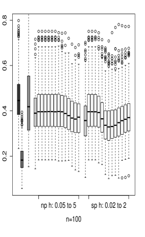
Refer to caption
Refer to caption
Refer to caption
Figure 1: Each boxplot is based on 500500500 estimates of |ฮฒ^โˆ’ฮฒ0|2superscript^๐›ฝsubscript๐›ฝ02|\widehat{\beta}-\beta_{0}|^{2} when q=4๐‘ž4q=4 and ฯƒ0โ€‹(x)=ฮฒ02Tโ€‹x|ฮฒ02|subscript๐œŽ0๐‘ฅsuperscriptsubscript๐›ฝ02๐‘‡๐‘ฅsubscript๐›ฝ02\sigma_{0}(x)=\frac{\beta_{02}^{T}x}{|\beta_{02}|}. The parametric, nonparametric (np) and semiparametric (sp) approaches are respectively based on (i), (ii) and (iii).
Refer to caption
Refer to caption
Refer to caption
Figure 2: Each boxplot is based on 500500500 estimates of |ฮฒ^โˆ’ฮฒ0|2superscript^๐›ฝsubscript๐›ฝ02|\widehat{\beta}-\beta_{0}|^{2} when q=16๐‘ž16q=16 and ฯƒ0โ€‹(x)=ฮฒ02Tโ€‹x|ฮฒ02|subscript๐œŽ0๐‘ฅsuperscriptsubscript๐›ฝ02๐‘‡๐‘ฅsubscript๐›ฝ02\sigma_{0}(x)=\frac{\beta_{02}^{T}x}{|\beta_{02}|}. The parametric, nonparametric (np) and semiparametric (sp) approaches are respectively based on (i), (ii) and (iii).
Refer to caption
Refer to caption
Refer to caption
Figure 3: Each boxplot is based on 500500500 estimates of |ฮฒ^โˆ’ฮฒ0|2superscript^๐›ฝsubscript๐›ฝ02|\widehat{\beta}-\beta_{0}|^{2} when q=4๐‘ž4q=4 and ฯƒ0โ€‹(x)=12+2โ‹…๐Ÿ™{ฮฒ02Tโ€‹x>0}subscript๐œŽ0๐‘ฅ12โ‹…2subscript1superscriptsubscript๐›ฝ02๐‘‡๐‘ฅ0\sigma_{0}(x)=\frac{1}{2}+2\cdot\mathds{1}_{\{\beta_{02}^{T}x>0\}}. The parametric, nonparametric (np) and semiparametric (sp) approaches are respectively based on (i), (ii) and (iii).
Refer to caption
Refer to caption
Refer to caption
Figure 4: Each boxplot is based on 500500500 estimates of |ฮฒ^โˆ’ฮฒ0|2superscript^๐›ฝsubscript๐›ฝ02|\widehat{\beta}-\beta_{0}|^{2} when q=16๐‘ž16q=16 and ฯƒ0โ€‹(x)=12+2โ‹…๐Ÿ™{ฮฒ02Tโ€‹x>0}subscript๐œŽ0๐‘ฅ12โ‹…2subscript1superscriptsubscript๐›ฝ02๐‘‡๐‘ฅ0\sigma_{0}(x)=\frac{1}{2}+2\cdot\mathds{1}_{\{\beta_{02}^{T}x>0\}}. The parametric, nonparametric (np) and semiparametric (sp) approaches are respectively based on (i), (ii) and (iii).

The figures 1 to 4 gives boxplots associated to the estimation error of each method, parametric (i), nonparametric (ii), and semiparamteric (iii), according to different values of n=50,100,500๐‘›50100500n=50,100,500, q=4,16๐‘ž416q=4,16 and ฯƒ0=ฯƒ01,ฯƒ02subscript๐œŽ0subscript๐œŽ01subscript๐œŽ02\sigma_{0}=\sigma_{01},\sigma_{02}. We also consider the first-step estimator ฮฒ^(0)superscript^๐›ฝ0\widehat{\beta}^{(0)} and a โ€œreference estimatorโ€ computed with the unknown optimal weights, i.e., ฮฒ^โ€‹(w0)^๐›ฝsubscript๐‘ค0\widehat{\beta}(w_{0}). In every case, the accuracy of each method lies between the first step estimator and the reference estimator. In agreement with Theorem 5 and 6, the gap between the reference estimator and the method (i), (ii), (iii) diminishes as n๐‘›n increases. Each method (i), (ii), (iii), performs differently showing that their equivalence occurs only at very large sample size.

Among the three methods under evaluation (i), (ii), (iii), the clear winner is the semiparametric method (with selection of the bandwidth by cross validation). The fact that it over-rules the nonparametric estimator was somewhat predictable, but the difference in accuracy with the parametric method is surprising. In every situation, the variance and the mean of the error associated to the semiparametric approach are smaller than the variance and the mean of the others. Moreover, the nonparametric method performs as well as the parametric method even in high-dimensional settings. In fact, both approaches are similarly affected by the increase of the dimension. Finally, one sees that the choice of the bandwidth by cross validation works well for both methods nonparametric and semiparametric. In all cases, the estimator with hcโ€‹vsubscriptโ„Ž๐‘๐‘ฃh_{cv} performs similarly to the estimator with the optimal hโ„Žh.

6 Appendix: concentration rates for kernel regression estimators

The result follows from the formulation of Talagrand inequality (Talagrand, 1994) given in Theorem 2.1 in Ginรฉ and Guillou (2002).

Lemma 7.

Let (Yiโˆˆโ„,Xiโˆˆโ„q,i=1,โ€ฆ,n)formulae-sequencesubscript๐‘Œ๐‘–โ„formulae-sequencesubscript๐‘‹๐‘–superscriptโ„๐‘ž๐‘–1โ€ฆ๐‘›(Y_{i}\in\mathbb{R},\ X_{i}\in\mathbb{R}^{q},\ i=1,\ldots,n) denote a sequence of random variables independent and identically distributed such that X1subscript๐‘‹1X_{1} has a bounded density f๐‘“f. Given K~:โ„qโ†ฆโ„:~๐พmaps-tosuperscriptโ„๐‘žโ„\widetilde{K}:\mathbb{R}^{q}\mapsto\mathbb{R} such that โˆซK~โ€‹(u)2โ€‹๐‘‘u<+โˆž~๐พsuperscript๐‘ข2differential-d๐‘ข\int\widetilde{K}(u)^{2}du<+\infty and ฮจฮจ\Psi a class of real functions defined on โ„q+1superscriptโ„๐‘ž1\mathbb{R}^{q+1}, if both classes ฮจฮจ\Psi and {K~โ€‹(xโˆ’โ‹…h),xโˆˆโ„q,h>0}\{\widetilde{K}\left(\frac{x-\cdot}{h}\right),\ x\in\mathbb{R}^{q},\ h>0\} are bounded measurable Vโ€‹C๐‘‰๐ถVC classes, it holds that

supฯˆโˆˆฮจ,xโˆˆ๐’ฌ|1nโ€‹โˆ‘i=1n{ฯˆโ€‹(Yi,Xi)โ€‹K~hโ€‹(xโˆ’Xi)โˆ’Eโ€‹[ฯˆโ€‹(Y1,X1)โ€‹K~hโ€‹(xโˆ’X1)]}|=OPโˆžโ€‹(|logโก(h)|nโ€‹hq).subscriptsupremumformulae-sequence๐œ“ฮจ๐‘ฅ๐’ฌ1๐‘›superscriptsubscript๐‘–1๐‘›๐œ“subscript๐‘Œ๐‘–subscript๐‘‹๐‘–subscript~๐พโ„Ž๐‘ฅsubscript๐‘‹๐‘–๐ธdelimited-[]๐œ“subscript๐‘Œ1subscript๐‘‹1subscript~๐พโ„Ž๐‘ฅsubscript๐‘‹1subscript๐‘‚subscript๐‘ƒโ„Ž๐‘›superscriptโ„Ž๐‘ž\displaystyle\sup_{\psi\in\Psi,\ x\in\mathcal{Q}}\left|\frac{1}{n}\sum_{i=1}^{n}\big{\{}\psi(Y_{i},X_{i})\widetilde{K}_{h}(x-X_{i})-E[\psi(Y_{1},X_{1})\widetilde{K}_{h}(x-X_{1})]\big{\}}\right|=O_{P_{\infty}}\left(\sqrt{\frac{|\log(h)|}{nh^{q}}}\right).
Proof.

The empirical process to consider is indexed by the product class ฮจโ€‹๐’ฆ~hฮจsubscript~๐’ฆโ„Ž\Psi\widetilde{\mathcal{K}}_{h}, where ๐’ฆ~h={K~โ€‹(xโˆ’โ‹…h),xโˆˆโ„q}\widetilde{\mathcal{K}}_{h}=\{\widetilde{K}(\frac{x-\cdot}{h}),\ x\in\mathbb{R}^{q}\} which is uniformly bounded Vโ€‹C๐‘‰๐ถVC since the product of two uniformly bounded Vโ€‹C๐‘‰๐ถVC classes remains uniformly bounded Vโ€‹C๐‘‰๐ถVC. The variance satisfies

var(ฯˆ(Y1,X1)K~(hโˆ’1(xโˆ’X1))\displaystyle\text{var}(\psi(Y_{1},X_{1})\widetilde{K}(h^{-1}(x-X_{1})) โ‰คEโ€‹ฯˆโ€‹(Y1,X1)2โ€‹K~โ€‹(hโˆ’1โ€‹(xโˆ’X1))2absent๐ธ๐œ“superscriptsubscript๐‘Œ1subscript๐‘‹12~๐พsuperscriptsuperscriptโ„Ž1๐‘ฅsubscript๐‘‹12\displaystyle\leq E\psi(Y_{1},X_{1})^{2}\widetilde{K}(h^{-1}(x-X_{1}))^{2}
โ‰คโ€–ฯˆโ€–โˆž2โ€‹โ€–fโ€–โˆžโ€‹hqโ€‹โˆซK~โ€‹(u)2โ€‹๐‘‘u,absentsuperscriptsubscriptnorm๐œ“2subscriptnorm๐‘“superscriptโ„Ž๐‘ž~๐พsuperscript๐‘ข2differential-d๐‘ข\displaystyle\leq\|\psi\|_{\infty}^{2}\|f\|_{\infty}h^{q}\int\widetilde{K}(u)^{2}du,

and a uniform bound is given by โ€–ฯˆโ€‹K~โ€–โˆžโ‰คsupฯˆโˆˆฮจโ€–ฯˆโ€–โˆžโ€‹โ€–K~โ€–โˆžsubscriptnorm๐œ“~๐พsubscriptsupremum๐œ“ฮจsubscriptnorm๐œ“subscriptnorm~๐พ\|\psi\widetilde{K}\|_{\infty}\leq\sup_{\psi\in\Psi}\|\psi\|_{\infty}\|\widetilde{K}\|_{\infty}. The application of Theorem 2.1 in Ginรฉ and Guillou (2002) gives the specified bound. โˆŽ

References

  • Andrews (1994) Andrews, D. W.ย K. (1994). Asymptotics for semiparametric econometric models via stochastic equicontinuity. Econometricaย 62(1), 43โ€“72.
  • Bates and White (1993) Bates, C.ย E. and H.ย White (1993). Determination of estimators with minimum asymptotic covariance matrices. Econometric Theoryย 9(04), 633โ€“648.
  • Carroll (1982) Carroll, R.ย J. (1982). Adapting for heteroscedasticity in linear models. Ann. Statist.ย 10(4), 1224โ€“1233.
  • Carroll and Ruppert (1982) Carroll, R.ย J. and D.ย Ruppert (1982). Robust estimation in heteroscedastic linear models. Ann. Statist.ย 10(2), 429โ€“441.
  • Carroll etย al. (1988) Carroll, R.ย J., C.-F.ย J. Wu, and D.ย Ruppert (1988). The effect of estimating weights in weighted least squares. J. Amer. Statist. Assoc.ย 83(404), 1045โ€“1054.
  • Chen etย al. (2003) Chen, X., O.ย Linton, and I.ย Vanย Keilegom (2003). Estimation of semiparametric models when the criterion function is not smooth. Econometricaย 71(5), 1591โ€“1608.
  • Ginรฉ and Guillou (2002) Ginรฉ, E. and A.ย Guillou (2002). Rates of strong uniform consistency for multivariate kernel density estimators. Ann. Inst. H. Poincarรฉ Probab. Statist.ย 38(6), 907โ€“921. En lโ€™honneur de J. Bretagnolle, D. Dacunha-Castelle, I. Ibragimov.
  • Huber (1967) Huber, P.ย J. (1967). The behavior of maximum likelihood estimates under nonstandard conditions. In Proc. Fifth Berkeley Sympos. Math. Statist. and Probability (Berkeley, Calif., 1965/66), Vol. I: Statistics, pp.ย  221โ€“233. Univ. California Press, Berkeley, Calif.
  • Kato (2009) Kato, K. (2009). Asymptotics for argmin processes: convexity arguments. J. Multivariate Anal.ย 100(8), 1816โ€“1829.
  • Kosorok (2008) Kosorok, M.ย R. (2008). Introduction to empirical processes and semiparametric inference. Springer Series in Statistics. New York: Springer.
  • Li (1991) Li, K.-C. (1991). Sliced inverse regression for dimension reduction. J. Amer. Statist. Assoc.ย 86(414), 316โ€“342.
  • Newey (1990) Newey, W.ย K. (1990). Efficient instrumental variables estimation of nonlinear models. Econometricaย 58(4), 809โ€“837.
  • Newey (1994) Newey, W.ย K. (1994). The asymptotic variance of semiparametric estimators. Econometricaย 62(6), 1349โ€“1382.
  • Newey and McFadden (1994) Newey, W.ย K. and D.ย McFadden (1994). Large sample estimation and hypothesis testing. In Handbook of econometrics, Vol.ย IV, Volumeย 2 of Handbooks in Econom., pp.ย  2111โ€“2245. Elsevier.
  • Nolan and Pollard (1987) Nolan, D. and D.ย Pollard (1987). U๐‘ˆU-processes: rates of convergence. Ann. Statist.ย 15(2), 780โ€“799.
  • Ojeda (2008) Ojeda, J. (2008). Hรถlder continuity properties of the local polynomial estimator. Pre-publicaciones del Seminario Matemรกticoโ€ Garcรญa de Galdeanoโ€ย 0(4), 1โ€“21.
  • Pollard (1985) Pollard, D. (1985). New ways to prove central limit theorems. Econometric Theoryย 1(03), 295โ€“313.
  • Portier and Delyon (2013) Portier, F. and B.ย Delyon (2013). Optimal transformation: A new approach for covering the central subspace. Journal of Multivariate Analysisย 115, 84โ€“107.
  • Robinson (1987) Robinson, P.ย M. (1987). Asymptotically efficient estimation in the presence of heteroskedasticity of unknown form. Econometricaย 55(4), 875โ€“891.
  • Talagrand (1994) Talagrand, M. (1994). Sharper bounds for Gaussian and empirical processes. Ann. Probab.ย 22(1), 28โ€“76.
  • vanย der Vaart (1995) vanย der Vaart, A.ย W. (1995). Efficiency of infinite-dimensional M๐‘€M-estimators. Statist. Neerlandicaย 49(1), 9โ€“30.
  • vanย der Vaart (1998) vanย der Vaart, A.ย W. (1998). Asymptotic statistics, Volumeย 3 of Cambridge Series in Statistical and Probabilistic Mathematics. Cambridge: Cambridge University Press.
  • vanย der Vaart and Wellner (1996) vanย der Vaart, A.ย W. and J.ย A. Wellner (1996). Weak convergence and empirical processes. Springer Series in Statistics. New York: Springer-Verlag. With applications to statistics.
  • vanย der Vaart and Wellner (2007) vanย der Vaart, A.ย W. and J.ย A. Wellner (2007). Empirical processes indexed by estimated functions. In Asymptotics: particles, processes and inverse problems, Volumeย 55 of IMS Lecture Notes Monogr. Ser., pp.ย  234โ€“252. Beachwood, OH: Inst. Math. Statist.