Dropping Convexity for Faster Semi-definite Optimization
Abstract
We study the minimization of a convex function over the set of positive semi-definite matrices, but when the problem is recast as , with and . We study the performance of gradient descent on —which we refer to as Factored Gradient Descent (Fgd)—under standard assumptions on the original function .
We provide a rule for selecting the step size and, with this choice, show that the local convergence rate of Fgd mirrors that of standard gradient descent on the original : i.e., after steps, the error is for smooth , and exponentially small in when is (restricted) strongly convex. In addition, we provide a procedure to initialize Fgd for (restricted) strongly convex objectives and when one only has access to via a first-order oracle; for several problem instances, such proper initialization leads to global convergence guarantees.
Fgd and similar procedures are widely used in practice for problems that can be posed as matrix factorization. To the best of our knowledge, this is the first paper to provide precise convergence rate guarantees for general convex functions under standard convex assumptions.
1 Introduction
Consider the following standard convex semi-definite optimization problem:
| (1) |
where is a convex and differentiable function, and denotes the convex set over positive semi-definite matrices in . Let be an optimum of (1) with . This problem can be remodeled as a non-convex problem, by writing where is an matrix. Specifically, define and111While is a non-convex function, we note that it is a very specific kind of non-convexity, arising “only” due to the recasting of an originally convex function. consider direct optimization of the transformed problem, i.e.,
| (2) |
Problems (1) and (2) will have the same optimum when . However, the recast problem is unconstrained and leads to computational gains in practice: e.g., iterative update schemes, like gradient descent, do not need to do eigen-decompositions to satisfy semi-definite constraints at every iteration.
In this paper, we also consider the case of , which often occurs in applications. The reasons of such a choice chould be three-fold: it might model better an underlying task (e.g., may have arisen from a relaxation of a rank constraint in the first place), it leads to computational gains, since smaller means fewer variables to maintain and optimize, it leads to statistical “gains”, as it might prevent over-fitting in machine learning or inference problems.
Such recasting of matrix optimization problems is empirically widely popular, especially as the size of problem instances increases. Some applications in modern machine learning includes matrix completion [21, 42, 49, 22], affine rank minimization [65, 41, 8], covariance / inverse covariance selection [38, 50], phase retrieval [64, 18, 77, 68], Euclidean distance matrix completion [56], finding the square root of a PSD matrix [40], and sparse PCA [26], just to name a few. Typically, one can solve (2) via simple, first-order methods on like gradient descent. Unfortunately, such procedures have no guarantees on convergence to the optima of the original , or on the rate thereof. Our goal in this paper is to provide such analytical guarantees, by using—simply and transparently—standard convexity properties of the original .
Overview of our results. In this paper, we prove that updating via gradient descent in (2) converges (fast) to optimal (or near-optimal) solutions. While there are some recent and very interesting works that consider using such non-convex parametrization [42, 64, 71, 82, 69, 81], their results only apply to specific examples. To the best of our knowledge, this is the first paper that solves the re-parametrized problem with attractive convergence rate guarantees for general convex functions and under common convex assumptions. Moreover, we achieve the above by assuming the first order oracle model: for any matrix , we can only obtain the value and the gradient .
To achieve the desiderata, we study how gradient descent over performs in solving (2). This leads to the factored gradient descent (Fgd) algorithm, which applies the simple update rule
| (3) |
We provide a set of sufficient conditions to guarantee convergence. We show that given a suitable initialization point, Fgd converges to a solution close to the optimal point in sublinear or linear rate, depending on the nature of .
Our contributions in this work can be summarized as follows:
-
New step size rule and Fgd. Our main algorithmic contribution is a special choice of the step size . Our analysis showcase that needs to depend not only on the convexity parameters of (as is the case in standard convex optimization) but also on the top singular value of the unknown optimum. Section 3 describes the precise step size rule, and also the intuition behind it. Of course, the optimum is not known a priori. As a solution in practice, we show that choosing based on a point that is constant relative distance from the optimum also provably works.
-
Convergence of Fgd under common convex assumptions. We consider two cases: when is just a -smooth convex function, and when satisfies also restricted strong convexity (RSC), i.e., satisfies strong-convexity-like conditions, but only over low rank matrices; see next section for definitions. Both cases are based on now-standard notions, common for the analysis of convex optimization algorithms. Given a good initial point, we show that, when is -smooth, Fgd converges sublinearly to an optimal point . For the case where has RSC, Fgd converges linearly to the unique , matching analogous result for classic gradient descent schemes, under smoothness and strong convexity assumptions.
Furthermore, for the case of smooth and strongly convex , our analysis extends to the case , where Fgd converges to a point close to the best rank- approximation of .222In this case, we require to be small enough, such that the rank-constrained optimum be close to the best rank- approximation of . This assumption naturally applies in applications, where e.g., is a superposition of a low rank latent matrix, plus a small perturbation term [43, 78]. In Section I, we show how this assumption can be dropped by using a different step size , where spectral norm computation of two matrices is required per iteration.
Both results hold when Fgd is initialized at a point with constant relative distance from optimum. Interestingly, the linear convergence rate factor depends not only on the convexity parameters of , but also on the spectral characteristics of the optimum; a phenomenon borne out in our experiments. Section 4 formally states these results.
-
Initialization: For specific problem settings, various initialization schemes are possible (see [42, 64, 23]). In this paper, we extend such results to the case where we only have access to via the first-order oracle: specifically, we initialize based on the gradient at zero, i.e., . We show that, for certain condition numbers of , this yields a constant relative error initialization (Section 5). Moreover, Section 5 lists alternative procedures that lead to good initialization points and comply with our theory.
Roadmap.
The rest of the paper is organized as follows. Section 2 contains basic notation and standard convex definitions. Section 3 presents the Fgd algorithm and the step size used, along with some intuition for its selection. Section 4 contains the convergence guarantees of Fgd; the main supporting lemmas and proofs of the main theorems are provided in Section 6. In Section 5, we discuss some initialization procedures that guarantee a “decent” starting point for Fgd. This paper concludes with discussion on related work (Section 7).
2 Preliminaries
Notation. For matrices , their inner product is . Also, denotes is a positive semi-definite (PSD) matrix, while the convex set of PSD matrices is denoted . We use and for the Frobenius and spectral norms of a matrix, respectively. Given a matrix , we use and to denote the smallest and largest strictly positive singular values of and define ; with a slight abuse of notation, we also use . denotes the rank- approximation of via its truncated singular value decomposition. Let denote the condition number of ; again, observe . denotes the basis of the column space of matrix . represents the stable rank of matrix . We use to denote the standard basis vector with 1 at the -th position and zeros elsewhere.
Without loss of generality, is a symmetric convex function, i.e., . Let denote the gradient matrix, i.e., its element is . For , the gradient of with respect to is , due to symmetry of . Finally, let be the optimum of over with factorization .
For any general symmetric matrix , let the matrix be its projection onto the set of PSD matrices. This can be done by finding all the strictly positive eigenvalues and corresponding eigenvectors and then forming .
In algorithmic descriptions, and denote the putative solution of current and next iteration, respectively. An important issue in optimizing over the space is the existence of non-unique possible factorizations for any feasible point . To see this, given factorization where , one can define an class of equivalent factorizations , where belongs to the set of rotational matrices. So we use a rotation invariant distance metric in the factored space that is equivalent to distance in the matrix space, which is defined below.
Definition 2.1.
Let matrices . Define:
is the set of orthonormal matrices , such that . The optimal satisfies where is the singular value decomposition of .
Assumptions. We will investigate the performance of non-convex gradient descent for functions that satisfy standard smoothness conditions only, as well as the case where further is (restricted) strongly convex. We state these standard definitions below.
Definition 2.2.
Let be convex and differentiable. Then, is -strongly convex if:
| (4) |
Definition 2.3.
Let be a convex differentiable function. Then, is -smooth if:
| (5) |
This further implies the following upper bound:
| (6) |
Given the above definitions, we define as the condition number of function .
Finally, in high dimensional settings, often loss function does not satisfy strong convexity globally, but only on a restricted set of directions; see [59, 2] and Section F for a more detailed discussion.
Definition 2.4.
A convex function is -restricted strongly convex if:
| (7) |
3 Factored gradient descent
We solve the non-convex problem (2) via Factored Gradient Descent (Fgd) with update rule333The true gradient of with respect to is . However, for simplicity and clarity of exposition, in our algorithm and its theoretical guarantees, we absorb the 2-factor in the step size .:
Fgd does this, but with two key innovations: a careful initialization and a special step size . The discussion on the initialization is deferred until Section 5.
Step size .
Even though is a convex function over , the fact that we operate with the non-convex parametrization means that we need to be careful about the step size ; e.g., our constant selection should be such that, when we are close to , we do not “overshoot” the optimum .
In this work, we pick the step size parameter, according to the following closed-form444Constant in the expression (8) appears due to our analysis, where we do not optimize over the constants. One can use another constant in order to be more aggressive; nevertheless, we observed that our setting works well in practice. :
| (8) |
Recall that, if we were just doing standard gradient descent on , we would choose a step size of , where is a uniform upper bound on the largest eigenvalue of the Hessian .
To motivate our step size selection, let us consider a simple setting where with ; i.e., is a vector. For clarity, denote it as . Let be a separable function with . Furthermore, define the function such that . It is easy to compute (see Lemma E.1):
where and, are the matricization, vectorization and diagonalization operations, respectively; for the last case, diag generates a diagonal matrix from the input, discarding its off-diagonal elements. We remind that and . Note also that is diagonal for separable .
Standard convex optimization suggests that should be chosen such that . The above suggest the following step size selection rule for -smooth :
In stark contrast with classic convex optimization where , the step size selection further depends on the spectral information of the current iterate and the gradient. Since computing per iteration could be computational inefficient, we use the spectral norm of and its gradient as surrogate, where is the initialization point555However, as we show in Section I, one could compute and per iteration in order to relax some of the requirements of our approach..
To clarify selection further, we next describe a toy example, in order to illustrate the necessity of such a scaling of the step size. Consider the following minimization problem.
where —and thus, , i.e., we are interested in rank-1 solutions—and is a given rank-2 matrix such that , for and orthonormal vectors. Observe that is a strongly convex function with rank-1 minimizer ; let . It is easy to verify that , , and , where .
Consider the case where is the current estimate. Then, the gradient of at is evaluated as:
Hence, according to the update rule , the next iterate satisfies:
Observe that coefficients of both in include and quantities.
The quality of clearly depends on how is chosen. In the case , such step size can result in divergence“overshooting”, as and can be arbitrarily large (independent of ). Therefore, it could be the case that .
In contrast, consider the step size666For illustration purposes, we consider a step size that depends on the unknown ; in practice, our step size selection is a surrogate of this choice and our results automatically carry over, with appropriate scaling. . Then, with appropriate scaling , we observe that lessens the effect of and terms in and terms, that lead to overshooting for the case . This most possibly result in .
Computational complexity.
The per iteration complexity of Fgd is dominated by the gradient computation. This computation is required in any first order algorithm and the complexity of this operation depends on the function . Apart from , the additional computation required in Fgd is matrix-matrix additions and multiplications, with time complexity upper bounded by , where denotes the number of non zeros in the gradient at the current point.777It could also occur that gradient is low-rank, or low-rank + sparse, depending on the problem at hand; it could also happen that the structure of leads to “cheap” matrix-vector calculations, when applied to vectors. Here, we state a more generic –and maybe pessimistic– scenario where is unstructured. Hence, the per iteration complexity of Fgd is much lower than traditional convex methods like projected gradient descent [60] or classic interior point methods [62, 63], as they often require a full eigenvalue decomposition per step.
Note that, for , Fgd and projected gradient descent have same per iteration complexity of . However, Fgd performs only a single matrix-matrix multiplication operation, which is much “cheaper” than a SVD calculation. Moreover, matrix multiplication is an easier-to-parallelize operation, as opposed to eigen decomposition operation which is inherently sequential. We notice this behavior in practice; see Sections F, G and H for applications in matrix sensing and quantum state tomography.
4 Local convergence of Fgd
In this section, we present our main theoretical results on the performance of Fgd. We present convergence rates for the settings where is a -smooth convex function, and is a -smooth and -restricted strongly convex function. These assumptions are now standard in convex optimization. Note that, since the factorization makes the problem non-convex, it is hard to guarantee convergence of gradient descent schemes in general, without any additional assumptions.
We now state the main assumptions required by Fgd for convergence:
Fgd Assumptions
-
•
Initialization: We assume that Fgd is initialized with a “good” starting point that has constant relative error to .888If , then one can drop the subscript. For completeness and in order to accommodate the approximate rank- case, described below, we will keep the subscript in our discussion. In particular, we assume
-
for (Smooth )
-
for (Strongly convex ),
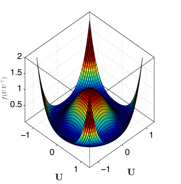
for the smooth and restricted strongly convex setting, respectively. This assumption helps in avoiding saddle points, introduced by the parametrization999To illustrate this consider the following example, Now it is easy to see that and is a stationary point of the function considered . We need the initial error to be further smaller than by a factor of condition number of ..
In many applications, an initial point with this type of guarantees is easy to obtain, often with just one eigenvalue decomposition; we refer the reader to the works [42, 64, 23, 82, 71] for specific initialization procedures for different problem settings. See also Section 5 for a more detailed discussion. Note that the problem is still non-trivial after the initialization, as this only gives a constant error approximation.
-
-
•
Approximate rank- optimum: In many learning applications, such as localization [43] and multilabel learning [78], the true emerges as the superposition of a low rank latent matrix plus a small perturbation term, such that is small. While, in practice, it might be the case —due to the presence of noise—often we are more interested in revealing the latent low-rank part. As already mentioned, we might as well set for computational or statistical reasons. In all these cases, further assumptions w.r.t. the quality of approximation have to be made. In particular, let be the optimum of (1) and is -smooth and -strongly convex. In our analysis, we assume:
-
(Strongly convex ),
This assumption intuitively requires the noise magnitude to be smaller than the optimum and constrains the rank constrained optimum to be closer to .101010Note that the assumption can be dropped by using a different step size (see Theorem I.4 in Section I). However, this requires two additional spectral norm computations per iteration.
-
We note that, in the results presented below, we have not attempted to optimize over the constants appearing in the assumptions and any intermediate steps of our analysis. Finding such tight constants could strengthen our arguments for fast convergence; however, it does not change our claims for sublinear or linear convergence rates. Moreover, we consider the case ; we believe the analysis can be extended to the setting and leave it for future work.111111Experimental results on synthetic matrix sensing settings have shown that, if we overshoot , i.e., , Fgd still performs well, finding an -accurate solution with linear rate.
4.1 convergence rate for smooth
Next, we state our first main result under smoothness condition, as in Definition 2.3. In particular, we prove that Fgd makes progress per iteration with sublinear rate. Here, we assume only the case where ; for consistency reasons, we denote . Key lemmas and their proofs for this case are provided in Section C.
Theorem 4.1 (Convergence performance for smooth ).
Let denote an optimum of -smooth over the PSD cone. Let . Then, under assumption , after iterations, the FGD algorithm finds solution such that
| (9) |
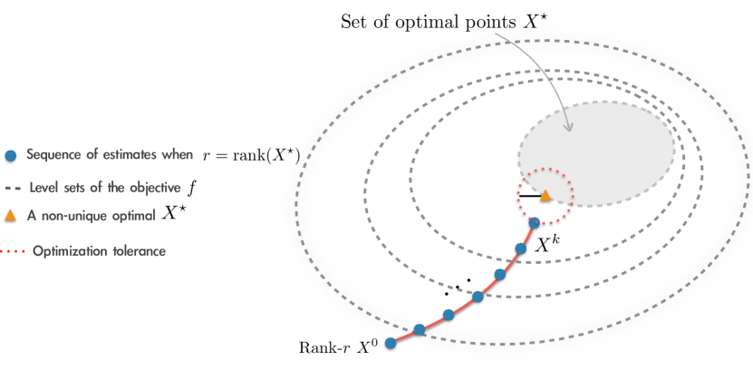
The theorem states that provided we choose the step size , based on a starting point that has constant relative distance to , and we start from such a point, gradient descent on will converge sublinearly to a point . In other words, Theorem 4.1 shows that Fgd computes a sequence of estimates in the -factor space such that the function values decrease with rate, towards a global minimum of function. Recall that, even in the standard convex setting, classic gradient descent schemes over achieve the same convergence rate for smooth convex functions [60]. Hence, Fgd matches the rate of convex gradient descent, under the assumptions of Theorem 4.1. The above are abstractly illustrated in Figure 1.
4.2 Linear convergence rate under strong convexity assumption
Here, we show that, with the additional assumption that satisfies the -restricted strong convexity over , Fgd achieves linear convergence rate. The proof is provided in Section B.
Theorem 4.2 (Convergence rate for restricted strongly convex ).
Let the current iterate be and . Assume and let the step size be . Then under assumptions , the new estimate satisfies
| (10) |
where and . Furthermore, satisfies
The theorem states that provided we choose the step size based on a point that has constant relative distance to , and we start from such a point, gradient descent on will converge linearly to a neighborhood of . The above theorem immediately implies linear convergence rate for the setting where is standard strongly convex, with parameter . This follows by observing that standard strong convexity implies restricted strong convexity for all values of rank .
Last, we present results for the special case where ; in this case, Fgd finds an optimal point with linear rate, within the equivalent class of orthonormal matrices in .
Corollary 4.3 (Exact recovery of ).
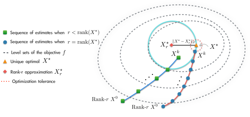
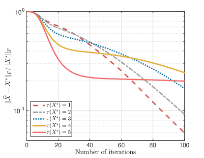
Further, for we recover the exact case of semi-definite optimization. In plain words, the above corollary suggests that, given an accuracy parameter , Fgd requires iterations in order to achieve ; recall the analogous result for classic gradient schemes for -smooth and strongly convex functions , where similar rates can be achieved in space [60]. The above are abstractly illustrated in Figure 2.
Remark 1.
By the results above, one can easily observe that the convergence rate factor , in contrast to standard convex gradient descent results, depends both on the condition number of and , in addition to . This dependence is a result of the step size selection, which is different from standard step sizes, i.e., for standard gradient descent schemes. We also refer the reader to Section E for some discussion.
As a ramification of the above, notice that depends only on the condition number of and not that of . This suggests that, in settings where the optimum has bad condition number (and thus leads to slower convergence), it is indeed beneficial to restrict to be a matrix and only search for a rank- approximation of the optimal solution, which leads to faster convergence rate in practice; see Figure 8 in our experimental findings at the end of Section F.3.
Remark 2.
In the setting where the optimum is 0, directly applying the above theorems requires an initialization that is exactly at the optimum 0. On the contrary, this is actually an easy setting and the Fgd converges from any initial point to the optimum.
5 Initialization
In the previous section, we show that gradient descent over achieves sublinearlinear convergence, once the iterates are closer to . Since the overall problem is non-convex, intuition suggests that we need to start from a “decent” initial point, in order to get provable convergence to .
One way to satisfy this condition for general convex is to use one of the standard convex algorithms and obtain within constant error to (or ); then, switch to Fgd to get the high precision solution. See [71] for a specific implementation of this idea on matrix sensing. Such initialization procedure comes with the following guarantees; the proof can be found in Section D:
Lemma 5.1.
Let be a -smooth and -restricted strongly convex function over PSD matrices and let be the minimum of with . Let be the projected gradient descent update. Then, implies,
Next, we present a generic initialization scheme for general smooth and strongly convex . We use only the first-order oracle: we only have access to—at most—gradient information of . Our initialization comes with theoretical guarantees w.r.t. distance from optimum. Nevertheless, in order to show small relative distance in the form of , one requires certain condition numbers of and further assumptions on the spectrum of optimal solution and rank . However, empirical findings in Section F.3 show that our initialization performs well in practice.
Let . Since the initial point should be in the PSD cone, we further consider the projection . By strong convexity and smoothness of , one can observe that the point is a good initialization point, within some radius from the vicinity of ; i.e.,
| (11) |
see also Theorem 5.2. Thus, a scaling of by could serve as a decent initialization. In many recent works [42, 64, 19, 82, 23] this initialization has been used for specific applications.121212To see this, consider the case of least-squares objective , where denote the set of observations and, is a properly designed sensing mechanism, depending on the problem at hand. For example, in the affine rank minimization case [82, 23], represents the linear system mechanism where . Under this setting, computing the gradient at zero point, we have: , where is the adjoint operator of . Then, it is obvious that the operation is very similar to the spectral methods, proposed for initialization in the references above. Here, we note that the point can be used as initialization point for generic smooth and strongly convex .
The smoothness parameter is not always easy to compute exactly; in such cases, one can use the surrogate . Finally, our initial point is a rank- matrix such that .
We now present guarantees for the initialization discussed. The proof is provided in Section D.2.
Theorem 5.2 (Initialization).
Let be a -smooth and -strongly convex function, with condition number , and let be its minimum over PSD matrices. Let be defined as:
| (12) |
and is its rank- approximation. Let for some . Then, , where and .
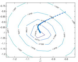
While the above result guarantees a good initialization for only small values of , in many applications [42, 64, 23], this is indeed the case and has constant relative error to the optimum.
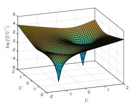
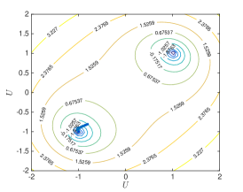
To understand this result, notice that in the extreme case, when is the loss function , which has condition number and , indeed is the optimum. More generally as the condition number increases, the optimum moves away from and the above theorem characterizes this error as a function of condition number of the function. See also Figure 3.
Now for the setting when the optimum is exactly rank- we get the following result.
Corollary 5.3 (Initialization, exact).
Let be rank- for some . Then, under the conditions of Theorem 5.2, we get
Finally, for the setting when the function satisfies -restricted strong convexity, the above corollary still holds as the optimum is a rank- matrix.
6 Convergence proofs for the Fgd algorithm
In this section, we first present the key techniques required for analyzing the convergence of Fgd. Later, we present proofs for both Theorems 4.1 and 4.2. Throughout the proofs we use the following notation. is the optimum of problem (1) and is the rank- approximation; for the just smooth case, , as we consider only the rank- case and . Let and .
A key property that assists classic gradient descent to converge to the optimum is the fact that for a smooth convex function ; in the case of strongly convex , the inner product is further lower bounded by (see Theorem 2.2.7 of [60]). Classical proofs mainly use such lower bounds to show convergence (see Theorems 2.1.13 and 2.2.8 of [60]).
We follow broadly similar steps in order to show convergence of Fgd. In particular,
- •
- •
6.1 Rudiments of our analysis
Next, we present the main descent lemma that is used for both sublinear and linear convergence rate guarantees of Fgd.
Lemma 6.1 (Descent lemma).
For being a -smooth and -strongly convex function and, under assumptions and , the following inequality holds true:
Further, when is just -smooth convex function and, under the assumptions and , we have:
Proof.
First, we rewrite the inner product as shown below.
| (13) |
which follows by adding and subtracting .
-
•
Strongly convex setting. For this case, the next 3 steps apply.
Step I: Bounding . The first term in the above expression can be lower bounded using smoothness and strong convexity of and, involves a construction of a feasible point . We construct such a feasible point by modifying the current update to one with bigger step size .
Lemma 6.2.
Let be a -smooth and -restricted strongly convex function with optimum point . Moreover, let be the best rank- approximation of . Let . Then,
where , by Lemma A.5.
Proof of this lemma is provided in Section B.1.
Step II: Bounding . The second term in equation (13) can actually be negative. Hence, we lower bound it using our initialization assumptions. Intuitively, the second term is smaller than the first one as it scales as , while the first term scales as .
Lemma 6.3.
Let be -smooth and -restricted strongly convex. Then, under assumptions and , the following bound holds true:
Proof of this lemma can be found in Section B.2.
-
•
Smooth setting. For this case, the next 3 steps apply.
Step I: Bounding . Similar to the strongly convex case, one can obtain a lower bound on , according to the following Lemma:
Lemma 6.4.
Let be a -smooth convex function with optimum point . Then, under the assumption that , the following holds:
The proof of this lemma can be found in Appendix C.
Step II: Bounding . Here, we follow a different path in providing a lower bound for . The following lemma provides such a lower bound.
Lemma 6.5.
Let and define . Let . Then, for , where , and being a -smooth convex function, the following lower bound holds:
The proof of this lemma can be found in Appendix C.
Step III: Combining the bounds in equation (13). For a detailed description, see Section C and Lemma C.4.
∎
6.2 Proof of linear convergence (Theorem 4.2)
The proof of this theorem involves showing that the potential function is decreasing per iteration (up to approximation error ), using the descent Lemma 6.1. Using the algorithm’s update rule, we obtain
| (14) |
which follows by adding and subtracting and then expanding the squared term.
Step I: Bounding term in (14). By Lemma 6.1, we can bound the last term on the right hand side as:
Furthermore, we can substitute in the first term to obtain .
Step II: Combining bounds into (14). Combining the above two equations (14) becomes:
where is due to removing the negative part from the right hand side, is due to by Lemma A.5, follows from substituting . This proves the first part of the theorem.
Step III: satisfies the initial condition. Now we will prove the second part. By the above equation, we have:
follows from substituting the assumptions on and and the last inequality is due to the term in the parenthesis being less than one.
6.3 Proof of sublinear convergence (Theorem 4.1)
Here, we show convergence of Fgd when is only a -smooth convex function. At iterate , we assume ; in the opposite case, the bound follows trivially. Recall the updates of Fgd over the -space satisfy
It is easy to verify that , where . Notice that for step size , using Lemma A.5 we get,
| (15) |
Our proof proceeds using the smoothness condition on , at point . In particular,
where follows from symmetry of , and
| (16) |
and is due to (15) and the fact that (see Lemma A.5). Hence,
| (17) |
To bound the term on the right hand side of (17), we use standard convexity as follows:
| (18) |
where is due to and for orthonormal matrix , is by , is due to Cauchy-Schwarz inequality and Lemma C.1 and, is due to norm ordering .
From (18), we obtain to the following bound:
| (19) |
Define and . Moreover, by Lemma C.5, we know that for all iterations of FGD; thus, we have for every update . Using the above definitions and substituting (19) in (17), we obtain the following recursion:
which can be further transformed as:
since from equation (17). Since each and correspond to previous and new estimate in FGD per iteration, we can sum up the above inequalities over iterations to obtain
here, and . After simple transformations, we finally obtain131313One can further obtain a bound on the right hand side that depends on . By Lemma A.5, we know . Thus, the current proof leads to the bound: :
This finishes the proof.
7 Related work
Convex approaches. A significant volume of work has focused on solving the classic Semi-Definite Programming (SDP) formulation, where the objective (as well as any additional convex constraints) is assumed to be linear. There, interior point methods (IPMs) constitute a popular choice for small- and moderate-sized problems; see [46, 3]. For a comprehensive treatment of this subject, see the excellent survey in [57].
Large scale SDPs pointed research towards first-order approaches, which are more computationally appealing. For linear , we note among others the work of [76], a provably convergent alternating direction augmented Lagrangian algorithm, and that of Helmberg and Rendl [36], where they develop an efficient first-order spectral bundle method for SDPs with the constant trace property; see also [35] for extensions on this line of work. In both cases, no convergence rate guarantees are provided; see also [57]. For completeness, we also mention the work of [14, 31, 58, 70] on second-order methods, that take advantage of data sparsity in order to handle large SDPs in a more efficient way. However, it turns out that the amount of computations required per iteration is comparable to that of log-barrier IPMs [57].
Standard SDPs have also found application in the field of combinatorial optimization; there, in most cases, even a rough approximation to the discrete problem, via SDP, is sufficiently accurate and computationally affordable, than exhaustive combinatorial algorithms. Goemans and Williamson [32] were the first to propose the use of SDPs in approximating graph Max Cut, where a near-optimum solution can be found in polynomial time. [48] propose an alternative approach for solving Max Cut and Graph Coloring instances, where SDPs are transformed into eigenvalue problems. Then, power method iterations lead to -approximate solutions; however, the resulting running-time dependence on is worse, compared to standard IPMs. Arora, Hazan and Kale in [4] derive an algorithm to approximate SDPs, as a hybrid of the Multiplicative Weights Update method and of ideas originating from an ellipsoid variant [73], improving upon existing algorithms for graph partitioning, computational biology and metric embedding problems.141414The algorithm in [4] shows significant computational gains over standard IPMs per iteration, due to requiring only a power method calculation per iteration (versus a Cholesky factorization per iteration, in the latter case). However, the polynomial dependence on the accuracy parameter is worse, compared to IPMs. Improvements upon this matter can be found in [5] where a primal-dual Multiplicative Weights Update scheme is proposed.
Extending to non-linear convex cases, [62, 63] have shown how IPMs can be generalized to solve instances of (1), via the notion of self-concordance; see also [53, 27] for a more recent line of work. Within the class of first-order methods, approaches for nonlinear convex include, among others, projected and proximal gradient descent methods [60, 27, 44], (smoothed) dual ascent methods [61], as well as Frank-Wolfe algorithm variants [39]. Note that all these schemes, often require heavy calculations, such as eigenvalue decompositions, to compute the updates (often, to remain within the feasible set).
Burer & Monteiro factorization and related work. Burer and Monteiro [15, 16] popularized the idea of solving classic SDPs by representing the solution as a product of two factor matrices. The main idea in such representation is to remove the positive semi-definite constraint by directly embedding it into the objective. While the problem becomes non-convex, Burer and Monteiro propose a method-of-multiplier type of algorithm which iteratively updates the factors in an alternating fashion. For linear objective , they establish convergence guarantees to the optimum but do not provide convergence rates.
For generic smooth convex functions, Hazan in [34] proposes SparseApproxSDP algorithm,151515Sparsity here corresponds to low-rankness of the solution, as in the Cholesky factorization representation. Moreover, inspired by Quantum State Tomography applications [1], SparseApproxSDP can also handle constant trace constraints, in addition to PSD ones. a generalization of the Frank-Wolfe algorithm for the vector case [25], where putative solutions are refined by rank-1 approximations of the gradient. At the -th iteration, SparseApproxSDP is guaranteed to compute a -approximate solution, with rank at most , i.e., achieves a sublinear convergence rate. However, depending on , SparseApproxSDP is not guaranteed to return a low rank solution unlike Fgd. Application of these ideas in machine learning tasks can be found in [67]. Based on SparseApproxSDP algorithm, [51] further introduces “de-bias” steps in order to optimize parameters in SparseApproxSDP and do local refinements of putative solutions via L-BFGS steps. Nevertheless, the resulting convergence rate is still sublinear.161616For running time comparisons with Fgd see Sections G and H.
Specialized algorithms – for objectives beyond the linear case – that utilize such factorization include matrix completion /sensing solvers [42, 69, 82, 71], non-negative matrix factorization schemes [52], phase retrieval methods [64, 19] and sparse PCA algorithms [51]. Most of these results guarantee linear convergence for various algorithms on the factored space starting from a “good” initialization. They also present a simple spectral method to compute such an initialization. For the matrix completion /sensing setting, [66] have shown that stochastic gradient descent achieves global convergence at a sublinear rate. Note that these results only apply to quadratic loss objectives and not to generic convex functions .171717We recently became aware of the extension of the work [71] for the non-square case . [40] consider the problem of computing the matrix square-root of a PSD matrix via gradient descent on the factored space: in this case, the objective boils down to minimizing the standard squared Euclidean norm distance between two matrices. Surprisingly, the authors show that, given an initial point that is well-conditioned, the proposed scheme is guaranteed to find an -accurate solution with linear convergence rate.
[23] propose a first-order optimization framework for the problem (1), where the same parametrization technique is used to efficiently accommodate the PSD constraint.181818In this work, the authors further assume orthogonality of columns in . Moreover, the proposed algorithmic solution can accommodate extra constraints on .191919Though, additional constraints should satisfy the -faithfulness property: a constraint set on , say , is faithful if for each , that is within some bounded radius from optimal point, we are guaranteed that the closest (in the Euclidean sense) rotation of lies within . The set of assumptions listed in [23] include—apart from -faithfulness—local descent, local Lipschitz and local smoothness conditions in the factored space. E.g., the local descent condition can be established if is locally strongly convex and at an optimum point vanishes. They also require bounded gradients as their step size doesn’t account for the modified curvature of . 202020One can define non-trivially conditions on the original space; we defer the reader to [23] These conditions are less standard than the global assumptions of the current work and one needs to validate that they are satisfied for each problem, separately. [23] presents some applications where these conditions are indeed satisfied. Their results are of the same flavor with ours: under such proper assumptions, one can prove local convergence with or rate and for instances that even fail to be locally convex.
Finally, for completeness, we also mention optimization over the Grassmannian manifold that admits tailored solvers [28]; see [47, 10, 11, 80, 72] for applications in matrix completion and references therein. [45] presents a second-order method for (1), based on manifold optimization over the set of all equivalence class . The proposed algorithm can additionally accommodate constraints and enjoys monotonic decrease of the objective function (in contrast to [15, 16]), featuring quadratic local convergence. In practice, the per iteration complexity is dominated by the extraction of the eigenvector, corresponding to the smallest eigenvalue, of a matrix—and only when the current estimate of rank satisfies some conditions.
Table 1 summarizes the comparison of the most relevant work to ours, for the case of matrix factorization techniques.
| Reference | Conv. rate | Initialization | Output rank | |||
| [34] | (Smooth ) | |||||
| [51] | (Smooth ) | |||||
| [23] | (Local Asm.) | Application dependent | ||||
| [23] | (Local Asm.) | Application dependent | ||||
| This work | (Smooth ) | SVD top- | ||||
| This work | (Smooth, RSC ) | SVD top- |
8 Conclusion
In this paper, we focus on how to efficiently minimize a convex function over the positive semi-definite cone. Inspired by the seminal work [15, 16], we drop convexity by factorizing the optimization variable and show that factored gradient descent with a non-trivial step size selection results in linear convergence when is smooth and (restricted) strongly convex, even though the problem is now non-convex. In the case where is only smooth, only sublinear rate is guaranteed. In addition, we present initialization schemes that use only first order information and guarantee to find a starting point with small relative distance from optimum.
There are many possible directions for future work, extending the idea of using non-convex formulation for semi-definite optimization. Showing convergence under weaker initialization condition or without any initialization requirement is definitely of great interest. Another interesting direction is to improve the convergence rates presented in this work, by using acceleration techniques and thus, extend ideas used in the case of convex gradient descent [60]. Finally, it would be valuable to see how the techniques presented in this paper can be generalized to other standard algorithms like stochastic gradient descent and coordinate descent.
References
- [1] Scott Aaronson. The learnability of quantum states. In Proceedings of the Royal Society of London A: Mathematical, Physical and Engineering Sciences, volume 463, pages 3089–3114. The Royal Society, 2007.
- [2] Alekh Agarwal, Sahand Negahban, and Martin J Wainwright. Fast global convergence rates of gradient methods for high-dimensional statistical recovery. In Advances in Neural Information Processing Systems, pages 37–45, 2010.
- [3] Farid Alizadeh. Interior point methods in semidefinite programming with applications to combinatorial optimization. SIAM Journal on Optimization, 5(1):13–51, 1995.
- [4] Sanjeev Arora, Elad Hazan, and Satyen Kale. Fast algorithms for approximate semidefinite programming using the multiplicative weights update method. In Foundations of Computer Science, 2005. FOCS 2005. 46th Annual IEEE Symposium on, pages 339–348. IEEE, 2005.
- [5] Sanjeev Arora and Satyen Kale. A combinatorial, primal-dual approach to semidefinite programs. In Proceedings of the thirty-ninth annual ACM symposium on Theory of computing, pages 227–236. ACM, 2007.
- [6] Megasthenis Asteris, Dimitris Papailiopoulos, Anastasios Kyrillidis, and Alexandros G Dimakis. Sparse PCA via bipartite matchings. arXiv preprint arXiv:1508.00625, 2015.
- [7] S. Becker, E. Candès, and M. Grant. Templates for convex cone problems with applications to sparse signal recovery. Mathematical Programming Computation, 3(3):165–218, 2011.
- [8] Stephen Becker, Volkan Cevher, and Anastasios Kyrillidis. Randomized low-memory singular value projection. In 10th International Conference on Sampling Theory and Applications (Sampta), 2013.
- [9] Rajendra Bhatia. Perturbation bounds for matrix eigenvalues, volume 53. SIAM, 1987.
- [10] Nicolas Boumal. Optimization and estimation on manifolds. PhD thesis, UC Louvain, Belgium, 2014.
- [11] Nicolas Boumal. A riemannian low-rank method for optimization over semidefinite matrices with block-diagonal constraints. arXiv preprint arXiv:1506.00575, 2015.
- [12] Stephen Boyd and Lieven Vandenberghe. Convex optimization. Cambridge university press, 2004.
- [13] Sébastien Bubeck. Theory of convex optimization for machine learning. arXiv preprint arXiv:1405.4980, 2014.
- [14] Samuel Burer. Semidefinite programming in the space of partial positive semidefinite matrices. SIAM Journal on Optimization, 14(1):139–172, 2003.
- [15] Samuel Burer and Renato DC Monteiro. A nonlinear programming algorithm for solving semidefinite programs via low-rank factorization. Mathematical Programming, 95(2):329–357, 2003.
- [16] Samuel Burer and Renato DC Monteiro. Local minima and convergence in low-rank semidefinite programming. Mathematical Programming, 103(3):427–444, 2005.
- [17] J. Cai, E. Candès, and Z. Shen. A singular value thresholding algorithm for matrix completion. SIAM Journal on Optimization, 20(4):1956–1982, 2010.
- [18] Emmanuel J Candes, Yonina C Eldar, Thomas Strohmer, and Vladislav Voroninski. Phase retrieval via matrix completion. SIAM Review, 57(2):225–251, 2015.
- [19] Emmanuel J Candes, Xiaodong Li, and Mahdi Soltanolkotabi. Phase retrieval via wirtinger flow: Theory and algorithms. Information Theory, IEEE Transactions on, 61(4):1985–2007, 2015.
- [20] Emmanuel J Candes and Yaniv Plan. Tight oracle inequalities for low-rank matrix recovery from a minimal number of noisy random measurements. Information Theory, IEEE Transactions on, 57(4):2342–2359, 2011.
- [21] Emmanuel J Candès and Benjamin Recht. Exact matrix completion via convex optimization. Foundations of Computational mathematics, 9(6):717–772, 2009.
- [22] Yudong Chen, Srinadh Bhojanapalli, Sujay Sanghavi, and Rachel Ward. Coherent matrix completion. In Proceedings of The 31st International Conference on Machine Learning, pages 674–682, 2014.
- [23] Yudong Chen and Martin J Wainwright. Fast low-rank estimation by projected gradient descent: General statistical and algorithmic guarantees. arXiv preprint arXiv:1509.03025, 2015.
- [24] Yuxin Chen and Sujay Sanghavi. A general framework for high-dimensional estimation in the presence of incoherence. In Communication, Control, and Computing (Allerton), 2010 48th Annual Allerton Conference on, pages 1570–1576. IEEE, 2010.
- [25] Kenneth L Clarkson. Coresets, sparse greedy approximation, and the Frank-Wolfe algorithm. ACM Transactions on Algorithms (TALG), 6(4):63, 2010.
- [26] Alexandre d’Aspremont, Laurent El Ghaoui, Michael I Jordan, and Gert RG Lanckriet. A direct formulation for sparse PCA using semidefinite programming. SIAM review, 49(3):434–448, 2007.
- [27] Quoc Tran Dinh, Anastasios Kyrillidis, and Volkan Cevher. Composite self-concordant minimization. Journal of Machine Learning Research, 16:371–416, 2015.
- [28] Alan Edelman, Tomás A Arias, and Steven T Smith. The geometry of algorithms with orthogonality constraints. SIAM journal on Matrix Analysis and Applications, 20(2):303–353, 1998.
- [29] M. Fazel. Matrix rank minimization with applications. PhD thesis, PhD thesis, Stanford University, 2002.
- [30] S. Flammia, D. Gross, Y.-K. Liu, and J. Eisert. Quantum tomography via compressed sensing: Error bounds, sample complexity and efficient estimators. New Journal of Physics, 14(9):095022, 2012.
- [31] Mituhiro Fukuda, Masakazu Kojima, Kazuo Murota, and Kazuhide Nakata. Exploiting sparsity in semidefinite programming via matrix completion I: General framework. SIAM Journal on Optimization, 11(3):647–674, 2001.
- [32] Michel X Goemans and David P Williamson. Improved approximation algorithms for maximum cut and satisfiability problems using semidefinite programming. Journal of the ACM (JACM), 42(6):1115–1145, 1995.
- [33] David Gross, Yi-Kai Liu, Steven T Flammia, Stephen Becker, and Jens Eisert. Quantum state tomography via compressed sensing. Physical review letters, 105(15):150401, 2010.
- [34] Elad Hazan. Sparse approximate solutions to semidefinite programs. In LATIN 2008: Theoretical Informatics, pages 306–316. Springer, 2008.
- [35] Christoph Helmberg, Michael L Overton, and Franz Rendl. The spectral bundle method with second-order information. Optimization Methods and Software, 29(4):855–876, 2014.
- [36] Christoph Helmberg and Franz Rendl. A spectral bundle method for semidefinite programming. SIAM Journal on Optimization, 10(3):673–696, 2000.
- [37] Roger A Horn and Charles R Johnson. Topics in matrix analysis. Cambridge University Presss, Cambridge, 37:39, 1991.
- [38] Cho-Jui Hsieh, Inderjit S Dhillon, Pradeep K Ravikumar, and Mátyás A Sustik. Sparse inverse covariance matrix estimation using quadratic approximation. In Advances in Neural Information Processing Systems, pages 2330–2338, 2011.
- [39] Martin Jaggi. Convex optimization without projection steps. arXiv preprint arXiv:1108.1170, 2011.
- [40] Prateek Jain, Chi Jin, Sham M Kakade, and Praneeth Netrapalli. Computing matrix squareroot via non convex local search. arXiv preprint arXiv:1507.05854, 2015.
- [41] Prateek Jain, Raghu Meka, and Inderjit S Dhillon. Guaranteed rank minimization via singular value projection. In Advances in Neural Information Processing Systems, pages 937–945, 2010.
- [42] Prateek Jain, Praneeth Netrapalli, and Sujay Sanghavi. Low-rank matrix completion using alternating minimization. In Proceedings of the 45th annual ACM symposium on Symposium on theory of computing, pages 665–674. ACM, 2013.
- [43] Adel Javanmard and Andrea Montanari. Localization from incomplete noisy distance measurements. Foundations of Computational Mathematics, 13(3):297–345, 2013.
- [44] Kaifeng Jiang, Defeng Sun, and Kim-Chuan Toh. An inexact accelerated proximal gradient method for large scale linearly constrained convex SDP. SIAM Journal on Optimization, 22(3):1042–1064, 2012.
- [45] Michel Journée, Francis Bach, P-A Absil, and Rodolphe Sepulchre. Low-rank optimization on the cone of positive semidefinite matrices. SIAM Journal on Optimization, 20(5):2327–2351, 2010.
- [46] Narendra Karmarkar. A new polynomial-time algorithm for linear programming. In Proceedings of the sixteenth annual ACM symposium on Theory of computing, pages 302–311. ACM, 1984.
- [47] Raghunandan H Keshavan, Andrea Montanari, and Sewoong Oh. Matrix completion from a few entries. Information Theory, IEEE Transactions on, 56(6):2980–2998, 2010.
- [48] Philip Klein and Hsueh-I Lu. Efficient approximation algorithms for semidefinite programs arising from MAX CUT and COLORING. In Proceedings of the twenty-eighth annual ACM symposium on Theory of computing, pages 338–347. ACM, 1996.
- [49] Anastasios Kyrillidis and Volkan Cevher. Matrix recipes for hard thresholding methods. Journal of mathematical imaging and vision, 48(2):235–265, 2014.
- [50] Anastasios Kyrillidis, Rabeeh Karimi, Quoc Tran Dinh, and Volkan Cevher. Scalable sparse covariance estimation via self-concordance. In Twenty-Eighth AAAI Conference on Artificial Intelligence, 2014.
- [51] Soeren Laue. A hybrid algorithm for convex semidefinite optimization. In Proceedings of the 29th International Conference on Machine Learning (ICML-12), pages 177–184, 2012.
- [52] Daniel D Lee and H Sebastian Seung. Algorithms for non-negative matrix factorization. In Advances in neural information processing systems, pages 556–562, 2001.
- [53] Jason Lee, Yuekai Sun, and Michael Saunders. Proximal newton-type methods for convex optimization. In Advances in Neural Information Processing Systems, pages 836–844, 2012.
- [54] Yi-Kai Liu. Universal low-rank matrix recovery from Pauli measurements. In Advances in Neural Information Processing Systems, pages 1638–1646, 2011.
- [55] Leon Mirsky. A trace inequality of John von Neumann. Monatshefte für Mathematik, 79(4):303–306, 1975.
- [56] Bamdev Mishra, Gilles Meyer, and Rodolphe Sepulchre. Low-rank optimization for distance matrix completion. In Decision and control and European control conference (CDC-ECC), 2011 50th IEEE conference on, pages 4455–4460. IEEE, 2011.
- [57] Renato DC Monteiro. First-and second-order methods for semidefinite programming. Mathematical Programming, 97(1-2):209–244, 2003.
- [58] Kazuhide Nakata, Katsuki Fujisawa, Mituhiro Fukuda, Masakazu Kojima, and Kazuo Murota. Exploiting sparsity in semidefinite programming via matrix completion II: Implementation and numerical results. Mathematical Programming, 95(2):303–327, 2003.
- [59] Sahand Negahban and Martin J Wainwright. Restricted strong convexity and weighted matrix completion: Optimal bounds with noise. The Journal of Machine Learning Research, 13(1):1665–1697, 2012.
- [60] Yurii Nesterov. Introductory lectures on convex optimization, volume 87. Springer Science & Business Media, 2004.
- [61] Yurii Nesterov. Smoothing technique and its applications in semidefinite optimization. Mathematical Programming, 110(2):245–259, 2007.
- [62] Yurii Nesterov and Arkadi Nemirovski. A general approach to polynomial-time algorithms design for convex programming. Report, Central Economical and Mathematical Institute, USSR Academy of Sciences, Moscow, 1988.
- [63] Yurii Nesterov and Arkadi Nemirovski. Self-concordant functions and polynomial-time methods in convex programming. USSR Academy of Sciences, Central Economic & Mathematic Institute, 1989.
- [64] Praneeth Netrapalli, Prateek Jain, and Sujay Sanghavi. Phase retrieval using alternating minimization. In Advances in Neural Information Processing Systems, pages 2796–2804, 2013.
- [65] Benjamin Recht, Maryam Fazel, and Pablo A Parrilo. Guaranteed minimum-rank solutions of linear matrix equations via nuclear norm minimization. SIAM review, 52(3):471–501, 2010.
- [66] Christopher D Sa, Christopher Re, and Kunle Olukotun. Global convergence of stochastic gradient descent for some non-convex matrix problems. In Proceedings of the 32nd International Conference on Machine Learning (ICML-15), pages 2332–2341, 2015.
- [67] Shai Shalev-shwartz, Alon Gonen, and Ohad Shamir. Large-scale convex minimization with a low-rank constraint. In Proceedings of the 28th International Conference on Machine Learning (ICML-11), pages 329–336, 2011.
- [68] Ju Sun, Qing Qu, and John Wright. A geometric analysis of phase retrieval. arXiv preprint arXiv:1602.06664, 2016.
- [69] Ruoyu Sun and Zhi-Quan Luo. Guaranteed matrix completion via non-convex factorization. arXiv preprint arXiv:1411.8003, 2014.
- [70] Kim-Chuan Toh. Solving large scale semidefinite programs via an iterative solver on the augmented systems. SIAM Journal on Optimization, 14(3):670–698, 2004.
- [71] Stephen Tu, Ross Boczar, Mahdi Soltanolkotabi, and Benjamin Recht. Low-rank solutions of linear matrix equations via Procrustes flow. arXiv preprint arXiv:1507.03566, 2015.
- [72] Andre Uschmajew and Bart Vandereycken. Greedy rank updates combined with riemannian descent methods for low-rank optimization. In 12th International Conference on Sampling Theory and Applications (Sampta), 2015.
- [73] Pravin M Vaidya. A new algorithm for minimizing convex functions over convex sets. In Foundations of Computer Science, 1989., 30th Annual Symposium on, pages 338–343. IEEE, 1989.
- [74] Vincent Q Vu, Jing Lei, et al. Minimax sparse principal subspace estimation in high dimensions. The Annals of Statistics, 41(6):2905–2947, 2013.
- [75] Andrew E Waters, Aswin C Sankaranarayanan, and Richard Baraniuk. Sparcs: Recovering low-rank and sparse matrices from compressive measurements. In Advances in neural information processing systems, pages 1089–1097, 2011.
- [76] Zaiwen Wen, Donald Goldfarb, and Wotao Yin. Alternating direction augmented Lagrangian methods for semidefinite programming. Mathematical Programming Computation, 2(3-4):203–230, 2010.
- [77] Chris D White, Sujay Sanghavi, and Rachel Ward. The local convexity of solving systems of quadratic equations. arXiv preprint arXiv:1506.07868, 2015.
- [78] Hsiang-Fu Yu, Prateek Jain, Purushottam Kar, and Inderjit Dhillon. Large-scale multi-label learning with missing labels. In Proceedings of The 31st International Conference on Machine Learning, pages 593–601, 2014.
- [79] A. Yurtsever, Q. Tran-Dinh, and V. Cevher. A universal primal-dual convex optimization framework. In Advances in Neural Information Processing Systems 28, pages 3132–3140. 2015.
- [80] Dejiao Zhang and Laura Balzano. Global convergence of a grassmannian gradient descent algorithm for subspace estimation. arXiv preprint arXiv:1506.07405, 2015.
- [81] Tuo Zhao, Zhaoran Wang, and Han Liu. A nonconvex optimization framework for low rank matrix estimation. In Advances in Neural Information Processing Systems, pages 559–567, 2015.
- [82] Qinqing Zheng and John Lafferty. A convergent gradient descent algorithm for rank minimization and semidefinite programming from random linear measurements. arXiv preprint arXiv:1506.06081, 2015.
Appendix A Supporting lemmata
Lemma A.1 (Hoffman, Wielandt [9]).
Let and be two PSD matrices. Also let be full rank. Then,
| (20) |
The following lemma shows that Dist, in the factor space, upper bounds the Frobenius norm distance in the matrix space.
Lemma A.2.
Let and be two rank- PSD matrices. Let , for some rotation matrix and constant . Then,
Proof.
By substituting and in , we have:
where is due to the orthogonality , is due to the triangle inequality, the Cauchy-Schwarz inequality and the fact that spectral norm is invariant w.r.t. orthogonal transformations and, is due to the following sequence of inequalities, based on the hypothesis of the lemma:
and thus . The final inequality follows from the hypothesis of the lemma. ∎
The following lemma connects the spectrum of to under the initialization assumptions.
Lemma A.3.
Let and be matrices such that , for . Withal, define . Then, the following bounds hold true:
Moreover, by definition of for some matrix, we also observe:
Proof.
Using the norm ordering and the Weyl’s inequality for perturbation of singular values (Theorem 3.3.16 [37]) we get,
Then, the first two inequalities of the lemma follow by using triangle inequality and the above bound. For the last two inequalities, it is easy to derive bounds on condition numbers by combining the first two inequalities. Viz.,
while the last bound can be easily derived since . ∎
The following lemma shows that Dist, in the factor space, lower bounds the Frobenius norm distance in the matrix space.
Lemma A.4.
Let and be two rank- PSD matrices. Let , for . Then,
Proof.
This proof largely follows the arguments for Lemma 5.4 in [71], from which we know that
| (21) |
Hence, , for the given value of . ∎
The following lemma shows equivalence between various step sizes used in the proofs.
Lemma A.5.
Let and be two rank- PSD matrices such that , where . Define the following step sizes:
-
,
-
, and
-
.
Then, holds. Moreover, assuming , the following inequalities hold:
Proof.
By the assumptions of this lemma and based on Lemma A.3, we have, ; similarly . Hence, we can combine these two set of inequalities to obtain bounds between and , as follows:
To prove the desiderata, we show the relationship between the gradient terms , and . In particular, for the case , we have:
where follows from the triangle inequality, is due to the smoothness assumption, is due to the triangle inequality, follows by applying Lemma A.2 on the first two terms on the right hand side and, is due to the fact and by substituting . Last inequality follows from . Hence, using the above bounds in step size selection, we get
where is based also on the bound .
Similarly we show the bound . First observe that,
Combining the above bound with gives, . Similarly we can show the other bounds. ∎
Appendix B Main lemmas for the restricted strong convex case
In this section, we present proofs for the main lemmas used in the proof of Theorem 4.2, in Section 6.
B.1 Proof of Lemma 6.2
Here, we prove the existence of a non-trivial lower bound for . Our proof differs from the standard convex gradient descent proof (see [60]), as we need to analyze updates without any projections. Our proof technique constructs a pseudo-iterate to obtain a bigger lower bound than the error term in Lemma 6.3. Here, the nature of the step size plays a key role in achieving the bound.
Let us abuse our notation and define and . Observe that we use the surrogate step size , where according to Lemma A.5 satisfies . By smoothness of , we get:
| (22) |
where follows from optimality of and since is a feasible point for problem (1). Further, note that is a PSD feasible point. By smoothness of , we also get
| (23) |
where is due to KKT conditions [12]: since is orthogonal to , it is also orthogonal to the bottom eigenvectors of . Viz., . Finally, since , by the -restricted strong convexity of , we get,
| (24) |
Combining equations (22), (23), and (24), we obtain:
| (25) |
It is easy to verify that , where . Notice that, for step size , we have
Substituting the above in (25), we obtain:
where follows from symmetry of and , and follows from
Finally, follows by observing that . Thus, we achieve the desiderata:
This completes the proof.
B.2 Proof of Lemma 6.3
We lower bound as follows:
| (26) |
Note that follows from the fact and follows from , for PSD matrix (Von Neumann’s trace inequality [55]). For the transformation in , we use that fact that the column space of , , is a subset of , as is a linear combination of and .
To bound the first term in equation (26), we observe:
| (27) | |||
At this point, we desire to introduce strong convexity parameter and condition number in our bound. In particular, to bound term , we observe that or . This results into bounding as follows:
Combining the above inequalities, we obtain:
| (28) | ||||
| (29) |
where follows from , is due to Lemma A.3 and bounding by the hypothesis of the lemma, is due to by Lemma A.3 and due to the facts and . Finally, follows from substituting and using Lemma A.3.
B.3 Proof of Lemma 6.1
Recall . First we rewrite the inner product as shown below.
| (32) |
which follows by adding and subtracting .
Appendix C Main lemmas for the smooth case
In this section, we present the main lemmas, used in the proof of Theorem 4.1 in Section 6. First, we present a lemma bounding the error term , that appears in eq. (18).
Lemma C.1.
Let be -smooth and ; also, define . Then, for and , the following bound holds true:
Proof.
By the Von Neumann’s trace inequality for PSD matrices, we know that , for PSD matrix. In our context, we then have:
| (33) |
where, is because can be decomposed into the column span of and , and the orthogonality of the rotational matrix . In sequence, we further bound the term as follows:
where is due to triangle inequality on , is due to generalized Cauchy-Schwarz inequality; we denote as the projection matrix on the column span of matrix, is due to triangle inequality and the fact that the column span of can be decomposed into the column span of and , by construction of , is due to
Finally, is due to the facts:
and
by Lemma A.3. Thus:
| (34) |
and, combining with (33), we get
The last inequality follows from . This completes the proof. ∎
The following lemma lower bounds the term ; this result is used later in the proof of Lemma C.4.
Lemma C.2.
Let and define . Let , where is the optimum of the problem (1). Then, for , where , and being a -smooth convex function, the following lower bound holds:
Proof.
Let the QR factorization of the matrix be , where is a orthonormal matrix and is a invertible matrix (since is assumed to be rank-). Further, let where denotes the pseudo-inverse of matrix . It is obvious that .
Given the above, let us re-define some quantities w.r.t. , as follows
Moreover, it is straightforward to justify that:
Then, from the above, the two quantities and are connected as follows:
which is equal to . Then, the following sequence of (in)equalities holds true:
| (35) |
where, follows by substituting , according to the discussion above, follows from symmetry of , follows from the Von Neumann trace inequality , for a PSD matrix ; next, we show that , and , is due to successive application of the Cauchy-Schwarz inequality, is due to and , follows from the the following fact:
where, follows from a variant of Weyl’s inequality, is due to , follows from the assumption that . The above lead to the inequality:
In the above inequalities (35), we used the fact that symmetric version of A is a PSD matrix, where is a PSD matrix, i.e., given a vector , . To show this, let be a function from . Hence, . Now, consider restricted to the level set . Note that, since is convex, this set is convex and further belongs to this set from the hypothesis of the lemma. Also , for in this set from the optimality of . Let be the minimizer of over this set. Then, by convexity of ,
Further, since , is orthogonal to . Hence, . Combining this with the above inequality gives, . This completes the proof. ∎
We next present a lemma for lower bounding the term . This result is used in the following Lemma C.4, where we bound the term .
Lemma C.3.
Let be a -smooth convex function with optimum point . Then, under the assumption that , the following holds:
Proof.
The proof follows much like the proof of the Lemma for strong convex case (Lemma 6.2), except for the arguments used to bound equation (22). For completeness, we here highlight the differences; in particular, we again have by smoothness of :
where we consider the same notation with Lemma 6.2. By the assumptions of the Lemma, we have and, thus, the above translates into:
hence eliminating the need for equation (23). Combining the above and assuming just smoothness (i.e., the restricted strong convexity parameter is ), we obtain a simpler version of eq. (25):
| (36) |
Then, the result easily follows by the same steps in Lemma 6.2. ∎
Next, we state an important result, relating the gradient step in the factored space to the direction to the optimum . The result borrows the outcome of Lemmas C.1-C.3.
Lemma C.4.
Let and define . Assume and , where . For being a -smooth convex function, the following descent condition holds for the -space:
Proof.
Expanding the term , we obtain the equivalent characterization:
| (37) |
which follows by the definition of and adding and subtracting term. By Lemma C.3, we can bound the first term on the right hand side as:
| (38) |
Observe that . By Lemma C.2, we can lower bound the last term on the right hand side of (37) as:
| (39) |
Combining (38) and (39) in (37), we get:
where follows from in Lemma A.5. This completes the proof. ∎
We conclude this section with a lemma that proves that the distance is non-increasing per iteration of Fgd. This lemma is used in the proof of sublinear convergence of Fgd (Theorem 4.1), in Section 6.
Lemma C.5.
Let and be the current and next estimate of Fgd. Assume is a -smooth convex function such that . Moreover, define and , where . Then, the following inequality holds:
This further implies for any estimate of Fgd.
Proof.
Appendix D Initialization proofs
D.1 Proof of Lemma 5.1
The proof borrows results from standard projected gradient descent. In particular, we know from Theorem 3.6 in [13] that, for consecutive estimates and optimal point , projected gradient descent satisfies:
By taking square root of the above inequality, we further have:
| (42) |
since , for all values of .
Given the above, the following (in)equalities hold true:
where is due to the lower bound on triangle inequality and is due to (42). Under the assumptions of the lemma, if , the above inequality translates into:
By construction, both and are PSD matrices; moreover, can be a matrix with . Hence,
using Weyl’s inequalities. Thus, Define and . Further, by Lemma 5.4 of [71], we have:
The above lead to:
Recall that ; then, by Lemma A.3, there is constant such that . Combining all the above, we conclude that there is constant such that:
D.2 Proof of Theorem 5.2
Recall . Here, we remind that is the projection operator onto the PSD cone and is the projection operator onto the negative semi-definite cone.
To bound we will bound each individual term in its squared expansion
From the smoothness of , we get the following:
where follows from non-expansiveness of projection operator and follows from the fact that is PSD and hence . Finally, observe that . The above combined imply:
where we used the fact that and . Hence .
Using the strong convexity of around , we observe
where the last inequality follows from first order optimality of , and 0 is a feasible point for problem (1). Similarly, using strong convexity of around , we have
Combining the above two inequalities we get, . Moreover:
since is PSD. Thus, and
| (43) |
where we used the fact that . Given the above inequalities, we can now prove the following:
Now we know that Now, by triangle inequality . By and Weyl’s inequality for perturbation of singular values (Theorem 3.3.16 [37]) we get,
By the assumptions of the theorem, we have . Therefore,
Now again using triangle inequality and substituting we get . Finally combining this with Lemma A.4 gives the result.
Appendix E Dependence on condition number in linear convergence rate
It is known that the convergence rate of classic gradient descent schemes depends only on the condition number of the function . However, in the case of Fgd, we notice that convergence rate also depends on condition number , as well as .
To elaborate more on this dependence, let us recall the update rule of Fgd, as presented in Section 3. In particular, one can observe that the gradient direction has an extra factor , multiplying , as compared to the standard gradient descent on . One way to reveal how this extra factor affects the condition number of the Hessian of , we consider the special case of separable functions; see the definition of separable functions in the next lemma. Next, we show that the condition number of the Hessian – for this special case – has indeed a dependence on both and , a scaling similar to the one appearing in the convergence rate of Fgd.
Lemma E.1 (Dependence of Hessian on and ).
Let be a smooth, twice differentiable function over the PSD cone. Further, assume is a separable function over the matrix entries, such that , where , and let ’s be -smooth and -strongly convex functions, . Finally, let be rank- and let denote the Hessian of w.r.t. the factor and up to rotations, for some rotation matrix . Then,
for constant . Further, for any unit vector such that columns of are orthogonal to , i.e., , we further have:
for some constant .
Proof.
By the definition of gradient, we know that ; for simplicity, we assume be symmetric. Since is symmetric, with and . By the definition of Hessian, the entries of are given by:
In particular, for we observe the following cases:
while, for we further have:
Consider now the case where gradient and Hessian information is calculated at the optimal point . Based on the above, the Hessian of w.r.t turns out to be a sum of three PSD matrices, as follows:
where
-
, where is a diagonal matrix with diagonal elements and is a matrix with repeated times on the diagonal. It is easy to see that
Similarly, we have
-
is a matrix, with . Again, it is easy to verify that . Now for perpendicular to , notice that , since the columns of are concatenation of scaled columns of .
-
is a diagonal block-matrix, with blocks repeated times. It is again easy to see that , since is a block diagonal matrix. Moreover, by KKT optimality condition , and thus, .
Combining the above results and observing that all the three matrices are PSD, we conclude that . Regarding the lower bound on , we observe the following: due to factorization and for optimum, we know that also is optimum, where gradient . This further indicates that the hessian of is zero along directions corresponding to columns of , and thus along these directions; see figure 4 (right panel) for an example. However, for any other directions orthogonal to , we have , for some constant . This completes the proof.
∎
To show this dependence in practice, we present some simulation results in Figure 4. We observe that the convergence rate does indeed depend on .
Appendix F Test case I: Matrix sensing problem
In this section, we briefly describe and compare algorithms designed specifically for the matrix sensing problem, using the variable parametrization . To accommodate the PSD constraint, we consider a variation of the matrix sensing problem where one desires to find that minimizes212121This problem is a special case of affine rank minimization problem [65], where no PSD constraints are present.:
| (44) |
W.l.o.g., we assume for some rank- . Here, is the linear sensing mechanism, such that the -th entry of is given by , for sub-Gaussian independent measurement matrices.
[42] is one of the first works to propose a provable and efficient algorithm for (44), operating in the -factor space, while [66] solves (44) in the stochastic setting; see also [82, 71, 23]. To guarantee convergence, most of these algorithms rely on restricted isometry assumptions; see Definition F.1 below.
To compare the above algorithms with Fgd, Subsection F.1 further describes the notion of restricted strong convexity and its connection with the RIP. Then, Subsection F.2 provides explicit comparison results of the aforementioned algorithms, with respect to the convergence rate factor , as well as initialization conditions assumed, for each case.
F.1 Restricted isometry property and restricted strong convexity
To shed some light on the notion of restricted strong convexity and how it relates to the RIP, consider the matrix sensing problem, as described above. According to (44), we consider the quadratic loss function:
Since the Hessian of is given by , restricted strong convexity suggests that [59]:
for a restricted set of directions , where is a small constant. This bound implies that the quadratic loss function, as defined above, is strongly convex in such a restricted set of directions .222222One can similarly define the notion of restricted smoothness condition, where is upper bounded by .
A similar but stricter notion is that of restricted isometry property for low rank matrices [20, 54]:
Definition F.1 (Restricted Isometry Property (RIP)).
A linear map satisfies the -RIP with constant , if
is satisfied for all matrices such that .
The correspondence of restricted strong convexity with the RIP is obvious: both lower bound the quantity , where is drawn from a restricted set. It turns out that linear maps that satisfy the RIP for low rank matrices, also satisfy the restricted strong convexity; see Theorem 2 in [24].
By assuming RIP in (44), the condition number of depends on the RIP constants of the linear map ; in particular, one can show that , since the eigenvalues of lie between and , when restricted to low-rank matrices. For sufficiently small and dimension sufficiently large, , which, with high probability, is the case for drawn from a sub-Gaussian distribution.
F.2 Comparison
Given the above discussion, the following hold true for Fgd, under RIP settings:
-
In the noiseless case, and thus, . Combined with the above discussion, this leads to convergence rate factor
in Fgd.
-
In the noisy case, where is an additive noise term; for this case, we further assume that is bounded. Then,
Table 2 summarizes convergence rate factors and initialization conditions of state-of-the-art approaches for the noiseless case.
| Reference | ||||
|---|---|---|---|---|
| [42] | ||||
| [71] | ||||
| [82] | ||||
| [23] | ||||
| This work |
F.3 Empirical results
We start our discussion on empirical findings with respect to the convergence rate of the algorithm, how the step size and initialization affects its efficiency and some comparison plots with an efficient first-order projected gradient solver. We note that the experiments presented below are performed as a proof of concept and are not complete in the set of algorithms we could compare with.
Linear convergence rate and step size selection:
To show the convergence rate of the factored gradient descent in practice, we solve affine rank minimization problems instances with synthetic data. In particular, the ground truth is synthesized as a rank- matrix as , where . In sequence, we sub-sample by observing entries, according to:
| (45) |
We use permuted and sub-sampled noiselets for the linear operator ; for more information, see [75]. contains the linear measurements of through in vectorized form. We consider the noiseless case, for ease of exposition. Under this setting, we solve (2) with . We use as a stopping criterion the condition where .
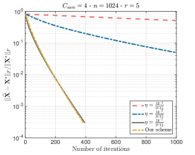
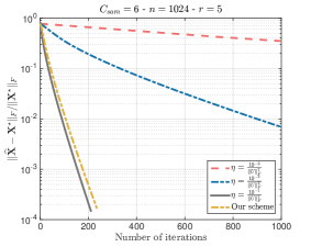
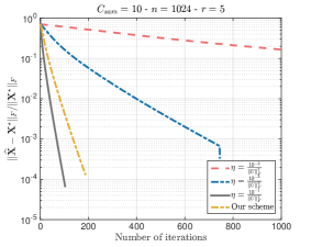
Figure 5 show the linear convergence of our approach as well as the efficiency of our step selection, as compared to other arbitrary constant step size selections. All instances use our initialization point. It is worth mentioning that the performance of our step size can be inferior to specific constant step size selections; however, finding such a good constant step size usually requires trial-and-error rounds and do not come with convergence guarantees. Moreover, we note that one can perform line search procedures to find the “best” step size per iteration; although, for more complicated instances, such step size selection might not be computationally desirable, even infeasible.
Impact of avoiding low-rank projections on the PSD cone:
In this experiment, we compare factored gradient descent with a variant of the Singular Value Projection (SVP) algorithm [41, 8]232323SVP is a non-convex, first-order, projected gradient descent scheme for low rank recovery from linear measurements.. For the purpose of this experiment, the SVP variant further projects on the PSD cone, along with the low rank projection. Its main difference is that it does not operate on the factor space but requires projection over the (low-rank) positive semi-definite cone per iteration. In the discussion below, we refer to this variant as SVP (SDP).
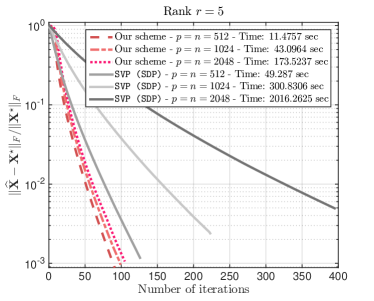
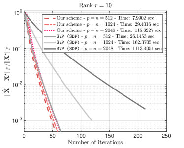
| Model | Time (sec) | ||||||
|---|---|---|---|---|---|---|---|
| SVP (SDP) | Our scheme | SVP (SDP) | Our scheme | ||||
| 1.1339e-03 | 8.4793e-04 | 36.9652 | 11.4757 | ||||
| 4.6552e-04 | 4.4954e-04 | 19.6089 | 7.9902 | ||||
| 1.6541e-04 | 2.0571e-04 | 10.6052 | 6.4149 | ||||
| 2.4224e-03 | 9.9180e-04 | 225.6230 | 43.0964 | ||||
| 1.0203e-03 | 4.5103e-04 | 121.7779 | 29.4016 | ||||
| 4.1149e-04 | 2.3442e-04 | 67.6272 | 22.9616 | ||||
| 4.8500e-03 | 1.0093e-03 | 1512.1969 | 173.5237 | ||||
| 2.0836e-03 | 4.6735e-04 | 835.0538 | 115.6227 | ||||
| 9.4893e-04 | 2.6417e-04 | 458.8766 | 88.1960 | ||||
We perform two experiments. In the first experiment, we compare factored gradient descent with SVP (SDP), as designed in [41]; i.e., while we use our initialization point for both schemes, step size selections are different. Figure 6 shows some convergence rate results: clearly our step size selection performs better in practice, in terms of the total number of iterations required for convergence.
In the second experiment, we would like to highlight the time bottleneck introduced by the projection operations: for this aim, we use the same initialization points and step sizes for both the algorithms under comparison. Thus, the only difference lies in the SVD computations of SVP (SDP) to retain a PSD low rank estimate per iteration. Table 3 presents reconstruction error and execution time results. It is obvious that projecting on the low-rank PSD code per iteration constitutes a computational bottleneck per iteration, which slows down (w.r.t. total time required) the convergence of SVP (SDP).
Initialization.
Here, we evaluate the importance of our initialization point selection:
| (46) |
To do so, we consider the following settings: we compare random initializations against the rule (46), both for constant step size selections and our step size selection. In all cases, we work with the factored parametrization.
Figure 7 shows the results. Left panel presents results for constant step size selections where and right panel uses our step size selection; again, note that the selection of the constant step size is after many trial-and-errors for best step size selection, based on the specific configuration. Both figures compare the performance of factored gradient descent when a random initialization point is selected and, our initialization is performed, according to (46). All curves depict median reconstruction errors over 20 Monte Carlo iterations. For all cases, the number of measurements is fixed to for and rank .
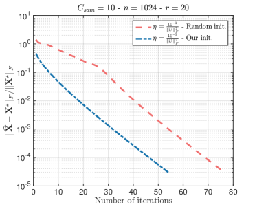
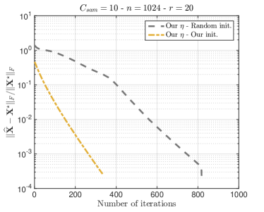
Dependence of on .
Here, we highlight the dependence of on the convergence rate of factored gradient descent. Consider the following matrix sensing toy example: let for and assume . We desire to compute a (at most) rank- approximation of by minimizing the simple least squares loss function:
| (47) | ||||||
| subject to |
For this example, let us consider and design according to the following three scenarios: we fix and vary . This leads to condition numbers for these three cases as: , and, . The convergence behavior is shown in Figure 8(Left panel). It is obvious that factored gradient descent suffers – w.r.t. convergence rate – as the condition number get worse; especially, for the case where , factored gradient descent reaches a plateau after the 80-th iteration, where the steps towards solution become smaller. As the condition number improves, factored gradient descent enjoys faster convergence to the optimum, which shows the dependence of the algorithm on also in practice.
As a second setting, we fix , thereby computing a rank- approximation. As Figure 8(Right panel) illustrates, for all values of , factored gradient descent performs similarly, enjoying fast convergence towards the optimum . Thus, while the condition number of original varies to a large degree for , the convergence rate factor only depends on , for . This leads to similar convergence behavior for all three scenarios described above.
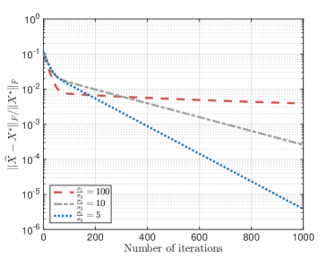
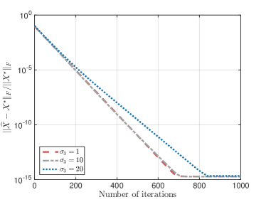
Appendix G Test case II: Quantum State Tomography
As a second example, we consider the quantum state tomography (QST) problem. QST can be described as follows:
| (48) | ||||||
| subject to |
In this problem, we look for a density matrix of a -bit quantum system from a set of QST measurements that satisfy . Here, and could be modeled as zero-mean Gaussian. The operators are typically the tensor product of the Pauli matrices [54]. The density matrix is a priori known to be Hermitian, positive semi-definite matrix that satisfies and is normalized as [33]; here, . Our task is to recover .
One can easily transform (48) into the following re-parameterized formulation:
| (49) | ||||||
| subject to |
It is apparent that this problem formulation is not included in the cases Fgd naturally solve, due to the Frobenius norm constraint on the factor . However, as a heuristic, one can alter Fgd to include such projection: per iteration, each putative solution can be trivially projected onto the Frobenious norm ball ; let us call this heuristic projFGD. We compare such algorithm with state-of-the-art scheme for QST to show the merits of our approach. The analysis of such constraint cases is an interesting and important extension of this paper and is left for future work.
State-of-the-art approaches.
One of the first provable algorithmic solutions for the QST problem was through convexification [29, 65, 21]: this includes nuclear norm minimization approaches [33] (using e.g., [7]), as well as proximal variants [30] (using e.g., [17]). Recently, [79] presented a universal primal-dual convex framework, which includes the QST problem as application and outperforms the above approaches, both in terms of recovery performance and execution time.
From a non-convex perspective, apart from Hazan’s algorithm [34] – see Related work, [8] propose Randomized Singular Value Projection (RSVP), a projected gradient descent algorithm for (48), which merges gradient calculations with truncated SVDs via randomized approximations for computational efficiency.
Experiments.
Figure 9 (two-leftmost plots) illustrates the iteration and timing complexities of each algorithm under comparison, for a pure state density recovery setting (). Here, which corresponds to a dimensional problem; moreover, we assume and thus the number of measurements are . For initialization, we use the proposed initialization for all algorithms. It is apparent that Fgd converges faster to a vicinity of , as compared to the rest of the algorithms; observe also the sublinear rate of SparseApproxSDP in the inner plots, as reported in [34].
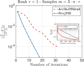
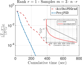
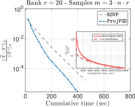
Appendix H Test case III: PSD problems with high-rank solutions
As a final example, we consider problems of the form:
where is the minimizer of the above problem and . In this particular case and assuming we are interested in finding high-ranked , we can reparameterized the above problem as follows:
Observe that is a square matrix. Under this setting, Fgd performs the recursion:
Due to the matrix-matrix multiplication, the per-iteration time complexity of Fgd is , which is comparable to a SVD calculation of a matrix. In this experiment, we study the performance of Fgd in such high-rank cases and compare it with state-of-the-art approaches for PSD constrained problems.
| Algorithm | Total time (sec) | Time per iter. (sec - median) | ||||
|---|---|---|---|---|---|---|
| Setting: , , . | ||||||
| RSVP | 4.9579e-04 | 1262.3719 | 2.1644 | |||
| SparseApproxSDP | 3.3329e-01 | 895.9605 | 2.1380e-01 | |||
| FGD | 1.6763e-04 | 57.8495 | 2.1961e-01 | |||
| Setting: , , . | ||||||
| RSVP | 4.9537e-04 | 8412.6981 | 14.6811 | |||
| SparseApproxSDP | 3.3526e-01 | 26962.0379 | 8.7761e-01 | |||
| FGD | 1.6673e-04 | 272.8102 | 1.0040e+00 | |||
| Setting: , , . | ||||||
| RSVP | 2.4254e-04 | 1945.6714 | 5.9763 | |||
| SparseApproxSDP | 9.6725e-02 | 3506.8147 | 8.6440e-01 | |||
| FGD | 3.8917e-05 | 68.5689 | 9.2567e-01 | |||
For the purpose of this experiment, we only consider first-order solvers; i.e., second order methods such as interior point methods are excluded as, in high dimensions, it is prohibitively expensive the hessian of . To this end, the algorithms to compare include: standard projected gradient descent approach [49] and Frank-Wolfe type of algorithms, such as the one in [34]. We note that this experiment can be seen as a proof of concept on how avoiding SVD calculations help in practice.242424Here, we assume a standard Lanczos implementation of SVD, as the one provided in Matlab enviroment.
Experiments.
We consider the simple example of matrix sensing [49]: we obtain a set of measurements according to the linear model:
Here, is a sensing mechanism such that for some Gaussian random matrices . The ground truth matrix is design such that and .252525The reason we design such that is such that the algorithm SparseApproxSDP [34] applies; this is due to the fact that SparseApproxSDP is designed for QST problems, where trace constraint is present in the optimization criterion—see also 48, without the rank constraint.
Figure 10 and Table 4 show some results for the following settings: , and , , and , , and . From our finding, we observe that, even for high rank cases—where —performing matrix factorization and optimizing over the factors results into a much faster convergence, as compared to low-rank projection algorithms, such as RSVP in [8]. Furthermore, Fgd performs better than SparseApproxSDP [34] in practice: while SparseApproxSDP is a Frank-Wolfe type-of algorithm (and thus, the per iteration complexity is low), it admits sublinear convergence which leads to suboptimal performance, in terms of total execution time. However, RSVP and SparseApproxSDP algorithms do not assume specific initialization procedures to work in theory.
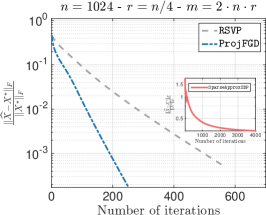
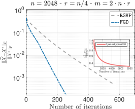
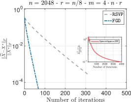
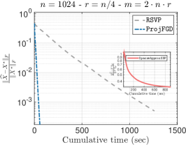
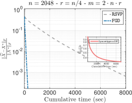
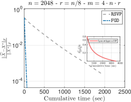
Appendix I Convergence without tail bound assumptions
In this section, we show how assumptions (A3) and (A4) can be dropped by using a different step size , where spectral norm calculation of two matrices is required per iteration. Here, we succinctly describe the main theorems and how they differ from the case where as in (8) is used. We also focus only on the case of restricted strongly convex functions. Similar extension is possible without restricted strong convexity.
Our discussion is organized as follows: we first re-define key lemmas (e.g., descent lemmas, etc.) for a different step size; then, we state the main theorems and a sketch of their proof. In the analysis below we use as step size:
I.1 Key lemmas
Next, we present the main descent lemma that is used for both sublinear and linear convergence rate guarantees of Fgd.
Lemma I.1 (Descent lemma).
For being a -smooth and -strongly convex function and under assumptions and , the following inequality holds true:
Proof of Lemma I.1.
By (13), we have:
| (50) |
Step I: Bounding . For this term, we have a variant of Lemma 6.2, as follows:
Lemma I.2.
Let be a -smooth and -restricted strongly convex function with optimum point . Assume . Let . Then,
where .
The proof of this lemma is provided in Section J.1.
Step II: Bounding . For the second term, we have the following variant of Lemma 6.3.
Lemma I.3.
Let be -smooth and -restricted strongly convex. Then, under assumptions and , the following bound holds true:
Proof of this lemma can be found in Section J.2.
Step III: Combining the bounds in equation (50). The rest of the proof is similar to that of Lemma 6.1.
∎
I.2 Proof of linear convergence
For the case of (restricted) strongly convex functions , we have the following revised theorem:
Theorem I.4 (Convergence rate for restricted strongly convex ).
Let current iterate be and . Assume and let the step size be . Then under assumptions and , the new estimate satisfies
| (51) |
where . Furthermore, satisfies
Appendix J Main lemmas for convergence proof without tail bound assumptions
J.1 Proof of Lemma I.2
Let and . By smoothness of , we get:
| (52) |
where follows from hypothesis of the lemma and since is a feasible point for problem (1). Finally, since , by the -restricted strong convexity of , we get,
| (53) |
Combining equations (52) and (53), we obtain:
| (54) |
instead of (25) in the proof where is used. The rest of the proof follows the same motions with that of Lemma 6.2 and we get:
Moreover, for the case where is just -smooth and , the above bound becomes:
This completes the proof.
J.2 Proof of Lemma I.3
Similar to Lemma 6.3, we have:
At this point, we desire to introduce strong convexity parameter and condition number in our bound. In particular, to bound term , we observe that or . This results into bounding as follows:
Combining the above inequalities, we obtain:
| (55) |
where follows from , is due to Lemma A.3 and bounding by the hypothesis of the lemma, is due to by Lemma A.3, and . Finally, follows from substituting and using Lemma A.3.