A general class of spreading processes with non-Markovian dynamics

Abstract

In this paper we propose a general class of models for spreading processes we call the $SI^{*}V^{*}$ model. Unlike many works that consider a fixed number of compartmental states, we allow an arbitrary number of states on arbitrary graphs with heterogeneous parameters for all nodes and edges. As a result, this generalizes an extremely large number of models studied in the literature including the MSEIV, MSEIR, MSEIS, SEIV, SEIR, SEIS, SIV, SIRS, SIR, and SIS models. Furthermore, we show how the $SI^{*}V^{*}$ model allows us to model non-Poisson spreading processes letting us capture much more complicated dynamics than existing works such as information spreading through social networks or the delayed incubation period of a disease like Ebola. This is in contrast to the overwhelming majority of works in the literature that only consider spreading processes that can be captured by a Markov process. After developing the stochastic model, we analyze its deterministic mean-field approximation and provide conditions for when the disease-free equilibrium is stable. Simulations illustrate our results.

I Introduction

The study of spreading processes on complex networks has recently gained a massive surge of interest. With the wide range of applications including the spreading of a computer virus, how a product is adopted by a marketplace, or how an idea or belief is propagated through a social network, it is no surprise that a plethora of different models and studies have been devoted to this. However, an overwhelming majority of the stochastic models proposed and studied assume that transitions from one state to another (e.g., a healthy individual recovering from a disease) is a Poisson process that follows an exponential distribution. Unfortunately, this simplifying assumption restricts the applicability of such models to exclude a number of specific processes like how information is disseminated through Twitter or how the Ebola virus is spreading in West Africa.

In this paper we propose a very general class of epidemic models and show how it can be used to study spreading processes that don’t necessarily evolve according to an exponential distribution. In addition to being able to account for non-Poisson spreading processes, our model generalizes almost every model studied in the literature including the MSEIV, MSEIR, MSEIS, SEIV, SEIR, SEIS, SIV, SIRS, SIR, and SIS models. The development and analysis of such a general model also allows rapid prototyping of future spreading processes that might not even exist today.

Literature review

One of the oldest and most commonly studied spreading models is the Susceptible-Infected-Susceptible (SIS) model [1]. Early works such as the one above often consider simplistic assumptions such as all individuals in a population being equally likely to interact with everyone else in the population [2]. One of the first works to consider a continuous-time SIS model over arbitrary contact graphs using mean field theory is [3], which provides conditions on when the disease-free state of the system is globally asymptotically stable.

In addition to the simple SIS model, a myriad of different models have also been proposed and studied in the literature. In [4, 5], the authors add various states to model how humans might adapt their behavior when given knowledge about the possibility of an emerging epidemic. The work [6] considers the possible effect of human behavior changes for the three state Susceptible-Alert-Infected-Susceptible (SAIS) model. In [7], a four-state generalized Susceptible-Exposed-Infected-Vigilant (G-SEIV) model is proposed and studied. This model is appealing because it was shown to generalize a large number of other models already studied in the literature [8, 9]. These models have been used to study the propagation of computer viruses [10, 11] or products and information [12], and of course the spreading of diseases [13]. However, a large drawback is that all of the works above consider an underlying Markov process that drives the system.

While this may be well suited for a number of spreading processes, they have also been applied in areas for which this is not a very good approximation. A notable example is the spreading of the Ebola virus. The work [14] looks at the spreading of Ebola in Congo and Uganda in 2004 and estimates the spreading properties of the virus fitted to a four-state SEIR model. Similarly, the work [15] looks at the more recent outbreak of Ebola in West Africa and again estimates the parameters of the virus fitted to a six-state model. The larger number of states allows the model to better capture things like human behavioral changes and also the incubation period of the Ebola virus. However, just like all the works mentioned above, all transitions are assumed to evolve according to an exponential distribution. More specifically, once an individual is exposed to the virus at some time $t_{0}$, the probability that the individual has started showing symptoms by time $t$ is given by $P(t)=1-e^{-\varepsilon(t-t_{0})}$ for some $\varepsilon>0$. However, this is far from a good approximation when looking at the empirical data collected over the years. The work [16] studies a certain strain (Zaire) of the Ebola virus and concludes that the incubation period of the disease is much better modelled as a log-normal distribution with a mean of 12.7 days and standard deviation of 4.31 days, which cannot be well captured by the exponential distribution above. Another prominent example today is the spreading of information through social networks on the internet, such as Twitter or Digg. It has been observed multiple times that the spreading of information in these networks is again better modelled as a log-normal distribution rather than an exponential one [17, 18, 19].

We are only aware of very few works that have considered spreading processes without exponential distributions. The work [20] studies the drastic effects that non-exponential distributions can have both on the speed of the spreading and on the threshold conditions for when the disease will die out or persist. A simple SI model is studied in [21] without the complexity of an arbitrary graph structure. The SIS model with general infection and recovery times is considered in [22]. In this work we generalize this idea to a much wider class of epidemic models.

Statement of contributions

The contributions of this paper are threefold. First, we propose the $SI^{*}V^{*}$ model that generalizes a very large number of models studied in the literature today. Our model allows an arbitrary number of ‘infected’ and ‘vigilant’ states unlike many models that have a fixed number of states. Multiple infected states allows us to capture various stages of a disease or spreading process which may have very different properties in terms of contagiousness, chance of recovery, etc. Multiple vigilant states allows us to capture different reasons that an individual might not be susceptible to a disease including behavioral changes, vaccinations, or even death. Second, we develop and analyze the deterministic mean-field approximation for the model and provide conditions for which the disease-free states of our model are globally asymptotically stable. Finally, we show how allowing our Markov model to have an arbitrary number of states can be used to approximate non-Poisson spreading processes with arbitrary accuracy. This allows us to much more accurately describe real-life phenomena, such as the propagation of information through social networks or spreading of the Ebola virus, which have recently been shown to evolve according to log-normal distributions rather than exponential ones.

Organization

We begin in Section II by reviewing some preliminary concepts that will be useful in the remainder of the paper. We develop our proposed $SI^{*}V^{*}$ model in Section III and analyze its stability properties in Section IV. In Section V we show how our general class of models can be used to model many stochastic spreading processes with state transition times that do not obey an exponential distribution. We demonstrate the efficacy of our model and validate our stability results through simulations of the spreading of the Ebola virus in Section VI. Finally, we gather our concluding remarks and ideas for future work in Section VII.

II Preliminaries

We denote by and $\mathbb{R}_{\geq 0}$ the sets of real and nonnegative real numbers, respectively. We define the indicator function $\mathbf{1}_{Z}$ to be $1$ if $Z$ is true, and $0$ otherwise.

Graph theory

Given a directed graph ${\mathcal{G}}$ with $N$ nodes, we denote by $A\in^{N\times N}$ the associated adjacency matrix. The components of $A$ are given by $a_{ji}=1$ if and only if there exists a directed edge from $i$ to $j$ on the graph ${\mathcal{G}}$. We denote the in-neighbors and out-neighbors of node $i$ as ${\mathcal{N}}^{\text{in}}_{i}=\{j\in\{1,\dots,N\}\,|\,a_{ij}=1\}$ and ${\mathcal{N}}^{\text{out}}_{i}=\{j\in\{1,\dots,N\}\,|\,a_{ji}=1\}$, respectively.

Given a vector $q\in^{n}$, we let $\operatorname{diag}\left(q_{1},\dots,q_{n}\right)$ denote the $n\times n$ diagonal matrix with $q_{1},\dots,q_{n}$ on the diagonal. Given an arbitrary matrix $Q\in^{m\times n}$, we define $\deg(Q)=\operatorname{diag}\left(\sum_{j=1}^{n}q_{1j},\dots,\sum_{j=1}^{n}q_{mj}\right)$ the diagonal $m\times m$ matrix with row sums of $Q$ on the diagonal. For a square matrix $Q$, we define the Laplacian ${\mathcal{L}}(Q)=\deg(Q)-Q$. A square matrix $Q$ is Metzler if its components $q_{ij}\geq 0$ for all $i\neq j$. The following result will be useful in our analysis later.

Lemma II.1 (Properties of Metzler matrices [23, 24])

Given a Metzler matrix $Q$, the following statements are equivalent:

1. $Q$ is Hurwitz

2. There exists a positive vector $v$ such that $Qv<0$

3. There exists a positive vector $w$ such that $w^{T}Q<0$

4. $Q$ is nonsingular and $Q^{-1}\leq 0$

III Model description

We begin by formulating the $SI^{*}V^{*}$ that we study in the remainder of the paper. We follow the idea of the N-intertwined SIS model developed in [25] and its extensions to the SAIS and generalized SEIV models developed in [6, 7]. Although the latter models have been shown to generalize many different models studied in the literature, they assume a fixed number of compartments for a given disease. Instead, we build on a compartmental model studied in [26] in which the number of states relating to the disease are arbitrary. Unlike the population model (i.e., no graph structure) studied in [26], we are interested in proposing and analyzing this model applied to arbitrary networks. In Section V we show how this model can be used to approximate a wide class of spreading processes on networks for any type of state transitions with arbitrary accuracy, rather than only Poisson processes (exponential distributions).

We consider a virus spreading model with three classes of states called the $SI^{*}V^{*}$ model. The first class has only one state which is the susceptible state $S$. The susceptible state $S$ corresponds to a healthy individual who is capable of being exposed to the disease. The second class has $m>0$ states known as infectious states $I$. In the infectious class, an individual can be in any of the $m$ states given by $I^{k}$ for $k\in\{1,\dots,m\}$. This allows the possibility to model a number of variations to the infectious state including human behavior, severity of the disease, etc. The last class has $n>0$ states known as vigilant states $V$. In the vigilant class, an individual can be in any of the $n$ states given by $V^{\ell}$ for $\ell\in\{1,\dots,n\}$. The vigilant class captures individuals who are not infected, but also not immediately susceptible to contract the disease. The various states in the class can be used to model different reasons that the individual is not susceptible such as being vaccinated, having just recovered, or even deceased.

Consider a network with with $N$ nodes. For each node $i\in\{1,\dots,N\}$ we define the random variable $X_{i}(t)\in\{S,I^{1},\dots,I^{m},V^{1},\dots,V^{n}\}$ as the state of node $i$ at a given time $t$. We consider a general directed contact graph ${\mathcal{G}}$ over which the disease can spread. A susceptible node is only able to become exposed if it has at least one neighbor that is in any of the infectious states. A node $i$ can only be infected by nodes in ${\mathcal{N}}^{\text{in}}_{i}$ and can only infect nodes in ${\mathcal{N}}^{\text{out}}_{i}$.

$\delta^{k\ell}_{i}$	Recovery rate from $I^{k}$ to $V^{\ell}$
$\varepsilon^{kk^{\prime}}_{i}$	Infection internal transition rate from $I^{k}$ to $I^{k^{\prime}}$
$\mu_{i}^{\ell\ell^{\prime}}$	Vigilant internal transition rate from $V^{\ell}$ to $V^{\ell^{\prime}}$
$\gamma^{\ell}_{i}$	Rate of becoming susceptible from $V^{\ell}$ to $S$
$\theta^{\ell}_{i}$	Rate of becoming vigilant from $S$ to $V^{\ell}$
$\beta_{ij}^{k}$	Infection rate due to infected $(I^{k})$ neighbor $j$ from $S$ to $I^{1}$

TABLE I: Parameter definitions

The compartmental Markov process is defined by the following parameters. Let $\delta^{k\ell}_{i}$ be the recovery rate of node $i$ going from infectious state $I^{k}$ to vigilant state $V^{\ell}$. This allows the possibility to model different recovery rates depending on which state of an infection the individual is in and which vigilant state the individual will end up in. We let $D_{i}=[\delta^{k\ell}_{i}]_{k\ell}\in^{m\times n}$ be the matrix that describes these transitions. Let $\varepsilon_{i}^{kk^{\prime}}$ be the rate at which an individual in infectious state $I^{k}$ moves to infectious state $I^{k^{\prime}}$. This can model the various different stages or severity of a disease and how individuals move from one stage to another. We let $E_{i}=[\varepsilon_{i}^{kk^{\prime}}]_{kk^{\prime}}\in^{m\times m}$ be the matrix that describes these transitions. We denote by $\mu_{i}^{\ell\ell^{\prime}}$ the internal transition rate from vigilant state $V^{\ell}$ to $V^{\ell^{\prime}}$. This can model different levels and types of vigilance in individuals, such as behavioral changes, changing medications/vaccines, etc. We let $M_{i}=[\mu^{\ell\ell^{\prime}}_{i}]_{\ell\ell^{\prime}}\in^{n\times n}$ be the matrix that describes these transitions. We denote by $\gamma_{i}^{\ell}$ and $\theta_{i}^{\ell}$ the rates of moving from $V^{\ell}$ to $S$ and $S$ to $V^{\ell}$, respectively. Finally, let $\beta_{ij}^{k}$ be the effect that a neighbor $j\in{\mathcal{N}}^{\text{in}}_{i}$ of node $i$ in state $I^{k}$ has on $i$. The rate that an individual $i$ moves from $S$ to $I^{1}$ is then given by

$$\sum_{k^{\prime}=1}^{m}\sum_{j\in{\mathcal{N}}^{\text{in}}_{i}}\beta_{ij}^{k^{\prime}}Y_{j}^{k^{\prime}},$$

where

$$Y_{j}^{k}(t) =\mathbf{1}_{X_{j}(t)=I^{k}}.$$ (1)

Note that when a susceptible individual $i$ becomes infected, it always moves into the first infectious state $I^{1}$. It is then free to move to the other infectious stages according to $E_{i}$. All the disease parameters are nonnegative. Table I presents the definitions of these parameters for convenience.

The dynamics of the epidemic spread is then modeled using the definition of the infinitesimal generator from [27]. For brevity, we only write out a small subset of the possible transitions,

$$P(X_{i}(t^{\prime})=I^{1}|X_{i}(t)=S,X(t)) =\sum_{k^{\prime}=1}^{m}\sum_{j\in{\mathcal{N}}^{\text{in}}_{i}}\beta_{ij}^{k^{\prime}}Y_{j}^{k^{\prime}}+o,$$

$$P(X_{i}(t^{\prime})=I^{2}|X_{i}(t)=I^{1},X(t)) =\varepsilon_{i}^{12}+o,$$

$$P(X_{i}(t^{\prime})=I^{1}|X_{i}(t)=I^{2},X(t)) =\varepsilon_{i}^{21}+o,$$

$$P(X_{i}(t^{\prime})=V^{\ell}|X_{i}(t)=I^{1},X(t)) =\delta^{1\ell}_{i}+o,$$

where $t^{\prime}=t+\Delta t$ and $o=o(\Delta t)$.

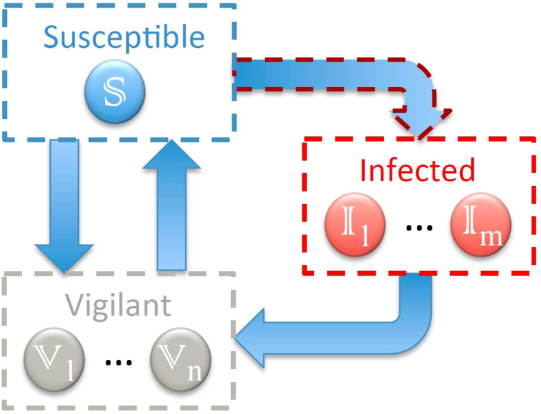
Figure 1 shows the $(1+m+n)$-state $SI^{*}V^{*}$ compartmental Markov model for a single node $i$. Note that the only graph-based transition is from the susceptible state $S$ to the first infected state $I^{1}$. The state of the entire network $X(t)$ then lives in a $(1+m+n)^{N}$ dimensional space making it very hard to analyze directly. Instead, we utilize a mean-field approximation to reduce the complexity of the entire system. We do this by replacing $Y_{j}^{k}$ in (1) by its expected value $E[Y_{j}]^{k}$.

Figure 1: $(1+m+n)$-state $SI^{*}V^{*}$ compartmental model for node $i$. Internal transition rates among the infected and vigilant classes are not shown.

We denote by $\left[S_{i}(t),I_{i}^{1}(t),\dots,I_{i}^{m}(t),V_{i}^{1}(t),\dots,V_{i}^{n}(t)\right]^{T}$ the probability vector associated with node $i$ being in each of these states, i.e.,

$$S_{i}(t)+\sum_{k^{\prime}=1}^{m}I_{i}^{k^{\prime}}(t)+\sum_{\ell^{\prime}=1}^{n}V_{i}^{\ell^{\prime}}(t)=1,$$ (2)

$$S_{i}(t),I_{i}^{k}(t),V_{i}^{\ell}(t)\geq 0,$$

for all $i\in\{1,\dots,N\}$, $k\in\{1,\dots,m\}$, and $\ell\in\{1,\dots,n\}$.

The $SI^{*}V^{*}$ model we consider in this paper is then given by

$$\dot{S}_{i}(t) =\sum_{\ell^{\prime}=1}^{n}\gamma_{i}^{\ell^{\prime}}V_{i}^{\ell^{\prime}}-\theta_{i}^{\ell^{\prime}}S_{i}-S_{i}\sum_{k^{\prime}=1}^{m}\sum_{j\in{\mathcal{N}}^{\text{in}}_{i}}\beta_{ij}^{k^{\prime}}I_{j}^{k^{\prime}},$$

$$\dot{I}_{i}^{1}(t) =S_{i}\sum_{k^{\prime}=1}^{m}\sum_{j\in{\mathcal{N}}^{\text{in}}_{i}}\beta_{ij}^{k^{\prime}}I_{j}^{k^{\prime}}-I_{i}^{1}\sum_{\ell^{\prime}=1}^{n}\delta^{1\ell^{\prime}}_{i}$$

$$\hskip 60.27759pt+\sum_{k^{\prime}=1}^{m}I_{i}^{k^{\prime}}\varepsilon^{k^{\prime}1}_{i}-I_{i}^{1}\varepsilon_{i}^{1k^{\prime}},$$ (3)

$$\dot{I}_{i}^{k}(t) =-I_{i}^{k}\sum_{\ell^{\prime}=1}^{n}\delta^{k\ell^{\prime}}_{i}+\sum_{k^{\prime}=1}^{m}I_{i}^{k^{\prime}}\varepsilon^{k^{\prime}k}_{i}-I_{i}^{k}\varepsilon_{i}^{kk^{\prime}},$$

$$\dot{V}_{i}^{\ell}(t) =\sum_{k^{\prime}=1}^{m}\delta^{k^{\prime}\ell}I_{i}^{k^{\prime}}+\theta^{\ell}_{i}S_{i}-\gamma^{\ell}_{i}V_{i}^{\ell}+\sum_{\ell^{\prime}=1}^{n}V_{i}^{\ell^{\prime}}\mu_{i}^{\ell^{\prime}\ell}-V_{i}^{\ell}\mu_{i}^{\ell\ell^{\prime}},$$

for $k\in\{2,\dots,m\}$ and $\ell\in\{1,\dots,n\}$.

Due to constraints (2), one of the equations (III) is redundant. By setting $S_{i}(t)=1-\sum_{k^{\prime}=1}^{m}I_{i}^{k^{\prime}}(t)-\sum_{\ell^{\prime}=1}^{n}V_{i}^{\ell^{\prime}}(t)$, we can describe the system by

$$\dot{I}_{i}^{1}(t) =(1-\sum_{k^{\prime}=1}^{m}I_{i}^{k^{\prime}}-\sum_{\ell^{\prime}=1}^{n}V_{i}^{\ell^{\prime}})\sum_{k^{\prime}=1}^{m}\sum_{j\in{\mathcal{N}}^{\text{in}}_{i}}\beta_{ij}^{k^{\prime}}I_{j}^{k^{\prime}}$$

$$\hskip 12.91663pt-I_{i}^{1}\sum_{\ell^{\prime}=1}^{n}\delta^{1\ell^{\prime}}_{i}+\sum_{k^{\prime}=1}^{m}I_{i}^{k^{\prime}}\varepsilon^{k^{\prime}1}_{i}-I_{i}^{1}\varepsilon_{i}^{1k^{\prime}},$$

$$\dot{I}_{i}^{k}(t) =-I_{i}^{k}\sum_{\ell=1}^{n}\delta^{k\ell}_{i}+\sum_{k^{\prime}=1}^{m}I_{i}^{k^{\prime}}\varepsilon^{k^{\prime}k}_{i}-I_{i}^{k}\varepsilon_{i}^{kk^{\prime}},$$ (4)

$$\dot{V}_{i}^{\ell}(t) =\sum_{k^{\prime}=1}^{m}\delta^{k^{\prime}\ell}_{i}I_{i}^{k^{\prime}}+\theta^{\ell}_{i}(1-\sum_{k^{\prime}=1}^{m}I_{i}^{k^{\prime}}-\sum_{\ell^{\prime}=1}^{n}V_{i}^{\ell^{\prime}})$$

$$\hskip 12.91663pt-\gamma^{\ell}_{i}V_{i}^{\ell}+\sum_{\ell^{\prime}=1}^{n}V_{i}^{\ell^{\prime}}\mu_{i}^{\ell^{\prime}\ell}-V_{i}^{\ell}\mu_{i}^{\ell\ell^{\prime}}.$$

Next, we are interested in studying the stability properties for this set of $N(m+n)$ ODEs.

IV Stability analysis of $SI^{*}V^{*}$

Let $\mathbf{x}_{i}=\left[I_{i}^{1},\dots,I_{i}^{m}\right]^{T}$, $\mathbf{y}_{i}=\left[V_{i}^{1},\dots,V_{i}^{n}\right]^{T}$, $\mathbf{x}=\left[\mathbf{x}_{1}^{T},\dots,\mathbf{x}_{m}^{T}\right]^{T}$, and $\mathbf{y}=\left[\mathbf{y}_{1}^{T},\dots,\mathbf{y}_{n}^{T}\right]^{T}$. Naturally, we are interested in conditions that will drive the system to a disease-free state, i.e., $\mathbf{x}\rightarrow 0$. We begin by writing the dynamics of the system as

$$\left[\begin{array}[]{c}\mathbf{\dot{x}}\\ \mathbf{\dot{y}}\end{array}\right]={\mathcal{W}}\left[\begin{array}[]{c}\mathbf{x}\\ \mathbf{y}\end{array}\right]+H,$$ (9)

where ${\mathcal{W}}\in^{N(n+m)\times N(n+m)}$ captures the linear part of the dynamics and $H=[H_{x}^{T},H_{y}^{T}]^{T}$, with $H_{x}\in^{Nm}$ and $H_{y}\in^{Nn}$, captures the nonlinear part. For convenience, we split ${\mathcal{W}}$ into smaller matrices such that

$${\mathcal{W}}=\left[\begin{array}[]{cc}{\mathcal{W}}_{xx}&{\mathcal{W}}_{xy}\\ {\mathcal{W}}_{yx}&{\mathcal{W}}_{yy}\end{array}\right].$$

First, we define the matrix ${\mathcal{W}}_{xx}\in^{Nm\times Nm}$ that describes how infected states affect other infected states. Let ${\mathcal{W}}_{xx}=[{\mathcal{W}}_{xx}^{ij}]$ be the block matrix where

$${\mathcal{W}}_{xx}^{ii}=-{\mathcal{L}}(E_{i})-\operatorname{deg}(D_{i})$$

describes the internal transitions between the infected states and the transitions from all infected states to all vigilant states, and

$${\mathcal{W}}^{ij}_{xx}=\left[\begin{array}[]{c}\beta_{ij}^{1},\dots,\beta_{ij}^{m}\\ \mathbf{0}_{(m-1)\times m}\end{array}\right]$$

describes the (linear) transitions of node $i$ from the susceptible state to the first infected state $I^{1}$ due to other nodes. Second, it is easy to see from (III) that ${\mathcal{W}}_{xy}=\mathbf{0}_{Nm\times Nn}$ because the infected states are not (linearly) affected by the vigilant states.

Third, we define the matrix ${\mathcal{W}}_{yx}$ that describes how infected states affect the vigilant states. Since all these transitions happen internally (i.e., do no depend on the network structure), ${\mathcal{W}}_{yx}=[{\mathcal{W}}_{yx}^{ii}]\in^{Nn\times Nm}$ is a block diagonal matrix where

$${\mathcal{W}}_{yx}^{ii}=D_{i}^{T}-\left[\begin{array}[]{ccc}\theta_{i}^{1}&\dots&\theta_{i}^{1}\\ \theta_{i}^{2}&\dots&\theta_{i}^{2}\\ \vdots&&\vdots\\ \theta_{i}^{n}&\dots&\theta_{i}^{n}\end{array}\right]$$

describes the transitions from all infected states to all vigilant states and the transitions from the susceptible state to all vigilant states.

Finally, we define the matrix ${\mathcal{W}}_{yy}\in^{Nn\times Nn}$ that describes how vigilant states affect other vigilant states. As before, since all these transitions happen internally, ${\mathcal{W}}_{yy}=[{\mathcal{W}}_{yy}^{ii}]$ is a block diagonal matrix where

$${\mathcal{W}}_{yy}^{ii}=-{\mathcal{L}}(M_{i})-\left[\begin{array}[]{ccc}\theta_{i}^{1}&\dots&\theta_{i}^{1}\\ \theta_{i}^{2}&\dots&\theta_{i}^{2}\\ \vdots&&\vdots\\ \theta_{i}^{n}&\dots&\theta_{i}^{n}\end{array}\right]-\operatorname{diag}\left(\gamma_{i}^{1},\dots,\gamma_{i}^{m}\right)$$

describes the internal transitions between the vigilant states, transitions from the susceptible state to all vigilant states, and transitions from all vigilant states to the susceptible state.

We now define the column vector $H$. As can be seen in equation (III), the nonlinearities only enter into the dynamics of the first infectious state $I^{1}$. Thus, we can describe $H_{x}^{i}\in^{m}$ as

$$\left[\begin{array}[]{c}\left(-\sum_{k^{\prime}=1}^{m}I_{i}^{k^{\prime}}-\sum_{\ell^{\prime}=1}^{n}V_{i}^{\ell^{\prime}}\right)\sum_{k^{\prime}=1}^{m}\sum_{j\in{\mathcal{N}}^{\text{in}}_{i}}\beta_{ij}^{k^{\prime}}I_{j}^{k^{\prime}}\\ \mathbf{0}_{(m-1)\times 1}\end{array}\right].$$

Due to removing the susceptible state, we also have a constant forcing given by $H_{y}^{i}=\left[\theta^{1}_{i},\dots,\theta^{n}_{i}\right]^{T}\in^{n}$.

Theorem IV.1

(Sufficient condition for global stability of disease-free equilibrium) The disease-free states of (III) are globally asymptotically stable if ${\mathcal{W}}_{xx}$ is Hurwitz.

Proof.

We begin by noticing that ${\mathcal{W}}_{xx}$ is a Metzler matrix. Using Lemma II.1 and the condition that ${\mathcal{W}}_{xx}$ is Hurwitz, we know there exists a positive vector $v\in\mathbb{R}_{>0}^{Nm}$ such that $v^{T}{\mathcal{W}}_{xx}<0$. Consider the Lyapunov function

$$J=v^{T}\mathbf{x},$$

then

$$\dot{J} =v^{T}\mathbf{\dot{x}}$$

$$=v^{T}{\mathcal{W}}_{xx}\mathbf{x}+v^{T}H_{x}$$

$$\leq v^{T}{\mathcal{W}}_{xx}\mathbf{x}$$

is strictly negative for all $\mathbf{x}\neq 0$. It can then easily be shown using LaSalle’s Invariance Principle that $\mathbf{x}\rightarrow 0$ [28]. ∎

Note that this conservative result essentially ignores the vigilant class and how it can help a disease die out. In other words, this result states that if the vigilant class is removed and the disease-free state is still globally asymptotically stable, adding the vigilant class cannot hurt. For this reason, we do not see any forms of the parameters $\mu_{i}^{\ell\ell^{\prime}}$, $\gamma_{i}^{\ell}$, or $\theta_{i}^{\ell}$ appear in the condition.

In order to find the necessary and sufficient condition, we linearize the entire system around the disease-free equilibrium. For simplicity, we assume here that there exists no absorbing state inside the vigilant class. Note that if there exist any absorbing states in the vigilant class, it does not make sense to discuss asymptotic properties anyway, as all individuals will eventually end up there, resulting in a disease-free equilibrium.

We begin by computing the unique equilibrium for the vigilance class states. Letting $\mathbf{\dot{y}}=0$ and $\mathbf{x}=0$, we get

$$\mathbf{y}^{*}=-{\mathcal{W}}_{yy}^{-1}H_{y}.$$

The inverse of ${\mathcal{W}}_{yy}$ is guaranteed to exist because it is a block diagonal matrix made up of negative definite matrices. Let $\left[\bar{V}_{i}^{1},\dots,\bar{V}_{i}^{n}\right]^{T}=\mathbf{y}_{i}^{*}$ for all $i\in\{1,\dots,N\}$. The linearization of (9) around the point $\mathbf{x}=0,\mathbf{y}=\mathbf{y}^{*}$ is then given by

$$\left[\begin{array}[]{c}\mathbf{\dot{x}}\\ \mathbf{\dot{y}}\end{array}\right]={\mathcal{Q}}\left[\begin{array}[]{c}\mathbf{x}\\ \mathbf{y}\end{array}\right],$$

where

$${\mathcal{Q}}_{xx}^{ii}=-{\mathcal{L}}(E_{i})-\deg(D_{i}),$$

$${\mathcal{Q}}^{ij}_{xx}=\left(1-\sum_{\ell^{\prime}=1}^{n}\bar{V}_{i}^{\ell^{\prime}}\right)\left[\begin{array}[]{c}\beta_{ij}^{1},\dots,\beta_{ij}^{m}\\ \mathbf{0}_{(m-1)\times m}\end{array}\right],$$

${\mathcal{Q}}_{xy}={\mathcal{W}}_{xy}=\mathbf{0}_{Nm\times Nn}$, ${\mathcal{Q}}_{yx}={\mathcal{W}}_{yx},$ and ${\mathcal{Q}}_{yy}={\mathcal{W}}_{yy}$.

Theorem IV.2

(Local stability of disease-free equilibrium) The disease-free states of (III) are locally asymptotically stable if and only if ${\mathcal{Q}}_{xx}$ is Hurwitz.

Proof.

Since the linear dynamics of the infectious states $\mathbf{x}$ do not depend on the vigilant states $\mathbf{y}$, we can write

$$\mathbf{\dot{x}}={\mathcal{Q}}_{xx}\mathbf{x}.$$

It is then clear that $\mathbf{x}\rightarrow 0$ in this linearization of the original system if and only if ${\mathcal{Q}}_{xx}$ is Hurwitz. ∎

Remark IV.3

(Global stability of disease-free equilibrium) We conjecture, and verify through simulation, that the necessary and sufficient local stability result of Theorem IV.2 is indeed a global result but it has yet to be shown. We expect to have its proof completed in the near future. $\bullet$

We note here that based on these results, determining the stability properties of the disease-free equilibrium amounts to checking if an $Nm\times Nm$ matrix is Hurwitz, even though the original system is $N(m+n)$-dimensional.

V Non-exponential distributions

In this section we show how existing epidemic models can be studied with non-Markovian state transitions by appropriately constructing an instance of our $SI^{*}V^{*}$ model. To simplify the exposition, we demonstrate this idea for a single example, the spreading of the Ebola virus, but note that the same idea can be used to expand a very large number of different models.

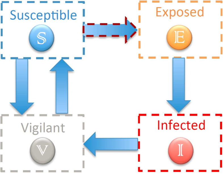
The underlying model we consider is the four-state G-SEIV model proposed in [7] and shown in Figure 2. The ‘Susceptible’ state $S$ captures individuals who are able to be exposed to the disease, the ‘Exposed’ state $E$ captures individuals who have been exposed to the disease but have not yet developed symptoms, the ‘Infected’ state $I$ captures individuals who are displaying symptoms and contagious, and the ‘Vigilant’ state $V$ captures individuals who are not immediately susceptible to the disease (e.g., just recovered, quarantining themselves, deceased).

Figure 2: Four-state G-SEIV compartmental model for node $i$.

We assume that all transitions are Poisson processes except the transition from exposed to infected. For this transition we use a log-normal distribution with mean 12.7 days and standard deviation 4.31 days as proposed in [16] based on empirical data. In the construction of the approximation, an important role is played by the class of probability distributions called phase-type distributions [29].

Consider a time-homogeneous Markov process in continuous-time with $p+1$ ($p\geq 1$) states such that the states $1$, $\dotsc$, $p$ are transient and the state $p+1$ is absorbing. The infinitesimal generator of the process is then necessarily of the form

$$\begin{bmatrix}\SS&-\SS\mathbf{1}_{p\times 1}\\ \mathbf{0}_{1\times p}&0\end{bmatrix},$$ (10)

where $\SS\in\mathbb{R}^{p\times p}$ is an invertible Metzler matrix with non-positive row-sums. Also let

$$\begin{bmatrix}\phi\\ 0\end{bmatrix}\in\mathbb{R}^{p+1},\ \phi\in\mathbb{R}_{\geq 0}^{p}$$ (11)

be the initial distribution of the Markov process. Then, the time to absorption into the state $p+1$ of the Markov process, denoted by $(\phi,\SS)$, is called a phase-type distribution. It is known that the set of phase-type distributions is dense in the set of positive valued distributions [30]. Moreover, there are efficient fitting algorithms to approximate a given arbitrary distribution by a phase-type distribution [29].

We now show how this can be used to expand the G-SEIV model to an instance of our $SI^{*}V^{*}$ model such that the time it takes from to reach the infected state from the exposed state follows a phase-type distribution.

Proposition V.1

Consider the $SI^{*}V^{*}$ model with $m=p+1$ infectious states, where $I^{m}$ corresponds to the infected state and $I^{k}$ for $k\in\{1,\dots,p\}$ correspond to the exposed state. Let $\SS_{I}\in^{m\times m}$ be given by

$$[\SS_{I}]_{kk^{\prime}}=\begin{cases}\varepsilon^{kk^{\prime}}&\text{$k\neq k^{\prime}$},\\ -\sum_{k^{\prime}=1}^{m}\varepsilon^{kk^{\prime}}&\text{otherwise}.\end{cases}$$ (12)

Then the length of time that it takes a node $i$ to go from state $I^{1}$ to $I^{m}$ follows the distribution $(e_{1},S_{I})$, where $e_{1}=\left[1,\mathbf{0}_{1\times p}\right]^{T}$.

Proof.

Without loss of generality, assume that a node $i$ becomes exposed at time $t=0$, i.e., $X_{i}(0)=I^{1}$. Letting $T$ be the time that node $i$ first reaches the infected state, i.e., $X_{i}(T)=I^{m}$, we need to show that $T$ follows $(e_{1},\SS_{I})$.

We begin by noticing that the initial condition $X_{i}(0)=e_{i}$ corresponds to node $i$ having just entered the exposed state. This is because in our $SI^{*}V^{*}$ model, a susceptible node can only enter the infected states through $I^{1}$. Also, from the definition of the model, it is clear that the Markov process $X_{i}$ has the infinitesimal generator (10) on the time interval $[0,T]$. Also $I^{m}$ is clearly the only absorbing state of the process (when confined on $[0,T]$). The above observation shows that $T$ follows the phase-type distribution $(e_{1},\SS_{I})$ because we have satisfied the definitions of the infinitesimal generator (10) and initial distribution (11). ∎

Proposition V.1 shows that it is possible to model the transition from the exposed state to the infected state of the SEIV model as a phase-type distribution. This is done by essentially expanding the exposed state in the original SEIV model from a single state to $p$. As noted earlier, this is only one specific example that can be extended to model many different state transitions as phase-type distributions rather than exponential ones. Next, we show how an arbitrary distribution can be approximated as a phase-type distribution and how to choose the parameters for our $SI^{*}V^{*}$ model to realize the desired distribution.

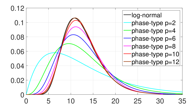
Continuing with our Ebola example, we show how phase-type distributions can well approximate the log-normal distribution of Ebola’s incubation time with mean of $12.7$ days and a standard-deviation of $4.31$ days. To do this, we utilize the expectation-maximization algorithm proposed in [29] Figure 3 shows the results for different amounts of internal states $p$. We can see here that the more internal states $p$ we use, the closer our phase-type distribution becomes to the desired log-normal distribution. An instance of the phase-type distribution for $p=10$ is shown in Figure 4.

Figure 3: Approximation of log-normal distribution (mean 12.7 days and standard deviation 4.31 days) with phase-type distributions for Ebola’s incubation period [16].

Remark V.2

In fact one can show that the set of the phase-type distributions of the form $(e_{1},\SS)$ is dense in the set of all the phase-type distributions as follows. Let $(\phi,\SS)$ be a given phase-type distribution. For a positive real number $r$ define the block-matrix

$$T_{r}=\begin{bmatrix}-r&r\phi^{\top}\\ 0&\SS\end{bmatrix}.$$ (13)

Then we can prove that the sequence of the phase type distributions $\{(e_{1},T_{r})\}_{n=1}^{\infty}$ with $p+2$ states converges to the phase type distribution $(\phi,\SS)$ with $p+1$ states. Here we provide only an outline of the proof. Let $X$ be the time-homogeneous Markov process having the infinitesimal generator (13) and the initial distribution $e_{1}$. Define $t_{1}=\sup\{\tau:X(\tau)=1\}$, i.e., the time at which the Markov process leaves the first state, and let $t_{2}$ be the time the process $X$ is absorbed into the state $p+2$. By the definition of the first row of the generator $T_{r}$, we see that $X(t_{1})$ follows the distribution $\left[0,\phi^{T},0\right]^{T}\in\mathbb{R}_{\geq 0}^{p+2}$.

Therefore $t_{2}-t_{1}$ follows $(\phi,\SS)$. Moreover, as $r$ increases, the probability density function of $t_{1}$ converges to the Dirac delta on the point $0$. Therefore the random variable $t_{2}=t_{1}+(t_{2}-t_{1})$, which follows $(e_{1},T_{r})$ by definition, converges to $(\phi,\SS)$. The details are omitted due to space restrictions. $\bullet$

The implications of Remark V.2 are that although our $SI^{*}V^{*}$ model only allows a susceptible node to enter the infected class through $I^{1}$, we are still able to model any phase-type distribution $(\phi,\SS)$ rather than just $(e_{1},\SS)$.

VI Simulations

Here we demonstrate how the results of Section V can be used to model a spreading process with a non-exponential state transition and validate the stability results of Section IV by simulating the spreading of Ebola. The underlying model we use is a four-state G-SEIV model proposed in [7] and shown in Figure 2. The ‘Susceptible’ state $S$ captures individuals who are able to be exposed to the disease, the ‘Exposed’ state $E$ captures individuals who have been exposed to the disease but have not yet developed symptoms, the ‘Infected’ state $I$ captures individuals who are displaying symptoms and contagious, and the ‘Vigilant’ state $V$ captures individuals who are not immediately susceptible to the disease (e.g., just recovered, quarantining themselves).

We assume that all transitions are Poisson processes except the transition from $E$ to $I$. For this transition we use a log-normal distribution with mean 12.7 days and standard deviation 4.31 days as proposed in [16] based on empirical data. Using the EM algorithm proposed in [29] with $p=10$ phases, we expand the exposed state from a single state to 10 states. This means we can describe our four state non-Poisson SEIV model by a 13-state Poisson $SI^{*}V^{*}$ model with one susceptible state, one vigilant state, and $m=11$ infectious states where $I^{11}$ is the only contagious state. The other infectious states $I^{k}$ for $k\in\{1,\dots,10\}$ correspond to the exposed (but not symptomatic) state of the original SEIV model. The obtained internal compartmental model between the exposed state and infected state is shown in Figure 4.

Figure 4: Approximation of Ebola incubation time distribution with phase-type ($p=10$) distribution.

For our simulations we consider a strongly connected Erdos-Renyi graph $A$ with $N=20$ nodes and connection probability $0.15$. Initially, the vaccination rates $\theta_{i}$ are randomly chosen from a uniform distribution $\theta_{i}\in[0.3,0.8]$ and the rates of becoming susceptible $\gamma_{i}\in[0.2,0.7]$. Since it is known that Ebola can only be transmitted by people who are showing symptoms, we set $\beta_{ij}^{k}=0$ for all $k\in\{1,\dots,10\}$. For links that exist in the graph $A$ we randomly set the infection rate $\beta_{ij}^{11}\in[0.1,0.4]$. Similarly, we assume that only infected individuals can recover, thus we set $\delta_{i}^{k}=0$ for all $k\in\{1,\dots,10\}$ and randomly set the recovery rate $\delta_{i}\in[0.1,0.4]$. Since we only have one vigilant state, there are no internal transition parameters $\mu$.

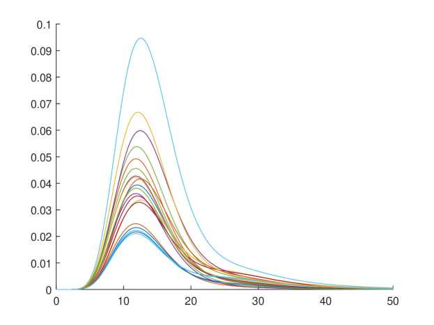
To demonstrate the effectiveness of the expansion of our model to capture the log-normal incubation times of Ebola, we randomly set the initial conditions of being exposed to $I^{1}_{i}(0)\in[0.25,0.75]$ and the susceptible state to $S_{i}(0)=1-I^{1}_{i}(0)$. Thus, we assume that there are initially no nodes in the vigilant $V$ or infected states $I^{k}$ for $k\in\{2,\dots,11\}$. For the parameters used, we obtain $\lambda_{\text{max}}({\mathcal{Q}}_{xx})=-0.1264$ as the largest real part of the eigenvalues of ${\mathcal{Q}}_{xx}$. Figure 5(a) shows the evolution of the maximum, minimum, and average probabilities of being in any of the 11 infected states over time $P_{i}(t)=\sum_{k=1}^{11}I_{i}^{k}(t)$. Figure 5(b) shows the probabilities of being in only the truly infected (and symptomatic) state $I_{i}^{11}(t)$ for all nodes $i$. Here we can see the effectiveness of our expanded model in capturing the log-normal incubation times of Ebola, seeing the peak of infections at 12.7 days. Given enough time, we see that all infections eventually die out as the stability condition of Theorem IV.2 is satisfied.

Figure 5: Plots of (a) the minimum, maximum, and average trajectories of the probability of each node being in any infected state and (b) the trajectories of the probability of each node being in the infectious state $I^{11}$.

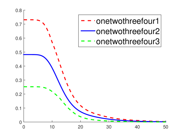
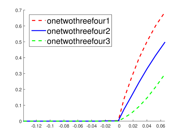
In Figure 6 we vary the recovery rates $\delta_{i}$ and infection rates $\beta_{ij}^{11}$ and look at the steady-state probabilities $P(\infty)$ of each node being in any infectious state where we approximate $P(\infty)\approx P(T)$ for large $T$. We can see here the sharp threshold property that occurs as $\lambda_{\text{max}}({\mathcal{Q}}_{xx})$ moves from negative to positive, validating our stability results of Section IV.

Figure 6: Plot of the minimum, maximum, and average steady-state probabilities of each node being in any infected state.

VII Conclusions

In this work we have proposed a general class of stochastic epidemic models called $SI^{*}V^{*}$ on arbitrary graphs, with heterogeneous node and edge parameters, and an arbitrary number of states. We have then provided conditions for when the disease-free equilibrium of its mean-field approximation is stable. Furthermore, we have shown how this general class of models can be used to handle state transitions that don’t follow an exponential distribution, unlike the overwhelming majority of works in the literature. We demonstrate this modeling capability by simulating the spreading of the Ebola virus, which is known to have a non-exponentially distributed incubation time (i.e., time it takes to show symptoms once an individual is exposed). For future work we are interested in studying how to control this model which can be used in a much wider range of applications than before due to its capabilities in modeling non-Poisson spreading processes.

References

- [1] W. O. Kermack and A. G. McKendrick, “A contribution to the mathematical theory of epidemics,” Proceedings of the Royal Society A, vol. 115, no. 772, pp. 700–721, 1927.
- [2] N. T. Bailey, The Mathematical Theory of Infectious Diseases and its Applications. London: Griffin, 1975.
- [3] A. Lajmanovich and J. A. Yorke, “A deterministic model for gonorrhea in a nonhomogeneous population,” Mathematical Biosciences, vol. 28, no. 3, pp. 221–236, 1976.
- [4] S. Funk, E. Gilad, C. Watkins, and V. A. A. Jansen, “The spread of awareness and its impact on epidemic outbreaks,” Proceedings of the National Academy of Sciences, vol. 16, no. 106, 2009.
- [5] N. Furguson, “Capturing human behaviour,” Nature, vol. 733, no. 446, 2007.
- [6] F. D. Sahneh, F. N. Chowdhury, and C. M. Scoglio, “On the existence of a threshold for preventative behavioral responses to suppress epidemic spreading,” Scientific Reports, vol. 2, no. 632, 2012.
- [7] C. Nowzari, V. M. Preciado, and G. J. Pappas, “Optimal resource allocation in generalized epidemic models,” IEEE Transactions on Control of Network Systems, 2015. Submitted.
- [8] B. A. Prakash, D. Chakrabarti, M. Faloutsos, N. Valler, and C. Faloutsos, “Got the flu (or mumps)? check the eigenvalue!,” arXiv preprint arXiv:1004.0060, 2010.
- [9] H. W. Hethcote, “The mathematics of infectious diseases,” SIAM Review, vol. 42, no. 4, pp. 599–653, 2000.
- [10] M. M. Williamson and J. Leveille, “An epidemiological model of virus spread and cleanup,” in Virus Bulletin, (Toronto, Canada), 2003.
- [11] M. Garetto, W. Gong, and D. Towsley, “Modeling malware spreading dynamics,” in INFOCOM Joint Conference of the IEEE Computer and Communications, pp. 1869–1879, 2003.
- [12] D. Easley and J. Kleinberg, Networks, Crowds, and Markets: Reasoning About a Highly Connected World. Cambridge University Press, 2010.
- [13] M. E. J. Newman, “Spread of epidemic disease on networks,” Physical Review E, vol. 66, p. 016128, 2002.
- [14] G. Chowell, N. W. Hengartner, C. Castillo-Chavez, P. W. Fenimore, and J. M. Hyman, “The basic reproductive number of Ebola and the effects of public health measures: the cases of Congo and Uganda,” Journal of Theoretical Biology, vol. 229, no. 1, pp. 119–126, 2004.
- [15] A. Khan, M. Naveed, M. Dur-e-Ahmad, and M. Imran, “Estimating the basic reproductive ratio for the Ebola outbreak in Liberia and Sierra Leone,” Infectious Diseases of Poverty, vol. 4, no. 13, 2015.
- [16] M. Eichner, S. F. Dowell, and N. Firese, “Incubation period of Ebola hemorrhagic virus subtype Zaire,” Osong Public Health and Research Perspectives, vol. 2, no. 1, 2011.
- [17] K. Lerman, R. Ghosh, and T. Surachawala, “Social contagion: An empirical study of information spread on Digg and Twitter follower graphs,” in Proceedings of the Fourth International AAAI Conference on Weblogs and Social Media, (Washington, DC), pp. 90–97, 2010.
- [18] P. V. Mieghem, N. Blenn, and C. Doerr, “Lognormal distribution in the Digg online social network,” The European Physical Journal B, vol. 83, no. 2, pp. 251–261, 2011.
- [19] C. Doerr, N. Blenn, and P. V. Mieghem, “Lognormal infection times of online information spread,” PLoS ONE, vol. 8, p. e64349, Nov. 2013.
- [20] P. V. Mieghem and R. van de Bovenkamp, “Non-Markovian infection spread dramatically alters the Susceptible-Infected-Susceptible epidemic threshold in networks,” Physical Review Letters, vol. 110, no. 10, p. 108701, 2013.
- [21] H. Jo, J. I. Perotti, K. Kaski, and J. Kertesz, “Analytically solvable model of spreading dynamics with non-Poissonian processes,” Physical Review X, vol. 4, no. 1, p. 011041, 2014.
- [22] E. Cator, R. van de Bovenkamp, and P. V. Mieghem, “Susecptible-Infected-Susceptible epidemics on networks with general infection and cure times,” Physical Review E, vol. 87, p. 062816, 2013.
- [23] A. Rantzer, “Distributed control of positive systems,” in IEEE Conf. on Decision and Control, (Orlando, FL), pp. 6608–6611, 2011.
- [24] L. Farina and S. Rinaldi, Positive Linear Systems. Wiley-Interscience, 2000.
- [25] P. V. Miegham, J. Omic, and R. Kooij, “Virus spread in networks,” IEEE/ACM Transactions on Networking, vol. 17, no. 1, pp. 1–14, 2009.
- [26] M. J. Keeling and P. Rohani, Modeling Infectious Diseases in Humans and Animals. Princeton University Press, 2007.
- [27] P. V. Mieghem, Performance Analysis of Communications Networks and Systems. Cambridge, UK: Cambridge University Press, 2009.
- [28] H. K. Khalil, Nonlinear Systems. Prentice Hall, 3 ed., 2002.
- [29] S. Asmussen, O. Nerman, and M. Olsson, “Fitting phase-type distributions via the EM algorithm,” Scandinavian Journal of Statistic, vol. 23, no. 4, pp. 419–441, 1996.
- [30] D. R. Cox, “A use of complex probabilities in the theory of stochastic processes,” Mathematical Proceedings of the Cambridge Philosophical Society, vol. 51, no. 2, pp. 313–319, 1955.