Two-Sample Smooth Tests for the Equality of Distributions

Wen-Xin Zhou Department of Operations Research and Financial Engineering, Princeton University, Princeton, NJ 08544, USA. E-mail: wenxinz@princeton.edu Chao Zheng School of Mathematics and Statistics, University of Melbourne, Parkville, VIC 3010, Australia. E-mail: zhengc1@student.unimelb.edu.au and Zhen Zhang Department of Statistics, University of Chicago, Chicago, IL 60637, USA. E-mail: zhangz19@galton.uchicago.edu
Abstract

This paper considers the problem of testing the equality of two unspecified distributions. The classical omnibus tests such as the Kolmogorov-Smirnov and Cramér-von Mises are known to suffer from low power against essentially all but location-scale alternatives. We propose a new two-sample test that modifies the Neyman’s smooth test and extend it to the multivariate case based on the idea of projection pursue. The asymptotic null property of the test and its power against local alternatives are studied. The multiplier bootstrap method is employed to compute the critical value of the multivariate test. We establish validity of the bootstrap approximation in the case where the dimension is allowed to grow with the sample size. Numerical studies show that the new testing procedures perform well even for small sample sizes and are powerful in detecting local features or high-frequency components.

Keywords: Neyman’s smooth test; Goodness-of-fit; Multiplier bootstrap; High-frequency alternations; Two-sample problem

1 Introduction

Let X𝑋X and Y𝑌Y be two psuperscript𝑝\mathbb{R}^{p}-valued random variables with continuous distribution functions F𝐹F and G𝐺G, respectively, where p1𝑝1p\geq 1 is a positive integer. Given data from each of the two unspecified distributions F𝐹F and G𝐺G, we are interested in testing the null hypothesis of the equality of distributions

H0:F=G versus H1:FG.:subscript𝐻0𝐹𝐺 versus subscript𝐻1:𝐹𝐺H_{0}:F=G\ \ \mbox{ versus }\ \ H_{1}:F\neq G. (1.1)

This is the two-sample version of the conventional goodness-of-fit problem, which is one of the most fundamental hypothesis testing problems in statistics (Lehmann and Romano, 2005).

1.1 Univariate case: p=1𝑝1p=1

Suppose we have two independent univariate random samples 𝒳n={X1,,Xn}subscript𝒳𝑛subscript𝑋1subscript𝑋𝑛\mathcal{X}_{n}=\{X_{1},\ldots,X_{n}\} and 𝒴m={Y1,,Ym}subscript𝒴𝑚subscript𝑌1subscript𝑌𝑚\mathcal{Y}_{m}=\{Y_{1},\ldots,Y_{m}\} from F𝐹F and G𝐺G, respectively. The empirical distribution functions (EDF) are given by

Fn(x)=1ni=1nI(Xix) and Gm(y)=1mj=1mI(Yjy).formulae-sequencesubscript𝐹𝑛𝑥1𝑛superscriptsubscript𝑖1𝑛𝐼subscript𝑋𝑖𝑥 and subscript𝐺𝑚𝑦1𝑚superscriptsubscript𝑗1𝑚𝐼subscript𝑌𝑗𝑦F_{n}(x)=\frac{1}{n}\sum_{i=1}^{n}I(X_{i}\leq x)\ \ \mbox{ and }\ \ G_{m}(y)=\frac{1}{m}\sum_{j=1}^{m}I(Y_{j}\leq y). (1.2)

For testing the equality of two univariate distributions, conventional approaches in the literature use a measure of discrepancy between Fnsubscript𝐹𝑛F_{n} and Gmsubscript𝐺𝑚G_{m} as a test statistic. Prototypical examples include the Kolmogorov-Smirnov (KS) test Ψ^KS=nm/(n+m)supt|Fn(t)Gm(t)|subscript^ΨKS𝑛𝑚𝑛𝑚subscriptsupremum𝑡subscript𝐹𝑛𝑡subscript𝐺𝑚𝑡\hat{\Psi}_{{\rm KS}}=\sqrt{nm/(n+m)}\sup_{t\in\mathbb{R}}|F_{n}(t)-G_{m}(t)| and the Cramér-von Mises (CVM) family of statistics

Ψ^CVM=nmn+m{Fn(t)Gm(t)}2w(Hn+m(t))𝑑Hn,m(t),subscript^ΨCVM𝑛𝑚𝑛𝑚superscriptsubscriptsuperscriptsubscript𝐹𝑛𝑡subscript𝐺𝑚𝑡2𝑤subscript𝐻𝑛𝑚𝑡differential-dsubscript𝐻𝑛𝑚𝑡\hat{\Psi}_{{\rm CVM}}=\frac{nm}{n+m}\int_{-\infty}^{\infty}\{F_{n}(t)-G_{m}(t)\}^{2}w(H_{n+m}(t))\,dH_{n,m}(t),

where Hn,m(t):={nFn(t)+mGm(t)}/(n+m)assignsubscript𝐻𝑛𝑚𝑡𝑛subscript𝐹𝑛𝑡𝑚subscript𝐺𝑚𝑡𝑛𝑚H_{n,m}(t):=\{nF_{n}(t)+mG_{m}(t)\}/(n+m) denotes the pooled EDF and w𝑤w is a non-negative weight function. Taking w1𝑤1w\equiv 1 yields the Cramér-von Mises statistic, and w(t)={t(1t)}1𝑤𝑡superscript𝑡1𝑡1w(t)=\{t(1-t)\}^{-1} yields the Anderson-Darling statistic (Darling, 1957).

The traditional omnibus tests, which have been widely used for testing the two-sample goodness-of-fit hypothesis (1.1) due to their simplicity with which they can be performed, suffer from low power in detecting densities containing high-frequency components or local features such as bumps, and thus may have poor finite sample power properties (Fan, 1996). It is known from empirical studies that the CVM test has poor power against essentially all but location-scale alternatives (Eubank and LaRiccia, 1992). The same issue arises in the KS test as well. To enhance power under local alternatives, Neyman’s smooth method (Neyman, 1937) was introduced earlier than the traditional omnibus tests, to test only the first d𝑑d-dimensional sub-problem if there is prior that most of the discrepancies fall within the first d𝑑d orthogonal directions. Essentially, Neyman’s smooth tests represent a compromise between omnibus and directional tests. As evidenced by numerous empirical studies over the years, smooth tests have been shown to be more powerful than traditional omnibus tests over a broad range of realistic alternatives. See, for example, Eubank and LaRiccia (1992), Fan (1996), Janssen (2000), Bera and Ghosh (2002) and Escanciano (2009).

A two-sample analogue of the Neyman’s smooth test was recently proposed by Bera, Ghosh and Xiao (2013) for testing the equality of F𝐹F and G𝐺G based on two independent samples. The test statistic is asymptotically chi-square distributed and as a special case of Rao’s score test, it enjoys certain optimality properties. Specifically, Bera, Ghosh and Xiao (2013) motivated the two-sample Neyman’s smooth test by considering the random variable V=F(Y)𝑉𝐹𝑌V=F(Y) with distribution and density functions given by

H(z):=G(F1(z)) and ρ(z):=g(F1(z))/f(F1(z))formulae-sequenceassign𝐻𝑧𝐺superscript𝐹1𝑧 and assign𝜌𝑧𝑔superscript𝐹1𝑧𝑓superscript𝐹1𝑧H(z):=G(F^{-1}(z))\ \ \mbox{ and }\ \ \rho(z):=g(F^{-1}(z))/f(F^{-1}(z)) (1.3)

for 0<z<10𝑧10<z<1, respectively, where F1superscript𝐹1F^{-1} is the quantile function of X𝑋X, i.e. F1(z)=inf{x:F(x)z}superscript𝐹1𝑧infimumconditional-set𝑥𝐹𝑥𝑧F^{-1}(z)=\inf\{x\in\mathbb{R}:F(x)\geq z\}, and f𝑓f and g𝑔g denote the density functions of X𝑋X and Y𝑌Y. Assume that F𝐹F and G𝐺G are strictly increasing, then H𝐻H is also increasing, ρ(z)0𝜌𝑧0\rho(z)\geq 0 for 0<z<10𝑧10<z<1 and 01ρ(z)𝑑z=1superscriptsubscript01𝜌𝑧differential-d𝑧1\int_{0}^{1}\rho(z)\,dz=1. Under the null hypothesis H0subscript𝐻0H_{0}, ρ1𝜌1\rho\equiv 1 so that V=dU(0,1)subscript𝑑𝑉𝑈01V=_{d}U(0,1). In other words, the null hypothesis H0subscript𝐻0H_{0} in (1.1) is equivalent to

H~0:ρ(z)=1 for all 0<z<1,:subscript~𝐻0formulae-sequence𝜌𝑧1 for all 0𝑧1\tilde{H}_{0}:\rho(z)=1\ \ \mbox{ for all }0<z<1, (1.4)

where ρ𝜌\rho is as in (1.3). Throughout, the function ρ𝜌\rho is referred as the ratio density function. Based on Neyman’s smooth test principle, we restrict attention to the following smooth alternatives to the null of uniformity

ρθ(z)=Cd(θ)exp{k=1dθkψk(z)}forθ:=(θ1,,θd)dand 0<z<1,formulae-sequenceformulae-sequencesubscript𝜌𝜃𝑧subscript𝐶𝑑𝜃superscriptsubscript𝑘1𝑑subscript𝜃𝑘subscript𝜓𝑘𝑧forassign𝜃superscriptsubscript𝜃1subscript𝜃𝑑superscript𝑑and 0𝑧1\rho_{\theta}(z)=C_{d}(\theta)\exp\bigg{\{}\sum_{k=1}^{d}\theta_{k}\psi_{k}(z)\bigg{\}}\ \ {\rm for}\ \ \theta:=(\theta_{1},\ldots,\theta_{d})^{\intercal}\in\mathbb{R}^{d}\ \ {\rm and}\ \ 0<z<1, (1.5)

which include a broad family of parametric alternatives, where d=dim(θ)𝑑dim𝜃d=\mbox{dim}(\theta) is some positive integer and {Cd(θ)}1=01exp{k=1dθkψk(z)}𝑑zsuperscriptsubscript𝐶𝑑𝜃1superscriptsubscript01superscriptsubscript𝑘1𝑑subscript𝜃𝑘subscript𝜓𝑘𝑧differential-d𝑧\{C_{d}(\theta)\}^{-1}=\int_{0}^{1}\exp\big{\{}\sum_{k=1}^{d}\theta_{k}\psi_{k}(z)\big{\}}\,dz. Setting ψ01subscript𝜓01\psi_{0}\equiv 1, the functions ψ1,,ψdsubscript𝜓1subscript𝜓𝑑\psi_{1},\ldots,\psi_{d} are chosen in such a way that {ψ0,ψ1,,ψd}subscript𝜓0subscript𝜓1subscript𝜓𝑑\{\psi_{0},\psi_{1},\ldots,\psi_{d}\} forms a set of orthonormal functions, i.e.

01ψk(z)ψ(z)𝑑z=δk={1, if k=,0, if k.superscriptsubscript01subscript𝜓𝑘𝑧subscript𝜓𝑧differential-d𝑧subscript𝛿𝑘cases1 if 𝑘otherwise0 if 𝑘otherwise\int_{0}^{1}\psi_{k}(z)\psi_{\ell}(z)\,dz=\delta_{k\ell}=\begin{cases}1,\ \ \mbox{ if }k=\ell,\\ 0,\ \ \mbox{ if }k\neq\ell.\end{cases} (1.6)

The null hypothesis asserts H0d:θ=0:subscriptsuperscript𝐻𝑑0𝜃0H^{d}_{0}:\theta=0. Assuming that mn𝑚𝑛m\leq n and the truncation parameter d𝑑d is fixed, the two-sample smooth test proposed by Bera, Ghosh and Xiao (2013) is defined as Ψ^BGX=m𝝍^𝝍^subscript^ΨBGX𝑚superscript^𝝍^𝝍\hat{\Psi}_{{\rm BGX}}=m\hat{\boldsymbol{\psi}}^{\intercal}\hat{\boldsymbol{\psi}}, where 𝝍^=m1j=1m𝝍(V^j)^𝝍superscript𝑚1superscriptsubscript𝑗1𝑚𝝍subscript^𝑉𝑗\hat{\boldsymbol{\psi}}=m^{-1}\sum_{j=1}^{m}\boldsymbol{\psi}(\hat{V}_{j}), 𝝍=(ψ1,,ψd)𝝍superscriptsubscript𝜓1subscript𝜓𝑑\boldsymbol{\psi}=(\psi_{1},\ldots,\psi_{d})^{\intercal} and V^j=Fn(Yj)subscript^𝑉𝑗subscript𝐹𝑛subscript𝑌𝑗\hat{V}_{j}=F_{n}(Y_{j}). Under certain moment conditions and if the sample sizes (n,m)𝑛𝑚(n,m) satisfy mloglogn=o(n)𝑚𝑛𝑜𝑛m\log\log n=o(n) as n,m𝑛𝑚n,m\rightarrow\infty, the test statistic Ψ^BGXsubscript^ΨBGX\hat{\Psi}_{{\rm BGX}} converges in distribution to the χ2superscript𝜒2\chi^{2} distribution with d𝑑d degrees of freedom. Accounting for the error of estimating F𝐹F, Bera, Ghosh and Xiao (2013) further considered a generalized version of the smooth test that is asymptotically χ2(d)superscript𝜒2𝑑\chi^{2}(d) distributed and can be applied when n𝑛n and m𝑚m are of the same magnitude.

However, Bera, Ghosh and Xiao (2013) only focused on the fix d𝑑d scenario (i.e. d=4𝑑4d=4) so that their two-sample smooth test is consistent in power against alternative where V=F(Y)𝑉𝐹𝑌V=F(Y) does not have the same first k𝑘k moments as that of the uniform distribution (Lehmann and Romano, 2005). If there is a priori evidence that most of the energy is concentrated at low frequencies, i.e. large θksubscript𝜃𝑘\theta_{k} are located at small k𝑘k, it is reasonable to use Neyman’s smooth test. Otherwise, Neyman’s test is less powerful when testing contiguous alternatives with local characters (Fan, 1996). As Janssen (2000) pointed out, achieving reasonable power over more than a few orthogonal directions is hopeless. Indeed, the larger the value of d𝑑d, the greater the number of orthogonal directions used to construct the test statistic. Therefore, it is possible to obtain consistency against all distributions if the truncation parameter d𝑑d is allowed to increase with the sample size. Motivated by Chang, Zhou and Zhou (2014), we regard H0d:θ=0:subscriptsuperscript𝐻𝑑0𝜃0H^{d}_{0}:\theta=0 as a global mean testing problem with dimension increasing with the sample size. When d𝑑d is large, Neyman’s smooth test which is based on the 2subscript2\ell_{2}-norm of θ𝜃\theta may also suffer from low powers under sparse alternatives. In part, this is because that the quadratic statistic accumulates high-dimensional estimation errors under H0dsubscriptsuperscript𝐻𝑑0H^{d}_{0}, resulting in large critical values that can dominate the signals under sparse alternatives.

To overcome the foregoing drawbacks, we first note that the traditional omnibus tests aim to capture the differences of two entire distributions as opposed to only assessing a particular aspect of the distributions, by contrast, Neyman’s smooth principle reduces the original nonparametric problem to a d𝑑d-dimensional parametric one. Lying in the middle, we are interested in enhancing the power in detecting two adjacent densities where one has local features or contains high-frequency components, while maintaining the same capability in detecting smooth alternative densities as the traditional tests. We expect to arrive at a compromise between desired significance level and statistical power by allowing the truncation parameter d𝑑d to increase with sample sizes. In Section 2, we introduce a new test statistic by taking maximum over d𝑑d univariate statistics. The limiting null distribution is derived under mild conditions, while d𝑑d is allowed to grow with n𝑛n and m𝑚m. To conduct inference, a novel intermediate approximation to the null distribution is proposed to compute the critical value. In fact, when n𝑛n and m𝑚m are comparable, d𝑑d can be of order n1/4superscript𝑛14n^{1/4} (resp. n1/9superscript𝑛19n^{1/9}) (up to logarithmic in n𝑛n factors) if the trigonometric series (resp. Legendre polynomial series) is used to construct the test statistic.

1.2 Multivariate case: p2𝑝2p\geq 2

As a canonical problem in multivariate analysis, testing the equality of two multivariate distributions based on the two samples has been extensively studied in the literature that can be dated back to Weiss (1960), under the conventional fix p𝑝p setting. Friedman and Rafsky (1979) constructed a two-sample test based on the minimal spanning tree formed from the interpoint distances and their test statistic was shown to be asymptotically distribution free under the null; Schilling (1986) and Henze (1988) proposed nearest neighbor tests which are based on the number of times that the nearest netghbors come from the same group; Rosenbaum (2005) proposed an exact distribution-free test based on a matching of the observations into disjoint pairs to minimize the total distance within pairs. Work in the context of nonparametric tests include that of Hall and Tajvidi (2002), Baringhaus and Franz (2004, 2010) and Biswas and Ghosh (2014), among others.

Most aforementioned existing methods are tailored for the case where the dimension p𝑝p is fixed. Driven by a broad range of contemporary statistical applications, analysis of high-dimensional data is of significant current interest. In the high-dimensional setting, the classical testing procedures may have poor power performance, as evidenced by the numerical investigations in Biswas and Ghosh (2014). Several tests for the equality of two distributions in high dimensions have been proposed. See, for example, Hall and Tajvidi (2002) and Biswas and Ghosh (2014). However, limiting null distributions of the test statistics introduced in Hall and Tajvidi (2002) and Biswas and Ghosh (2014) were derived when the dimension p𝑝p is fixed.

In the present paper, we propose a new test statistic that extends Neyman’s smooth test principle to higher dimensions based on the idea of projection pursue. To conduct inference for the test, we employ the multiplier (wild) bootstrap method which is similar in spirit to that used in Hansen (1996) and Barrett and Donald (2003). We refer to Section 3 for details on methodologies. It can be shown that (Propositions 7.2 and 7.3), under mild conditions, the error in size of our multivariate smooth test decays polynomially in sample sizes (n,m)𝑛𝑚(n,m). It is noteworthy that we allow the dimension p𝑝p to grow as a function of (n,m)𝑛𝑚(n,m), a type of framework the existing methods do not rigorously address. More importantly, we do not limit the dependency structure among the coordinates in X𝑋X and Y𝑌Y and no shape constraints of the distribution curves are known as a priori which inhibits a pure parametric approach to the problem.

1.3 Organization of the paper

The rest of the paper is organized as follows. In Section 2, we describe the two-sample smooth testing procedure in the univariate case. An extension to the multivariate setting based on projection pursue is introduced in Section 3. Section 4 establishes theoretical properties of the proposed smooth tests in both univariate and multivariate settings. Finite sample performance of the proposed tests is investigated in Section 5 through Monte Carlo experiments. The proofs of the main results are given in Section 7 and some additional technical arguments are contained in the Appendix.

Notation. For a positive integer p𝑝p, we write [p]={1,2,,p}delimited-[]𝑝12𝑝[p]=\{1,2,\ldots,p\} and denote by ||2|\cdot|_{2} and |||\cdot|_{\infty} the 2subscript2\ell_{2}- and subscript\ell_{\infty}-norm in psuperscript𝑝\mathbb{R}^{p}, respectively, i.e. |x|2=(x12++xp2)1/2subscript𝑥2superscriptsuperscriptsubscript𝑥12superscriptsubscript𝑥𝑝212|x|_{2}=(x_{1}^{2}+\cdots+x_{p}^{2})^{1/2} and |x|=maxk[p]|xk|subscript𝑥subscript𝑘delimited-[]𝑝subscript𝑥𝑘|x|_{\infty}=\max_{k\in[p]}|x_{k}| for x=(x1,,xp)p𝑥superscriptsubscript𝑥1subscript𝑥𝑝superscript𝑝x=(x_{1},\ldots,x_{p})^{\intercal}\in\mathbb{R}^{p}. The unit sphere in psuperscript𝑝\mathbb{R}^{p} is denoted by 𝒮p1={xp:|x|2=1}superscript𝒮𝑝1conditional-set𝑥superscript𝑝subscript𝑥21\mathcal{S}^{p-1}=\{x\in\mathbb{R}^{p}:|x|_{2}=1\}. For two psuperscript𝑝\mathbb{R}^{p}-valued random variables X𝑋X and Y𝑌Y, we write X=dYsubscript𝑑𝑋𝑌X=_{d}Y if they have the same probability distribution and denote by PXsubscript𝑃𝑋P_{X} the probability measure on psuperscript𝑝\mathbb{R}^{p} induced by X𝑋X. For two real numbers a𝑎a and b𝑏b, we use the notation ab=max(a,b)𝑎𝑏𝑎𝑏a\vee b=\max(a,b) and ab=min(a,b)𝑎𝑏𝑎𝑏a\wedge b=\min(a,b). For two sequences of positive numbers ansubscript𝑎𝑛a_{n} and bnsubscript𝑏𝑛b_{n}, we write anbnasymptotically-equalssubscript𝑎𝑛subscript𝑏𝑛a_{n}\asymp b_{n} if there exist constants c1,c2>0subscript𝑐1subscript𝑐20c_{1},c_{2}>0 such that for all sufficiently large n𝑛n, c1an/bnc2subscript𝑐1subscript𝑎𝑛subscript𝑏𝑛subscript𝑐2c_{1}\leq a_{n}/b_{n}\leq c_{2}, we write an=O(bn)subscript𝑎𝑛𝑂subscript𝑏𝑛a_{n}=O(b_{n}) if there is a constant C>0𝐶0C>0 such that for all n𝑛n large enough, anCbnsubscript𝑎𝑛𝐶subscript𝑏𝑛a_{n}\leq Cb_{n}, and we write anbnsimilar-tosubscript𝑎𝑛subscript𝑏𝑛a_{n}\sim b_{n} or anbnsimilar-to-or-equalssubscript𝑎𝑛subscript𝑏𝑛a_{n}\simeq b_{n} and an=o(bn)subscript𝑎𝑛𝑜subscript𝑏𝑛a_{n}=o(b_{n}), respectively, if limnan/bn=1subscript𝑛subscript𝑎𝑛subscript𝑏𝑛1\lim_{n\rightarrow\infty}a_{n}/b_{n}=1 and limnan/bn=0subscript𝑛subscript𝑎𝑛subscript𝑏𝑛0\lim_{n\rightarrow\ \infty}a_{n}/b_{n}=0. For any two functions f,g::𝑓𝑔maps-tof,g:\mathbb{R}\mapsto\mathbb{R}, we denote with fg𝑓𝑔f\circ g the composite function fg(x)=f{g(x)}𝑓𝑔𝑥𝑓𝑔𝑥f\circ g(x)=f\{g(x)\} for x𝑥x\in\mathbb{R}.

For any probability measure Q𝑄Q on a measurable space (𝕊,𝒮)𝕊𝒮(\mathbb{S},\mathcal{S}), let Q,2\|\cdot\|_{Q,2} be L2(Q)subscript𝐿2𝑄L_{2}(Q)-seminorm defined by fQ,2=(Q|f|2)1/2=(|f|2𝑑Q)1/2subscriptnorm𝑓𝑄2superscript𝑄superscript𝑓212superscriptsuperscript𝑓2differential-d𝑄12\|f\|_{Q,2}=(Q|f|^{2})^{1/2}=(\int|f|^{2}\,dQ)^{1/2} for fL2(Q)𝑓subscript𝐿2𝑄f\in L_{2}(Q). For a class of measurable functions \mathcal{F} equipped with an envelope F(s)=supf|f(s)|𝐹𝑠subscriptsupremum𝑓𝑓𝑠F(s)=\sup_{f\in\mathcal{F}}|f(s)| for s𝕊𝑠𝕊s\in\mathbb{S}, let N(,L2(Q),εFQ,2)𝑁subscript𝐿2𝑄𝜀subscriptnorm𝐹𝑄2N(\mathcal{F},L_{2}(Q),\varepsilon\|F\|_{Q,2}) denote the ε𝜀\varepsilon-covering number of the class of functions \mathcal{F} with respect to the L2(Q)subscript𝐿2𝑄L_{2}(Q)-distance for 0<ε10𝜀10<\varepsilon\leq 1. We say that the class \mathcal{F} is Euclidean or VC-type (Nolan and Pollard, 1987; van der Vaart and Wellner, 1996) if there are constants A,v>0𝐴𝑣0A,v>0 such that supQN(,L2(Q),εFQ,2)(A/ε)vsubscriptsupremum𝑄𝑁subscript𝐿2𝑄𝜀subscriptnorm𝐹𝑄2superscript𝐴𝜀𝑣\sup_{Q}N(\mathcal{F},L_{2}(Q),\varepsilon\|F\|_{Q,2})\leq(A/\varepsilon)^{v} for all 0<ε10𝜀10<\varepsilon\leq 1, where the supremum ranges over over all finitely discrete probability measures on (𝕊,𝒮)𝕊𝒮(\mathbb{S},\mathcal{S}). When 𝕊=p𝕊superscript𝑝\mathbb{S}=\mathbb{R}^{p} for p1𝑝1p\geq 1, we use 𝒮𝒮\mathcal{S} to denote the Borel σ𝜎\sigma-algebra unless otherwise stated.

2 Testing equality of two univariate distributions

2.1 Oracle procedure

Without loss of generality, we assume nm𝑛𝑚n\geq m and recall that the null hypothesis H0:F=G:subscript𝐻0𝐹𝐺H_{0}:F=G is equivalent to H~0:V=dU(0,1):subscript~𝐻0subscript𝑑𝑉𝑈01\tilde{H}_{0}:V=_{d}U(0,1) for V=F(Y)𝑉𝐹𝑌V=F(Y) as in (1.4). Following Bera, Ghosh and Xiao (2013), we consider the smooth alternatives lying in the family of densities (1.5) which is a d𝑑d-parameter exponential family, where d=dn,m𝑑subscript𝑑𝑛𝑚d=d_{n,m} is allowed to increase with n𝑛n and m𝑚m in order to obtain power against a large array of alternatives. In particular, this family is quadratic mean differentiable at θ=0𝜃0\theta=0 and therefore the score vector at θ=0𝜃0\theta=0 is given by m1/2(θ1logLm(θ),,θdlogLm(θ))|θ=0evaluated-atsuperscript𝑚12subscript𝜃1subscript𝐿𝑚𝜃subscript𝜃𝑑subscript𝐿𝑚𝜃𝜃0m^{-1/2}\big{(}\frac{\partial}{\partial\theta_{1}}\log L_{m}(\theta),\ldots,\frac{\partial}{\partial\theta_{d}}\log L_{m}(\theta)\big{)}|_{\theta=0} (Lehmann and Romano, 2005), where Lm(θ)={Cd(θ)}mexp{j=1mk=1dθkψk(Vj)}subscript𝐿𝑚𝜃superscriptsubscript𝐶𝑑𝜃𝑚superscriptsubscript𝑗1𝑚superscriptsubscript𝑘1𝑑subscript𝜃𝑘subscript𝜓𝑘subscript𝑉𝑗L_{m}(\theta)=\{C_{d}(\theta)\}^{m}\exp\big{\{}\sum_{j=1}^{m}\sum_{k=1}^{d}\theta_{k}\psi_{k}(V_{j})\big{\}} is the likelihood function and Vj=F(Yj)subscript𝑉𝑗𝐹subscript𝑌𝑗V_{j}=F(Y_{j}), such that θklogLm(θ)=j=1m[ψk(Vj)Eθ{ψk(Vj)}]subscript𝜃𝑘subscript𝐿𝑚𝜃superscriptsubscript𝑗1𝑚delimited-[]subscript𝜓𝑘subscript𝑉𝑗subscript𝐸𝜃subscript𝜓𝑘subscript𝑉𝑗\frac{\partial}{\partial\theta_{k}}\log L_{m}(\theta)=\sum_{j=1}^{m}[\psi_{k}(V_{j})-E_{\theta}\{\psi_{k}(V_{j})\}]. As {ψ01,ψ1,,ψd}subscript𝜓01subscript𝜓1subscript𝜓𝑑\{\psi_{0}\equiv 1,\psi_{1},\ldots,\psi_{d}\} forms a set of orthonormal functions, it is easy to see that if θ=0𝜃0\theta=0, Eθ{ψk(V)}=0subscript𝐸𝜃subscript𝜓𝑘𝑉0E_{\theta}\{\psi_{k}(V)\}=0 and Eθ{ψk(V)2}=1subscript𝐸𝜃subscript𝜓𝑘superscript𝑉21E_{\theta}\{\psi_{k}(V)^{2}\}=1 for every k[d]𝑘delimited-[]𝑑k\in[d].

To provide a more omnibus test against a broader range of alternatives, we allow a large truncation parameter d𝑑d and for the reduced null hypothesis H0d:θ=0:subscriptsuperscript𝐻𝑑0𝜃0H^{d}_{0}:\theta=0, it is instructive to consider the following oracle statistic

Ψ(d)=max1kd|1mj=1mψk(Vj)|,Ψ𝑑subscript1𝑘𝑑1𝑚superscriptsubscript𝑗1𝑚subscript𝜓𝑘subscript𝑉𝑗\Psi(d)=\max_{1\leq k\leq d}\bigg{|}\frac{1}{\sqrt{m}}\sum_{j=1}^{m}\psi_{k}(V_{j})\bigg{|}, (2.1)

which can be regarded as a smoothed version of the KS statistic. Throughout, the number of orthogonal directions d=dim(θ)𝑑dim𝜃d=\mbox{dim}(\theta) is chosen such that dnm𝑑𝑛𝑚d\leq n\wedge m. Intuitively, this extreme value statistic is appealing when most of the energy (non-zero θksubscript𝜃𝑘\theta_{k}) is concentrated on a few dimensions but with unknown locations, meaning that both low- and high-frequency alternations are possible. Now it is a common belief (Cai, Liu and Xia, 2014) that maximum-type statistics are powerful against sparse alternatives, which in the current context is the case where the two densities only differ in a small number of orthogonal directions (not necessarily in the first few). To see this, consider a contiguous alternative where there exists some superscript\ell^{*} such that θ0subscript𝜃superscript0\theta_{\ell^{*}}\neq 0 with |θ|subscript𝜃superscript|\theta_{\ell^{*}}| sufficiently small and θ=0subscript𝜃0\theta_{\ell}=0 for all other \ell, then informally we have Cd1(θ)=01exp{θψ(z)}𝑑z01{1+θψ(z)}𝑑z=1superscriptsubscript𝐶𝑑1𝜃superscriptsubscript01subscript𝜃superscriptsubscript𝜓superscript𝑧differential-d𝑧similar-to-or-equalssuperscriptsubscript011subscript𝜃superscriptsubscript𝜓superscript𝑧differential-d𝑧1C_{d}^{-1}(\theta)=\int_{0}^{1}\exp\{\theta_{\ell^{*}}\psi_{\ell^{*}}(z)\}\,dz\simeq\int_{0}^{1}\{1+\theta_{\ell^{*}}\psi_{\ell^{*}}(z)\}\,dz=1 and

Eθ{ψk(V)}=Cd(θ)01ψk(z)exp{θψ(z)}𝑑z01ψk(z){1+θψ(z)}𝑑z=θδk.subscript𝐸𝜃subscript𝜓𝑘𝑉subscript𝐶𝑑𝜃superscriptsubscript01subscript𝜓𝑘𝑧subscript𝜃superscriptsubscript𝜓superscript𝑧differential-d𝑧similar-to-or-equalssuperscriptsubscript01subscript𝜓𝑘𝑧1subscript𝜃superscriptsubscript𝜓superscript𝑧differential-d𝑧subscript𝜃superscriptsubscript𝛿𝑘superscript\displaystyle E_{\theta}\{\psi_{k}(V)\}=C_{d}(\theta)\int_{0}^{1}\psi_{k}(z)\exp\{\theta_{\ell^{*}}\psi_{\ell^{*}}(z)\}\,dz\simeq\int_{0}^{1}\psi_{k}(z)\{1+\theta_{\ell^{*}}\psi_{\ell^{*}}(z)\}\,dz=\theta_{\ell^{*}}\,\delta_{k\ell^{*}}.

Under a sparse alternative where only a few components of θ=(θ1,,θd)𝜃superscriptsubscript𝜃1subscript𝜃𝑑\theta=(\theta_{1},\ldots,\theta_{d})^{\intercal} are non-zero, the power typically depends on the magnitudes of the signals (non-zero coordinates of θ𝜃\theta) and the number of the signals.

2.2 Data-driven procedure

For the oracle statistic Ψ(d)Ψ𝑑\Psi(d) in (2.1), the random variables Vj=F(Yj)subscript𝑉𝑗𝐹subscript𝑌𝑗V_{j}=F(Y_{j}) are not directly observed as the distribution function F𝐹F is unspecified. Indeed, this is the major difference of the two-sample problem from the classical (one-sample) goodness-of-fit problem. We therefore consider the following data-driven procedure. In the first stage, an estimate V^jsubscript^𝑉𝑗\hat{V}_{j} of Vjsubscript𝑉𝑗V_{j} is obtained by using the empirical distribution function Fnsubscript𝐹𝑛F_{n}:

V^j=Fn(Yj)=1ni=1nI(XiYj).subscript^𝑉𝑗subscript𝐹𝑛subscript𝑌𝑗1𝑛superscriptsubscript𝑖1𝑛𝐼subscript𝑋𝑖subscript𝑌𝑗\hat{V}_{j}=F_{n}(Y_{j})=\frac{1}{n}\sum_{i=1}^{n}I(X_{i}\leq Y_{j}). (2.2)

Then the data-driven version of Ψ(d)Ψ𝑑\Psi(d) in (2.1) is defined by

Ψ^=Ψ^(d)=nmn+mmax1kd|ψ^k|.^Ψ^Ψ𝑑𝑛𝑚𝑛𝑚subscript1𝑘𝑑subscript^𝜓𝑘\hat{\Psi}=\hat{\Psi}(d)=\sqrt{\frac{nm}{n+m}}\max_{1\leq k\leq d}|\hat{\psi}_{k}|. (2.3)

where ψ^k=m1j=1mψk(V^j)subscript^𝜓𝑘superscript𝑚1superscriptsubscript𝑗1𝑚subscript𝜓𝑘subscript^𝑉𝑗\hat{\psi}_{k}=m^{-1}\sum_{j=1}^{m}\psi_{k}(\hat{V}_{j}). In the case m>n𝑚𝑛m>n, we may use Gmsubscript𝐺𝑚G_{m} instead of Fnsubscript𝐹𝑛F_{n}, leading to an alternative test statistic Ψ~(d)=nm/(n+m)max1kd|n1i=1nψk(Gm(Xi))|~Ψ𝑑𝑛𝑚𝑛𝑚subscript1𝑘𝑑superscript𝑛1superscriptsubscript𝑖1𝑛subscript𝜓𝑘subscript𝐺𝑚subscript𝑋𝑖\tilde{\Psi}(d)=\sqrt{nm/(n+m)}\max_{1\leq k\leq d}|n^{-1}\sum_{i=1}^{n}\psi_{k}(G_{m}(X_{i}))|.

Typically, large values of Ψ^^Ψ\hat{\Psi} lead to a rejection of the null H0d:θ=0:subscriptsuperscript𝐻𝑑0𝜃0H^{d}_{0}:\theta=0 and hence of H0:F=G:subscript𝐻0𝐹𝐺H_{0}:F=G, or equivalently, H~0subscript~𝐻0\tilde{H}_{0} in (1.4). For conducting inference, we need to compute the critical value so that the corresponding test has approximately size α𝛼\alpha. A natural approach is to derive the limiting distribution of the test statistic Ψ^(d)^Ψ𝑑\hat{\Psi}(d) under the null. Under certain smoothness conditions on ψksubscript𝜓𝑘\psi_{k}, it can be shown that for every k[d]𝑘delimited-[]𝑑k\in[d],

ψ^k=1mj=1mψk(V^j)1mj=1mψk(Vj)1ni=1nψk(Ui),subscript^𝜓𝑘1𝑚superscriptsubscript𝑗1𝑚subscript𝜓𝑘subscript^𝑉𝑗similar-to-or-equals1𝑚superscriptsubscript𝑗1𝑚subscript𝜓𝑘subscript𝑉𝑗1𝑛superscriptsubscript𝑖1𝑛subscript𝜓𝑘subscript𝑈𝑖\displaystyle\hat{\psi}_{k}=\frac{1}{m}\sum_{j=1}^{m}\psi_{k}(\hat{V}_{j})\simeq\frac{1}{m}\sum_{j=1}^{m}\psi_{k}(V_{j})-\frac{1}{n}\sum_{i=1}^{n}\psi_{k}(U_{i}),

where Ui=G(Xi)subscript𝑈𝑖𝐺subscript𝑋𝑖U_{i}=G(X_{i}). See, for example, (7.7) and (7.10) in the proof of Proposition 7.1. Under H0subscript𝐻0H_{0} and when d1𝑑1d\geq 1 is fixed, a direct application of the multivariate central limit theorem is that as n,m𝑛𝑚n,m\rightarrow\infty,

nmn+m(ψ^1,,ψ^d)𝑑𝐆=dN(0,𝐈d).𝑑𝑛𝑚𝑛𝑚superscriptsubscript^𝜓1subscript^𝜓𝑑𝐆subscript𝑑𝑁0subscript𝐈𝑑\sqrt{\frac{nm}{n+m}}\big{(}\hat{\psi}_{1},\ldots,\hat{\psi}_{d}\big{)}^{\intercal}\xrightarrow{d}\mathbf{G}=_{d}N\big{(}0,\mathbf{I}_{d}\big{)}. (2.4)

where 𝐈dsubscript𝐈𝑑\mathbf{I}_{d} is the d𝑑d-dimensional identity matrix. This implies by the continuous mapping theorem that Ψ^(d)𝑑|𝐆|𝑑^Ψ𝑑subscript𝐆\hat{\Psi}(d)\xrightarrow{d}|\mathbf{G}|_{\infty} when d𝑑d is fixed.

For every 0<α<10𝛼10<\alpha<1, denote by zαsubscript𝑧𝛼z_{\alpha} the (1α)1𝛼(1-\alpha)-quantile of the standard normal distribution, i.e. zα=Φ1(1α)subscript𝑧𝛼superscriptΦ11𝛼z_{\alpha}=\Phi^{-1}(1-\alpha). Then, the (1α)1𝛼(1-\alpha)-quantile of |𝐆|subscript𝐆|\mathbf{G}|_{\infty} can be expressed as cα(d)=z1/2(1α)1/d/2=Φ1(1/2+(1α)1/d/2)subscript𝑐𝛼𝑑subscript𝑧12superscript1𝛼1𝑑2superscriptΦ112superscript1𝛼1𝑑2c_{\alpha}(d)=z_{1/2-(1-\alpha)^{1/d}/2}=\Phi^{-1}(1/2+(1-\alpha)^{1/d}/2). The corresponding asymptotic α𝛼\alpha-level Smooth test is thus defined as

ΦαS(d)=I{Ψ^(d)cα(d)}.subscriptsuperscriptΦS𝛼𝑑𝐼^Ψ𝑑subscript𝑐𝛼𝑑\Phi^{{\rm S}}_{\alpha}(d)=I\big{\{}\hat{\Psi}(d)\geq c_{\alpha}(d)\big{\}}. (2.5)

The null hypothesis H0subscript𝐻0H_{0} is rejected if and only if ΦαS(d)=1subscriptsuperscriptΦS𝛼𝑑1\Phi^{{\rm S}}_{\alpha}(d)=1.

To construct test that has better power for alternative densities with large energy at high frequencies, we allow the truncation parameter d=dim(θ)𝑑dim𝜃d=\mbox{dim}(\theta) to increase with sample sizes n𝑛n and m𝑚m. This setup was previously considered by Fan (1996) in the context of the Gaussian white noise model, where it was argued that if there is a priori evidence that large θksubscript𝜃𝑘\theta_{k}’s are located at small k𝑘k, then it is reasonable to select a relatively small d𝑑d; otherwise the resulting test may suffer from low power in detecting densities containing high-frequency components. However, by letting d𝑑d to increase with sample sizes we allow for different asymptotics than Neyman’s fix d𝑑d large sample scenario. This type of asymptotics aims to illustrate how the truncation parameter d𝑑d may affect the quality of the test statistic, and to depict a more accurate picture of the behavior for fixed samples. In the present two-sample context, it will be shown (Proposition 7.1) that the distribution of Ψ^(d)^Ψ𝑑\hat{\Psi}(d) can still be consistently estimated by that of |𝐆|subscript𝐆|\mathbf{G}|_{\infty} with the truncation parameter d𝑑d increasing polynomially in n𝑛n and m𝑚m, where 𝐆𝐆\mathbf{G} is a d𝑑d-dimensional centered Gaussian random vector with covariance matrix 𝐈dsubscript𝐈𝑑\mathbf{I}_{d}. Consequently, the asymptotic size of the smooth test ΦαS(d)subscriptsuperscriptΦS𝛼𝑑\Phi^{{\rm S}}_{\alpha}(d) in (2.5) coincides with the nominal size α𝛼\alpha (Theorem 4.1).

2.3 Choice of the function basis

In this paper, we shall focus the following two sets of orthonormal functions with respect to the Lebesgue measure on [0,1]01[0,1], which are the most commonly used basis for constructing smooth-type goodness-of-fit tests.

  • (i)

    (Legendre Polynomial (LP) series). Neyman’s original proposal (Neyman, 1937) was to use orthonormal polynomials, now known as the normalized Legendre polynomials. Specifically, ψksubscript𝜓𝑘\psi_{k} is chosen to be a polynomial of degree k𝑘k which is orthogonal to all the ones before it and is normalized to size 111 as in (1.6). Setting ψ01subscript𝜓01\psi_{0}\equiv 1, the next four ψksubscript𝜓𝑘\psi_{k}’s are explicitly given by: ψ1(z)=3(2z1)subscript𝜓1𝑧32𝑧1\psi_{1}(z)=\sqrt{3}(2z-1), ψ2(z)=5(6z26z+1)subscript𝜓2𝑧56superscript𝑧26𝑧1\psi_{2}(z)=\sqrt{5}(6z^{2}-6z+1), ψ3(z)=7(20z330z2+12z1)subscript𝜓3𝑧720superscript𝑧330superscript𝑧212𝑧1\psi_{3}(z)=\sqrt{7}(20z^{3}-30z^{2}+12z-1) and ψ4(z)=3(70z4140z3+90z220z+1)subscript𝜓4𝑧370superscript𝑧4140superscript𝑧390superscript𝑧220𝑧1\psi_{4}(z)=3(70z^{4}-140z^{3}+90z^{2}-20z+1). In general, the normalized Legendre polynomial of order k𝑘k can be written as

    ψk(z)=2k+1k!dkdzk(z2z)k,0z1,k=1,2,.formulae-sequenceformulae-sequencesubscript𝜓𝑘𝑧2𝑘1𝑘superscript𝑑𝑘𝑑superscript𝑧𝑘superscriptsuperscript𝑧2𝑧𝑘0𝑧1𝑘12\psi_{k}(z)=\frac{\sqrt{2k+1}}{k!}\frac{d^{k}}{dz^{k}}(z^{2}-z)^{k},\quad 0\leq z\leq 1,\quad k=1,2,\ldots. (2.6)

    See, for example, Lemma 1 in Bera, Ghosh and Xiao (2013).

  • (ii)

    (Trigonometric series). Another widely used basis of orthonormal functions is a trigonometric series given by

    ψk(z)=2cos(πkz),0z1,k=1,2,.formulae-sequenceformulae-sequencesubscript𝜓𝑘𝑧2𝜋𝑘𝑧0𝑧1𝑘12\psi_{k}(z)=\sqrt{2}\cos(\pi kz),\quad 0\leq z\leq 1,\quad k=1,2,\ldots. (2.7)

    This particular choice arises in the construction of the weighted quadratic type test statistics, including the Cramér-von Mises and the Anderson-Darling test statistics as prototypical examples (Eubank and LaRiccia, 1992; Lehmann and Romano, 2005). Alternatively, one could use the Fourier series which is also a popular trigonometric series given by {cos(2πkz),sin(2πkz):k=1,,d/2}conditional-set2𝜋𝑘𝑧2𝜋𝑘𝑧𝑘1𝑑2\{\cos(2\pi kz),\sin(2\pi kz):k=1,\ldots,d/2\} for d𝑑d even.

Other commonly used compactly supported orthonormal series include spline series (de Boor, 1978), Cohen-Deubechies-Vial wavelet series (Mallat, 1999) and local polynomial partition series (Cattaneo and Farrell, 2013), among others. As the two-sample test statistics constructed in this paper use orthonormal functions that are at least twice continuously differentiable on [0,1]01[0,1], we restrict attention to the Legendre polynomial series (2.6) and the trigonometric series (2.7) only. Indeed, the idea developed here can be directly applied to construct (one-sample) goodness-of-fit tests in one and higher dimensions without imposing smoothness conditions on the series.

3 Testing equality of two multivariate distributions

Evidenced by both theoretical (Section 4.1) and numerical (Section 5) studies, we see that Neyman’s smooth test principle leads to convenient and powerful tests for univariate data. However, the presence of multivariate joint distributions makes it difficult, or even unrealistic, to consider a direct multivariate extension of the smooth alternatives given in (1.5). In the case of complete independence where all the components of X𝑋X and Y𝑌Y are independent, the problem for testing equality of two multivariate distributions is equivalent to that for testing equality of many marginal distributions. Neyman’s smooth principle can therefore be employed to each of the p𝑝p marginals.

In this section, we do not impose assumption that limits the dependence among the coordinates in X𝑋X and Y𝑌Y and note here that the null hypothesis H0:F=G:subscript𝐻0𝐹𝐺H_{0}:F=G is equivalent to H0:uX=duY,u𝒮p1:subscript𝐻0formulae-sequencesubscript𝑑superscript𝑢𝑋superscript𝑢𝑌for-all𝑢superscript𝒮𝑝1H_{0}:u^{\intercal}X=_{d}u^{\intercal}Y,\,\forall u\in\mathcal{S}^{p-1}. This observation and the idea of projection pursue now allow to apply Neyman’s smooth test principle, yielding a family of univariate smooth tests indexed by u𝒮p1𝑢superscript𝒮𝑝1u\in\mathcal{S}^{p-1} based on which we shall construct our test that incorporates the correlations among all the one-dimensional projections.

3.1 Test statistics

Assume that two independent random samples, X1,,Xnsubscript𝑋1subscript𝑋𝑛X_{1},\ldots,X_{n} from the distribution F𝐹F and Y1,,Ymsubscript𝑌1subscript𝑌𝑚Y_{1},\ldots,Y_{m} from the distribution G𝐺G are observed, where the two samples sizes are comparable and mn𝑚𝑛m\leq n. Along every direction u𝒮p1𝑢superscript𝒮𝑝1u\in\mathcal{S}^{p-1}, let Fusuperscript𝐹𝑢F^{u} and Gusuperscript𝐺𝑢G^{u} be the distribution functions of one-dimensional projections uXsuperscript𝑢𝑋u^{\intercal}X and uYsuperscript𝑢𝑌u^{\intercal}Y, respectively, and define the corresponding empirical distribution functions by

Fnu(x)=1ni=1nI(uXix) and Gmu(y)=1mj=1mI(uYjy).formulae-sequencesubscriptsuperscript𝐹𝑢𝑛𝑥1𝑛superscriptsubscript𝑖1𝑛𝐼superscript𝑢subscript𝑋𝑖𝑥 and subscriptsuperscript𝐺𝑢𝑚𝑦1𝑚superscriptsubscript𝑗1𝑚𝐼superscript𝑢subscript𝑌𝑗𝑦F^{u}_{n}(x)=\frac{1}{n}\sum_{i=1}^{n}I(u^{\intercal}X_{i}\leq x)\ \ \mbox{ and }\ \ G^{u}_{m}(y)=\frac{1}{m}\sum_{j=1}^{m}I(u^{\intercal}Y_{j}\leq y). (3.1)

As a natural multivariate extension of the KS test, we consider the following test statistic

Ψ^MKS=nmn+msup(u,t)𝒮p1×|Fnu(t)Gmu(t)|,subscript^ΨMKS𝑛𝑚𝑛𝑚subscriptsupremum𝑢𝑡superscript𝒮𝑝1subscriptsuperscript𝐹𝑢𝑛𝑡subscriptsuperscript𝐺𝑢𝑚𝑡\hat{\Psi}_{{\rm MKS}}=\sqrt{\frac{nm}{n+m}}\sup_{(u,t)\in\mathcal{S}^{p-1}\times\mathbb{R}}|F^{u}_{n}(t)-G^{u}_{m}(t)|,

which coincides with the KS test when p=1𝑝1p=1. Baringhaus and Franz (2004) proposed a multivariate extension of the Cramér-von Mises test which is of the form

Ψ^BF=nmn+m𝒮p1+{Fnu(t)Gmu(t)}2𝑑tϑ(du),subscript^ΨBF𝑛𝑚𝑛𝑚subscriptsuperscript𝒮𝑝1superscriptsubscriptsuperscriptsubscriptsuperscript𝐹𝑢𝑛𝑡subscriptsuperscript𝐺𝑢𝑚𝑡2differential-d𝑡italic-ϑ𝑑𝑢\hat{\Psi}_{{\rm BF}}=\frac{nm}{n+m}\int_{\mathcal{S}^{p-1}}\int_{-\infty}^{+\infty}\{F^{u}_{n}(t)-G^{u}_{m}(t)\}^{2}\,dt\,\vartheta(du),

where ϑitalic-ϑ\vartheta denotes the Lebesgue measure on 𝒮p1superscript𝒮𝑝1\mathcal{S}^{p-1}. Despite their popularities in practice, the classical omnibus distribution-based testing procedures suffer from low power in detecting fine features such as sharp and short aberrants as well as global features such as high-frequency alternations (Fan, 1996). Now it is well-known that the foregoing drawbacks can be well repaired via smoothing-based test statistics. This motivates the following multivariate smooth test statistic.

As in Section 2, let {ψ01,ψ1,,ψd}subscript𝜓01subscript𝜓1subscript𝜓𝑑\{\psi_{0}\equiv 1,\psi_{1},\ldots,\psi_{d}\} (d1𝑑1d\geq 1) be a set of orthonormal functions and put 𝝍=(ψ1,,ψd):d:𝝍superscriptsubscript𝜓1subscript𝜓𝑑maps-tosuperscript𝑑\boldsymbol{\psi}=(\psi_{1},\ldots,\psi_{d})^{\intercal}:\mathbb{R}\mapsto\mathbb{R}^{d}. Using the union-intersection principle, the two-sample problem of testing H0:F=G:subscript𝐻0𝐹𝐺H_{0}:F=G versus H1:FG:subscript𝐻1𝐹𝐺H_{1}:F\neq G can be expressed a collection of univariate testing problems, by noting that H0subscript𝐻0H_{0} and H1subscript𝐻1H_{1} are equivalent to u𝒮p1Hu,0subscript𝑢superscript𝒮𝑝1subscript𝐻𝑢0\cap_{u\in\mathcal{S}^{p-1}}H_{u,0} and u𝒮p1Hu,1subscript𝑢superscript𝒮𝑝1subscript𝐻𝑢1\cup_{u\in\mathcal{S}^{p-1}}H_{u,1}, respectively, where

Hu,0:uX=duY,Hu,1:uXduY.:subscript𝐻𝑢0subscript𝑑superscript𝑢𝑋superscript𝑢𝑌subscript𝐻𝑢1:subscript𝑑superscript𝑢𝑋superscript𝑢𝑌H_{u,0}:u^{\intercal}X=_{d}u^{\intercal}Y,\qquad H_{u,1}:u^{\intercal}X\neq_{d}u^{\intercal}Y.

For every marginal null hypothesis Hu,0subscript𝐻𝑢0H_{u,0}, we consider a smooth-type test statistic in the same spirit as in Section 2.1 that

Ψu(d)=|1mj=1m𝝍(Vju)| with Vju=Fu(uYj).formulae-sequencesubscriptΨ𝑢𝑑subscript1𝑚superscriptsubscript𝑗1𝑚𝝍subscriptsuperscript𝑉𝑢𝑗 with subscriptsuperscript𝑉𝑢𝑗superscript𝐹𝑢superscript𝑢subscript𝑌𝑗\Psi_{u}(d)=\bigg{|}\frac{1}{m}\sum_{j=1}^{m}\boldsymbol{\psi}(V^{u}_{j})\bigg{|}_{\infty}\ \ \mbox{ with }\,V^{u}_{j}=F^{u}(u^{\intercal}Y_{j}). (3.2)

For diagnostic purposes, it is interesting to find the best separating direction, i.e. umax:=argmaxu𝒮p1Ψu(d)assignsubscript𝑢subscript𝑢superscript𝒮𝑝1subscriptΨ𝑢𝑑u_{\max}:=\arg\max_{u\in\mathcal{S}^{p-1}}\Psi_{u}(d), along which the two distributions differ most. For the purpose of conducting inference which is the main objective in this paper, we just plug umaxsubscript𝑢u_{\max} into (3.2) to get the oracle test statistic Ψmax(d):=Ψumax(d)assignsubscriptΨ𝑑subscriptΨsubscript𝑢𝑑{\Psi}_{\max}(d):=\Psi_{u_{\max}}(d), though it is practically infeasible as the distribution function F𝐹F is unspecified. The most natural and convenient approach is to replace Vjusubscriptsuperscript𝑉𝑢𝑗V^{u}_{j} in (3.2) with V^ju=Fnu(uYj)subscriptsuperscript^𝑉𝑢𝑗subscriptsuperscript𝐹𝑢𝑛superscript𝑢subscript𝑌𝑗\hat{V}^{u}_{j}=F^{u}_{n}(u^{\intercal}Y_{j}), leading to the following extreme value statistic for testing H0:F=G:subscript𝐻0𝐹𝐺H_{0}:F=G,

Ψ^max=Ψ^max(d)=nmn+msupu𝒮p1Ψ^u(d),subscript^Ψsubscript^Ψ𝑑𝑛𝑚𝑛𝑚subscriptsupremum𝑢superscript𝒮𝑝1subscript^Ψ𝑢𝑑\hat{\Psi}_{\max}=\hat{\Psi}_{\max}(d)=\sqrt{\frac{nm}{n+m}}\sup_{u\in\mathcal{S}^{p-1}}\hat{\Psi}_{u}(d), (3.3)

where Ψ^u(d)=|m1j=1m𝝍(V^ju)|=max1kd|ψ^u,k|subscript^Ψ𝑢𝑑subscriptsuperscript𝑚1superscriptsubscript𝑗1𝑚𝝍subscriptsuperscript^𝑉𝑢𝑗subscript1𝑘𝑑subscript^𝜓𝑢𝑘\hat{\Psi}_{u}(d)=|m^{-1}\sum_{j=1}^{m}\boldsymbol{\psi}(\hat{V}^{u}_{j})|_{\infty}=\max_{1\leq k\leq d}|\hat{\psi}_{u,k}| with ψ^u,k=m1j=1mψk(V^ju)subscript^𝜓𝑢𝑘superscript𝑚1superscriptsubscript𝑗1𝑚subscript𝜓𝑘subscriptsuperscript^𝑉𝑢𝑗\hat{\psi}_{u,k}=m^{-1}\sum_{j=1}^{m}\psi_{k}(\hat{V}^{u}_{j}). Rejection of the null is thus for large values of Ψ^maxsubscript^Ψ\hat{\Psi}_{\max}, say Ψ^max>cα(d)subscript^Ψsubscript𝑐𝛼𝑑\hat{\Psi}_{\max}>c_{\alpha}(d), where cα(d)subscript𝑐𝛼𝑑c_{\alpha}(d) is a critical value to be determined so that the resulting test has the pre-specified significance level α(0,1)𝛼01\alpha\in(0,1) asymptotically.

3.2 Critical values

Due to the highly complex dependence structure among {ψ^u,k}(u,k)𝒮p1×[d]subscriptsubscript^𝜓𝑢𝑘𝑢𝑘superscript𝒮𝑝1delimited-[]𝑑\{\hat{\psi}_{u,k}\}_{(u,k)\in\mathcal{S}^{p-1}\times[d]}, the limiting (null) distribution of Ψ^max(d)subscript^Ψ𝑑\hat{\Psi}_{\max}(d) may not exist. In fact, Ψ^max(d)subscript^Ψ𝑑\hat{\Psi}_{\max}(d) can be regarded as the supremum of an empirical process indexed by the class

^n,m:={xψk(1ni=1nI{u(xXi)0}):(u,k)𝒮p1×[d]}assignsubscript^𝑛𝑚conditional-setmaps-to𝑥subscript𝜓𝑘1𝑛superscriptsubscript𝑖1𝑛𝐼superscript𝑢𝑥subscript𝑋𝑖0𝑢𝑘superscript𝒮𝑝1delimited-[]𝑑\hat{\mathcal{F}}_{n,m}:=\bigg{\{}x\mapsto\psi_{k}\bigg{(}\frac{1}{n}\sum_{i=1}^{n}I\{u^{\intercal}(x-X_{i})\geq 0\}\bigg{)}:(u,k)\in\mathcal{S}^{p-1}\times[d]\bigg{\}}

of functions pmaps-tosuperscript𝑝\mathbb{R}^{p}\mapsto\mathbb{R}; that is, Ψ^max(d)=nm/(n+m)supf^n,m|m1j=1mf(Yj)|subscript^Ψ𝑑𝑛𝑚𝑛𝑚subscriptsupremum𝑓subscript^𝑛𝑚superscript𝑚1superscriptsubscript𝑗1𝑚𝑓subscript𝑌𝑗\hat{\Psi}_{\max}(d)=\sqrt{nm/(n+m)}\sup_{f\in\hat{\mathcal{F}}_{n,m}}|m^{-1}\sum_{j=1}^{m}f(Y_{j})|. As we allow the dimension p𝑝p to grow with sample sizes, the “complexity” of ^n,msubscript^𝑛𝑚\hat{\mathcal{F}}_{n,m} increases with n,m𝑛𝑚n,m and is thus non-Donsker. Therefore, the extreme value statistic Ψ^max(d)subscript^Ψ𝑑\hat{\Psi}_{\max}(d), even after proper normalization, may not be weakly convergent as n,m𝑛𝑚n,m\rightarrow\infty. Tailored for such non-Donsker classes of functions that change with the sample size, Chernozhukov, Chetverikov and Kato (2013) developed Gaussian approximations for certain maximum-type statistics under weak regularity conditions. This motivates us to take a different route by using the multiplier (wild) bootstrap method to compute the critical value cα(d)subscript𝑐𝛼𝑑c_{\alpha}(d) for the statistic Ψ^max(d)subscript^Ψ𝑑\hat{\Psi}_{\max}(d) so that the resulting test has approximately size α(0,1)𝛼01\alpha\in(0,1).

Let {Z1,,ZN}={Y1,,Ym,X1,,Xn}subscript𝑍1subscript𝑍𝑁subscript𝑌1subscript𝑌𝑚subscript𝑋1subscript𝑋𝑛\{Z_{1},\ldots,Z_{N}\}=\{Y_{1},\ldots,Y_{m},X_{1},\ldots,X_{n}\} denote the pooled sample with a total sample size N=n+m𝑁𝑛𝑚N=n+m. For every (u,k)𝒮p1×[d]𝑢𝑘superscript𝒮𝑝1delimited-[]𝑑(u,k)\in\mathcal{S}^{p-1}\times[d], we shall prove in Section 7.4.2 that

nmn+mψ^u,k1Nj=1NwjψkFu(uZi),similar-to-or-equals𝑛𝑚𝑛𝑚subscript^𝜓𝑢𝑘1𝑁superscriptsubscript𝑗1𝑁subscript𝑤𝑗subscript𝜓𝑘superscript𝐹𝑢superscript𝑢subscript𝑍𝑖\sqrt{\frac{nm}{n+m}}\,\hat{\psi}_{u,k}\simeq\frac{1}{\sqrt{N}}\sum_{j=1}^{N}w_{j}\,\psi_{k}\circ F^{u}(u^{\intercal}Z_{i}),

where wj=n/msubscript𝑤𝑗𝑛𝑚w_{j}=\sqrt{n/m} for j[m]𝑗delimited-[]𝑚j\in[m] and wj=m/nsubscript𝑤𝑗𝑚𝑛w_{j}=-\sqrt{m/n} for jm+[n]𝑗𝑚delimited-[]𝑛j\in m+[n]. This implies that, under certain regularity conditions, Ψ^max(d)supfdp|N1/2j=1Nwjf(Zj)|similar-to-or-equalssubscript^Ψ𝑑subscriptsupremum𝑓subscriptsuperscript𝑝𝑑superscript𝑁12superscriptsubscript𝑗1𝑁subscript𝑤𝑗𝑓subscript𝑍𝑗\hat{\Psi}_{\max}(d)\simeq\sup_{f\in{\mathcal{F}}^{p}_{d}}|N^{-1/2}\sum_{j=1}^{N}w_{j}f(Z_{j})|, where dp={xψkFu(ux):(u,k)𝒮p1×[d]}subscriptsuperscript𝑝𝑑conditional-setmaps-to𝑥subscript𝜓𝑘superscript𝐹𝑢superscript𝑢𝑥𝑢𝑘superscript𝒮𝑝1delimited-[]𝑑{\mathcal{F}}^{p}_{d}=\{x\mapsto\psi_{k}\circ F^{u}(u^{\intercal}x):(u,k)\in\mathcal{S}^{p-1}\times[d]\}. Furthermore, we shall prove in Proposition 7.2 that, under the null hypothesis H0:F=G:subscript𝐻0𝐹𝐺H_{0}:F=G,

Ψ^max(d)d𝔾dp:=supfdp|𝔾f|,subscriptsimilar-to-or-equals𝑑subscript^Ψ𝑑subscriptnorm𝔾subscriptsuperscript𝑝𝑑assignsubscriptsupremum𝑓subscriptsuperscript𝑝𝑑𝔾𝑓\hat{\Psi}_{\max}(d)\simeq_{d}\,\|\mathbb{G}\|_{{\mathcal{F}}^{p}_{d}}:=\sup_{f\in{\mathcal{F}}^{p}_{d}}|\mathbb{G}f|, (3.4)

where 𝔾𝔾\mathbb{G} is a centered Gaussian process indexed by dpsubscriptsuperscript𝑝𝑑{\mathcal{F}}^{p}_{d} with covariance function

E{(𝔾fu,k)(𝔾fv,)}𝐸𝔾subscript𝑓𝑢𝑘𝔾subscript𝑓𝑣\displaystyle E\{(\mathbb{G}f_{u,k})(\mathbb{G}f_{v,\ell})\}
=PX(fu,kfv,)=E{fu,k(X)fv,(X)}=pψk(Fu(ux))ψ(Fv(vx))𝑑F(x),absentsubscript𝑃𝑋subscript𝑓𝑢𝑘subscript𝑓𝑣𝐸subscript𝑓𝑢𝑘𝑋subscript𝑓𝑣𝑋subscriptsuperscript𝑝subscript𝜓𝑘superscript𝐹𝑢superscript𝑢𝑥subscript𝜓superscript𝐹𝑣superscript𝑣𝑥differential-d𝐹𝑥\displaystyle=P_{X}(f_{u,k}f_{v,\ell})=E\{f_{u,k}(X)f_{v,\ell}(X)\}=\int_{\mathbb{R}^{p}}\psi_{k}(F^{u}(u^{\intercal}x))\psi_{\ell}(F^{v}(v^{\intercal}x))\,dF(x), (3.5)

where Uu=Fu(uX)=dUnif(0,1)superscript𝑈𝑢superscript𝐹𝑢superscript𝑢𝑋subscript𝑑Unif01U^{u}=F^{u}(u^{\intercal}X)=_{d}{\rm Unif}(0,1) for u𝒮p1𝑢superscript𝒮𝑝1u\in\mathcal{S}^{p-1}. In particular, E{(𝔾fu,k)(𝔾fu,)}=δk𝐸𝔾subscript𝑓𝑢𝑘𝔾subscript𝑓𝑢subscript𝛿𝑘E\{(\mathbb{G}f_{u,k})(\mathbb{G}f_{u,\ell})\}=\delta_{k\ell}. The distribution of 𝔾dpsubscriptnorm𝔾subscriptsuperscript𝑝𝑑\|\mathbb{G}\|_{{\mathcal{F}}^{p}_{d}}, however, is unspecified because its covariance function is unknown. Therefore, in practice we need to replace it with a suitable estimator, and then simulate the Gaussian process 𝔾𝔾\mathbb{G} to compute the critical value cα(d)subscript𝑐𝛼𝑑c_{\alpha}(d) numerically, as described below.

Multiplier bootstrap.

  • (i)

    Independent of the observed data {Xi}i=1nsuperscriptsubscriptsubscript𝑋𝑖𝑖1𝑛\{X_{i}\}_{i=1}^{n} and {Yj}j=1msuperscriptsubscriptsubscript𝑌𝑗𝑗1𝑚\{Y_{j}\}_{j=1}^{m}, generate i.i.d. standard normal random variables e1,,ensubscript𝑒1subscript𝑒𝑛e_{1},\ldots,e_{n}. Then construct the Multiplier Bootstrap statistic

    Ψ^maxMB=Ψ^maxMB(d)=sup(u,k)𝒮p1×[d]|1ni=1neiψk(U^iu)|,superscriptsubscript^ΨMBsuperscriptsubscript^ΨMB𝑑subscriptsupremum𝑢𝑘superscript𝒮𝑝1delimited-[]𝑑1𝑛superscriptsubscript𝑖1𝑛subscript𝑒𝑖subscript𝜓𝑘subscriptsuperscript^𝑈𝑢𝑖\hat{\Psi}_{\max}^{{\rm MB}}=\hat{\Psi}_{\max}^{{\rm MB}}(d)=\sup_{(u,k)\in\mathcal{S}^{p-1}\times[d]}\bigg{|}\frac{1}{\sqrt{n}}\sum_{i=1}^{n}e_{i}\psi_{k}(\hat{U}^{u}_{i})\bigg{|}, (3.6)

    where U^iu=Fnu(uXi)subscriptsuperscript^𝑈𝑢𝑖subscriptsuperscript𝐹𝑢𝑛superscript𝑢subscript𝑋𝑖\hat{U}^{u}_{i}=F^{u}_{n}(u^{\intercal}X_{i}) for Fnu()subscriptsuperscript𝐹𝑢𝑛F^{u}_{n}(\cdot) as in (3.1).

  • (ii)

    Calculate the data-driven critical value c^αMB(d)subscriptsuperscript^𝑐MB𝛼𝑑\hat{c}^{{\rm MB}}_{\alpha}(d) which is defined as the conditional (1α)1𝛼(1-\alpha)-quantile of Ψ^maxMBsuperscriptsubscript^ΨMB\hat{\Psi}_{\max}^{{\rm MB}} given {Xi}i=1nsuperscriptsubscriptsubscript𝑋𝑖𝑖1𝑛\{X_{i}\}_{i=1}^{n}; that is,

    c^αMB(d)=inf{t:Pe(Ψ^maxMB>t)α}subscriptsuperscript^𝑐MB𝛼𝑑infimumconditional-set𝑡subscript𝑃𝑒superscriptsubscript^ΨMB𝑡𝛼\hat{c}^{{\rm MB}}_{\alpha}(d)=\inf\big{\{}t\in\mathbb{R}:P_{e}\big{(}\hat{\Psi}_{\max}^{{\rm MB}}>t\big{)}\leq\alpha\big{\}} (3.7)

    where Pesubscript𝑃𝑒P_{e} denotes the probability measure induced by the normal random variables {ei}i=1nsuperscriptsubscriptsubscript𝑒𝑖𝑖1𝑛\{e_{i}\}_{i=1}^{n} conditional on {Xi}i=1nsuperscriptsubscriptsubscript𝑋𝑖𝑖1𝑛\{X_{i}\}_{i=1}^{n}.

For every t0𝑡0t\geq 0, Pe(Ψ^maxMBt)subscript𝑃𝑒superscriptsubscript^ΨMB𝑡P_{e}(\hat{\Psi}_{\max}^{{\rm MB}}\leq t) is a random variable depending on {Xi}i=1nsuperscriptsubscriptsubscript𝑋𝑖𝑖1𝑛\{X_{i}\}_{i=1}^{n} and so is c^αMB(d)subscriptsuperscript^𝑐MB𝛼𝑑\hat{c}^{{\rm MB}}_{\alpha}(d), which can be computed with arbitrary accuracy via Monte Carlo simulations. Consequently, we propose the following Multivariate Smooth test

ΦαMS(d)=I{Ψ^max(d)c^αMB(d)}.subscriptsuperscriptΦMS𝛼𝑑𝐼subscript^Ψ𝑑subscriptsuperscript^𝑐MB𝛼𝑑{\Phi}^{{\rm MS}}_{\alpha}(d)=I\big{\{}\hat{\Psi}_{\max}(d)\geq\hat{c}^{{\rm MB}}_{\alpha}(d)\big{\}}. (3.8)

The null hypothesis H0:F=G:subscript𝐻0𝐹𝐺H_{0}:F=G is rejected if and only if ΦαMS(d)=1subscriptsuperscriptΦMS𝛼𝑑1{\Phi}^{{\rm MS}}_{\alpha}(d)=1.

4 Theoretical properties

Assume that we are given independent samples from the two (univariate and multivariate) distributions. As different sample sizes are allowed, for technical reasons we need to impose assumptions about the way in which samples sizes grow. The following gives the basic assumptions on the sampling process.

Assumption 4.1.
  • (i)

    {X1,,Xn}subscript𝑋1subscript𝑋𝑛\{X_{1},\ldots,X_{n}\} and {Y1,,Ym}subscript𝑌1subscript𝑌𝑚\{Y_{1},\ldots,Y_{m}\} are two independent random samples from X𝑋X and Y𝑌Y, with absolute continuous distribution functions F𝐹F and G𝐺G, respectively;

  • (ii)

    The sample sizes, n𝑛n and m𝑚m, are comparable in the sense that c0nmnsubscript𝑐0𝑛𝑚𝑛c_{0}n\leq m\leq n for some constant 0<c010subscript𝑐010<c_{0}\leq 1.

Let {ψ01,ψ1,,ψd}subscript𝜓01subscript𝜓1subscript𝜓𝑑\{\psi_{0}\equiv 1,\psi_{1},\ldots,\psi_{d}\} be a sequence of twice differentiable orthonormal functions [0,1]maps-to01[0,1]\mapsto\mathbb{R}, where d1𝑑1d\geq 1 is the truncation parameter. Moreover, for =0,1,2012\ell=0,1,2, define

Bd=max1kdψk()=max1kdmaxz[0,1]|ψk()(z)|.subscript𝐵𝑑subscript1𝑘𝑑subscriptnormsuperscriptsubscript𝜓𝑘subscript1𝑘𝑑subscript𝑧01subscriptsuperscript𝜓𝑘𝑧B_{\ell d}=\max_{1\leq k\leq d}\|\psi_{k}^{(\ell)}\|_{\infty}=\max_{1\leq k\leq d}\max_{z\in[0,1]}|\psi^{(\ell)}_{k}(z)|. (4.1)

These quantities will play a key role in our analysis. For the particular choice of the function basis as in (2.6) and (2.7), we specify below the order of Bdsubscript𝐵𝑑B_{\ell d}, as a function of d𝑑d, for =0,1,2012\ell=0,1,2.

  • (i)

    (Legendre polynomial series). For the normalized Legendre polynomials ψksubscript𝜓𝑘\psi_{k}, it is known that B0d=max1kdmaxz[0,1]|ψk(z)|=2d+1subscript𝐵0𝑑subscript1𝑘𝑑subscript𝑧01subscript𝜓𝑘𝑧2𝑑1B_{0d}=\max_{1\leq k\leq d}\max_{z\in[0,1]}|\psi_{k}(z)|=\sqrt{2d+1}. See, e.g. Sansone (1959). Moreover, by the Markov inequality (Shadrin, 1992), ψkk2ψksubscriptnormsubscriptsuperscript𝜓𝑘superscript𝑘2subscriptnormsubscript𝜓𝑘\|\psi^{\prime}_{k}\|_{\infty}\leq k^{2}\|\psi_{k}\|_{\infty} and ψk′′k2(k21)3ψksubscriptnormsubscriptsuperscript𝜓′′𝑘superscript𝑘2superscript𝑘213subscriptnormsubscript𝜓𝑘\|\psi^{\prime\prime}_{k}\|_{\infty}\leq\frac{k^{2}(k^{2}-1)}{3}\|\psi_{k}\|_{\infty}. Together with (4.1), this implies

    B0d=2d+1,B1d3d 5/2 and B2d31/2d 9/2.formulae-sequencesubscript𝐵0𝑑2𝑑1formulae-sequencesubscript𝐵1𝑑3superscript𝑑52 and subscript𝐵2𝑑superscript312superscript𝑑92B_{0d}=\sqrt{2d+1},\quad B_{1d}\leq\sqrt{3}\,d^{\,5/2}\quad\mbox{ and }\quad B_{2d}\leq 3^{-1/2}d^{\,9/2}. (4.2)
  • (ii)

    (Trigonometric series). For the trigonometric series ψk(z)=2cos(πkz)subscript𝜓𝑘𝑧2𝜋𝑘𝑧\psi_{k}(z)=\sqrt{2}\cos(\pi kz), it is straightforward to see that ψk(z)=2πksin(πkz)subscriptsuperscript𝜓𝑘𝑧2𝜋𝑘𝜋𝑘𝑧\psi^{\prime}_{k}(z)=-\sqrt{2}\,\pi k\sin(\pi kz) and ψk′′(z)=2π2k2cos(πkz)subscriptsuperscript𝜓′′𝑘𝑧2superscript𝜋2superscript𝑘2𝜋𝑘𝑧\psi^{\prime\prime}_{k}(z)=-\sqrt{2}\,\pi^{2}k^{2}\cos(\pi kz). Consequently, we have

    B0d=2,B1d2πd and B2d2π2d2.formulae-sequencesubscript𝐵0𝑑2formulae-sequencesubscript𝐵1𝑑2𝜋𝑑 and subscript𝐵2𝑑2superscript𝜋2superscript𝑑2B_{0d}=\sqrt{2},\quad B_{1d}\leq\sqrt{2}\,\pi d\quad\mbox{ and }\quad B_{2d}\leq\sqrt{2}\,\pi^{2}d^{2}. (4.3)

4.1 Asymptotic properties of ΦαS(d)subscriptsuperscriptΦS𝛼𝑑\Phi^{{\rm S}}_{\alpha}(d)

Assumption 4.2.

The truncation parameter d𝑑d is such that dm𝑑𝑚d\leq m and as n𝑛n\rightarrow\infty,

(logn)7/6B0d=o(n1/6),(logn)3/2B1d=o(n1/2),(logn)1/2B2d=o(n1/2).formulae-sequencesuperscript𝑛76subscript𝐵0𝑑𝑜superscript𝑛16formulae-sequencesuperscript𝑛32subscript𝐵1𝑑𝑜superscript𝑛12superscript𝑛12subscript𝐵2𝑑𝑜superscript𝑛12(\log n)^{7/6}B_{0d}=o(n^{1/6}),\quad(\log n)^{3/2}B_{1d}=o(n^{1/2}),\quad(\log n)^{1/2}B_{2d}=o(n^{1/2}).

The next theorem establishes the validity of the univariate smooth test ΦαS(d)subscriptsuperscriptΦS𝛼𝑑\Phi^{{\rm S}}_{\alpha}(d) in (2.5).

Theorem 4.1.

Suppose that Assumptions 4.1 and 4.2 hold. Then as n,m𝑛𝑚n,m\rightarrow\infty,

sup0<α<1|PH0{ΦαS(d)=1}α|0.subscriptsupremum0𝛼1subscript𝑃subscript𝐻0subscriptsuperscriptΦS𝛼𝑑1𝛼0\sup_{0<\alpha<1}\big{|}P_{H_{0}}\big{\{}\Phi^{{\rm S}}_{\alpha}(d)=1\big{\}}-\alpha\big{|}\rightarrow 0. (4.4)
Remark 4.1.

In view of (4.2) and (4.3), it follows from Theorem 4.1 that the error in size of the smooth test ΦαS(d)subscriptsuperscriptΦS𝛼𝑑\Phi^{{\rm S}}_{\alpha}(d) using the trigonometric series (2.7) (resp. Legendre polynomials series (2.6)) tends to zero provided that d=o{(n/logn)1/4}𝑑𝑜superscript𝑛𝑛14d=o\{(n/\log n)^{1/4}\} (resp. d=o{(n/logn)1/9}𝑑𝑜superscript𝑛𝑛19d=o\{(n/\log n)^{1/9}\}) as n𝑛n\to\infty.

Next we consider the asymptotic power of ΦαS(d)subscriptsuperscriptΦS𝛼𝑑\Phi^{{\rm S}}_{\alpha}(d) against local alternatives when d=dn,m𝑑subscript𝑑𝑛𝑚d=d_{n,m}\rightarrow\infty as n,m𝑛𝑚n,m\rightarrow\infty. For the following results, let n¯=2(n1+m1)1¯𝑛2superscriptsuperscript𝑛1superscript𝑚11\bar{n}=2(n^{-1}+m^{-1})^{-1} denote the harmonic mean of the two sample sizes. Our oracle statistic ΨSsubscriptΨS\Psi_{{\rm S}} given in (2.1) mimics n¯/2max1kd|Eθ{ψk(V)}|¯𝑛2subscript1𝑘𝑑subscript𝐸𝜃subscript𝜓𝑘𝑉\sqrt{\bar{n}/2}\,\max_{1\leq k\leq d}|E_{\theta}\{\psi_{k}(V)\}|, where θ=(θ1,,θd)d𝜃superscriptsubscript𝜃1subscript𝜃𝑑superscript𝑑\theta=(\theta_{1},\ldots,\theta_{d})^{\intercal}\in\mathbb{R}^{d}. Consider testing H~0:ρ0:subscript~𝐻0𝜌0\tilde{H}_{0}:\rho\equiv 0 in (1.4) against the following local alternatives

H1d:ρ=ρθ, for θΘ:={b=(b1,,bd)d:max1kd|bk|=λlogdn¯},:subscriptsuperscript𝐻𝑑1formulae-sequence𝜌subscript𝜌𝜃 for 𝜃Θassignconditional-set𝑏superscriptsubscript𝑏1subscript𝑏𝑑superscript𝑑subscript1𝑘𝑑subscript𝑏𝑘𝜆𝑑¯𝑛H^{d}_{1}:\rho=\rho_{\theta},\,\mbox{ for }\theta\in\Theta:=\bigg{\{}b=(b_{1},\ldots,b_{d})^{\intercal}\in\mathbb{R}^{d}:\max_{1\leq k\leq d}|b_{k}|=\lambda\sqrt{\frac{\log d}{\bar{n}}}\bigg{\}}, (4.5)

where ρθsubscript𝜌𝜃\rho_{\theta} is as in (1.5) and λ>0𝜆0\lambda>0 is a separation parameter. It is clear that the difficulty of testing between H~0subscript~𝐻0\tilde{H}_{0} and H1dsubscriptsuperscript𝐻𝑑1H^{d}_{1} depends on the value of λ𝜆\lambda; that is, the smaller λ𝜆\lambda is, the harder it is to distinguish between the two hypotheses. The power of the test ΦαS(d)subscriptsuperscriptΦS𝛼𝑑\Phi^{{\rm S}}_{\alpha}(d) in (2.5) against H1dsubscriptsuperscript𝐻𝑑1H^{d}_{1} is provided by the following theorem.

Theorem 4.2.

Suppose that Assumption 4.1 holds. The truncation parameter d=dn,m𝑑subscript𝑑𝑛𝑚d=d_{n,m} is such that d=o(n1/4)𝑑𝑜superscript𝑛14d=o(n^{1/4}) if the trigonometric series (2.7) is used to construct the test statistic Ψ^(d)^Ψ𝑑\hat{\Psi}(d) in (2.3) and d=o(n1/9)𝑑𝑜superscript𝑛19d=o(n^{1/9}) if the Legendre polynomials series (2.6) is used. Then, under H1dsubscriptsuperscript𝐻𝑑1H^{d}_{1} with λ2+ε𝜆2𝜀\lambda\geq 2+\varepsilon for some ε>0𝜀0\varepsilon>0,

limn,dPH1d{ΦαS(d)=1}=1.subscript𝑛𝑑subscript𝑃subscriptsuperscript𝐻𝑑1superscriptsubscriptΦ𝛼S𝑑11\lim_{n,d\rightarrow\infty}P_{H^{d}_{1}}\big{\{}\Phi_{\alpha}^{{\rm S}}(d)=1\big{\}}=1. (4.6)

4.2 Asymptotic properties of ΦαMS(d)subscriptsuperscriptΦMS𝛼𝑑\Phi^{{\rm MS}}_{\alpha}(d)

In this section, we consider the multivariate case where the dimension p=pn,m𝑝subscript𝑝𝑛𝑚p=p_{n,m} is allowed to grow with sample sizes, and hence our results hold naturally for the fix dimension scenario. Specifically, we impose the following assumption on the quadruplet (n,m,p,d)𝑛𝑚𝑝𝑑(n,m,p,d).

Assumption 4.3.

There exist constants C0,C1>0subscript𝐶0subscript𝐶10C_{0},C_{1}>0 and c1(0,1)subscript𝑐101c_{1}\in(0,1) such that

dmin{n,m,exp(C0p)},max(p7B1d2,pB2d2)C1n1c1.formulae-sequence𝑑𝑛𝑚subscript𝐶0𝑝superscript𝑝7superscriptsubscript𝐵1𝑑2𝑝superscriptsubscript𝐵2𝑑2subscript𝐶1superscript𝑛1subscript𝑐1d\leq\min\{n,m,\exp(C_{0}\,p)\},\quad\max\big{(}p^{7}B_{1d}^{2},pB_{2d}^{2}\big{)}\leq C_{1}\,n^{1-c_{1}}. (4.7)

The next theorem establishes the validity of the multivariate smooth test ΦαMS(d)subscriptsuperscriptΦMS𝛼𝑑\Phi^{{\rm MS}}_{\alpha}(d).

Theorem 4.3.

Suppose that Assumptions 4.1 and 4.3 hold. Then as n,m𝑛𝑚n,m\rightarrow\infty,

sup0<α<1|PH0{ΦαMS(d)=1}α|0.subscriptsupremum0𝛼1subscript𝑃subscript𝐻0subscriptsuperscriptΦMS𝛼𝑑1𝛼0\sup_{0<\alpha<1}\big{|}P_{H_{0}}\big{\{}\Phi^{{\rm MS}}_{\alpha}(d)=1\big{\}}-\alpha\big{|}\rightarrow 0. (4.8)

5 Numerical studies

In this section, we illustrate the finite sample performance of the proposed smooth tests described in Sections 2 and 3 via Monte Carlo simulations. The univariate and the multivariate cases will be studied separately.

5.1 Univariate case

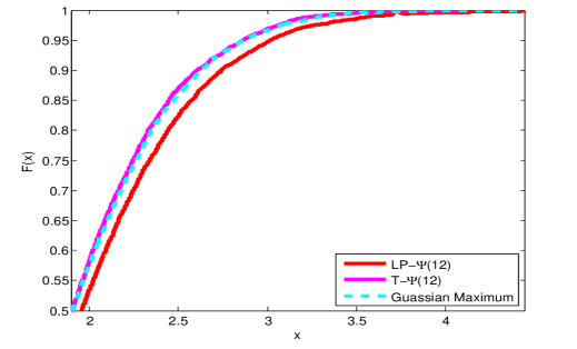
Proposition 7.1 in Section 7 shows that the distribution of the test statistic Ψ^(d)^Ψ𝑑\hat{\Psi}(d) in (2.3) can be consistently estimated by that of the absolute Gaussian maximum |𝐆|subscript𝐆|\mathbf{G}|_{\infty}, where 𝐆=dN(0,𝐈d)subscript𝑑𝐆𝑁0subscript𝐈𝑑\mathbf{G}=_{d}N(0,\mathbf{I}_{d}). To see how close this approximation is, we compare in Figure 1 the cumulative distribution function of |𝐆|subscript𝐆|\mathbf{G}|_{\infty} and the empirical distributions of Ψ^(d)^Ψ𝑑\hat{\Psi}(d) using the trigonometric series (2.7) and the Legendre polynomial (LP) series (2.6), when the data are generated from Student’s t(7)𝑡7t(7)-distribution, with n=180,m=150formulae-sequence𝑛180𝑚150n=180,m=150 and d=12𝑑12d=12. We only present the upper half of the curve since the (1α)1𝛼(1-\alpha) quantile of |𝐆|subscript𝐆|\mathbf{G}|_{\infty} with α(0,1/2)𝛼012\alpha\in(0,1/2) is of particular interest. It can be seen from Figure 1 that the cumulative distribution curves of |𝐆|subscript𝐆|\mathbf{G}|_{\infty} and the trigonometric series based statistic, denoted by T-Ψ^(d)^Ψ𝑑\hat{\Psi}(d), almost coincide, while there is a slightly noticeable difference between |𝐆|subscript𝐆|\mathbf{G}|_{\infty} and the LP polynomial series based statistic LP-Ψ^(d)^Ψ𝑑\hat{\Psi}(d). Indeed, this phenomenon can be expected from the theoretical discoveries. See, for example, the rate of convergence in (7.1) and (7.2), where dependence of {Bd}=0,1,2subscriptsubscript𝐵𝑑012\{B_{\ell d}\}_{\ell=0,1,2} on d𝑑d can be found in (4.2) and (4.3).

Figure 1: Comparison of the empirical cumulative distributions of LP-Ψ^(12)^Ψ12\hat{\Psi}(12), T-Ψ^(12)^Ψ12\hat{\Psi}(12) and the limiting cumulative distribution with n=180𝑛180n=180 and m=150𝑚150m=150. The plot is based on 5000 simulations.
Refer to caption

Next, we carry out 5000 simulations with nominal significance level α=0.05𝛼0.05\alpha=0.05 to calculate the empirical sizes of the proposed smooth test ΦαS(d)superscriptsubscriptΦ𝛼S𝑑\Phi_{\alpha}^{{\rm S}}(d). We denote with T-ΦαS(d)superscriptsubscriptΦ𝛼S𝑑\Phi_{\alpha}^{{\rm S}}(d) and LP-ΦαS(d)superscriptsubscriptΦ𝛼S𝑑\Phi_{\alpha}^{{\rm S}}(d), respectively, the tests based on the trigonometric series (2.7) and the LP polynomial series (2.6). The sample sizes (n,m)𝑛𝑚(n,m) are taken to be (80,60), (120,90), (180,150), and d𝑑d takes values 4,8,1248124,8,12. We compare the proposed smooth test with the testing procedure proposed by Bera, Ghosh and Xiao (2013), the two-sample Kolmogorov-Smirnov test and the two-sample Cramér-von Mises test in five examples when the data are generated from Gamma, Logistic, Gaussian, Pareto and Stable distributions. The results are summarized in Table 1, from which we see that among all the five examples considered, the empirical sizes of T-ΦαS(d)subscriptsuperscriptΦS𝛼𝑑\Phi^{{\rm S}}_{\alpha}(d) with d{4,8,12}𝑑4812d\in\{4,8,12\} are close to 0.05. This highlights the robustness of the testing procedure T-ΦαS(d)subscriptsuperscriptΦS𝛼𝑑\Phi^{{\rm S}}_{\alpha}(d) with respect to the choice of the truncation parameter d𝑑d. Further, we note that the empirical sizes of LP-ΦαS(4)subscriptsuperscriptΦS𝛼4\Phi^{{\rm S}}_{\alpha}(4) are comparable to those of ΦBGXsubscriptΦBGX\Phi_{{\rm BGX}}, while as d𝑑d increases, the test LP-ΦαS(d)subscriptsuperscriptΦS𝛼𝑑\Phi^{{\rm S}}_{\alpha}(d) suffers from size distortion gradually. In fact, as pointed out by Neyman (1937) and Bera and Ghosh (2002), when the Legendre polynomials series is used to construct the test statistic, the effectiveness of the corresponding test in each direction could be diluted if d𝑑d is too large. Nevertheless, the test based on the trigonometric series remains to be efficient as d𝑑d increases and can be very powerful as we shall see later.

Table 1: Comparison of empirical sizes with nominal significance level α=0.05𝛼0.05\alpha=0.05
T-ΦαS(d)T-superscriptsubscriptΦ𝛼S𝑑\text{T-}{\Phi}_{\alpha}^{\text{S}}(d) LP-ΦαS(d)LP-superscriptsubscriptΦ𝛼S𝑑\text{LP-}{\Phi}_{\alpha}^{\text{S}}(d) BGX KS CVM
Model (n,m)𝑛𝑚(n,m) d=4𝑑4d=4 d=8𝑑8d=8 d=12𝑑12d=12 d=4𝑑4d=4 d=8𝑑8d=8 d=12𝑑12d=12
Gamma(2,2) (80,60)8060(80,60) 0.0504 0.0500 0.0490 0.0584 0.0724 0.1078 0.0634 0.0494 0.0524
(120,90)12090(120,90) 0.0504 0.0510 0.0484 0.0542 0.0654 0.0830 0.0590 0.0438 0.0434
(180,150)180150(180,150) 0.0496 0.0486 0.0484 0.0500 0.0554 0.0706 0.0530 0.0440 0.0444
Logistic(0,1) (80,60)8060(80,60) 0.0498 0.0496 0.0482 0.0576 0.0748 0.1038 0.0618 0.0456 0.0494
(120,90)12090(120,90) 0.0504 0.0500 0.0496 0.0528 0.0666 0.0860 0.0552 0.0504 0.0466
(180,150)180150(180,150) 0.0502 0.0498 0.0500 0.0508 0.0570 0.0696 0.0574 0.0438 0.0424
N(0,1) (80,60)8060(80,60) 0.0504 0.0488 0.0470 0.0570 0.0764 0.1060 0.0648 0.0494 0.0504
(120,90)12090(120,90) 0.0502 0.0494 0.0482 0.0548 0.0694 0.0850 0.0566 0.053 0.0504
(180,150)180150(180,150) 0.0502 0.0514 0.0516 0.0504 0.0544 0.0616 0.0542 0.0446 0.0500
Pareto(0.5,1,1) (80,60)8060(80,60) 0.0502 0.0484 0.0468 0.0582 0.0766 0.1064 0.0640 0.0460 0.0494
(120,90)12090(120,90) 0.0500 0.0494 0.0494 0.0540 0.0640 0.0824 0.0592 0.0468 0.0480
(180,150)180150(180,150) 0.0498 0.0496 0.0500 0.0530 0.0586 0.0724 0.0542 0.0436 0.0456
Stable(1.5,0,1,1) (80,60)8060(80,60) 0.0480 0.0470 0.0456 0.0544 0.0758 0.1088 0.0606 0.0474 0.0488
(120,90)12090(120,90) 0.0496 0.0498 0.0494 0.0578 0.0692 0.0790 0.0614 0.0492 0.0514
(180,150)180150(180,150) 0.0510 0.0514 0.0506 0.0508 0.0570 0.0690 0.0608 0.0490 0.0484

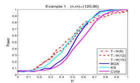
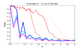
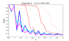
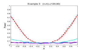
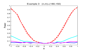
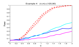
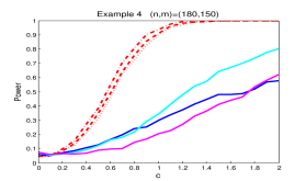
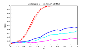
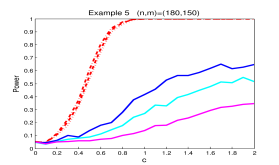
The power performance is evaluated through the following five examples. In each example, the result reported is based on 1000 simulations where samples sizes (n,m)𝑛𝑚(n,m) are taken to be (120,90)12090(120,90) and (180,150)180150(180,150). Because of the distortion of empirical sizes of LP-ΦαS(d)superscriptsubscriptΦ𝛼S𝑑\Phi_{\alpha}^{{\rm S}}(d), we only compare the power of the trigonometric series based smooth test T-ΦαS(d)superscriptsubscriptΦ𝛼S𝑑\Phi_{\alpha}^{{\rm S}}(d) with that of the KS, CVM and BGX tests. The plots of power functions against different families of alternative distributions from Examples 15 are given in Figure 2.

Example 1.
X:F=uniform(1,1)versus:𝑋𝐹uniform11versus\displaystyle X:F=\text{uniform}\,(-1,1)\ \ \mbox{versus }
Y:G=Gμ with density gμ(x)=12+2xμ|x|μ2I(|x|<μ)(0μ1).:𝑌formulae-sequence𝐺subscript𝐺𝜇 with density subscript𝑔𝜇𝑥122𝑥𝜇𝑥superscript𝜇2𝐼𝑥𝜇0𝜇1\displaystyle Y:G=G_{\mu}\ \ \mbox{ with density }\ \ g_{\mu}(x)=\frac{1}{2}+2x\frac{\mu-|x|}{\mu^{2}}I(|x|<\mu)\quad(0\leq\mu\leq 1).
Example 2.
X:F=uniform(1,1) versus:𝑋𝐹uniform11 versus\displaystyle X:F=\text{uniform}\,(-1,1)\ \ \mbox{ versus}
Y:G=Gσ with density gσ(x)=12{1+sin(2πσx)}(0.5σ5).:𝑌formulae-sequence𝐺subscript𝐺𝜎 with density subscript𝑔𝜎𝑥1212𝜋𝜎𝑥0.5𝜎5\displaystyle Y:G=G_{\sigma}\ \ \mbox{ with density }\ \ g_{\sigma}(x)=\frac{1}{2}\{1+\sin(2\pi\sigma x)\}\quad(0.5\leq\sigma\leq 5).
Example 3.
X:F=lognormal(0,1) with densityf(x)=(2π)1/2x1exp{(logx)2/2} versus:𝑋formulae-sequence𝐹lognormal01 with density𝑓𝑥superscript2𝜋12superscript𝑥1superscript𝑥22 versus\displaystyle X:F=\text{lognormal}\,(0,1)\ \ \mbox{ with density}\ \ f(x)=(2\pi)^{-1/2}x^{-1}\exp\{-(\log x)^{2}/2\}\ \ \mbox{ versus }
Y:G=Ga with densityga(x)=f(x){1+asin(2πlogx)}(1a1).:𝑌formulae-sequence𝐺subscript𝐺𝑎 with densitysubscript𝑔𝑎𝑥𝑓𝑥1𝑎2𝜋𝑥1𝑎1\displaystyle Y:G=G_{a}\ \ \mbox{ with density}\ \ g_{a}(x)=f(x)\{1+a\sin(2\pi\log x)\}\ \ (-1\leq a\leq 1).
Example 4.
X:F=uniform(0,1) versus:𝑋𝐹uniform01 versus\displaystyle X:F=\text{uniform}\,(0,1)\ \ \mbox{ versus }
Y:G=Gc with density gc(x)=exp{csin(5πx)}(0c2).:𝑌formulae-sequence𝐺subscript𝐺𝑐 with density subscript𝑔𝑐𝑥𝑐5𝜋𝑥0𝑐2\displaystyle Y:G=G_{c}\ \ \mbox{ with density }\ \ g_{c}(x)=\exp\{c\sin(5\pi x)\}\ \ (0\leq c\leq 2).
Example 5.
X:F=uniform(0,1) versus:𝑋𝐹uniform01 versus\displaystyle X:F=\text{uniform}\,(0,1)\ \ \mbox{ versus }
Y:G=Gc with density gc(x)=1+ccos(5πx)(0c2).:𝑌formulae-sequence𝐺subscript𝐺𝑐 with density subscript𝑔𝑐𝑥1𝑐5𝜋𝑥0𝑐2\displaystyle Y:G=G_{c}\ \ \mbox{ with density }\ \ g_{c}(x)=1+c\cos(5\pi x)\ \ (0\leq c\leq 2).

The first two examples are, respectively, Examples 5 and 6 in Fan (1996) which were designed to demonstrate the performance of the adaptive Neyman’s test proposed there. In Example 1, when μ=0𝜇0\mu=0, Gμsubscript𝐺𝜇G_{\mu} coincides with F𝐹F. For this family of alternatives index by μ𝜇\mu, the strength of the local feature depends on μ𝜇\mu in the sense that the larger the μ𝜇\mu, the stronger the local feature. As expected, the powers of all the tests considered grow with μ𝜇\mu and when sample sizes are large enough, the smooth tests T-ΦαS(d)subscriptsuperscriptΦS𝛼𝑑\Phi^{{\rm S}}_{\alpha}(d) uniformly outperform the others. Example 2, on the other hand, is designed to test the global features with various frequencies. It can be seen from the second row in Figure 2 that the test T-ΦαS(16)subscriptsuperscriptΦS𝛼16\Phi^{{\rm S}}_{\alpha}(16) has the highest power that approaches to 1 rapidly as σ𝜎\sigma decreases to 0. The third example is from Heyde (1963), where gasubscript𝑔𝑎g_{a} is a density and has the same moments as f0subscript𝑓0f_{0} of any order. In this example, all the KS, CVM and BGX tests suffer from very poor power, while surprisingly, the smooth tests based on the trigonometric series remain powerful. The last two examples aim to cover the high-frequency alternations. Again, the proposed tests have the highest powers. In fact, the BGX test was originally constructed to identify deviations in the directions of mean, variance, skewness and kurtosis, and hence it can be relatively less powerful in detecting local features or high-frequency components.

Figure 2: Empirical powers for Examples 15 based on 1000 replications with α=0.05𝛼0.05\alpha=0.05
Refer to caption Refer to caption

5.2 Multivariate case

The computation of the proposed multivariate smooth test and the critical value requires to find optimal directions u^maxsubscript^𝑢\hat{u}_{\max} and u^maxMBsuperscriptsubscript^𝑢MB\hat{u}_{\max}^{{\rm MB}} on the unit sphere 𝒮p1superscript𝒮𝑝1\mathcal{S}^{p-1} that maximize non-smooth objective functions (3.3) and (3.6), respectively. To solve these optimization problems, we convert the data into spherical coordinates and employ the Nelder-Mead algorithm. As a trade-off between the power and the computational feasibility of the test, we keep the value of d𝑑d fixed at 4.

Similar to the univariate case, we first carry out 5000 simulations with nominal significance level α=0.05𝛼0.05\alpha=0.05 to calculate the empirical sizes of the proposed test T-ΦαMS(d)superscriptsubscriptΦ𝛼MS𝑑\Phi_{\alpha}^{{\rm MS}}(d) with trigonometric series. For each p{3,5,10}𝑝3510p\in\{3,5,10\}, the data are generated from multivariate normal and t𝑡t-distributions with different degrees of freedom (444 and 888) and covariance structures (Ipsubscript𝐼𝑝I_{p} and ΣΣ\Sigma). Sample sizes (n,m)𝑛𝑚(n,m) are taken to be (180,160). We summarize the results in Table 2, comparing with the method proposed by Baringhaus and Franz (2004), which will be referred as the BF test. From Table 2 we see that when p=3,5𝑝35p=3,5, both methods have an empirical size fairly close to 0.05; when p=10𝑝10p=10, the empirical size of the proposed smooth test increases since the optimization over the unit sphere becomes more challenging, while the empirical size of the BF test is typically smaller than the nominal level.

Table 2: Empirical size with significance level α=0.05𝛼0.05\alpha=0.05.
Multivariate Normal Multivariate t
N(0,Ip)𝑁0subscript𝐼𝑝N(0,I_{p}) N(0,Σ)𝑁0ΣN(0,\Sigma) t4(0,Ip)subscript𝑡40subscript𝐼𝑝t_{4}(0,I_{p}) t8(0,Ip)subscript𝑡80subscript𝐼𝑝t_{8}(0,I_{p}) t4(0,Σ)subscript𝑡40Σt_{4}(0,\Sigma) t8(0,Σ)subscript𝑡80Σt_{8}(0,\Sigma)
p=3𝑝3p=3 T-ΦαMS(d)T-superscriptsubscriptΦ𝛼MS𝑑\text{T-}{\Phi}_{\alpha}^{\text{MS}}(d) 0.04460.04460.0446 0.04560.04560.0456 0.05140.05140.0514 0.04420.04420.0442 0.04940.04940.0494 0.04580.04580.0458
BF 0.04800.04800.0480 0.04940.04940.0494 0.05040.05040.0504 0.04880.04880.0488 0.04480.04480.0448 0.04840.04840.0484
p=5𝑝5p=5 T-ΦαMS(d)T-superscriptsubscriptΦ𝛼MS𝑑\text{T-}{\Phi}_{\alpha}^{\text{MS}}(d) 0.04960.04960.0496 0.04720.04720.0472 0.04940.04940.0494 0.05600.05600.0560 0.04500.04500.0450 0.05140.05140.0514
BF 0.04660.04660.0466 0.04720.04720.0472 0.05020.05020.0502 0.04580.04580.0458 0.04880.04880.0488 0.04840.04840.0484
p=10𝑝10p=10 T-ΦαMS(d)T-superscriptsubscriptΦ𝛼MS𝑑\text{T-}{\Phi}_{\alpha}^{\text{MS}}(d) 0.05820.05820.0582 0.05940.05940.0594 0.05120.05120.0512 0.05160.05160.0516 0.05700.05700.0570 0.06020.06020.0602
BF 0.04220.04220.0422 0.04540.04540.0454 0.03640.03640.0364 0.04220.04220.0422 0.04820.04820.0482 0.04380.04380.0438

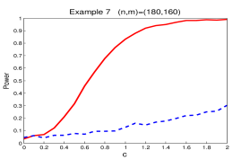
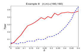
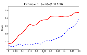
The power performance of the multivariate smooth test is evaluated through Examples 69. The first two are multivariate versions of Examples 1 and 4, which demonstrate, respectively, the alternations with local feature and high frequency. The last two examples are designed to examine a rotation effect in the alternations. In each one, the power reported is based on 1000 simulations where samples sizes (n,m)𝑛𝑚(n,m) are taken to be (180,160)180160(180,160). Again, we compare the power of the trigonometric series based smooth test T-ΦαS(d)superscriptsubscriptΦ𝛼S𝑑\Phi_{\alpha}^{{\rm S}}(d) with that of the BF test. The power curve are depicted in Figure 3.

Example 6.
X=(X1,X2,X3),X1,X2iiduniform(1,1),X3=0.3X1+0.7X2versusformulae-sequence𝑋superscriptsubscript𝑋1subscript𝑋2subscript𝑋3subscript𝑋1subscript𝑋2𝑖𝑖𝑑similar-touniform11subscript𝑋30.3subscript𝑋10.7subscript𝑋2versus\displaystyle X=(X_{1},X_{2},X_{3})^{\intercal},\ \ X_{1},X_{2}\overset{iid}{\sim}\text{uniform}\,(-1,1),\ \ X_{3}=0.3X_{1}+0.7X_{2}\ \ \mbox{versus}
Y=(Y1,Y2,Y3),Y1,Y2iidgμ(x)=12+2xμ|x|μ2I(|x|<μ)(0μ1)formulae-sequence𝑌superscriptsubscript𝑌1subscript𝑌2subscript𝑌3subscript𝑌1subscript𝑌2𝑖𝑖𝑑similar-tosubscript𝑔𝜇𝑥122𝑥𝜇𝑥superscript𝜇2𝐼𝑥𝜇0𝜇1\displaystyle Y=(Y_{1},Y_{2},Y_{3})^{\intercal},\ \ Y_{1},Y_{2}\overset{iid}{\sim}g_{\mu}(x)=\frac{1}{2}+2x\frac{\mu-|x|}{\mu^{2}}I(|x|<\mu)\,(0\leq\mu\leq 1)
Y3=0.3Y1+0.7Y2.subscript𝑌30.3subscript𝑌10.7subscript𝑌2\displaystyle Y_{3}=0.3Y_{1}+0.7Y_{2}.
Example 7.
X=(X1,X2,X3),X1,X2iiduniform(0,1),X3=0.3X1+0.7X2versusformulae-sequence𝑋superscriptsubscript𝑋1subscript𝑋2subscript𝑋3subscript𝑋1subscript𝑋2𝑖𝑖𝑑similar-touniform01subscript𝑋30.3subscript𝑋10.7subscript𝑋2versus\displaystyle X=(X_{1},X_{2},X_{3})^{\intercal},\ \ X_{1},X_{2}\overset{iid}{\sim}\text{uniform}\,(0,1),\ \ X_{3}=0.3X_{1}+0.7X_{2}\ \ \mbox{versus}
Y=(Y1,Y2,Y3),Y1,Y2iidgc(x)=exp{csin(5πx)}(0c2),Y3=0.3Y1+0.7Y2.formulae-sequence𝑌superscriptsubscript𝑌1subscript𝑌2subscript𝑌3subscript𝑌1formulae-sequencesubscript𝑌2𝑖𝑖𝑑similar-tosubscript𝑔𝑐𝑥𝑐5𝜋𝑥0𝑐2subscript𝑌30.3subscript𝑌10.7subscript𝑌2\displaystyle Y=(Y_{1},Y_{2},Y_{3})^{\intercal},\ \ Y_{1},Y_{2}\overset{iid}{\sim}g_{c}(x)=\exp\{c\sin(5\pi x)\}\,(0\leq c\leq 2),\,Y_{3}=0.3Y_{1}+0.7Y_{2}.
Example 8.
X𝒩(0,I5)versusY=AZ,Z𝒩(0,I5),formulae-sequencesimilar-to𝑋𝒩0subscript𝐼5versusformulae-sequence𝑌𝐴𝑍similar-to𝑍𝒩0subscript𝐼5\displaystyle X\sim\mathcal{N}(0,I_{5})\ \ \mbox{versus}\ \ Y=AZ,\ \ Z\sim\mathcal{N}(0,I_{5}),
where A=(A000I3),A0=(1δδδ1δ)(0δ0.5).formulae-sequencewhere 𝐴subscript𝐴000subscript𝐼3subscript𝐴01𝛿𝛿𝛿1𝛿0𝛿0.5\displaystyle\mbox{ where }A=\left(\begin{array}[]{cc}A_{0}&0\\ 0&I_{3}\end{array}\right),\ \ A_{0}=\left(\begin{array}[]{cc}\sqrt{1-\delta}&\sqrt{\delta}\\ \sqrt{\delta}&\sqrt{1-\delta}\end{array}\right)\,(0\leq\delta\leq 0.5).
Example 9.
Xt4(0,I5)versusY=AZ,Zt4(0,I5),formulae-sequencesimilar-to𝑋subscript𝑡40subscript𝐼5versusformulae-sequence𝑌𝐴𝑍similar-to𝑍subscript𝑡40subscript𝐼5\displaystyle X\sim t_{4}(0,I_{5})\ \ \mbox{versus}\ \ Y=AZ,\quad Z\sim t_{4}(0,I_{5}),
where A=(A000I3),A0=(1δδδ1δ)(0δ0.5).formulae-sequencewhere 𝐴subscript𝐴000subscript𝐼3subscript𝐴01𝛿𝛿𝛿1𝛿0𝛿0.5\displaystyle\mbox{ where }A=\left(\begin{array}[]{cc}A_{0}&0\\ 0&I_{3}\end{array}\right),\ \ A_{0}=\left(\begin{array}[]{cc}\sqrt{1-\delta}&\sqrt{\delta}\\ \sqrt{\delta}&\sqrt{1-\delta}\end{array}\right)\,(0\leq\delta\leq 0.5).
Figure 3: Empirical powers for Examples 69 based on 1000 replications with α=0.05𝛼0.05\alpha=0.05
Refer to caption Refer to caption

Figure 3 shows that the proposed smooth test uniformly outperforms the BF test in all the examples in terms of power. Since we are using trigonometric series, the test is powerful especially if the data contains high frequency components (Example 7), which is difficult to be detected by the BF test.

6 Discussion

We introduced in this paper a smooth test for the equality of two unknown distributions, which is shown to maintain the pre-specified significance level asymptotically. Moreover, it was shown theoretically and numerically that the test is especially powerful in detecting local features or high-frequency components.

The proposed procedure depends on a user-specific parameter d𝑑d, which is the number of orthogonal directions used to construct the test statistic. Theoretically, the size of d𝑑d is allowed to grow with n𝑛n and can be as large as o(nc)𝑜superscript𝑛𝑐o(n^{c}) for some 0<c<10𝑐10<c<1. Since the optimal value of d𝑑d depends on how far the two unknown distributions deviate from each other, it is not possible to practically define an optimal choice of d𝑑d. As suggested by our numerical studies, d=10𝑑10d=10 is a reasonable choice when the sample sizes are in the order of 102superscript10210^{2}, which leads a good compromise between the computational cost and the performance of the test. Alternatively, a data-driven approach based on a modification of Schwarz’s rule was proposed by Inglot, Kallenberg and Ledwina (1997), that is, d^=argmax1dD(n,m){T(d)dlog(n+m)}^𝑑subscriptarg1𝑑𝐷𝑛𝑚𝑇𝑑𝑑𝑛𝑚\hat{d}=\mathop{\rm arg\max}_{1\leq d\leq D(n,m)}\{T(d)-d\log(n+m)\} for some D(n,m)𝐷𝑛𝑚D(n,m)\rightarrow\infty as min(n,m)𝑛𝑚\min(n,m)\to\infty, where T(d)𝑇𝑑T(d) is the test statistic using the first d𝑑d orthonormal functions. This principal can be applied to the proposed testing procedure by setting D(n,m)𝐷𝑛𝑚D(n,m) to be some large value, say 202020. Nevertheless, the optimal choice of D(n,m)𝐷𝑛𝑚D(n,m) remains unclear.

The computation of the multivariate test statistic Ψ^max(d)subscript^Ψ𝑑\hat{\Psi}_{\max}(d) requires solving the optimization problem with an 2subscript2\ell_{2}-norm constraint. To solve this problem when the dimension p𝑝p is relatively small, we first convert the data into spherical coordinates and then use the Nelder-Mead algorithm. An interesting extension is to combine our method with the smoothing technique as in Horowitz (1992). Let K::𝐾maps-toK:\mathbb{R}\mapsto\mathbb{R} be a symmetric, bounded density function. For a predetermined small number h=hn>0subscript𝑛0h=h_{n}>0, ψ^u,ksubscript^𝜓𝑢𝑘\hat{\psi}_{u,k} is approximated by a continuous function ψ^u,k,h=m1j=1mψk(V^j,hu)subscript^𝜓𝑢𝑘superscript𝑚1superscriptsubscript𝑗1𝑚subscript𝜓𝑘subscriptsuperscript^𝑉𝑢𝑗\hat{\psi}_{u,k,h}=m^{-1}\sum_{j=1}^{m}\psi_{k}(\hat{V}^{u}_{j,h}), where

V^j,hu=1ni=1n𝒦{u(YjXi)h} with 𝒦(t)=tK(z)𝑑z.formulae-sequencesubscriptsuperscript^𝑉𝑢𝑗1𝑛superscriptsubscript𝑖1𝑛𝒦superscript𝑢subscript𝑌𝑗subscript𝑋𝑖 with 𝒦𝑡superscriptsubscript𝑡𝐾𝑧differential-d𝑧\hat{V}^{u}_{j,h}=\frac{1}{n}\sum_{i=1}^{n}\mathcal{K}\bigg{\{}\frac{u^{\intercal}(Y_{j}-X_{i})}{h}\bigg{\}}\ \ \mbox{ with }\ \ \mathcal{K}(t)=\int_{-\infty}^{t}K(z)\,dz.

As h00h\rightarrow 0, V^j,husubscriptsuperscript^𝑉𝑢𝑗\hat{V}^{u}_{j,h} converges to V^jusubscriptsuperscript^𝑉𝑢𝑗\hat{V}^{u}_{j} almost surely, and hence for each k[d]𝑘delimited-[]𝑑k\in[d], supu𝒮p1|ψ^k,u,h|subscriptsupremum𝑢superscript𝒮𝑝1subscript^𝜓𝑘𝑢\sup_{u\in\mathcal{S}^{p-1}}|\hat{\psi}_{k,u,h}| is a smoothed version of supu𝒮p1|ψ^u,k|subscriptsupremum𝑢superscript𝒮𝑝1subscript^𝜓𝑢𝑘\sup_{u\in\mathcal{S}^{p-1}}|\hat{\psi}_{u,k}|. The smoothing technique can be similarly applied to the multiplier bootstrap statistic. Consequently, we can employ the gradient descent algorithm to solve the optimization for smooth functions. We leave a thorough comparison of various algorithms for different values of p𝑝p as an interesting problem for future research.

7 Proof of the main results

In this section we prove Theorems 4.14.3. Proofs of the lemmas and some additional technical arguments are given in the Appendix. Throughout this section, we write N=n+m𝑁𝑛𝑚N=n+m and use C𝐶C and c𝑐c to denote absolute positive constants, which may take different values at each occurrence. We write abless-than-or-similar-to𝑎𝑏a\lesssim b if a𝑎a is smaller than or equal to b𝑏b up to an absolute positive constant, and abgreater-than-or-equivalent-to𝑎𝑏a\gtrsim b if baless-than-or-similar-to𝑏𝑎b\lesssim a.

7.1 Proof of Theorem 4.1

Recall that 𝐆=(G1,,Gd)𝐆superscriptsubscript𝐺1subscript𝐺𝑑\mathbf{G}=(G_{1},\ldots,G_{d})^{\intercal} is a d𝑑d-dimensional standard Gaussian random vector, the distribution of |𝐆|subscript𝐆|\mathbf{G}|_{\infty} is absolute continuous so that P{|𝐆|cα(d)}=α𝑃subscript𝐆subscript𝑐𝛼𝑑𝛼P\{|\mathbf{G}|_{\infty}\geq c_{\alpha}(d)\}=\alpha. Therefore, under the assumption that dnm𝑑𝑛𝑚d\leq n\wedge m, the conclusion (4.8) follows from the following proposition immediately.

Proposition 7.1.

Assume that the conditions of Theorem 4.1 hold and let

γ0n=(logn)7/8n1/8B0d,γ1n=(logd)3/2nB1d,γ2n=logdnB2d.formulae-sequencesubscript𝛾0𝑛superscript𝑛78superscript𝑛18subscript𝐵0𝑑formulae-sequencesubscript𝛾1𝑛superscript𝑑32𝑛subscript𝐵1𝑑subscript𝛾2𝑛𝑑𝑛subscript𝐵2𝑑\gamma_{0n}=\frac{(\log n)^{7/8}}{n^{1/8}}B_{0d},\ \ \gamma_{1n}=\frac{(\log d)^{3/2}}{\sqrt{n}}B_{1d},\ \ \gamma_{2n}=\sqrt{\frac{\log d}{n}}B_{2d}. (7.1)

Then under H0:F=G:subscript𝐻0𝐹𝐺H_{0}:F=G,

supt0|P{Ψ^(d)t}P(|𝐆|t)|γ0n+γ1n+γ2n.less-than-or-similar-tosubscriptsupremum𝑡0𝑃^Ψ𝑑𝑡𝑃subscript𝐆𝑡subscript𝛾0𝑛subscript𝛾1𝑛subscript𝛾2𝑛\displaystyle\sup_{t\geq 0}\big{|}P\big{\{}\hat{\Psi}(d)\leq t\big{\}}-P\big{(}|\mathbf{G}|_{\infty}\leq t\big{)}\big{|}\lesssim\gamma_{0n}+\sqrt{\gamma_{1n}}+\sqrt{\gamma_{2n}}. (7.2)

The proof of Proposition 7.1 is provided in Section 7.4.1. ∎

7.2 Proof of Theorem 4.2

For the d𝑑d-dimensional Gaussian random vector 𝐆𝐆\mathbf{G}, applying the Borell-TIS (Borell-Tsirelson-Ibragimov-Sudakov) inequality (van der Vaart and Wellner, 1996) yields that for every t>0𝑡0t>0, P{|𝐆|>E(|𝐆|)+t}exp(t2/2)𝑃subscript𝐆𝐸subscript𝐆𝑡superscript𝑡22P\{|\mathbf{G}|_{\infty}>E(|\mathbf{G}|_{\infty})+t\}\leq\exp(-t^{2}/2). By taking t=2log(1/α)𝑡21𝛼t=\sqrt{2\log(1/\alpha)}, we get

cα(d)E(|𝐆|)+2log(1/α),subscript𝑐𝛼𝑑𝐸subscript𝐆21𝛼c_{\alpha}(d)\leq E(|\mathbf{G}|_{\infty})+\sqrt{2\log(1/\alpha)}, (7.3)

where cα(d)subscript𝑐𝛼𝑑c_{\alpha}(d) denotes the (1α)1𝛼(1-\alpha)-quantile of |𝐆|subscript𝐆|\mathbf{G}|_{\infty}. A standard result on Gaussian maxima yields E(|𝐆|){1+(2logd)1}2logd𝐸subscript𝐆1superscript2𝑑12𝑑E(|\mathbf{G}|_{\infty})\leq\{1+(2\log d)^{-1}\}\sqrt{2\log d}.

Let k=argmaxk[d]|θk|superscript𝑘subscript𝑘delimited-[]𝑑subscript𝜃𝑘k^{*}=\arg\max_{k\in[d]}|\theta_{k}| under H1dsubscriptsuperscript𝐻𝑑1H^{d}_{1} and assume without loss of generality that θk>0subscript𝜃superscript𝑘0\theta_{k^{*}}>0. By (7.7) and (7.10) in the proof of Proposition 7.1, we have

PH1d{Ψ^>cα(d)}subscript𝑃subscriptsuperscript𝐻𝑑1^Ψsubscript𝑐𝛼𝑑\displaystyle P_{H^{d}_{1}}\big{\{}\hat{\Psi}>c_{\alpha}(d)\big{\}} PH1d{nmNψ^k>cα(d)}absentsubscript𝑃subscriptsuperscript𝐻𝑑1𝑛𝑚𝑁subscript^𝜓superscript𝑘subscript𝑐𝛼𝑑\displaystyle\geq P_{H^{d}_{1}}\bigg{\{}\sqrt{\frac{nm}{N}}\,\hat{\psi}_{k^{*}}>c_{\alpha}(d)\bigg{\}}
=PH1d{1Nj=1Nξjk+nmN(R1k+R2k)>cα(d)},absentsubscript𝑃subscriptsuperscript𝐻𝑑11𝑁superscriptsubscript𝑗1𝑁subscript𝜉𝑗superscript𝑘𝑛𝑚𝑁subscript𝑅1superscript𝑘subscript𝑅2superscript𝑘subscript𝑐𝛼𝑑\displaystyle=P_{H^{d}_{1}}\bigg{\{}\frac{1}{\sqrt{N}}\sum_{j=1}^{N}\xi_{jk^{*}}+\sqrt{\frac{nm}{N}}(R_{1k^{*}}+R_{2k^{*}})>c_{\alpha}(d)\bigg{\}}, (7.4)

where ξjk=n/m{ψk(Vj)ϑk}I{j[m]}+m/nh1k(Xjm)I{jm+[n]}subscript𝜉𝑗𝑘𝑛𝑚subscript𝜓𝑘subscript𝑉𝑗subscriptitalic-ϑ𝑘𝐼𝑗delimited-[]𝑚𝑚𝑛subscript1𝑘subscript𝑋𝑗𝑚𝐼𝑗𝑚delimited-[]𝑛\xi_{jk}=\sqrt{n/m}\,\{\psi_{k}(V_{j})-\vartheta_{k}\}I\{j\in[m]\}+\sqrt{m/n}\,h_{1k}(X_{j-m})I\{j\in m+[n]\} for (j,k)[N]×[d]𝑗𝑘delimited-[]𝑁delimited-[]𝑑(j,k)\in[N]\times[d] with Vj=F(Yj)subscript𝑉𝑗𝐹subscript𝑌𝑗V_{j}=F(Y_{j}), ϑk=EH1d{ψk(V)}subscriptitalic-ϑ𝑘subscript𝐸subscriptsuperscript𝐻𝑑1subscript𝜓𝑘𝑉\vartheta_{k}=E_{H^{d}_{1}}\{\psi_{k}(V)\} and h1k(x)=EH1d(ψk(V)[I{VF(x)}V])subscript1𝑘𝑥subscript𝐸subscriptsuperscript𝐻𝑑1subscriptsuperscript𝜓𝑘𝑉delimited-[]𝐼𝑉𝐹𝑥𝑉h_{1k}(x)=E_{H^{d}_{1}}(\psi^{\prime}_{k}(V)[I\{V\geq F(x)\}-V]). Note that E{h1k(X)}=0𝐸subscript1𝑘𝑋0E\{h_{1k}(X)\}=0 and thus E(ξjk)=0𝐸subscript𝜉𝑗𝑘0E(\xi_{jk})=0. Let (t1,t2)subscript𝑡1subscript𝑡2\mathcal{E}(t_{1},t_{2}) be as in (7.12) for t1,t2>0subscript𝑡1subscript𝑡20t_{1},t_{2}>0 to be specified. Put δ=t1B2d+t2B1d+nm/N(θkϑk)+2log(1/α)𝛿subscript𝑡1subscript𝐵2𝑑subscript𝑡2subscript𝐵1𝑑𝑛𝑚𝑁subscript𝜃superscript𝑘subscriptitalic-ϑsuperscript𝑘21𝛼\delta=t_{1}B_{2d}+t_{2}B_{1d}+\sqrt{nm/N}(\theta_{k^{*}}-\vartheta_{k^{*}})+\sqrt{2\log(1/\alpha)}, then it follows from (7.3) and (7.4) that

PH1d{Ψ^>cα(d)}subscript𝑃subscriptsuperscript𝐻𝑑1^Ψsubscript𝑐𝛼𝑑\displaystyle P_{H^{d}_{1}}\big{\{}\hat{\Psi}>c_{\alpha}(d)\big{\}}
PH1d{1Nj=1Nξjk>(1+12logd)2logd+δnmNθk}P{(t1,t2)c}absentsubscript𝑃subscriptsuperscript𝐻𝑑11𝑁superscriptsubscript𝑗1𝑁subscript𝜉𝑗superscript𝑘112𝑑2𝑑𝛿𝑛𝑚𝑁subscript𝜃superscript𝑘𝑃superscriptsubscript𝑡1subscript𝑡2c\displaystyle\geq P_{H^{d}_{1}}\bigg{\{}\frac{1}{\sqrt{N}}\sum_{j=1}^{N}\xi_{jk^{*}}>\bigg{(}1+\frac{1}{2\log d}\bigg{)}\sqrt{2\log d}+\delta-\sqrt{\frac{nm}{N}}\,\theta_{k^{*}}\bigg{\}}-P\big{\{}\mathcal{E}(t_{1},t_{2})^{{\rm c}}\big{\}}
PH1d{1Nj=1Nξjk>(12logdε2)2logd+δ}P{(t1,t2)c}.absentsubscript𝑃subscriptsuperscript𝐻𝑑11𝑁superscriptsubscript𝑗1𝑁subscript𝜉𝑗superscript𝑘12𝑑𝜀22𝑑𝛿𝑃superscriptsubscript𝑡1subscript𝑡2c\displaystyle\geq P_{H^{d}_{1}}\bigg{\{}\frac{1}{\sqrt{N}}\sum_{j=1}^{N}\xi_{jk^{*}}>\bigg{(}\frac{1}{2\log d}-\frac{\varepsilon}{2}\bigg{)}\sqrt{2\log d}+\delta\bigg{\}}-P\big{\{}\mathcal{E}(t_{1},t_{2})^{{\rm c}}\big{\}}.

In particular, taking t1=t1n(d)n1/2logdsubscript𝑡1subscript𝑡1𝑛𝑑asymptotically-equalssuperscript𝑛12𝑑t_{1}=t_{1n}(d)\asymp n^{-1/2}\sqrt{\log d} and t2=t2n(d)n1/2logdsubscript𝑡2subscript𝑡2𝑛𝑑asymptotically-equalssuperscript𝑛12𝑑t_{2}=t_{2n}(d)\asymp n^{-1/2}\log d implies by (7.16) that P{(t1,t2)c}0𝑃superscriptsubscript𝑡1subscript𝑡2c0P\{\mathcal{E}(t_{1},t_{2})^{{\rm c}}\}\rightarrow 0 as d𝑑d\rightarrow\infty. Further, by (8.8) and the conditions of the theorem, we have δ=o(logd)𝛿𝑜𝑑\delta=o(\sqrt{\log d}). Consequently, as d𝑑d\rightarrow\infty,

PH1d{Ψ^>cα(d)}1PH1d(1Nj=1Nξjkε2logd)P{(t1,t2)c}1.subscript𝑃subscriptsuperscript𝐻𝑑1^Ψsubscript𝑐𝛼𝑑1subscript𝑃subscriptsuperscript𝐻𝑑11𝑁superscriptsubscript𝑗1𝑁subscript𝜉𝑗superscript𝑘𝜀2𝑑𝑃superscriptsubscript𝑡1subscript𝑡2c1\displaystyle P_{H^{d}_{1}}\big{\{}\hat{\Psi}>c_{\alpha}(d)\big{\}}\geq 1-P_{H^{d}_{1}}\bigg{(}\frac{1}{\sqrt{N}}\sum_{j=1}^{N}\xi_{jk^{*}}\leq-\frac{\varepsilon}{2}\sqrt{\log d}\bigg{)}-P\big{\{}\mathcal{E}(t_{1},t_{2})^{{\rm c}}\big{\}}\rightarrow 1.

This completes the proof of Theorem 4.2. ∎

7.3 Proof of Theorem 4.3

We first introduce two propositions describing the limiting null properties of the multivariate smooth and multiplier bootstrap statistics used to construct the test. The conclusion of Theorem 4.3 follows immediately.

The first proposition characterizes the non-asymptotic behavior of the multivariate smooth statistic Ψ^max(d)subscript^Ψ𝑑\hat{\Psi}_{\max}(d) which involves the supremum of a centered Gaussian process. Let =dpsubscriptsuperscript𝑝𝑑{\mathcal{F}}={\mathcal{F}}^{p}_{d} be as in (3.4) and for simplicity, the dependence of {\mathcal{F}} on (p,d)𝑝𝑑(p,d) will be assumed without displaying.

Proposition 7.2.

Suppose that Assumptions 4.1 and 4.3 hold. Then there exists a centered, tight Gaussian process 𝔾𝔾\mathbb{G} indexed by {\mathcal{F}} such that under the null hypothesis H0:F=G:subscript𝐻0𝐹𝐺H_{0}:F=G,

supt0|P{Ψ^max(d)t}P(𝔾t)|Cnc,subscriptsupremum𝑡0𝑃subscript^Ψ𝑑𝑡𝑃subscriptnorm𝔾𝑡𝐶superscript𝑛𝑐\displaystyle\sup_{t\geq 0}\big{|}P\big{\{}\hat{\Psi}_{\max}(d)\leq t\big{\}}-P\big{(}\|\mathbb{G}\|_{{\mathcal{F}}}\leq t\big{)}\big{|}\leq C\,n^{-c}, (7.5)

where C𝐶C and c𝑐c are positive constants depending only on c0,c1,C0subscript𝑐0subscript𝑐1subscript𝐶0c_{0},c_{1},C_{0} and C1subscript𝐶1C_{1}.

Proposition 7.2 implies that the “limiting” distribution of Ψ^maxsubscript^Ψ\hat{\Psi}_{\max} depends on unknown the covariance structure given in (3.5). To compute a critical value we suggest to use multiplier bootstrapping as described in Section 3.2. The following result, which can be regarded as a multiplier central limit theorem, provides the theoretical justification of its validity. In fact, the construction of the multiplier bootstrap statistic Ψ^maxMB(d)superscriptsubscript^ΨMB𝑑\hat{\Psi}_{\max}^{{\rm MB}}(d) involves the use of artificial random numbers to simulate a process, the supremum of which is (asymptotically) equally distributed as 𝔾subscriptnorm𝔾\|\mathbb{G}\|_{{\mathcal{F}}} according to Proposition 7.3 below.

Proposition 7.3.

Suppose that Assumptions 4.1 and 4.3 hold. Then with probability at least 13n113superscript𝑛11-3n^{-1},

supt0|Pe{Ψ^maxMB(d)t}P(𝔾t)|Cncsubscriptsupremum𝑡0subscript𝑃𝑒superscriptsubscript^ΨMB𝑑𝑡𝑃subscriptnorm𝔾𝑡𝐶superscript𝑛𝑐\displaystyle\sup_{t\geq 0}\big{|}P_{e}\big{\{}\hat{\Psi}_{\max}^{{\rm MB}}(d)\leq t\big{\}}-P\big{(}\|\mathbb{G}\|_{{\mathcal{F}}}\leq t\big{)}\big{|}\leq C\,n^{-c} (7.6)

for 𝔾𝔾\mathbb{G} as defined in Proposition 7.2, where C𝐶C and c𝑐c are positive constants depending only on c0,c1,C0subscript𝑐0subscript𝑐1subscript𝐶0c_{0},c_{1},C_{0} and C1subscript𝐶1C_{1}.

Proofs of the above two propositions are given in Section 7.4. ∎

7.4 Proof of Propositions 7.17.3

7.4.1 Proof of Proposition 7.1

For every k[d]𝑘delimited-[]𝑑k\in[d], it follows from (2.2) and Taylor expansion that

1mj=1mψk(V^j)1𝑚superscriptsubscript𝑗1𝑚subscript𝜓𝑘subscript^𝑉𝑗\displaystyle\frac{1}{m}\sum_{j=1}^{m}\psi_{k}(\hat{V}_{j}) =1mj=1mψk(Vj)+1mj=1mψk(Vj)(V^jVj)+12mj=1mψk′′(ξj)(V^jVj)2absent1𝑚superscriptsubscript𝑗1𝑚subscript𝜓𝑘subscript𝑉𝑗1𝑚superscriptsubscript𝑗1𝑚subscriptsuperscript𝜓𝑘subscript𝑉𝑗subscript^𝑉𝑗subscript𝑉𝑗12𝑚superscriptsubscript𝑗1𝑚subscriptsuperscript𝜓′′𝑘subscript𝜉𝑗superscriptsubscript^𝑉𝑗subscript𝑉𝑗2\displaystyle=\frac{1}{m}\sum_{j=1}^{m}\psi_{k}(V_{j})+\frac{1}{m}\sum_{j=1}^{m}\psi^{\prime}_{k}(V_{j})(\hat{V}_{j}-V_{j})+\frac{1}{2m}\sum_{j=1}^{m}\psi^{\prime\prime}_{k}(\xi_{j})(\hat{V}_{j}-V_{j})^{2}
=1mj=1mψk(Vj)+1nmi=1nj=1mψk(Vj){I(XiYj)F(Yj)}+R1k,absent1𝑚superscriptsubscript𝑗1𝑚subscript𝜓𝑘subscript𝑉𝑗1𝑛𝑚superscriptsubscript𝑖1𝑛superscriptsubscript𝑗1𝑚subscriptsuperscript𝜓𝑘subscript𝑉𝑗𝐼subscript𝑋𝑖subscript𝑌𝑗𝐹subscript𝑌𝑗subscript𝑅1𝑘\displaystyle=\frac{1}{m}\sum_{j=1}^{m}\psi_{k}(V_{j})+\frac{1}{nm}\sum_{i=1}^{n}\sum_{j=1}^{m}\psi^{\prime}_{k}(V_{j})\{I(X_{i}\leq Y_{j})-F(Y_{j})\}+R_{1k}, (7.7)

where R1k:=(2m)1j=1mψk′′(ζj)(V^jVj)2assignsubscript𝑅1𝑘superscript2𝑚1superscriptsubscript𝑗1𝑚subscriptsuperscript𝜓′′𝑘subscript𝜁𝑗superscriptsubscript^𝑉𝑗subscript𝑉𝑗2R_{1k}:=(2m)^{-1}\sum_{j=1}^{m}\psi^{\prime\prime}_{k}(\zeta_{j})(\hat{V}_{j}-V_{j})^{2} and ζjsubscript𝜁𝑗\zeta_{j} is a random variable lying between V^jsubscript^𝑉𝑗\hat{V}_{j} and Vjsubscript𝑉𝑗V_{j}. It is straightforward to see that R1k12ψk′′max1jm(V^jVj)2R_{1k}\leq\frac{1}{2}\|\psi^{\prime\prime}_{k}\|_{\infty}\max_{1\leq j\leq m}(\hat{V}_{j}-V_{j})^{2}. A direct consequence of the Dvoretzky-Kiefer-Wolfwitz inequality (Massart, 1990), i.e. for every t>0𝑡0t>0, P{nsupx|Fn(x)F(x)|>t}2exp(2t2)𝑃𝑛subscriptsupremum𝑥subscript𝐹𝑛𝑥𝐹𝑥𝑡22superscript𝑡2P\{\sqrt{n}\sup_{x}\big{|}F_{n}(x)-F(x)\big{|}>t\}\leq 2\exp(-2t^{2}), is that

P(nmax1kd|R1k|/ψk′′>t)2exp(4t).𝑃𝑛subscript1𝑘𝑑subscript𝑅1𝑘subscriptnormsubscriptsuperscript𝜓′′𝑘𝑡24𝑡\displaystyle P\bigg{(}n\max_{1\leq k\leq d}|R_{1k}|\big{/}\|\psi^{\prime\prime}_{k}\|_{\infty}>t\bigg{)}\leq 2\exp(-4t). (7.8)

Let hk(x,y)=ψk(F(y)){I(xy)F(y)}subscript𝑘𝑥𝑦superscriptsubscript𝜓𝑘𝐹𝑦𝐼𝑥𝑦𝐹𝑦h_{k}(x,y)=\psi_{k}^{\prime}(F(y))\{I(x\leq y)-F(y)\} for x,y𝑥𝑦x,y\in\mathbb{R} be a kernel function ×maps-to\mathbb{R}\times\mathbb{R}\mapsto\mathbb{R}. Then the second addend on the right side of (7.7) can be written as Un,m(k)=(nm)1i=1nj=1mhk(Xi,Yj)subscript𝑈𝑛𝑚𝑘superscript𝑛𝑚1superscriptsubscript𝑖1𝑛superscriptsubscript𝑗1𝑚subscript𝑘subscript𝑋𝑖subscript𝑌𝑗U_{n,m}(k)=(nm)^{-1}\sum_{i=1}^{n}\sum_{j=1}^{m}h_{k}(X_{i},Y_{j}) with E{hk(X,Y)}=0𝐸subscript𝑘𝑋𝑌0E\{h_{k}(X,Y)\}=0. Observer that Un,m(k)subscript𝑈𝑛𝑚𝑘U_{n,m}(k) is a two-sample U𝑈U-statistic with a bounded kernel hksubscript𝑘h_{k} satisfying bk:=hkψkassignsubscript𝑏𝑘subscriptnormsubscript𝑘subscriptnormsuperscriptsubscript𝜓𝑘b_{k}:=\|h_{k}\|_{\infty}\leq\|\psi_{k}^{\prime}\|_{\infty} and

σk2:=E{hk(X,Y)2}=E{(VV2)ψk(V)2}ψk2/4.assignsuperscriptsubscript𝜎𝑘2𝐸subscript𝑘superscript𝑋𝑌2𝐸𝑉superscript𝑉2superscriptsubscript𝜓𝑘superscript𝑉2superscriptsubscriptnormsuperscriptsubscript𝜓𝑘24\sigma_{k}^{2}:=E\{h_{k}(X,Y)^{2}\}=E\{(V-V^{2})\psi_{k}^{\prime}(V)^{2}\}\leq\|\psi_{k}^{\prime}\|_{\infty}^{2}/4. (7.9)

Let h1k(x)=EH0d{hk(X,Y)|X=x}subscript1𝑘𝑥subscript𝐸superscriptsubscript𝐻0𝑑conditional-setsubscript𝑘𝑋𝑌𝑋𝑥h_{1k}(x)=E_{H_{0}^{d}}\{h_{k}(X,Y)|X=x\} and h2k(y)=EH0d{hk(X,Y)|Y=y}subscript2𝑘𝑦subscript𝐸superscriptsubscript𝐻0𝑑conditional-setsubscript𝑘𝑋𝑌𝑌𝑦h_{2k}(y)=E_{H_{0}^{d}}\{h_{k}(X,Y)|Y=y\} be the first order projections of the kernel hksubscript𝑘h_{k} under H0dsuperscriptsubscript𝐻0𝑑H_{0}^{d}. Since X𝑋X and Y𝑌Y are independent and under H0subscript𝐻0H_{0}, V=F(Y)=dUnif(0,1)𝑉𝐹𝑌subscript𝑑Unif01V=F(Y)=_{d}{\rm Unif}(0,1) under H0subscript𝐻0H_{0}, we have h2k0subscript2𝑘0h_{2k}\equiv 0 and

h1k(x)=E(ψk(V)[I{VF(x)}V])=F(x)1ψk(v)𝑑v01vψk(v)𝑑v=ψk(F(x)).subscript1𝑘𝑥𝐸superscriptsubscript𝜓𝑘𝑉delimited-[]𝐼𝑉𝐹𝑥𝑉superscriptsubscript𝐹𝑥1subscriptsuperscript𝜓𝑘𝑣differential-d𝑣superscriptsubscript01𝑣subscriptsuperscript𝜓𝑘𝑣differential-d𝑣subscript𝜓𝑘𝐹𝑥h_{1k}(x)=E\big{(}\psi_{k}^{\prime}(V)[I\{V\geq F(x)\}-V]\big{)}=\int_{F(x)}^{1}\psi^{\prime}_{k}(v)\,dv-\int_{0}^{1}v\psi^{\prime}_{k}(v)\,dv=-\psi_{k}(F(x)).

Define random variables Ui=F(Xi)=dUnif(0,1)subscript𝑈𝑖𝐹subscript𝑋𝑖subscript𝑑Unif01U_{i}=F(X_{i})=_{d}{\rm Unif}(0,1) that are independent of Vj=F(Yj)subscript𝑉𝑗𝐹subscript𝑌𝑗V_{j}=F(Y_{j}). Then, using the Hoeffding’s decomposition gives

Un,m(k)=1ni=1nψk(Ui)+1nmi=1nj=1mh0k(Xi,Yj):=1ni=1nψk(Ui)+R2k,subscript𝑈𝑛𝑚𝑘1𝑛superscriptsubscript𝑖1𝑛subscript𝜓𝑘subscript𝑈𝑖1𝑛𝑚superscriptsubscript𝑖1𝑛superscriptsubscript𝑗1𝑚subscript0𝑘subscript𝑋𝑖subscript𝑌𝑗assign1𝑛superscriptsubscript𝑖1𝑛subscript𝜓𝑘subscript𝑈𝑖subscript𝑅2𝑘\displaystyle U_{n,m}(k)=-\frac{1}{n}\sum_{i=1}^{n}\psi_{k}(U_{i})+\frac{1}{nm}\sum_{i=1}^{n}\sum_{j=1}^{m}h_{0k}(X_{i},Y_{j}):=-\frac{1}{n}\sum_{i=1}^{n}\psi_{k}(U_{i})+R_{2k}, (7.10)

where h0k(x,y)=hk(x,y)h1k(x)h2k(y)subscript0𝑘𝑥𝑦subscript𝑘𝑥𝑦subscript1𝑘𝑥subscript2𝑘𝑦h_{0k}(x,y)=h_{k}(x,y)-h_{1k}(x)-h_{2k}(y).

In view of (7.7) and (7.10), we introduce a new sequence of independent random vectors {𝝃j=(ξj1,,ξjK)}j=1Nsuperscriptsubscriptsubscript𝝃𝑗superscriptsubscript𝜉𝑗1subscript𝜉𝑗𝐾𝑗1𝑁\{\boldsymbol{\xi}_{j}=(\xi_{j1},\ldots,\xi_{jK})^{\intercal}\}_{j=1}^{N} for N=n+m𝑁𝑛𝑚N=n+m, defined by

ξjk={n/mψk(Vj)1jm,m/nψk(Ujm)m+1jN.subscript𝜉𝑗𝑘cases𝑛𝑚subscript𝜓𝑘subscript𝑉𝑗1𝑗𝑚𝑚𝑛subscript𝜓𝑘subscript𝑈𝑗𝑚𝑚1𝑗𝑁\xi_{jk}=\left\{\begin{array}[]{ll}\sqrt{n/m}\,\psi_{k}(V_{j})&1\leq j\leq m,\\ -\sqrt{m/n}\,\psi_{k}(U_{j-m})&m+1\leq j\leq N.\end{array}\right. (7.11)

Put 𝝍=(ψ1,,ψd)𝝍superscriptsubscript𝜓1subscript𝜓𝑑\boldsymbol{\psi}=(\psi_{1},\ldots,\psi_{d})^{\intercal}, 𝐑1=(R11,,R1d)subscript𝐑1superscriptsubscript𝑅11subscript𝑅1𝑑\mathbf{R}_{1}=(R_{11},\ldots,R_{1d})^{\intercal} and 𝐑2=(R21,,R2d)subscript𝐑2superscriptsubscript𝑅21subscript𝑅2𝑑\mathbf{R}_{2}=(R_{21},\ldots,R_{2d})^{\intercal}, such that

nmNj=1m𝝍(V^j)=1Nj=1N𝝃j+nmN(𝐑1+𝐑2).𝑛𝑚𝑁superscriptsubscript𝑗1𝑚𝝍subscript^𝑉𝑗1𝑁superscriptsubscript𝑗1𝑁subscript𝝃𝑗𝑛𝑚𝑁subscript𝐑1subscript𝐑2\sqrt{\frac{n}{mN}}\sum_{j=1}^{m}\boldsymbol{\psi}(\hat{V}_{j})=\frac{1}{\sqrt{N}}\sum_{j=1}^{N}\boldsymbol{\xi}_{j}+\sqrt{\frac{nm}{N}}(\mathbf{R}_{1}+\mathbf{R}_{2}).

Recall that {ψ01,ψ1,,ψd}subscript𝜓01subscript𝜓1subscript𝜓𝑑\{\psi_{0}\equiv 1,\psi_{1},\ldots,\psi_{d}\} is a set of orthonormal functions and V=dUnif(0,1)subscript𝑑𝑉Unif01V=_{d}{\rm Unif}(0,1) under H0subscript𝐻0H_{0}. By (7.11), the covariance matrix of N1/2j=1N𝝃jsuperscript𝑁12superscriptsubscript𝑗1𝑁subscript𝝃𝑗N^{-1/2}\sum_{j=1}^{N}\boldsymbol{\xi}_{j} is equal to 𝐈dsubscript𝐈𝑑\mathbf{I}_{d}.

For any t1,t2>0subscript𝑡1subscript𝑡20t_{1},t_{2}>0, define the event

(t1,t2)=k=1d{m|R1k|ψk′′t1}{m|R2k|ψkt2}.subscript𝑡1subscript𝑡2superscriptsubscript𝑘1𝑑𝑚subscript𝑅1𝑘subscriptnormsubscriptsuperscript𝜓′′𝑘subscript𝑡1𝑚subscript𝑅2𝑘subscriptnormsubscriptsuperscript𝜓𝑘subscript𝑡2\mathcal{E}(t_{1},t_{2})=\bigcap_{k=1}^{d}\big{\{}\sqrt{m}|R_{1k}|\leq\|\psi^{\prime\prime}_{k}\|_{\infty}t_{1}\big{\}}\cap\big{\{}\sqrt{m}|R_{2k}|\leq\|\psi^{\prime}_{k}\|_{\infty}t_{2}\big{\}}. (7.12)

Under H0subscript𝐻0H_{0}, we have for every t>0𝑡0t>0,

PH0{Ψ^(d)t}subscript𝑃subscript𝐻0^Ψ𝑑𝑡\displaystyle P_{H_{0}}\big{\{}\hat{\Psi}(d)\leq t\big{\}}
=P{max1kd|nmNj=1mψk(V^j)|t}absent𝑃subscript1𝑘𝑑𝑛𝑚𝑁superscriptsubscript𝑗1𝑚subscript𝜓𝑘subscript^𝑉𝑗𝑡\displaystyle=P\bigg{\{}\max_{1\leq k\leq d}\bigg{|}\sqrt{\frac{n}{mN}}\sum_{j=1}^{m}\psi_{k}(\hat{V}_{j})\bigg{|}\leq t\bigg{\}}
=P{max1kd|1Nj=1Nξjk+nmN(R1k+R2k)|t}absent𝑃subscript1𝑘𝑑1𝑁superscriptsubscript𝑗1𝑁subscript𝜉𝑗𝑘𝑛𝑚𝑁subscript𝑅1𝑘subscript𝑅2𝑘𝑡\displaystyle=P\bigg{\{}\max_{1\leq k\leq d}\bigg{|}\frac{1}{\sqrt{N}}\sum_{j=1}^{N}\xi_{jk}+\sqrt{\frac{nm}{N}}(R_{1k}+R_{2k})\bigg{|}\leq t\bigg{\}}
P{max1kd|1Nj=1Nξjk|t+nN(t1B2d+t2B1d)}+P{(t1,t2)c},absent𝑃subscript1𝑘𝑑1𝑁superscriptsubscript𝑗1𝑁subscript𝜉𝑗𝑘𝑡𝑛𝑁subscript𝑡1subscript𝐵2𝑑subscript𝑡2subscript𝐵1𝑑𝑃superscriptsubscript𝑡1subscript𝑡2c\displaystyle\leq P\bigg{\{}\max_{1\leq k\leq d}\bigg{|}\frac{1}{\sqrt{N}}\sum_{j=1}^{N}\xi_{jk}\bigg{|}\leq t+\sqrt{\frac{n}{N}}\big{(}t_{1}B_{2d}+t_{2}B_{1d}\big{)}\bigg{\}}+P\big{\{}\mathcal{E}(t_{1},t_{2})^{{\rm c}}\big{\}}, (7.13)

where Bdsubscript𝐵𝑑B_{\ell d} (=1,212\ell=1,2) are as in (4.1). To get rid of the absolute value in (7.13), a similar argument as in the proof of Theorem 1 in Chang, Zhou and Zhou (2014) gives

P(max1kd|1Nj=1Nξjk|t)=P(max1k2d1Nj=1Nξjkextt),𝑃subscript1𝑘𝑑1𝑁superscriptsubscript𝑗1𝑁subscript𝜉𝑗𝑘𝑡𝑃subscript1𝑘2𝑑1𝑁superscriptsubscript𝑗1𝑁subscriptsuperscript𝜉ext𝑗𝑘𝑡\displaystyle P\bigg{(}\max_{1\leq k\leq d}\bigg{|}\frac{1}{\sqrt{N}}\sum_{j=1}^{N}\xi_{jk}\bigg{|}\leq t\bigg{)}=P\bigg{(}\max_{1\leq k\leq 2d}\frac{1}{\sqrt{N}}\sum_{j=1}^{N}\xi^{{\rm ext}}_{jk}\leq t\bigg{)}, (7.14)

where {𝝃jext}j=1Nsuperscriptsubscriptsubscriptsuperscript𝝃ext𝑗𝑗1𝑁\{\boldsymbol{\xi}^{{\rm ext}}_{j}\}_{j=1}^{N} is a sequence of dilated random vectors taking values in 2dsuperscript2𝑑\mathbb{R}^{2d} defined by 𝝃jext=(ξj1ext,,ξj,2dext)=(𝝃j,𝝃j)subscriptsuperscript𝝃ext𝑗superscriptsubscriptsuperscript𝜉ext𝑗1subscriptsuperscript𝜉ext𝑗2𝑑superscriptsubscriptsuperscript𝝃𝑗subscriptsuperscript𝝃𝑗\boldsymbol{\xi}^{{\rm ext}}_{j}=(\xi^{{\rm ext}}_{j1},\ldots,\xi^{{\rm ext}}_{j,2d})^{\intercal}=(\boldsymbol{\xi}^{\intercal}_{j},-\boldsymbol{\xi}^{\intercal}_{j})^{\intercal}. In view of (7.14), we only need to focus on max1kdN1/2j=1Nξjksubscript1𝑘𝑑superscript𝑁12superscriptsubscript𝑗1𝑁subscript𝜉𝑗𝑘\max_{1\leq k\leq d}N^{-1/2}\sum_{j=1}^{N}\xi_{jk} without losing generality.

Note that ξjksubscript𝜉𝑗𝑘\xi_{jk} are bounded random variables satisfying E(ξjk)=0𝐸subscript𝜉𝑗𝑘0E(\xi_{jk})=0 and |ξjk|nmψksubscript𝜉𝑗𝑘𝑛𝑚subscriptnormsubscript𝜓𝑘|\xi_{jk}|\leq\sqrt{\frac{n}{m}}\|\psi_{k}\|_{\infty}. Applying Lemma 2.3 and Lemma 2.1 in Chernozhukov, Chetverikov and Kato (2013), respectively, yields

supt|P(max1kd1Nj=1Nξjkt)P(max1kdGkt)|{log(dn)}7/8n1/8Bd,less-than-or-similar-tosubscriptsupremum𝑡𝑃subscript1𝑘𝑑1𝑁superscriptsubscript𝑗1𝑁subscript𝜉𝑗𝑘𝑡𝑃subscript1𝑘𝑑subscript𝐺𝑘𝑡superscript𝑑𝑛78superscript𝑛18subscript𝐵𝑑\displaystyle\sup_{t\in\mathbb{R}}\bigg{|}P\bigg{(}\max_{1\leq k\leq d}\frac{1}{\sqrt{N}}\sum_{j=1}^{N}\xi_{jk}\leq t\bigg{)}-P\bigg{(}\max_{1\leq k\leq d}G_{k}\leq t\bigg{)}\bigg{|}\lesssim\frac{\{\log(dn)\}^{7/8}}{n^{1/8}}B_{d},

where Bd:=[E{max1kd|ψk(V)|3}]1/4B0d3/4assignsubscript𝐵𝑑superscriptdelimited-[]𝐸subscript1𝑘𝑑superscriptsubscript𝜓𝑘𝑉314superscriptsubscript𝐵0𝑑34B_{d}:=[E\{\max_{1\leq k\leq d}|\psi_{k}(V)|^{3}\}]^{1/4}\leq B_{0d}^{3/4}, 𝐆=(G1,,Gd)=dN(0,𝐈d)𝐆superscriptsubscript𝐺1subscript𝐺𝑑subscript𝑑𝑁0subscript𝐈𝑑\mathbf{G}=(G_{1},\ldots,G_{d})^{\intercal}=_{d}N(0,\mathbf{I}_{d}) and for every ε>0𝜀0\varepsilon>0,

suptP(|max1kdGkt|ε)4ε(1+2logd).subscriptsupremum𝑡𝑃subscript1𝑘𝑑subscript𝐺𝑘𝑡𝜀4𝜀12𝑑\displaystyle\sup_{t\in\mathbb{R}}P\bigg{(}\bigg{|}\max_{1\leq k\leq d}G_{k}-t\,\bigg{|}\leq\varepsilon\bigg{)}\leq 4\varepsilon\big{(}1+\sqrt{2\log d}\,\big{)}.

The last two displays jointly imply

P{max1kd1Nj=1Nξjkt+nN(t1B2d+t2B1d)}𝑃subscript1𝑘𝑑1𝑁superscriptsubscript𝑗1𝑁subscript𝜉𝑗𝑘𝑡𝑛𝑁subscript𝑡1subscript𝐵2𝑑subscript𝑡2subscript𝐵1𝑑\displaystyle P\bigg{\{}\max_{1\leq k\leq d}\frac{1}{\sqrt{N}}\sum_{j=1}^{N}\xi_{jk}\leq t+\sqrt{\frac{n}{N}}(t_{1}B_{2d}+t_{2}B_{1d})\bigg{\}}
P(max1kdGkt)+C{{log(dn)}7/8n1/8B0d3/4+(logd)1/2(t1B2d+t2B1d)}.absent𝑃subscript1𝑘𝑑subscript𝐺𝑘𝑡𝐶superscript𝑑𝑛78superscript𝑛18superscriptsubscript𝐵0𝑑34superscript𝑑12subscript𝑡1subscript𝐵2𝑑subscript𝑡2subscript𝐵1𝑑\displaystyle\leq P\bigg{(}\max_{1\leq k\leq d}G_{k}\leq t\bigg{)}+C\bigg{\{}\frac{\{\log(dn)\}^{7/8}}{n^{1/8}}B_{0d}^{3/4}+(\log d)^{1/2}(t_{1}B_{2d}+t_{2}B_{1d})\bigg{\}}. (7.15)

For P{(t1,t2)c}𝑃superscriptsubscript𝑡1subscript𝑡2cP\{\mathcal{E}(t_{1},t_{2})^{{\rm c}}\} in (7.13), it follows from (7.8) and (8.3) in Lemma 8.2 that

P{(t1,t2)c}𝑃superscriptsubscript𝑡1subscript𝑡2c\displaystyle P\big{\{}\mathcal{E}(t_{1},t_{2})^{{\rm c}}\big{\}} 2exp(4t1n/m)+k=1dP(m|R2k|>ψkt2/2)absent24subscript𝑡1𝑛𝑚superscriptsubscript𝑘1𝑑𝑃𝑚subscript𝑅2𝑘subscriptnormsubscriptsuperscript𝜓𝑘subscript𝑡22\displaystyle\leq 2\exp(-4t_{1}n/\sqrt{m})+\sum_{k=1}^{d}P\big{(}\sqrt{m}|R_{2k}|>\|\psi^{\prime}_{k}\|_{\infty}t_{2}/2\big{)}
exp(4t1n)+dexp(ct2n).less-than-or-similar-toabsent4subscript𝑡1𝑛𝑑𝑐subscript𝑡2𝑛\displaystyle\lesssim\exp(-4t_{1}\sqrt{n}\,)+d\exp(-ct_{2}\sqrt{n}). (7.16)

Taking t1(γ2nn)1/2asymptotically-equalssubscript𝑡1superscriptsubscript𝛾2𝑛𝑛12t_{1}\asymp(\gamma_{2n}n)^{-1/2}, t2(γ1nn)1/2logdasymptotically-equalssubscript𝑡2superscriptsubscript𝛾1𝑛𝑛12𝑑t_{2}\asymp(\gamma_{1n}n)^{-1/2}\log d in (7.13) implies by (7.15) and (7.16) that

PH0(Ψ^t)P(|𝐆|t)+C[{log(dn)}7/8n1/8B0d3/4+γ1n+γ2n],subscript𝑃subscript𝐻0^Ψ𝑡𝑃subscript𝐆𝑡𝐶delimited-[]superscript𝑑𝑛78superscript𝑛18superscriptsubscript𝐵0𝑑34subscript𝛾1𝑛subscript𝛾2𝑛\displaystyle P_{H_{0}}\big{(}\hat{\Psi}\leq t\big{)}\leq P\big{(}|\mathbf{G}|_{\infty}\leq t\big{)}+C\bigg{[}\frac{\{\log(dn)\}^{7/8}}{n^{1/8}}B_{0d}^{3/4}+\sqrt{\gamma_{1n}}+\sqrt{\gamma_{2n}}\bigg{]},

where γnsubscript𝛾𝑛\gamma_{\ell n} (=1,212\ell=1,2) are as in (7.1). Here, the last inequality relies on the fact that supt0(tet)e1subscriptsupremum𝑡0𝑡superscript𝑒𝑡superscript𝑒1\sup_{t\geq 0}(te^{-t})\leq e^{-1}. A similar argument leads to the reverse inequality and thus completes the proof. ∎

7.4.2 Proof of Proposition 7.2

In view of (4.7), we assume without loss of generality that B1dnsubscript𝐵1𝑑𝑛B_{1d}\leq\sqrt{n}. Let 𝒯=𝒯dp𝒯subscriptsuperscript𝒯𝑝𝑑\mathcal{T}=\mathcal{T}^{p}_{d} be the product space 𝒮p1×[d]superscript𝒮𝑝1delimited-[]𝑑\mathcal{S}^{p-1}\times[d]. For every u𝒮p1𝑢superscript𝒮𝑝1u\in\mathcal{S}^{p-1}, let V^ju=Fnu(uYj)subscriptsuperscript^𝑉𝑢𝑗superscriptsubscript𝐹𝑛𝑢superscript𝑢subscript𝑌𝑗\hat{V}^{u}_{j}=F_{n}^{u}(u^{\intercal}Y_{j}), Vju=Fu(uYj)subscriptsuperscript𝑉𝑢𝑗superscript𝐹𝑢superscript𝑢subscript𝑌𝑗V^{u}_{j}=F^{u}(u^{\intercal}Y_{j}), j[m]𝑗delimited-[]𝑚j\in[m] and Uiu=Fu(uXi)subscriptsuperscript𝑈𝑢𝑖superscript𝐹𝑢superscript𝑢subscript𝑋𝑖U^{u}_{i}=F^{u}(u^{\intercal}X_{i}), i[n]𝑖delimited-[]𝑛i\in[n]. By Taylor expansion and arguments similar to those employed in the proof of Proposition 7.1, we obtain that for every (u,k)𝒯𝑢𝑘𝒯(u,k)\in\mathcal{T},

nmNψ^u,k=nmNj=1mψk(V^ju)𝑛𝑚𝑁subscript^𝜓𝑢𝑘𝑛𝑚𝑁superscriptsubscript𝑗1𝑚subscript𝜓𝑘subscriptsuperscript^𝑉𝑢𝑗\displaystyle\sqrt{\frac{nm}{N}}\hat{\psi}_{u,k}=\sqrt{\frac{n}{mN}}\sum_{j=1}^{m}\psi_{k}(\hat{V}^{u}_{j})
=nmNj=1m{ψk(Vju)ψk(Vju)Vju}+1nmNUn,m(u,k)+nmNRu,k,absent𝑛𝑚𝑁superscriptsubscript𝑗1𝑚subscript𝜓𝑘superscriptsubscript𝑉𝑗𝑢subscriptsuperscript𝜓𝑘superscriptsubscript𝑉𝑗𝑢superscriptsubscript𝑉𝑗𝑢1𝑛𝑚𝑁subscript𝑈𝑛𝑚𝑢𝑘𝑛𝑚𝑁subscript𝑅𝑢𝑘\displaystyle=\sqrt{\frac{n}{mN}}\sum_{j=1}^{m}\big{\{}\psi_{k}(V_{j}^{u})-\psi^{\prime}_{k}(V_{j}^{u})V_{j}^{u}\big{\}}+\sqrt{\frac{1}{nmN}}\,U_{n,m}(u,k)+\sqrt{\frac{nm}{N}}R_{u,k}, (7.17)

where Un,m(u,k):=i=1nj=1mψk(Vju)I{u(XiYj)0}assignsubscript𝑈𝑛𝑚𝑢𝑘superscriptsubscript𝑖1𝑛superscriptsubscript𝑗1𝑚subscriptsuperscript𝜓𝑘superscriptsubscript𝑉𝑗𝑢𝐼superscript𝑢subscript𝑋𝑖subscript𝑌𝑗0U_{n,m}(u,k):=\sum_{i=1}^{n}\sum_{j=1}^{m}\psi^{\prime}_{k}(V_{j}^{u})I\{u^{\intercal}(X_{i}-Y_{j})\leq 0\} is a two-sample U𝑈U-statistic with E{Un,m(u,k)}=ψk(1)𝐸subscript𝑈𝑛𝑚𝑢𝑘subscript𝜓𝑘1E\{U_{n,m}(u,k)\}=\psi_{k}(1) under H0subscript𝐻0H_{0} and |Ru,k|12ψk′′maxj[m](V^juVju)2|R_{u,k}|\leq\frac{1}{2}\|\psi^{\prime\prime}_{k}\|_{\infty}\max_{j\in[m]}(\hat{V}^{u}_{j}-V^{u}_{j})^{2}. Let

=dp={hu,k(,):p×p|(u,k)𝒯}subscriptsuperscript𝑝𝑑conditional-setsubscript𝑢𝑘maps-tosuperscript𝑝superscript𝑝conditional𝑢𝑘𝒯\mathcal{H}=\mathcal{H}^{p}_{d}=\big{\{}h_{u,k}(\cdot,\cdot):\mathbb{R}^{p}\times\mathbb{R}^{p}\mapsto\mathbb{R}\,\big{|}(u,k)\in\mathcal{T}\big{\}} (7.18)

be a class of measurable functions, where hu,k(x,y)=ψk(Fu(uy))I{u(xy)0}subscript𝑢𝑘𝑥𝑦subscriptsuperscript𝜓𝑘superscript𝐹𝑢superscript𝑢𝑦𝐼superscript𝑢𝑥𝑦0h_{u,k}(x,y)=\psi^{\prime}_{k}(F^{u}(u^{\intercal}y))I\{u^{\intercal}(x-y)\leq 0\} for x,yp𝑥𝑦superscript𝑝x,y\in\mathbb{R}^{p}. For ease of exposition, the dependence of 𝒯𝒯\mathcal{T} and \mathcal{H} on (p,d)𝑝𝑑(p,d) will be assumed without displaying. In the above notation, each h=hu,ksubscript𝑢𝑘h=h_{u,k}\in\mathcal{H} determines a two-sample U𝑈U-statistic Un,m(h):=i=1nj=1mh(Xi,Xj)=Un,m(u,k)assignsubscript𝑈𝑛𝑚superscriptsubscript𝑖1𝑛superscriptsubscript𝑗1𝑚subscript𝑋𝑖subscript𝑋𝑗subscript𝑈𝑛𝑚𝑢𝑘U_{n,m}(h):=\sum_{i=1}^{n}\sum_{j=1}^{m}h(X_{i},X_{j})=U_{n,m}(u,k), such that {Un,m(h)}hsubscriptsubscript𝑈𝑛𝑚\{U_{n,m}(h)\}_{h\in\mathcal{H}} forms a two-sample U𝑈U-process indexed by the class \mathcal{H} of kernels. Moreover, define the degenerate version of \mathcal{H} as

0={h0(x,y)=h(x,y)(PYh)(x)(PXh)(y)+(PX×PY)(h)|h},subscript0conditional-setsubscript0𝑥𝑦𝑥𝑦subscript𝑃𝑌𝑥subscript𝑃𝑋𝑦subscript𝑃𝑋subscript𝑃𝑌{\mathcal{H}}_{0}=\big{\{}h_{0}(x,y)=h(x,y)-(P_{Y}h)(x)-(P_{X}h)(y)+(P_{X}\times P_{Y})(h)\,\big{|}h\in\mathcal{H}\big{\}}, (7.19)

where for h(,):p×p:maps-tosuperscript𝑝superscript𝑝h(\cdot,\cdot):\mathbb{R}^{p}\times\mathbb{R}^{p}\mapsto\mathbb{R},

(PXh)()=ph(x,)𝑑F(x),(PYh)()=ph(,y)𝑑G(y)formulae-sequencesubscript𝑃𝑋subscriptsuperscript𝑝𝑥differential-d𝐹𝑥subscript𝑃𝑌subscriptsuperscript𝑝𝑦differential-d𝐺𝑦(P_{X}h)(\cdot)=\int_{\mathbb{R}^{p}}h(x,\cdot)\,dF(x),\quad(P_{Y}h)(\cdot)=\int_{\mathbb{R}^{p}}h(\cdot,y)\,dG(y)

and (PX×PY)(h)=h(x,y)𝑑F(x)𝑑G(y)subscript𝑃𝑋subscript𝑃𝑌𝑥𝑦differential-d𝐹𝑥differential-d𝐺𝑦(P_{X}\times P_{Y})(h)=\int\int h(x,y)\,dF(x)\,dG(y). Under H0subscript𝐻0H_{0}, it is easy to verify that for every (u,k)𝒯𝑢𝑘𝒯(u,k)\in\mathcal{T}, (PX×PY)(hu,k)=ψk(1)subscript𝑃𝑋subscript𝑃𝑌subscript𝑢𝑘subscript𝜓𝑘1(P_{X}\times P_{Y})(h_{u,k})=\psi_{k}(1),

(PYhu,k)(x)=ψk(1)ψk(Fu(ux)) and (PXhu,k)(y)=ψk(Fu(uy))Fu(uy).formulae-sequencesubscript𝑃𝑌subscript𝑢𝑘𝑥subscript𝜓𝑘1subscript𝜓𝑘superscript𝐹𝑢superscript𝑢𝑥 and subscript𝑃𝑋subscript𝑢𝑘𝑦subscriptsuperscript𝜓𝑘superscript𝐹𝑢superscript𝑢𝑦superscript𝐹𝑢superscript𝑢𝑦(P_{Y}h_{u,k})(x)=\psi_{k}(1)-\psi_{k}(F^{u}(u^{\intercal}x))\ \ \mbox{ and }\ \ (P_{X}h_{u,k})(y)=\psi^{\prime}_{k}(F^{u}(u^{\intercal}y))F^{u}(u^{\intercal}y).

In addition to \mathcal{H} and 0subscript0\mathcal{H}_{0}, we define the following class of measurable functions on psuperscript𝑝\mathbb{R}^{p}:

=dp={xfu,k(x)=ψkfu(x):k[d],fup},subscriptsuperscript𝑝𝑑conditional-setmaps-to𝑥subscript𝑓𝑢𝑘𝑥subscript𝜓𝑘subscript𝑓𝑢𝑥formulae-sequence𝑘delimited-[]𝑑subscript𝑓𝑢superscript𝑝\displaystyle{\mathcal{F}}={\mathcal{F}}^{p}_{d}=\big{\{}x\mapsto{f}_{u,k}(x)=\psi_{k}\circ f_{u}(x):k\in[d],f_{u}\in\mathcal{F}^{p}\big{\}}, (7.20)

where

p={yfu(y)=Iu(x,y)𝑑F(x):Iup}superscript𝑝conditional-setmaps-to𝑦subscript𝑓𝑢𝑦subscript𝐼𝑢𝑥𝑦differential-d𝐹𝑥subscript𝐼𝑢superscript𝑝\displaystyle\mathcal{F}^{p}=\bigg{\{}y\mapsto f_{u}(y)=\int I_{u}(x,y)\,dF(x):I_{u}\in\mathcal{I}^{p}\bigg{\}} (7.21)

with p={(x,y)I{u(xy)0}:u𝒮p1}superscript𝑝conditional-setmaps-to𝑥𝑦𝐼superscript𝑢𝑥𝑦0𝑢superscript𝒮𝑝1\mathcal{I}^{p}=\{(x,y)\mapsto I\{u^{\intercal}(x-y)\leq 0\}:u\in\mathcal{S}^{p-1}\}.

Together, (7.17) and (7.19)–(7.21) lead to

|Ψ^maxΨ0|1N{1nmUn,m0+nmsup(u,k)𝒯|Ru,k|},subscript^ΨsubscriptΨ01𝑁conditional-set1𝑛𝑚evaluated-atsubscript𝑈𝑛𝑚subscript0𝑛𝑚subscriptsupremum𝑢𝑘𝒯subscript𝑅𝑢𝑘\displaystyle\big{|}\hat{\Psi}_{\max}-\Psi_{0}\big{|}\leq\frac{1}{\sqrt{N}}\bigg{\{}\frac{1}{\sqrt{nm}}\|U_{n,m}\|_{\mathcal{H}_{0}}+\sqrt{nm}\sup_{(u,k)\in\mathcal{T}}|R_{u,k}|\bigg{\}}, (7.22)

where Un,m0=suph00|Un,m(h0)|subscriptnormsubscript𝑈𝑛𝑚subscript0subscriptsupremumsubscript0subscript0subscript𝑈𝑛𝑚subscript0\|U_{n,m}\|_{\mathcal{H}_{0}}=\sup_{h_{0}\in\mathcal{H}_{0}}|U_{n,m}(h_{0})|,

Ψ0=supf|1Nj=1Nwj{f(Zj)PXf}|subscriptΨ0subscriptsupremum𝑓1𝑁superscriptsubscript𝑗1𝑁subscript𝑤𝑗𝑓subscript𝑍𝑗subscript𝑃𝑋𝑓\displaystyle\Psi_{0}=\sup_{f\in{\mathcal{F}}}\bigg{|}\frac{1}{\sqrt{N}}\sum_{j=1}^{N}w_{j}\{{f}(Z_{j})-P_{X}f\}\bigg{|} (7.23)

with {Z1,,ZN}={Y1,,Ym,X1,,Xn}subscript𝑍1subscript𝑍𝑁subscript𝑌1subscript𝑌𝑚subscript𝑋1subscript𝑋𝑛\{Z_{1},\ldots,Z_{N}\}=\{Y_{1},\ldots,Y_{m},X_{1},\ldots,X_{n}\} and wj=n/mI{j[m]}m/nI{j[n]+m}subscript𝑤𝑗𝑛𝑚𝐼𝑗delimited-[]𝑚𝑚𝑛𝐼𝑗delimited-[]𝑛𝑚w_{j}=\sqrt{n/m}\,I\{j\in[m]\}-\sqrt{m/n}\,I\{j\in[n]+m\} for j=1,,N𝑗1𝑁j=1,\ldots,N.

With the above preparations, the rest of the proof involves three steps: First, approximation of the test statistic Ψ^maxsubscript^Ψ\hat{\Psi}_{\max} by Ψ0subscriptΨ0\Psi_{0} requires the uniform negligibility of the right side of (7.22). Second, we prove the Gaussian approximation of Ψ0subscriptΨ0\Psi_{0} by the supremum of a centered, tight Gaussian process 𝔾𝔾\mathbb{G} indexed by {\mathcal{F}} with covariance function

𝔼{(𝔾fu,k)(𝔾fv,)}=pψk(Fu(ux))ψ(Fv(vx))𝑑F(x)𝔼𝔾subscript𝑓𝑢𝑘𝔾subscript𝑓𝑣subscriptsuperscript𝑝subscript𝜓𝑘superscript𝐹𝑢superscript𝑢𝑥subscript𝜓superscript𝐹𝑣superscript𝑣𝑥differential-d𝐹𝑥\mathbb{E}\{(\mathbb{G}f_{u,k})(\mathbb{G}f_{v,\ell})\}=\int_{\mathbb{R}^{p}}\psi_{k}(F^{u}(u^{\intercal}x))\psi_{\ell}(F^{v}(v^{\intercal}x))\,dF(x) (7.24)

for (u,k),(v,)𝒯𝑢𝑘𝑣𝒯(u,k),(v,\ell)\in\mathcal{T}. Finally, we apply an anti-concentration argument due to Chernozhukov, Chetverikov and Kato (2014b) to construct the Berry-Esseen type bound.

Step 1. The following two results show the uniform negligibility of the right side of (7.22).

Lemma 7.1.

Assume that the conditions of Proposition 7.2 hold. Then under H0:F=G:subscript𝐻0𝐹𝐺H_{0}:F=G,

E(Un,m0)B2d(p+logd)nm.less-than-or-similar-to𝐸subscriptnormsubscript𝑈𝑛𝑚subscript0subscript𝐵2𝑑𝑝𝑑𝑛𝑚E\big{(}\|U_{n,m}\|_{\mathcal{H}_{0}}\big{)}\lesssim B_{2d}\sqrt{(p+\log d)nm}. (7.25)
Lemma 7.2.

With probability at least 12n112superscript𝑛11-2n^{-1}, we have

sup(u,t)𝒮p1×|Fnu(t)Fu(t)|p+lognn.less-than-or-similar-tosubscriptsupremum𝑢𝑡superscript𝒮𝑝1subscriptsuperscript𝐹𝑢𝑛𝑡superscript𝐹𝑢𝑡𝑝𝑛𝑛\sup_{(u,t)\in\mathcal{S}^{p-1}\times\mathbb{R}}|F^{u}_{n}(t)-F^{u}(t)|\lesssim\sqrt{\frac{p+\log n}{n}}. (7.26)

By (7.25) and (7.26), it follows from the Markov inequality that for t>0𝑡0t>0,

P{(nm)1/2Un,m0>t}t1B2dp+logdless-than-or-similar-to𝑃conditional-setsuperscript𝑛𝑚12evaluated-atsubscript𝑈𝑛𝑚subscript0𝑡superscript𝑡1subscript𝐵2𝑑𝑝𝑑P\big{\{}(nm)^{-1/2}\|U_{n,m}\|_{\mathcal{H}_{0}}>t\big{\}}\lesssim t^{-1}B_{2d}\sqrt{p+\log d} (7.27)

for any t>0𝑡0t>0 and with probability at least 12n112superscript𝑛11-2n^{-1}, nmsup(u,k)𝒯|Ru,k|B2dp+lognless-than-or-similar-to𝑛𝑚subscriptsupremum𝑢𝑘𝒯subscript𝑅𝑢𝑘subscript𝐵2𝑑𝑝𝑛\sqrt{nm}\sup_{(u,k)\in\mathcal{T}}|R_{u,k}|\lesssim B_{2d}\sqrt{p+\log n}. Taking t=γ1B2dp+logd𝑡superscript𝛾1subscript𝐵2𝑑𝑝𝑑t=\gamma^{-1}B_{2d}\sqrt{p+\log d} for some γ(0,1)𝛾01\gamma\in(0,1) in (7.27) implies by (7.22) that

P(|Ψ^maxΨ0|B2dp+logd+lognγn)γ+n1.less-than-or-similar-to𝑃greater-than-or-equivalent-tosubscript^ΨsubscriptΨ0subscript𝐵2𝑑𝑝𝑑𝑛𝛾𝑛𝛾superscript𝑛1\displaystyle P\bigg{(}\big{|}\hat{\Psi}_{\max}-\Psi_{0}\big{|}\gtrsim B_{2d}\frac{\sqrt{p+\log d+\log n}}{\gamma\sqrt{n}}\,\bigg{)}\lesssim\gamma+n^{-1}. (7.28)

Step 2. The following result establishes the Gaussian approximation for Ψ0subscriptΨ0\Psi_{0}.

Lemma 7.3.

Assume that the conditions of Proposition 7.2 hold. Then under H0subscript𝐻0H_{0}, there exists a centered, tight Gaussian process 𝔾𝔾\mathbb{G} indexed by =dpsubscriptsuperscript𝑝𝑑{\mathcal{F}}=\mathcal{F}^{p}_{d} given in (7.20) with covariance function (7.24) and a random variable Ψ=d𝔾=supf|𝔾f|subscript𝑑superscriptΨsubscriptnorm𝔾subscriptsupremum𝑓𝔾𝑓\Psi^{*}=_{d}\|\mathbb{G}\|_{{\mathcal{F}}}=\sup_{f\in{\mathcal{F}}}|\mathbb{G}f| such that for every γ(0,1)𝛾01\gamma\in(0,1),

P{|Ψ0Ψ|B1dKdplognγn+B1d1/2(Kdplogn)3/4γ1/2n1/4+B1d1/3(Kdplogn)2/3γ1/3n1/6}𝑃greater-than-or-equivalent-tosubscriptΨ0superscriptΨsubscript𝐵1𝑑subscriptsuperscript𝐾𝑝𝑑𝑛𝛾𝑛superscriptsubscript𝐵1𝑑12superscriptsubscriptsuperscript𝐾𝑝𝑑𝑛34superscript𝛾12superscript𝑛14superscriptsubscript𝐵1𝑑13superscriptsubscriptsuperscript𝐾𝑝𝑑𝑛23superscript𝛾13superscript𝑛16\displaystyle P\bigg{\{}|\Psi_{0}-\Psi^{*}|\gtrsim B_{1d}\frac{K^{p}_{d}\log n}{\sqrt{\gamma\,n}}+B_{1d}^{1/2}\frac{(K^{p}_{d}\log n)^{3/4}}{\gamma^{1/2}n^{1/4}}+B_{1d}^{1/3}\frac{(K^{p}_{d}\log n)^{2/3}}{\gamma^{1/3}n^{1/6}}\bigg{\}}
γ+n1logn,absent𝛾superscript𝑛1𝑛\displaystyle\qquad\qquad\qquad\qquad\qquad\qquad\qquad\qquad\qquad\qquad\qquad\qquad\qquad\leq\gamma+n^{-1}\log n, (7.29)

where Kdp=p+logdsubscriptsuperscript𝐾𝑝𝑑𝑝𝑑K^{p}_{d}=p+\log d.

By (7.28) and (7.29) with Kdp=p+logdsubscriptsuperscript𝐾𝑝𝑑𝑝𝑑K^{p}_{d}=p+\log d,

P{|Ψ^maxΨ|Δ1n(γ)}Δ2n(γ),less-than-or-similar-to𝑃greater-than-or-equivalent-tosubscript^ΨsuperscriptΨsubscriptΔ1𝑛𝛾subscriptΔ2𝑛𝛾\displaystyle P\big{\{}\big{|}\hat{\Psi}_{\max}-\Psi^{*}\big{|}\gtrsim\Delta_{1n}(\gamma)\big{\}}\lesssim\Delta_{2n}(\gamma), (7.30)

where

Δ1n(γ)=B2d(Kdp+logn)1/2γn+B1dKdplognγ1/2n+B1d1/2(Kdplogn)3/4γ1/2n1/4+B1d1/3(Kdplogn)2/3γ1/3n1/6subscriptΔ1𝑛𝛾subscript𝐵2𝑑superscriptsubscriptsuperscript𝐾𝑝𝑑𝑛12𝛾𝑛subscript𝐵1𝑑subscriptsuperscript𝐾𝑝𝑑𝑛superscript𝛾12𝑛superscriptsubscript𝐵1𝑑12superscriptsubscriptsuperscript𝐾𝑝𝑑𝑛34superscript𝛾12superscript𝑛14superscriptsubscript𝐵1𝑑13superscriptsubscriptsuperscript𝐾𝑝𝑑𝑛23superscript𝛾13superscript𝑛16\displaystyle\Delta_{1n}(\gamma)=B_{2d}\frac{(K^{p}_{d}+\log n)^{1/2}}{\gamma\sqrt{n}}+B_{1d}\frac{K^{p}_{d}\log n}{\gamma^{1/2}\sqrt{n}}+B_{1d}^{1/2}\frac{(K^{p}_{d}\log n)^{3/4}}{\gamma^{1/2}n^{1/4}}+B_{1d}^{1/3}\frac{(K^{p}_{d}\log n)^{2/3}}{\gamma^{1/3}n^{1/6}}

and Δ2n(γ)=γ+n1lognsubscriptΔ2𝑛𝛾𝛾superscript𝑛1𝑛\Delta_{2n}(\gamma)=\gamma+n^{-1}\log n.

Step 3. Now we restrict attention to the Gaussian supremum ΨsuperscriptΨ\Psi^{*}. By Corollary 2.2.8 in van der Vaart and Wellner (1996) and (8.17), we get

EΨ02supQlogN(,L2(Q),ε)𝑑εp+logd.less-than-or-similar-to𝐸superscriptΨsuperscriptsubscript02subscriptsupremum𝑄𝑁subscript𝐿2𝑄𝜀differential-d𝜀less-than-or-similar-to𝑝𝑑\displaystyle E\Psi^{*}\lesssim\int_{0}^{2}\sqrt{\sup_{Q}\log N({\mathcal{F}},L_{2}(Q),\varepsilon)}\,d\varepsilon\lesssim\sqrt{p+\log d}.

Combined with Corollary 2.1 in Chernozhukov, Chetverikov and Kato (2014b), this implies for every ε0𝜀0\varepsilon\geq 0 that

supt0P(|Ψt|ε)εp+logd.less-than-or-similar-tosubscriptsupremum𝑡0𝑃superscriptΨ𝑡𝜀𝜀𝑝𝑑\sup_{t\geq 0}P\big{(}|\Psi^{*}-t|\leq\varepsilon\big{)}\lesssim\varepsilon\sqrt{p+\log d}. (7.31)

Together, (7.30) and (7.31) yield, for every t0𝑡0t\geq 0,

P(Ψ^maxt)𝑃subscript^Ψ𝑡\displaystyle P\big{(}\hat{\Psi}_{\max}\leq t\big{)} P{Ψt+CΔ1n(γ)}+CΔ2n(γ)absent𝑃superscriptΨ𝑡𝐶subscriptΔ1𝑛𝛾𝐶subscriptΔ2𝑛𝛾\displaystyle\leq P\big{\{}\Psi^{*}\leq t+C\Delta_{1n}(\gamma)\big{\}}+C\Delta_{2n}(\gamma)
P(Ψt)+C{Δ1n(γ)p+logd+Δ2n(γ)}.absent𝑃superscriptΨ𝑡𝐶subscriptΔ1𝑛𝛾𝑝𝑑subscriptΔ2𝑛𝛾\displaystyle\leq P\big{(}\Psi^{*}\leq t\big{)}+C\big{\{}\Delta_{1n}(\gamma)\sqrt{p+\log d}+\Delta_{2n}(\gamma)\big{\}}.

A similar argument leads to the reverse inequality. Finally, in view of (4.7), taking

γ=γn(p,d)=max{B2d1/2(p+logn)1/4n1/4,\displaystyle\gamma=\gamma_{n}(p,d)=\max\bigg{\{}B_{2d}^{1/2}\frac{(p+\log n)^{1/4}}{n^{1/4}}, B1d1/4(logn)1/2p7/8n1/8,superscriptsubscript𝐵1𝑑14superscript𝑛12superscript𝑝78superscript𝑛18\displaystyle\,B_{1d}^{1/4}(\log n)^{1/2}\frac{p^{7/8}}{n^{1/8}},
B1d1/3(logn)1/2p5/6n1/6,B1d2/3(logn)2/3pn1/3}\displaystyle B_{1d}^{1/3}(\log n)^{1/2}\frac{p^{5/6}}{n^{1/6}},\,B_{1d}^{2/3}(\log n)^{2/3}\frac{p}{n^{1/3}}\bigg{\}}

completes the proof under the assumption dmin{n,m,exp(C0p)}𝑑𝑛𝑚subscript𝐶0𝑝d\leq\min\{n,m,\exp(C_{0}p)\}. ∎

7.4.3 Proof of Proposition 7.3

Throughout the proof, {ei}i=1nsuperscriptsubscriptsubscript𝑒𝑖𝑖1𝑛\{e_{i}\}_{i=1}^{n} is a sequence of i.i.d. standard normal random variables and Pesubscript𝑃𝑒P_{e} denotes the probability measure induced by {ei}i=1nsuperscriptsubscriptsubscript𝑒𝑖𝑖1𝑛\{e_{i}\}_{i=1}^{n} holding {Xi}i=1nsuperscriptsubscriptsubscript𝑋𝑖𝑖1𝑛\{X_{i}\}_{i=1}^{n} fixed. For every (u,k)𝒯=𝒮p1×[d]𝑢𝑘𝒯superscript𝒮𝑝1delimited-[]𝑑(u,k)\in\mathcal{T}=\mathcal{S}^{p-1}\times[d], by Taylor expansion we have

1ni=1neiψk(U^iu)=1ni=1neiψk(Uiu)+1n3/2i=1nj=1nh¯u,k(X¯i,X¯j)+R^u,k,1𝑛superscriptsubscript𝑖1𝑛subscript𝑒𝑖subscript𝜓𝑘subscriptsuperscript^𝑈𝑢𝑖1𝑛superscriptsubscript𝑖1𝑛subscript𝑒𝑖subscript𝜓𝑘subscriptsuperscript𝑈𝑢𝑖1superscript𝑛32superscriptsubscript𝑖1𝑛superscriptsubscript𝑗1𝑛subscript¯𝑢𝑘subscript¯𝑋𝑖subscript¯𝑋𝑗subscript^𝑅𝑢𝑘\displaystyle\frac{1}{\sqrt{n}}\sum_{i=1}^{n}e_{i}\psi_{k}(\hat{U}^{u}_{i})=\frac{1}{\sqrt{n}}\sum_{i=1}^{n}e_{i}\psi_{k}(U^{u}_{i})+\frac{1}{n^{3/2}}\sum_{i=1}^{n}\sum_{j=1}^{n}\bar{h}_{u,k}(\bar{X}_{i},\bar{X}_{j})+\hat{R}_{u,k}, (7.32)

where X¯i=(ei,Xi)p+1subscript¯𝑋𝑖superscriptsubscript𝑒𝑖superscriptsubscript𝑋𝑖superscript𝑝1\bar{X}_{i}=(e_{i},X_{i}^{\intercal})^{\intercal}\in\mathbb{R}^{p+1},

h¯u,k(x¯1,x¯2)=e1ψkFu(ux1)[I{u(x2x1)0}Fu(ux1)],x¯=(e,x)p+1formulae-sequencesubscript¯𝑢𝑘subscript¯𝑥1subscript¯𝑥2subscript𝑒1superscriptsubscript𝜓𝑘superscript𝐹𝑢superscript𝑢subscript𝑥1delimited-[]𝐼superscript𝑢subscript𝑥2subscript𝑥10superscript𝐹𝑢superscript𝑢subscript𝑥1subscript¯𝑥superscriptsubscript𝑒subscriptsuperscript𝑥superscript𝑝1\bar{h}_{u,k}(\bar{x}_{1},\bar{x}_{2})=e_{1}\,\psi_{k}^{\prime}\circ F^{u}(u^{\intercal}x_{1})\big{[}I\{u^{\intercal}(x_{2}-x_{1})\leq 0\}-F^{u}(u^{\intercal}x_{1})\big{]},\ \ \bar{x}_{\ell}=(e_{\ell},x^{\intercal}_{\ell})^{\intercal}\in\mathbb{R}^{p+1}

for =1,212\ell=1,2 and the remainder R^u,ksubscript^𝑅𝑢𝑘\hat{R}_{u,k} is such that

|R^u,k|12B2dnmaxi[n]|ei|×sup(u,i)𝒮p1×[n](U^iuUiu)2.subscript^𝑅𝑢𝑘12subscript𝐵2𝑑𝑛subscript𝑖delimited-[]𝑛subscript𝑒𝑖subscriptsupremum𝑢𝑖superscript𝒮𝑝1delimited-[]𝑛superscriptsubscriptsuperscript^𝑈𝑢𝑖subscriptsuperscript𝑈𝑢𝑖2|\hat{R}_{u,k}|\leq\frac{1}{2}B_{2d}\,\sqrt{n}\max_{i\in[n]}|e_{i}|\times\sup_{(u,i)\in\mathcal{S}^{p-1}\times[n]}(\hat{U}^{u}_{i}-U^{u}_{i})^{2}. (7.33)

Because eisubscript𝑒𝑖e_{i} and Xisubscript𝑋𝑖X_{i} are independent, we have E{h¯u,k(X¯1,X¯2)|X¯1}=E{h¯u,k(X¯1,X¯2)|X¯2}=0𝐸conditional-setsubscript¯𝑢𝑘subscript¯𝑋1subscript¯𝑋2subscript¯𝑋1𝐸conditional-setsubscript¯𝑢𝑘subscript¯𝑋1subscript¯𝑋2subscript¯𝑋20E\{\bar{h}_{u,k}(\bar{X}_{1},\bar{X}_{2})|\bar{X}_{1}\}=E\{\bar{h}_{u,k}(\bar{X}_{1},\bar{X}_{2})|\bar{X}_{2}\}=0 so that {i=1nj=1nh¯u,k(X¯i,X¯j)}(u,k)𝒯subscriptsuperscriptsubscript𝑖1𝑛superscriptsubscript𝑗1𝑛subscript¯𝑢𝑘subscript¯𝑋𝑖subscript¯𝑋𝑗𝑢𝑘𝒯\big{\{}\sum_{i=1}^{n}\sum_{j=1}^{n}\bar{h}_{u,k}(\bar{X}_{i},\bar{X}_{j})\big{\}}_{(u,k)\in\mathcal{T}} forms a degenerate U𝑈U-process. With slight abuse of notation, we rewrite the function h¯u,ksubscript¯𝑢𝑘\bar{h}_{u,k} as h¯u,k(x¯1,x¯2)=e1wu,k(x1,x2)subscript¯𝑢𝑘subscript¯𝑥1subscript¯𝑥2subscript𝑒1subscript𝑤𝑢𝑘subscript𝑥1subscript𝑥2\bar{h}_{u,k}(\bar{x}_{1},\bar{x}_{2})=e_{1}\cdot w_{u,k}(x_{1},x_{2}), where

wu,k(x1,x2)=ψk(Fu(ux1))[I{u(x2x1)0}Fu(ux1)].subscript𝑤𝑢𝑘subscript𝑥1subscript𝑥2subscriptsuperscript𝜓𝑘superscript𝐹𝑢superscript𝑢subscript𝑥1delimited-[]𝐼superscript𝑢subscript𝑥2subscript𝑥10superscript𝐹𝑢superscript𝑢subscript𝑥1w_{u,k}(x_{1},x_{2})=\psi^{\prime}_{k}(F^{u}(u^{\intercal}x_{1}))\big{[}I\{u^{\intercal}(x_{2}-x_{1})\leq 0\}-F^{u}(u^{\intercal}x_{1})\big{]}.

In this notation, we have ¯dp:={h¯u,k:(u,k)𝒯}{ee}𝒲dpassignsubscriptsuperscript¯𝑝𝑑conditional-setsubscript¯𝑢𝑘𝑢𝑘𝒯maps-to𝑒𝑒subscriptsuperscript𝒲𝑝𝑑\bar{\mathcal{H}}^{p}_{d}:=\{\bar{h}_{u,k}:(u,k)\in\mathcal{T}\}\subseteq\{e\mapsto e\}\cdot\mathcal{W}^{p}_{d} with 𝒲dp={wu,k:(u,k)𝒯}subscriptsuperscript𝒲𝑝𝑑conditional-setsubscript𝑤𝑢𝑘𝑢𝑘𝒯\mathcal{W}^{p}_{d}=\{w_{u,k}:(u,k)\in\mathcal{T}\}. Arguments similar to those employed in the proof of Lemma 8.4 can be used to prove that the collection 𝒲dpsubscriptsuperscript𝒲𝑝𝑑\mathcal{W}^{p}_{d} is VC-type, and so is ¯dpsubscriptsuperscript¯𝑝𝑑\bar{\mathcal{H}}^{p}_{d} with envelop H¯¯𝐻\bar{H} given by H¯(x¯)=H¯(e,x)=B2d|e|¯𝐻¯𝑥¯𝐻𝑒𝑥subscript𝐵2𝑑𝑒\bar{H}(\bar{x})=\bar{H}(e,x)=B_{2d}|e|, such that

supQN(¯dp,L2(Q),εH¯Q,2)d(A/ε)vpsubscriptsupremum𝑄𝑁subscriptsuperscript¯𝑝𝑑subscript𝐿2𝑄𝜀subscriptnorm¯𝐻𝑄2𝑑superscript𝐴𝜀𝑣𝑝\sup_{Q}N\big{(}\bar{\mathcal{H}}^{p}_{d},L_{2}(Q),\varepsilon\|\bar{H}\|_{Q,2}\big{)}\leq d\cdot(A/\varepsilon)^{vp} (7.34)

for some constants A>2e𝐴2𝑒A>2e and v2𝑣2v\geq 2. This uniform entropy bound, together with Theorem 6 in Nolan and Pollard (1987) yields

E{sup(u,k)𝒯|i=1nj=1nh¯u,k(X¯i,X¯j)|}𝐸subscriptsupremum𝑢𝑘𝒯superscriptsubscript𝑖1𝑛superscriptsubscript𝑗1𝑛subscript¯𝑢𝑘subscript¯𝑋𝑖subscript¯𝑋𝑗\displaystyle E\bigg{\{}\sup_{(u,k)\in\mathcal{T}}\bigg{|}\sum_{i=1}^{n}\sum_{j=1}^{n}\bar{h}_{u,k}(\bar{X}_{i},\bar{X}_{j})\bigg{|}\bigg{\}}
B2dn{14+01/4supQlogN(¯dp,L2(Q),εH¯Q,2)dε}B2dnp+logdless-than-or-similar-toabsentsubscript𝐵2𝑑𝑛14superscriptsubscript014subscriptsupremum𝑄𝑁subscriptsuperscript¯𝑝𝑑subscript𝐿2𝑄𝜀subscriptnorm¯𝐻𝑄2𝑑𝜀less-than-or-similar-tosubscript𝐵2𝑑𝑛𝑝𝑑\displaystyle\lesssim B_{2d}\,n\bigg{\{}\frac{1}{4}+\int_{0}^{1/4}\sup_{Q}\sqrt{\log N(\bar{\mathcal{H}}^{p}_{d},L_{2}(Q),\varepsilon\|\bar{H}\|_{Q,2})}\,d\varepsilon\bigg{\}}\lesssim B_{2d}\,n\sqrt{p+\log d} (7.35)

by following the same lines as in the proof of Proposition 7.1.

For R^u,ksubscript^𝑅𝑢𝑘\hat{R}_{u,k}, applying the Borell-TIS inequality gives

P{maxi[n]|ei|E(maxi[n]|ei|)+t}exp(t2/2)𝑃subscript𝑖delimited-[]𝑛subscript𝑒𝑖𝐸subscript𝑖delimited-[]𝑛subscript𝑒𝑖𝑡superscript𝑡22P\bigg{\{}\max_{i\in[n]}|e_{i}|\leq E\bigg{(}\max_{i\in[n]}|e_{i}|\bigg{)}+t\bigg{\}}\leq\exp(-t^{2}/2)

for every t>0𝑡0t>0. A standard result on Gaussian maxima is that E(maxi[n]|ei|)2logn𝐸subscript𝑖delimited-[]𝑛subscript𝑒𝑖2𝑛E(\max_{i\in[n]}|e_{i}|)\leq 2\sqrt{\log n}. Consequently, combining Proposition 7.2 and (7.33) implies that

sup(u,k)𝒯|R^u,k|B2d(logn)1/2p+log(dn)nless-than-or-similar-tosubscriptsupremum𝑢𝑘𝒯subscript^𝑅𝑢𝑘subscript𝐵2𝑑superscript𝑛12𝑝𝑑𝑛𝑛\sup_{(u,k)\in\mathcal{T}}|\hat{R}_{u,k}|\lesssim B_{2d}\,(\log n)^{1/2}\sqrt{\frac{p+\log(dn)}{n}} (7.36)

holds with probability at least 13n113superscript𝑛11-3n^{-1},

By (7.32), (7.35) and (7.36), a similar argument to that leading to (7.28) gives, on this occasion that for any γ(0,1)𝛾01\gamma\in(0,1),

P{|Ψ^maxMBΨ0|B2d(lognγ1)p+log(dn)n}γ+n1,less-than-or-similar-to𝑃greater-than-or-equivalent-tosuperscriptsubscript^ΨMBsuperscriptsubscriptΨ0subscript𝐵2𝑑𝑛superscript𝛾1𝑝𝑑𝑛𝑛𝛾superscript𝑛1\displaystyle P\bigg{\{}\big{|}\hat{\Psi}_{\max}^{{\rm MB}}-{\Psi}_{0}^{\dagger}\big{|}\gtrsim B_{2d}\big{(}\sqrt{\log n}\vee\gamma^{-1}\big{)}\sqrt{\frac{p+\log(dn)}{n}}\bigg{\}}\lesssim\gamma+n^{-1}, (7.37)

where

Ψ0=sup(u,k)𝒮p1×[d]|1ni=1neiψk(Uiu)|=supf|1ni=1neif(Xi)|subscriptsuperscriptΨ0subscriptsupremum𝑢𝑘superscript𝒮𝑝1delimited-[]𝑑1𝑛superscriptsubscript𝑖1𝑛subscript𝑒𝑖subscript𝜓𝑘subscriptsuperscript𝑈𝑢𝑖subscriptsupremum𝑓1𝑛superscriptsubscript𝑖1𝑛subscript𝑒𝑖𝑓subscript𝑋𝑖\Psi^{\dagger}_{0}=\sup_{(u,k)\in\mathcal{S}^{p-1}\times[d]}\bigg{|}\frac{1}{\sqrt{n}}\sum_{i=1}^{n}e_{i}\psi_{k}(U^{u}_{i})\bigg{|}=\sup_{f\in{\mathcal{F}}}\bigg{|}\frac{1}{\sqrt{n}}\sum_{i=1}^{n}e_{i}f(X_{i})\bigg{|} (7.38)

for =dpsubscriptsuperscript𝑝𝑑{\mathcal{F}}={\mathcal{F}}^{p}_{d} as in (7.20).

Notice that Ψ0superscriptsubscriptΨ0\Psi_{0}^{\dagger} is the supremum of a (conditional) Gaussian process 𝔾superscript𝔾\mathbb{G}^{\dagger} indexed by {\mathcal{F}} with covariance function Ee{(𝔾fu,k)(𝔾fv,}=n1i=1nψk(Fu(uXi))ψ(Fu(uXi))E_{e}\{(\mathbb{G}^{\dagger}f_{u,k})(\mathbb{G}^{\dagger}f_{v,\ell}\}=n^{-1}\sum_{i=1}^{n}\psi_{k}(F^{u}(u^{\intercal}X_{i}))\psi_{\ell}(F^{u}(u^{\intercal}X_{i})). Next we use an approximation due to Chernozhukov, Chetverikov and Kato (2014b). Let 𝒳n={X1,,Xn}subscript𝒳𝑛subscript𝑋1subscript𝑋𝑛\mathcal{X}_{n}=\{X_{1},\ldots,X_{n}\} be a realization of the data. Theorem A.2 there shows that for every δ>0𝛿0\delta>0, there exists a subset ΩnsubscriptΩ𝑛\Omega_{n} such that P(𝒳nΩn)13n1𝑃subscript𝒳𝑛subscriptΩ𝑛13superscript𝑛1P(\mathcal{X}_{n}\in\Omega_{n})\geq 1-3n^{-1} and for every 𝒳nΩnsubscript𝒳𝑛subscriptΩ𝑛\mathcal{X}_{n}\in\Omega_{n}, one can construct on an enriched probability space a random variable ΨsuperscriptΨ\Psi^{\dagger} such that Ψ=d𝔾subscript𝑑superscriptΨsubscriptnorm𝔾\Psi^{\dagger}=_{d}\|\mathbb{G}\|_{\mathcal{F}} for 𝔾𝔾\mathbb{G} as in Lemma 7.3 and that

P{|Ψ0Ψ|δ+Kdplognn+B1d1/2(Kdplogn)3/4n1/4|𝒳n}𝑃greater-than-or-equivalent-tosubscriptsuperscriptΨ0superscriptΨ𝛿subscriptsuperscript𝐾𝑝𝑑𝑛𝑛conditionalsuperscriptsubscript𝐵1𝑑12superscriptsubscriptsuperscript𝐾𝑝𝑑𝑛34superscript𝑛14subscript𝒳𝑛\displaystyle P\bigg{\{}\big{|}\Psi^{\dagger}_{0}-\Psi^{\dagger}\big{|}\gtrsim\delta+\sqrt{\frac{K^{p}_{d}\log n}{n}}+B_{1d}^{1/2}\frac{(K^{p}_{d}\log n)^{3/4}}{n^{1/4}}\bigg{|}\mathcal{X}_{n}\bigg{\}}
B1d1/2(Kdplogn)3/4δn1/4+n1,less-than-or-similar-toabsentsuperscriptsubscript𝐵1𝑑12superscriptsubscriptsuperscript𝐾𝑝𝑑𝑛34𝛿superscript𝑛14superscript𝑛1\displaystyle\qquad\qquad\qquad\qquad\qquad\qquad\qquad\qquad\qquad\lesssim B_{1d}^{1/2}\frac{(K^{p}_{d}\log n)^{3/4}}{\delta n^{1/4}}+n^{-1}, (7.39)

where Kdp=p+logdsubscriptsuperscript𝐾𝑝𝑑𝑝𝑑K^{p}_{d}=p+\log d.

Finally, combining (7.31) with inequalities (7.37) and (7.39), and setting

γ=B2d1/2{(p+logn)/n}1/4 and δ=B1d1/4(logn)3/8(p/n)1/8formulae-sequence𝛾superscriptsubscript𝐵2𝑑12superscript𝑝𝑛𝑛14 and 𝛿superscriptsubscript𝐵1𝑑14superscript𝑛38superscript𝑝𝑛18\gamma=B_{2d}^{1/2}\{(p+\log n)/n\}^{1/4}\ \ \mbox{ and }\ \ \delta=B_{1d}^{1/4}(\log n)^{3/8}(p/n)^{1/8}

complete the proof of (7.6) in view of (4.7) and (7.31). ∎.

8 Proof of technical lemmas

We provide proofs here for all the technical lemmas. Throughout, we use C𝐶C and c𝑐c to denote universal positive constants, which may take different values at each occurrence.

Lemma 8.1.

Let {ξi,i1}subscript𝜉𝑖𝑖1\{\xi_{i},i\geq 1\} be a sequence of independent random variables with zero means and finite variances. Put Sn=i=1nξisubscript𝑆𝑛superscriptsubscript𝑖1𝑛subscript𝜉𝑖S_{n}=\sum_{i=1}^{n}\xi_{i}, vn2=i=1nξi2superscriptsubscript𝑣𝑛2superscriptsubscript𝑖1𝑛superscriptsubscript𝜉𝑖2v_{n}^{2}=\sum_{i=1}^{n}\xi_{i}^{2} and bn2=i=1nE(ξi2)superscriptsubscript𝑏𝑛2superscriptsubscript𝑖1𝑛𝐸superscriptsubscript𝜉𝑖2b_{n}^{2}=\sum_{i=1}^{n}E(\xi_{i}^{2}), then for any x>0𝑥0x>0,

P{|Sn|x(vn+4bn)}4exp(x2/2) and𝑃subscript𝑆𝑛𝑥subscript𝑣𝑛4subscript𝑏𝑛4superscript𝑥22 and\displaystyle P\big{\{}|S_{n}|\geq x(v_{n}+4b_{n})\big{\}}\leq 4\exp(-x^{2}/2)\ \ \mbox{ and } (8.1)
E[Sn2I{|Sn|x(vn+4bn)}]23bn2exp(x2/4).𝐸delimited-[]superscriptsubscript𝑆𝑛2𝐼subscript𝑆𝑛𝑥subscript𝑣𝑛4subscript𝑏𝑛23superscriptsubscript𝑏𝑛2superscript𝑥24\displaystyle E\big{[}S_{n}^{2}I\{|S_{n}|\geq x(v_{n}+4b_{n})\}\big{]}\leq 23b_{n}^{2}\,\exp(-x^{2}/4). (8.2)
Proof of Lemma 8.1.

The proof is based on Theorem 2.16 in de la Peña, Lai and Shao (2009) and Lemma 3.2 in Lai, Shao and Wang (2011). ∎

Lemma 8.2.

Assume that the conditions of Proposition 7.1 hold, then for every k1𝑘1k\geq 1 and t>0𝑡0t>0,

P(nm|R2k|C1ψkt)C2exp(t/4),𝑃𝑛𝑚subscript𝑅2𝑘subscript𝐶1subscriptnormsubscriptsuperscript𝜓𝑘𝑡subscript𝐶2𝑡4\displaystyle P\big{(}\sqrt{nm}|R_{2k}|\geq C_{1}\|\psi^{\prime}_{k}\|_{\infty}\,t\,\big{)}\leq C_{2}\exp(-t/4), (8.3)

where C1,C2>0subscript𝐶1subscript𝐶20C_{1},C_{2}>0 are absolute constants.

Proof of Lemma 8.2.

Without loss of generality we only prove the result for t4𝑡4t\geq 4, otherwise we can simply adjust the constant C2subscript𝐶2C_{2} so that C2exp(t/4)1subscript𝐶2𝑡41C_{2}\exp(-t/4)\geq 1 for 0t40𝑡40\leq t\leq 4. For given k1𝑘1k\geq 1, define Qi=j=1mqijsubscript𝑄𝑖superscriptsubscript𝑗1𝑚subscript𝑞𝑖𝑗Q_{i}=\sum_{j=1}^{m}q_{ij} with qij=qij,k=h0k(Xi,Yj)subscript𝑞𝑖𝑗subscript𝑞𝑖𝑗𝑘subscript0𝑘subscript𝑋𝑖subscript𝑌𝑗q_{ij}=q_{ij,k}=h_{0k}(X_{i},Y_{j}) for h0ksubscript0𝑘h_{0k} as in (7.10). Put Y=σ{Y1,,Ym}subscript𝑌𝜎subscript𝑌1subscript𝑌𝑚\mathcal{F}_{Y}=\sigma\{Y_{1},\ldots,Y_{m}\}, such that given Ysubscript𝑌\mathcal{F}_{Y}, {Qi}i=1nsuperscriptsubscriptsubscript𝑄𝑖𝑖1𝑛\{Q_{i}\}_{i=1}^{n} forms a sequence of independent random variables with zero (conditional) means. Noting that i=1nj=1mqij=i=1nQisuperscriptsubscript𝑖1𝑛superscriptsubscript𝑗1𝑚subscript𝑞𝑖𝑗superscriptsubscript𝑖1𝑛subscript𝑄𝑖\sum_{i=1}^{n}\sum_{j=1}^{m}q_{ij}=\sum_{i=1}^{n}Q_{i}, it follows from a conditional version of (8.1) that for any t4𝑡4t\geq 4,

P(|i=1nj=1mqij|t[(i=1nQi2)1/2+4{i=1nE(Qi2|Y)}1/2]|Y)4exp(t2/2).𝑃superscriptsubscript𝑖1𝑛superscriptsubscript𝑗1𝑚subscript𝑞𝑖𝑗conditional𝑡delimited-[]superscriptsuperscriptsubscript𝑖1𝑛superscriptsubscript𝑄𝑖2124superscriptsuperscriptsubscript𝑖1𝑛𝐸conditionalsuperscriptsubscript𝑄𝑖2subscript𝑌12subscript𝑌4superscript𝑡22\displaystyle P\bigg{(}\bigg{|}\sum_{i=1}^{n}\sum_{j=1}^{m}q_{ij}\bigg{|}\geq t\,\bigg{[}\bigg{(}\sum_{i=1}^{n}Q_{i}^{2}\bigg{)}^{1/2}+4\bigg{\{}\sum_{i=1}^{n}E(Q_{i}^{2}|\mathcal{F}_{Y})\bigg{\}}^{1/2}\bigg{]}\bigg{|}\mathcal{F}_{Y}\bigg{)}\leq 4\exp(-t^{2}/2). (8.4)

We study the tail behaviors of i=1nQi2superscriptsubscript𝑖1𝑛superscriptsubscript𝑄𝑖2\sum_{i=1}^{n}Q_{i}^{2} and i=1nE(Qi2|Y)superscriptsubscript𝑖1𝑛𝐸conditionalsuperscriptsubscript𝑄𝑖2subscript𝑌\sum_{i=1}^{n}E(Q_{i}^{2}|\mathcal{F}_{Y}) separately, starting with i=1nQi2superscriptsubscript𝑖1𝑛superscriptsubscript𝑄𝑖2\sum_{i=1}^{n}Q_{i}^{2}. Observe that given Xisubscript𝑋𝑖X_{i}, Qisubscript𝑄𝑖Q_{i} is a sum of independent random variables with zero means. Put Vi2=j=1mqij2superscriptsubscript𝑉𝑖2superscriptsubscript𝑗1𝑚subscriptsuperscript𝑞2𝑖𝑗V_{i}^{2}=\sum_{j=1}^{m}q^{2}_{ij} and Bi2=j=1mE(qij2|Xi)superscriptsubscript𝐵𝑖2superscriptsubscript𝑗1𝑚𝐸conditionalsubscriptsuperscript𝑞2𝑖𝑗subscript𝑋𝑖B_{i}^{2}=\sum_{j=1}^{m}E(q^{2}_{ij}|X_{i}). A direct consequence of (8.2) is that for every t>0𝑡0t>0, E[Qi2I{|Qi|t(Vi+4Bi)}|Xi]23Bi2exp(t2/4)𝐸delimited-[]conditionalsuperscriptsubscript𝑄𝑖2𝐼subscript𝑄𝑖𝑡subscript𝑉𝑖4subscript𝐵𝑖subscript𝑋𝑖23superscriptsubscript𝐵𝑖2superscript𝑡24E[Q_{i}^{2}I\{|Q_{i}|\geq t(V_{i}+4B_{i})\}|X_{i}]\leq 23B_{i}^{2}\exp(-t^{2}/4). This implies by taking expectations on both sides that

E[Qi2I{|Qi|t(Vi+4Bi)}]23E(Bi2)exp(t2/4),𝐸delimited-[]superscriptsubscript𝑄𝑖2𝐼subscript𝑄𝑖𝑡subscript𝑉𝑖4subscript𝐵𝑖23𝐸superscriptsubscript𝐵𝑖2superscript𝑡24E\big{[}Q_{i}^{2}I\{|Q_{i}|\geq t(V_{i}+4B_{i})\}\big{]}\leq 23E(B_{i}^{2})\,\exp(-t^{2}/4), (8.5)

where E(Bi2)=j=1mE(qij2)mE{hk(X,Y)2}=mσk2𝐸superscriptsubscript𝐵𝑖2superscriptsubscript𝑗1𝑚𝐸subscriptsuperscript𝑞2𝑖𝑗𝑚𝐸subscript𝑘superscript𝑋𝑌2𝑚superscriptsubscript𝜎𝑘2E(B_{i}^{2})=\sum_{j=1}^{m}E(q^{2}_{ij})\leq mE\{h_{k}(X,Y)^{2}\}=m\sigma_{k}^{2} for σk2superscriptsubscript𝜎𝑘2\sigma_{k}^{2} as in (7.9). Together, (8.5) and Lemma 7.2 in Shao and Zhou (2014) imply, for t4𝑡4t\geq 4,

P[i=1nQi2t2{nmσk2+i=1n(Vi+4Bi)2}]92t4exp(t2/4)(1/2)exp(t2/4).𝑃delimited-[]superscriptsubscript𝑖1𝑛superscriptsubscript𝑄𝑖2superscript𝑡2𝑛𝑚superscriptsubscript𝜎𝑘2superscriptsubscript𝑖1𝑛superscriptsubscript𝑉𝑖4subscript𝐵𝑖292superscript𝑡4superscript𝑡2412superscript𝑡24P\bigg{[}\sum_{i=1}^{n}Q_{i}^{2}\geq t^{2}\bigg{\{}nm\sigma_{k}^{2}+\sum_{i=1}^{n}(V_{i}+4B_{i})^{2}\bigg{\}}\bigg{]}\leq 92\,t^{-4}\exp(-t^{2}/4)\leq(1/2)\exp(-t^{2}/4). (8.6)

We consider next i=1nE(Qi2|Y)superscriptsubscript𝑖1𝑛𝐸conditionalsuperscriptsubscript𝑄𝑖2subscript𝑌\sum_{i=1}^{n}E(Q_{i}^{2}|\mathcal{F}_{Y}), which can be decomposed as

E(Qi2|Y)𝐸conditionalsuperscriptsubscript𝑄𝑖2subscript𝑌\displaystyle E(Q_{i}^{2}|\mathcal{F}_{Y})
=E[Qi2I{|Qi|t(Vi+4Bi)}|Y]+E[Qi2I{|Qi|>t(Vi+4Bi)}|Y)]\displaystyle=E\big{[}Q_{i}^{2}I\{|Q_{i}|\leq t(V_{i}+4B_{i})\}|\mathcal{F}_{Y}\big{]}+E\big{[}Q_{i}^{2}I\{|Q_{i}|>t(V_{i}+4B_{i})\}|\mathcal{F}_{Y})\big{]}
t2E[(Vi+4Bi)2|Y]+E[Qi2I{|Qi|>t(Vi+4Bi)}|Y)]\displaystyle\leq t^{2}E\big{[}(V_{i}+4B_{i})^{2}|\mathcal{F}_{Y}\big{]}+E\big{[}Q_{i}^{2}I\{|Q_{i}|>t(V_{i}+4B_{i})\}|\mathcal{F}_{Y})\big{]}
17t2mσk2+17t2j=1mE(qij2|Yj)+E[Qi2I{|Qi|>t(Vi+4Bi)}|Y)].\displaystyle\leq 17t^{2}m\sigma_{k}^{2}+17t^{2}\sum_{j=1}^{m}E(q_{ij}^{2}|Y_{j})+E\big{[}Q_{i}^{2}I\{|Q_{i}|>t(V_{i}+4B_{i})\}|\mathcal{F}_{Y})\big{]}.

Hence, it follows from Markov’s inequality and (8.5) that

P[i=1nE(Qi2|Y)18t2{nmσk2+i=1nj=1mE(qij2|Yj)}]𝑃delimited-[]superscriptsubscript𝑖1𝑛𝐸conditionalsuperscriptsubscript𝑄𝑖2subscript𝑌18superscript𝑡2𝑛𝑚superscriptsubscript𝜎𝑘2superscriptsubscript𝑖1𝑛superscriptsubscript𝑗1𝑚𝐸conditionalsuperscriptsubscript𝑞𝑖𝑗2subscript𝑌𝑗\displaystyle P\bigg{[}\sum_{i=1}^{n}E(Q_{i}^{2}|\mathcal{F}_{Y})\geq 18t^{2}\bigg{\{}nm\sigma_{k}^{2}+\sum_{i=1}^{n}\sum_{j=1}^{m}E(q_{ij}^{2}|Y_{j})\bigg{\}}\bigg{]}
P(i=1nE[Qi2I{|Qi|>t(Vi+4Bi)}|Y)]t2nmσk2)\displaystyle\leq P\bigg{(}\sum_{i=1}^{n}E\big{[}Q_{i}^{2}I\{|Q_{i}|>t(V_{i}+4B_{i})\}|\mathcal{F}_{Y})\big{]}\geq t^{2}nm\sigma_{k}^{2}\bigg{)}
t2(nmσk2)1i=1nE[Qi2I{Qi2>t2(Vi+4Bi)2}]absentsuperscript𝑡2superscript𝑛𝑚superscriptsubscript𝜎𝑘21superscriptsubscript𝑖1𝑛𝐸delimited-[]superscriptsubscript𝑄𝑖2𝐼superscriptsubscript𝑄𝑖2superscript𝑡2superscriptsubscript𝑉𝑖4subscript𝐵𝑖2\displaystyle\leq t^{-2}(nm\sigma_{k}^{2})^{-1}\sum_{i=1}^{n}E\big{[}Q_{i}^{2}I\{Q_{i}^{2}>t^{2}(V_{i}+4B_{i})^{2}\}\big{]}
(3/2)exp(t2/4).absent32superscript𝑡24\displaystyle\leq(3/2)\exp(-t^{2}/4). (8.7)

By (7.9), we have h0k2bksubscriptnormsubscript0𝑘2subscript𝑏𝑘\|h_{0k}\|_{\infty}\leq 2b_{k}. Then combining (8.4), (8.6) and (8.7) gives, for t4𝑡4t\geq 4,

P{|1nmi=1nj=1mqij|C1(σk+bk)t}6exp(t/4).𝑃1𝑛𝑚superscriptsubscript𝑖1𝑛superscriptsubscript𝑗1𝑚subscript𝑞𝑖𝑗subscript𝐶1subscript𝜎𝑘subscript𝑏𝑘𝑡6𝑡4\displaystyle P\bigg{\{}\bigg{|}\frac{1}{\sqrt{nm}}\sum_{i=1}^{n}\sum_{j=1}^{m}q_{ij}\bigg{|}\geq C_{1}(\sigma_{k}+b_{k})t\bigg{\}}\leq 6\exp(-t/4).

This completes the proof of Lemma 8.2. ∎

Lemma 8.3.

Assume that the conditions of Theorem 4.2 are fulfilled, then for all sufficiently large n𝑛n,

maxk[d]|ϑkθk|B0d2d2τlogdn,less-than-or-similar-tosubscript𝑘delimited-[]𝑑subscriptitalic-ϑ𝑘subscript𝜃𝑘superscriptsubscript𝐵0𝑑2superscript𝑑2𝜏𝑑𝑛\max_{k\in[d]}|\vartheta_{k}-\theta_{k}|\lesssim B_{0d}^{2}\,d^{2\tau}\frac{\log d}{n}, (8.8)

where ϑk:=EH1d{ψk(V)}assignsubscriptitalic-ϑ𝑘subscript𝐸subscriptsuperscript𝐻𝑑1subscript𝜓𝑘𝑉\vartheta_{k}:=E_{H^{d}_{1}}\{\psi_{k}(V)\} with V=F(Y)𝑉𝐹𝑌V=F(Y).

Proof of Lemma 8.3.

Under the alternative H1dsubscriptsuperscript𝐻𝑑1H^{d}_{1}, the density of V=F(Y)𝑉𝐹𝑌V=F(Y) is of the form ρθ(z)=Cd(θ)exp{θ𝝍(z)}subscript𝜌𝜃𝑧subscript𝐶𝑑𝜃superscript𝜃𝝍𝑧\rho_{\theta}(z)=C_{d}(\theta)\exp\{\theta^{\intercal}\boldsymbol{\psi}(z)\}, where {Cd(θ)}1=01exp{θ𝝍(z)}𝑑zsuperscriptsubscript𝐶𝑑𝜃1superscriptsubscript01superscript𝜃𝝍𝑧differential-d𝑧\{C_{d}(\theta)\}^{-1}=\int_{0}^{1}\exp\{\theta^{\intercal}\boldsymbol{\psi}(z)\}\,dz and 𝝍=(ψ1,,ψd)𝝍superscriptsubscript𝜓1subscript𝜓𝑑\boldsymbol{\psi}=(\psi_{1},\ldots,\psi_{d})^{\intercal}. In this notation, we have ϑk=Cd(θ)01ψk(z)exp{θ𝝍(z)}𝑑zsubscriptitalic-ϑ𝑘subscript𝐶𝑑𝜃superscriptsubscript01subscript𝜓𝑘𝑧superscript𝜃𝝍𝑧differential-d𝑧\vartheta_{k}=C_{d}(\theta)\int_{0}^{1}\psi_{k}(z)\exp\{\theta^{\intercal}\boldsymbol{\psi}(z)\}\,dz. Note that

|θ𝝍(z)|=|k=1dθkψk(z)|B0ddτmaxk[d]|θk|=λB0ddτlogdn¯.superscript𝜃𝝍𝑧superscriptsubscript𝑘1𝑑subscript𝜃𝑘subscript𝜓𝑘𝑧subscript𝐵0𝑑superscript𝑑𝜏subscript𝑘delimited-[]𝑑subscript𝜃𝑘𝜆subscript𝐵0𝑑superscript𝑑𝜏𝑑¯𝑛|\theta^{\intercal}\boldsymbol{\psi}(z)|=\bigg{|}\sum_{k=1}^{d}\theta_{k}\psi_{k}(z)\bigg{|}\leq B_{0d}\,d^{\tau}\max_{k\in[d]}|\theta_{k}|=\lambda B_{0d}\,d^{\tau}\sqrt{\frac{\log d}{\bar{n}}}.

Consequently, using the inequality |et1t|12t2exp(t0)superscript𝑒𝑡1𝑡12superscript𝑡2𝑡0|e^{t}-1-t|\leq\frac{1}{2}t^{2}\exp(t\vee 0) which holds for every t𝑡t\in\mathbb{R} to t=|θ𝝍(z)|𝑡superscript𝜃𝝍𝑧t=|\theta^{\intercal}\boldsymbol{\psi}(z)| yields

01ψk(z)exp{θ𝝍(z)}𝑑zsuperscriptsubscript01subscript𝜓𝑘𝑧superscript𝜃𝝍𝑧differential-d𝑧\displaystyle\int_{0}^{1}\psi_{k}(z)\exp\{\theta^{\intercal}\boldsymbol{\psi}(z)\}\,dz =01ψk(z){1+θ𝝍(z)}𝑑z+O(1)01|ψk(z)|{θ𝝍(z)}2𝑑zabsentsuperscriptsubscript01subscript𝜓𝑘𝑧1superscript𝜃𝝍𝑧differential-d𝑧𝑂1superscriptsubscript01subscript𝜓𝑘𝑧superscriptsuperscript𝜃𝝍𝑧2differential-d𝑧\displaystyle=\int_{0}^{1}\psi_{k}(z)\{1+\theta^{\intercal}\boldsymbol{\psi}(z)\}\,dz+O(1)\int_{0}^{1}|\psi_{k}(z)|\{\theta^{\intercal}\boldsymbol{\psi}(z)\}^{2}\,dz
==1dθ01ψk(z)ψ(z)𝑑z+O(1)B0d2d2τlogdnabsentsuperscriptsubscript1𝑑subscript𝜃superscriptsubscript01subscript𝜓𝑘𝑧subscript𝜓𝑧differential-d𝑧𝑂1superscriptsubscript𝐵0𝑑2superscript𝑑2𝜏𝑑𝑛\displaystyle=\sum_{\ell=1}^{d}\theta_{\ell}\int_{0}^{1}\psi_{k}(z)\psi_{\ell}(z)\,dz+O(1)B_{0d}^{2}\,d^{2\tau}\frac{\log d}{n}
=θk+O(1)B0d2d2τlogdnabsentsubscript𝜃𝑘𝑂1superscriptsubscript𝐵0𝑑2superscript𝑑2𝜏𝑑𝑛\displaystyle=\theta_{k}+O(1)B_{0d}^{2}\,d^{2\tau}\frac{\log d}{n}

uniformly over k[d]𝑘delimited-[]𝑑k\in[d]. Similarly, it can be proved that

|01exp{θ𝝍(z)}𝑑z1|B0d2d2τlogdn,less-than-or-similar-tosuperscriptsubscript01superscript𝜃𝝍𝑧differential-d𝑧1superscriptsubscript𝐵0𝑑2superscript𝑑2𝜏𝑑𝑛\displaystyle\bigg{|}\int_{0}^{1}\exp\{\theta^{\intercal}\boldsymbol{\psi}(z)\}\,dz-1\bigg{|}\lesssim B_{0d}^{2}\,d^{2\tau}\frac{\log d}{n},

which implies Cd(θ)=1+o(1)subscript𝐶𝑑𝜃1𝑜1C_{d}(\theta)=1+o(1) as d,n𝑑𝑛d,n\rightarrow\infty. Combining the above calculations proves (8.8). ∎

Lemma 8.4.

Under the null hypothesis H0:F=G:subscript𝐻0𝐹𝐺H_{0}:F=G, the class 0subscript0\mathcal{H}_{0} of degenerate kernels p×pmaps-tosuperscript𝑝superscript𝑝\mathbb{R}^{p}\times\mathbb{R}^{p}\mapsto\mathbb{R}, to which an envelop 2B2dabsent2subscript𝐵2𝑑\equiv 2B_{2d} is attached, is VC-type; that is, there are constants A>2e𝐴2𝑒A>2e and v2𝑣2v\geq 2 such that

supQdiscreteN(0,L2(Q),2εB2d)d(A/ε)vp,subscriptsupremum𝑄discrete𝑁subscript0subscript𝐿2𝑄2𝜀subscript𝐵2𝑑𝑑superscript𝐴𝜀𝑣𝑝\sup_{Q\,{\rm discrete}}N\big{(}\mathcal{H}_{0},L_{2}(Q),2\varepsilon B_{2d}\big{)}\leq d\cdot(A/\varepsilon)^{vp}, (8.9)

where the supremum ranges over all finitely discrete Borel probability measures on p×psuperscript𝑝superscript𝑝\mathbb{R}^{p}\times\mathbb{R}^{p}.

Proof of Lemma 8.4.

First we prove that the class \mathcal{H} of kernels is VC-type. Note that \mathcal{H} has envelop B2dabsentsubscript𝐵2𝑑\equiv B_{2d} and admits the partition =k=1dksuperscriptsubscript𝑘1𝑑subscript𝑘\mathcal{H}=\cup_{k=1}^{d}\mathcal{H}_{k}, where for each k[d]𝑘delimited-[]𝑑k\in[d], the class k={hu,k:u𝒮p1}subscript𝑘conditional-setsubscript𝑢𝑘𝑢superscript𝒮𝑝1\mathcal{H}_{k}=\{h_{u,k}\in\mathcal{H}:u\in\mathcal{S}^{p-1}\} has an envelop B2dabsentsubscript𝐵2𝑑\leq B_{2d}. This implies

supQdiscreteN(,L2(Q),εB2d)k=1dsupQdiscreteN(k,L2(Q),εB2d),subscriptsupremum𝑄discrete𝑁subscript𝐿2𝑄𝜀subscript𝐵2𝑑superscriptsubscript𝑘1𝑑subscriptsupremum𝑄discrete𝑁subscript𝑘subscript𝐿2𝑄𝜀subscript𝐵2𝑑\displaystyle\sup_{Q\,{\rm discrete}}N\big{(}\mathcal{H},L_{2}(Q),\varepsilon B_{2d}\big{)}\leq\sum_{k=1}^{d}\sup_{Q\,{\rm discrete}}N\big{(}\mathcal{H}_{k},L_{2}(Q),\varepsilon B_{2d}\big{)}, (8.10)

where the supremum ranges over all finitely discrete Borel probability measures on 𝕊2:=p×passignsubscript𝕊2superscript𝑝superscript𝑝\mathbb{S}_{2}:=\mathbb{R}^{p}\times\mathbb{R}^{p}. Therefore, it suffices to restrict attention to the class ksubscript𝑘\mathcal{H}_{k} with a fixed k[d]𝑘delimited-[]𝑑k\in[d]. For every u𝒮p1𝑢superscript𝒮𝑝1u\in\mathcal{S}^{p-1}, observe that hu,k(x,y)=ψkfu(y)Iu(x,y)subscript𝑢𝑘𝑥𝑦subscriptsuperscript𝜓𝑘subscript𝑓𝑢𝑦subscript𝐼𝑢𝑥𝑦h_{u,k}(x,y)=\psi^{\prime}_{k}\circ f_{u}(y)\cdot I_{u}(x,y). Regarding each element of ψk(p):={yψkfu(y):fup}assignsubscriptsuperscript𝜓𝑘superscript𝑝conditional-setmaps-to𝑦subscriptsuperscript𝜓𝑘subscript𝑓𝑢𝑦subscript𝑓𝑢superscript𝑝\psi^{\prime}_{k}(\mathcal{F}^{p}):=\{y\mapsto\psi^{\prime}_{k}\circ f_{u}(y):f_{u}\in\mathcal{F}^{p}\} as a measurable function on 𝕊2subscript𝕊2\mathbb{S}_{2}, i.e. (x,y)ψkfu(y)maps-to𝑥𝑦subscriptsuperscript𝜓𝑘subscript𝑓𝑢𝑦(x,y)\mapsto\psi^{\prime}_{k}\circ f_{u}(y), we have kψk(p)psubscript𝑘subscriptsuperscript𝜓𝑘superscript𝑝superscript𝑝\mathcal{H}_{k}\subset\psi^{\prime}_{k}(\mathcal{F}^{p})\cdot\mathcal{I}^{p} for psuperscript𝑝\mathcal{F}^{p} and psuperscript𝑝\mathcal{I}^{p} given in (7.21). Since both the classes psuperscript𝑝\mathcal{F}^{p} and psuperscript𝑝\mathcal{I}^{p} have envelop 1absent1\equiv 1 and the function ψksubscriptsuperscript𝜓𝑘\psi^{\prime}_{k} is Lipschitz continuous, it follows from Lemma A.6 and Corollary A.1 in Chernozhukov, Chetverikov and Kato (2014a) that, for any 0<ε10𝜀10<\varepsilon\leq 1,

supQdiscreteN(ψk(p),L2(Q),εB2d)supQdiscreteN(p,L2(Q),ε)subscriptsupremum𝑄discrete𝑁subscriptsuperscript𝜓𝑘superscript𝑝subscript𝐿2𝑄𝜀subscript𝐵2𝑑subscriptsupremum𝑄discrete𝑁superscript𝑝subscript𝐿2𝑄𝜀\sup_{Q\,{\rm discrete}}N\big{(}\psi^{\prime}_{k}(\mathcal{F}^{p}),L_{2}(Q),\varepsilon B_{2d}\big{)}\leq\sup_{Q\,{\rm discrete}}N\big{(}\mathcal{F}^{p},L_{2}(Q),\varepsilon\big{)} (8.11)

and

supQdiscreteN(k,L2(Q),2εB2d)subscriptsupremum𝑄discrete𝑁subscript𝑘subscript𝐿2𝑄2𝜀subscript𝐵2𝑑\displaystyle\sup_{Q\,{\rm discrete}}N\big{(}\mathcal{H}_{k},L_{2}(Q),2\varepsilon B_{2d}\big{)}
supQdiscreteN(ψk(p),L2(Q),εB2d)supQdiscreteN(p,L2(Q),ε),absentsubscriptsupremum𝑄discrete𝑁subscriptsuperscript𝜓𝑘superscript𝑝subscript𝐿2𝑄𝜀subscript𝐵2𝑑subscriptsupremum𝑄discrete𝑁superscript𝑝subscript𝐿2𝑄𝜀\displaystyle\leq\sup_{Q\,{\rm discrete}}N\big{(}\psi^{\prime}_{k}(\mathcal{F}^{p}),L_{2}(Q),\varepsilon B_{2d}\big{)}\sup_{Q\,{\rm discrete}}N\big{(}\mathcal{I}^{p},L_{2}(Q),\varepsilon\big{)}, (8.12)

where the suprema appeared above are taken over all finitely discrete Borel probability measures on 𝕊2subscript𝕊2\mathbb{S}_{2}.

In view of (8.11) and (8.12), it remains to focus on the classes psuperscript𝑝\mathcal{F}^{p} and psuperscript𝑝\mathcal{I}^{p}. Arguments similar to those in Sherman (1994) can be used to control the entropies of psuperscript𝑝\mathcal{I}^{p}. To see this, define 𝒱={v(,,;u):up}𝒱conditional-set𝑣𝑢𝑢superscript𝑝\mathcal{V}=\{v(\cdot,\cdot,\cdot;u):u\in\mathbb{R}^{p}\} and 𝒲={w(,,;γ):γ}𝒲conditional-set𝑤𝛾𝛾\mathcal{W}=\{w(\cdot,\cdot,\cdot;\gamma):\gamma\in\mathbb{R}\}, where v(x,y,t;u)=uxuy𝑣𝑥𝑦𝑡𝑢superscript𝑢𝑥superscript𝑢𝑦v(x,y,t;u)=u^{\intercal}x-u^{\intercal}y and w(x,y,t;γ)=γt𝑤𝑥𝑦𝑡𝛾𝛾𝑡w(x,y,t;\gamma)=\gamma\,t for x,yp𝑥𝑦superscript𝑝x,y\in\mathbb{R}^{p} and t𝑡t\in\mathbb{R}. Note that 𝒱𝒱\mathcal{V} (resp. 𝒲𝒲\mathcal{W}) is a p𝑝p-dimensional (resp. 111-dimensional) vector space of real-valued functions on 𝕊2×subscript𝕊2\mathbb{S}_{2}\times\mathbb{R}. By Theorem 4.6 in Dudley (2014), the class of sets of the form {z:v(z)>s}conditional-set𝑧𝑣𝑧𝑠\{z:v(z)>s\} or {z:v(z)s}conditional-set𝑧𝑣𝑧𝑠\{z:v(z)\geq s\} with v𝒱𝑣𝒱v\in\mathcal{V} for some s𝑠s\in\mathbb{R} fixed is a VC class with index p+1𝑝1p+1. For every u𝒮p1𝑢superscript𝒮𝑝1u\in\mathcal{S}^{p-1},

graph(Iu)graphsubscript𝐼𝑢\displaystyle{\rm graph}(I_{u}) ={(x,y,t)𝕊2×:0<t<Iu(x,y)}absentconditional-set𝑥𝑦𝑡subscript𝕊20𝑡subscript𝐼𝑢𝑥𝑦\displaystyle=\big{\{}(x,y,t)\in\mathbb{S}_{2}\times\mathbb{R}:0<t<I_{u}(x,y)\big{\}}
={uxuy0}{t>0}{t1}cabsentsuperscript𝑢𝑥superscript𝑢𝑦0𝑡0superscript𝑡1c\displaystyle=\big{\{}u^{\intercal}x-u^{\intercal}y\leq 0\big{\}}\cap\{t>0\}\cap\{t\geq 1\}^{{\rm c}}
={v1>0}c{w1>0}{w21}c,absentsuperscriptsubscript𝑣10csubscript𝑤10superscriptsubscript𝑤21c\displaystyle=\{v_{1}>0\}^{{\rm c}}\cap\{w_{1}>0\}\cap\{w_{2}\geq 1\}^{{\rm c}},

where v1𝒱subscript𝑣1𝒱v_{1}\in\mathcal{V} and w1,w2𝒲subscript𝑤1subscript𝑤2𝒲w_{1},w_{2}\in\mathcal{W}. Together with Lemma 9.7 in Kosorok (2008), this implies that {graph(Iu):Iu}conditional-setgraphsubscript𝐼𝑢subscript𝐼𝑢\{{\rm graph}(I_{u}):I_{u}\in\mathcal{I}\} forms a VC class with index p+3absent𝑝3\leq p+3. Consequently, by Theorem 9.3 in Kosorok (2008), there exist constants a>2e𝑎2𝑒a>2e and c2𝑐2c\geq 2 such that

supQN(p,L2(Q),ε)(a/ε)cpsubscriptsupremum𝑄𝑁superscript𝑝subscript𝐿2𝑄𝜀superscript𝑎𝜀𝑐𝑝\sup_{Q}N\big{(}\mathcal{I}^{p},L_{2}(Q),\varepsilon\big{)}\leq(a/\varepsilon)^{cp} (8.13)

for any 0<ε10𝜀10<\varepsilon\leq 1, where the supremum is taken over all Borel probability measures on 𝕊2subscript𝕊2\mathbb{S}_{2}. For psuperscript𝑝\mathcal{F}^{p}, applying Lemma A.2 in Ghosal, Sen and van der Vaart (2000) combined with (8.13) gives

supQN(p,L2(Q),2ε)supQN(p,L2(PX×Q),ε2)(a/ε)2cp,subscriptsupremum𝑄𝑁superscript𝑝subscript𝐿2𝑄2𝜀subscriptsupremum𝑄𝑁superscript𝑝subscript𝐿2subscript𝑃𝑋𝑄superscript𝜀2superscript𝑎𝜀2𝑐𝑝\sup_{Q}N\big{(}\mathcal{F}^{p},L_{2}(Q),2\varepsilon\big{)}\leq\sup_{Q}N\big{(}\mathcal{I}^{p},L_{2}(P_{X}\times Q),\varepsilon^{2}\big{)}\leq\big{(}\sqrt{a}/\varepsilon\big{)}^{2cp}, (8.14)

where the supremum ranges over all Borel probability measures on psuperscript𝑝\mathbb{R}^{p}.

Together, (8.10)–(8.14) imply the VC-type property of the class \mathcal{H}.

We consider next the class 0subscript0\mathcal{H}_{0} of degenerate kernels under H0subscript𝐻0H_{0}, which admits a partition similar to (8.10), i.e. 0=k=1d0ksubscript0superscriptsubscript𝑘1𝑑subscript0𝑘\mathcal{H}_{0}=\cup_{k=1}^{d}\mathcal{H}_{0k}. Observe that for each (u,k)𝒯𝑢𝑘𝒯(u,k)\in\mathcal{T},

h¯u,k(x,y)=hu,k(x,y)+ψkfu(x)+ϕkfu(y),x,yp.formulae-sequencesubscript¯𝑢𝑘𝑥𝑦subscript𝑢𝑘𝑥𝑦subscript𝜓𝑘superscript𝑓𝑢𝑥subscriptitalic-ϕ𝑘superscript𝑓𝑢𝑦𝑥𝑦superscript𝑝\bar{h}_{u,k}(x,y)=h_{u,k}(x,y)+\psi_{k}\circ f^{u}(x)+\phi_{k}\circ f^{u}(y),\ \ x,y\in\mathbb{R}^{p}.

where hu,k0ksubscript𝑢𝑘subscript0𝑘h_{u,k}\in\mathcal{H}_{0k}\subset\mathcal{H}, fusuperscript𝑓𝑢f^{u}\in\mathcal{F} and ϕk(s):=sψk(s)assignsubscriptitalic-ϕ𝑘𝑠𝑠subscriptsuperscript𝜓𝑘𝑠\phi_{k}(s):=-s\psi^{\prime}_{k}(s) for 0s10𝑠10\leq s\leq 1. For any u,v𝒮p1𝑢𝑣superscript𝒮𝑝1u,v\in\mathcal{S}^{p-1} and k[d]𝑘delimited-[]𝑑k\in[d], we have |ϕkfu(y)ϕkfv(y)|2B2d|fu(x)fv(y)|subscriptitalic-ϕ𝑘subscript𝑓𝑢𝑦subscriptitalic-ϕ𝑘subscript𝑓𝑣𝑦2subscript𝐵2𝑑subscript𝑓𝑢𝑥subscript𝑓𝑣𝑦|\phi_{k}\circ f_{u}(y)-\phi_{k}\circ f_{v}(y)|\leq 2B_{2d}|f_{u}(x)-f_{v}(y)|. This, together with Lemma A.6 in Chernozhukov, Chetverikov and Kato (2014a) yields

supQdiscreteN(ϕk(p),L2(Q),2εB2d)supQdiscreteN(p,L2(Q),ε).subscriptsupremum𝑄discrete𝑁subscriptitalic-ϕ𝑘superscript𝑝subscript𝐿2𝑄2𝜀subscript𝐵2𝑑subscriptsupremum𝑄discrete𝑁superscript𝑝subscript𝐿2𝑄𝜀\sup_{Q\,{\rm discrete}}N\big{(}\phi_{k}(\mathcal{F}^{p}),L_{2}(Q),2\varepsilon B_{2d}\big{)}\leq\sup_{Q\,{\rm discrete}}N\big{(}\mathcal{F}^{p},L_{2}(Q),\varepsilon\big{)}. (8.15)

On combing (8.11), (8.12) and (8.15), and recalling the permanence of the uniform entropy bound under summation that is implied by Lemma A.6 in Chernozhukov, Chetverikov and Kato (2014a), we obtain

supQdiscreteN(0k,L2(Q),3εB2d)subscriptsupremum𝑄discrete𝑁subscript0𝑘subscript𝐿2𝑄3𝜀subscript𝐵2𝑑\displaystyle\sup_{Q\,{\rm discrete}}N\big{(}\mathcal{H}_{0k},L_{2}(Q),3\varepsilon B_{2d}\big{)}
supQdiscreteN(0k,L2(Q),εB2d)absentsubscriptsupremum𝑄discrete𝑁subscript0𝑘subscript𝐿2𝑄𝜀subscript𝐵2𝑑\displaystyle\leq\sup_{Q\,{\rm discrete}}N\big{(}\mathcal{H}_{0k},L_{2}(Q),\varepsilon B_{2d}\big{)}
×supQdiscreteN(ψk(p),L2(Q),εB2d)supQdiscreteN(ϕk(p),L2(Q),εB2d)\displaystyle\qquad\times\sup_{Q\,{\rm discrete}}N\big{(}\psi_{k}(\mathcal{F}^{p}),L_{2}(Q),\varepsilon B_{2d}\big{)}\sup_{Q\,{\rm discrete}}N\big{(}\phi_{k}(\mathcal{F}^{p}),L_{2}(Q),\varepsilon B_{2d}\big{)}
supQdiscreteN(p,L2(Q),ε/2){supQdiscreteN(p,L2(Q),ε/2)}3.absentsubscriptsupremum𝑄discrete𝑁superscript𝑝subscript𝐿2𝑄𝜀2superscriptsubscriptsupremum𝑄discrete𝑁superscript𝑝subscript𝐿2𝑄𝜀23\displaystyle\leq\sup_{Q\,{\rm discrete}}N\big{(}\mathcal{I}^{p},L_{2}(Q),\varepsilon/2\big{)}\bigg{\{}\sup_{Q\,{\rm discrete}}N\big{(}\mathcal{F}^{p},L_{2}(Q),\varepsilon/2\big{)}\bigg{\}}^{3}.

This completes the proof of (8.9) in view of (8.13) and (8.14). ∎

8.1 Proof of Lemma 7.1

Observe that {Um,n(h0)}h00subscriptsubscript𝑈𝑚𝑛subscript0subscript0subscript0\{U_{m,n}(h_{0})\}_{h_{0}\in\mathcal{H}_{0}} forms a degenerate two-sample U𝑈U-process indexed by 0subscript0\mathcal{H}_{0} and by Lemma 8.4, 0subscript0\mathcal{H}_{0} is VC-type with envelop 2B2dabsent2subscript𝐵2𝑑\equiv 2B_{2d}. The entropy bound given in (8.9) now allows us to apply Lemma 2.4 in Neumeyer (2004), yielding

E(Un,m0)𝐸subscriptnormsubscript𝑈𝑛𝑚subscript0\displaystyle E\big{(}\|U_{n,m}\|_{\mathcal{H}_{0}}\big{)}
B2dnm{14+01/4supQdiscretelogN(0,L2(Q),2εB2d)dε}less-than-or-similar-toabsentsubscript𝐵2𝑑𝑛𝑚14superscriptsubscript014subscriptsupremum𝑄discrete𝑁subscript0subscript𝐿2𝑄2𝜀subscript𝐵2𝑑𝑑𝜀\displaystyle\lesssim B_{2d}\sqrt{nm}\bigg{\{}\frac{1}{4}+\int_{0}^{1/4}\sup_{Q\,{\rm discrete}}\sqrt{\log N(\mathcal{H}_{0},L_{2}(Q),2\varepsilon B_{2d})}\,d\varepsilon\bigg{\}}
B2dnm{14+01/4logd+vplog(A/ε)𝑑ε}less-than-or-similar-toabsentsubscript𝐵2𝑑𝑛𝑚14superscriptsubscript014𝑑𝑣𝑝𝐴𝜀differential-d𝜀\displaystyle\lesssim B_{2d}\sqrt{nm}\bigg{\{}\frac{1}{4}+\int_{0}^{1/4}\sqrt{\log d+vp\log(A/\varepsilon)}\,d\varepsilon\bigg{\}}
B2dnm{14(1+logd)+vp4At2logt𝑑t}.less-than-or-similar-toabsentsubscript𝐵2𝑑𝑛𝑚141𝑑𝑣𝑝superscriptsubscript4𝐴superscript𝑡2𝑡differential-d𝑡\displaystyle\lesssim B_{2d}\sqrt{nm}\bigg{\{}\frac{1}{4}\big{(}1+\sqrt{\log d}\big{)}+\sqrt{vp}\int_{4A}^{\infty}t^{-2}\sqrt{\log t}\,dt\bigg{\}}. (8.16)

For any a>e𝑎𝑒a>e, it follows from integration by parts that

at2logt𝑑t=a1loga+12at2(logt)1/2𝑑tsuperscriptsubscript𝑎superscript𝑡2𝑡differential-d𝑡superscript𝑎1𝑎12superscriptsubscript𝑎superscript𝑡2superscript𝑡12differential-d𝑡\displaystyle\int_{a}^{\infty}t^{-2}\sqrt{\log t}\,dt=a^{-1}\sqrt{\log a}+\frac{1}{2}\int_{a}^{\infty}t^{-2}(\log t)^{-1/2}\,dt
a1loga+12logaat2logt𝑑ta1loga+12at2logt𝑑t.absentsuperscript𝑎1𝑎12𝑎superscriptsubscript𝑎superscript𝑡2𝑡differential-d𝑡superscript𝑎1𝑎12superscriptsubscript𝑎superscript𝑡2𝑡differential-d𝑡\displaystyle\leq a^{-1}\sqrt{\log a}+\frac{1}{2\log a}\int_{a}^{\infty}t^{-2}\sqrt{\log t}\,dt\leq a^{-1}\sqrt{\log a}+\frac{1}{2}\int_{a}^{\infty}t^{-2}\sqrt{\log t}\,dt.

Substituting this into (8.16) proves (7.25). ∎

8.2 Proof of Lemma 7.2

Define the class 𝒢={xgu,t(x)=I(uxt):(u,t)𝒮p1×}𝒢conditional-setmaps-to𝑥subscript𝑔𝑢𝑡𝑥𝐼superscript𝑢𝑥𝑡𝑢𝑡superscript𝒮𝑝1\mathcal{G}=\{x\mapsto g_{u,t}(x)=I(u^{\intercal}x\leq t):(u,t)\in\mathcal{S}^{p-1}\times\mathbb{R}\} of indicator functions on closed half-spaces in dsuperscript𝑑\mathbb{R}^{d}, such that

Dn(𝒢):=sup(u,t)𝒮p1×|Fnu(t)Fu(t)|=supg𝒢|1ni=1n{g(Xi)PXg}|,assignsubscript𝐷𝑛𝒢subscriptsupremum𝑢𝑡superscript𝒮𝑝1subscriptsuperscript𝐹𝑢𝑛𝑡superscript𝐹𝑢𝑡subscriptsupremum𝑔𝒢1𝑛superscriptsubscript𝑖1𝑛𝑔subscript𝑋𝑖subscript𝑃𝑋𝑔\displaystyle D_{n}(\mathcal{G}):=\sup_{(u,t)\in\mathcal{S}^{p-1}\times\mathbb{R}}|F^{u}_{n}(t)-F^{u}(t)|=\sup_{g\in\mathcal{G}}\bigg{|}\frac{1}{n}\sum_{i=1}^{n}\{g(X_{i})-P_{X}g\}\bigg{|},

where PXg:=E{g(X)}assignsubscript𝑃𝑋𝑔𝐸𝑔𝑋P_{X}g:=E\{g(X)\}. Note that, for every (u,t)𝒯𝑢𝑡𝒯(u,t)\in\mathcal{T}, var{gu,t(X)}=Fu(t){1Fu(t)}1/4varsubscript𝑔𝑢𝑡𝑋superscript𝐹𝑢𝑡1superscript𝐹𝑢𝑡14{\rm var}\{g_{u,t}(X)\}=F^{u}(t)\{1-F^{u}(t)\}\leq 1/4. A direct consequence of Theorem 7.3 in Bousquet (2003) is that, for every t0𝑡0t\geq 0,

P(Dn(𝒢)E{Dn(𝒢)}+[12+4E{Dn(𝒢)}]1/2tn+t3n)2et.𝑃subscript𝐷𝑛𝒢𝐸subscript𝐷𝑛𝒢superscriptdelimited-[]124𝐸subscript𝐷𝑛𝒢12𝑡𝑛𝑡3𝑛2superscript𝑒𝑡\displaystyle P\bigg{(}D_{n}(\mathcal{G})\geq E\{D_{n}(\mathcal{G})\}+\big{[}\tfrac{1}{2}+4E\{D_{n}(\mathcal{G})\}\big{]}^{1/2}\sqrt{\frac{t}{n}}+\frac{t}{3n}\bigg{)}\leq 2e^{-t}.

To control the expectation E{Dn(𝒢)}𝐸subscript𝐷𝑛𝒢E\{D_{n}(\mathcal{G})\}, first it follows from Theorem B in Dudley (1979) that the class 𝒢𝒢\mathcal{G} is a VC-subgraph class with index p+2𝑝2p+2, such that for any probability measure Q𝑄Q on psuperscript𝑝\mathbb{R}^{p} and any 0<ε<10𝜀10<\varepsilon<1, N(𝒢,L2(Q),ε)(Cε1)2(p+1)𝑁𝒢subscript𝐿2𝑄𝜀superscript𝐶superscript𝜀12𝑝1N(\mathcal{G},L_{2}(Q),\varepsilon)\leq(C\varepsilon^{-1})^{2(p+1)}. This, together with Proposition 3 in Gine and Nickl (2009) gives

E{Dn(𝒢)}pn+pn.less-than-or-similar-to𝐸subscript𝐷𝑛𝒢𝑝𝑛𝑝𝑛\displaystyle E\big{\{}D_{n}(\mathcal{G})\big{\}}\lesssim\sqrt{\frac{p}{n}}+\frac{p}{n}.

Since Dn(𝒢)1subscript𝐷𝑛𝒢1D_{n}(\mathcal{G})\leq 1, the last three displays together complete the proof of (7.26). ∎

8.3 Proof of Lemma 7.3

To prove (7.29), a new coupling inequality for the suprema of empirical processes in Chernozhukov, Chetverikov and Kato (2014a) plays an important role in our analysis. Recall in the proof of Lemma 8.4 that the collection psuperscript𝑝\mathcal{F}^{p} is VC-type, from which we obtain

supQdiscreteN(,L2(Q),εB1d)k=1dsupQdiscreteN(ψk(p),L2(Q),εB1d)d(A/ε)vpsubscriptsupremum𝑄discrete𝑁subscript𝐿2𝑄𝜀subscript𝐵1𝑑superscriptsubscript𝑘1𝑑subscriptsupremum𝑄discrete𝑁subscript𝜓𝑘superscript𝑝subscript𝐿2𝑄𝜀subscript𝐵1𝑑𝑑superscript𝐴𝜀𝑣𝑝\sup_{Q\,{\rm discrete}}N\big{(}{\mathcal{F}},L_{2}(Q),\varepsilon B_{1d}\big{)}\leq\sum_{k=1}^{d}\sup_{Q\,{\rm discrete}}N\big{(}\psi_{k}(\mathcal{F}^{p}),L_{2}(Q),\varepsilon B_{1d}\big{)}\leq d\cdot(A/\varepsilon)^{vp} (8.17)

for some constants A>2e𝐴2𝑒A>2e and v2𝑣2v\geq 2, where =dpsubscriptsuperscript𝑝𝑑\mathcal{F}=\mathcal{F}^{p}_{d}. This implies by Lemma 2.1 in Chernozhukov, Chetverikov and Kato (2014a) that the collection {\mathcal{F}} is a VC-type pre-Gaussian class with a constant envelop B1dabsentsubscript𝐵1𝑑\equiv B_{1d}. Therefore, there exists a centered, tight Gaussian process 𝔾𝔾\mathbb{G} defined on {\mathcal{F}} with covariance function (7.24). Moreover, for any integer k2𝑘2k\geq 2,

supfPX|f|kB0dk2sup(u,k)𝒮p1×[d]E{ψk(Uu)2}=B0dk2,subscriptsupremum𝑓subscript𝑃𝑋superscript𝑓𝑘superscriptsubscript𝐵0𝑑𝑘2subscriptsupremum𝑢𝑘superscript𝒮𝑝1delimited-[]𝑑𝐸subscript𝜓𝑘superscriptsuperscript𝑈𝑢2superscriptsubscript𝐵0𝑑𝑘2\displaystyle\sup_{f\in{\mathcal{F}}}P_{X}|f|^{k}\leq B_{0d}^{k-2}\sup_{(u,k)\in\mathcal{S}^{p-1}\times[d]}E\big{\{}\psi_{k}(U^{u})^{2}\big{\}}=B_{0d}^{k-2}, (8.18)

where we used the fact that Uu=Fu(uX)=dUnif(0,1)superscript𝑈𝑢superscript𝐹𝑢superscript𝑢𝑋subscript𝑑Unif01U^{u}=F^{u}(u^{\intercal}X)=_{d}{\rm Unif}(0,1) and hence E{ψk(Uu)2}=1𝐸subscript𝜓𝑘superscriptsuperscript𝑈𝑢21E\{\psi_{k}(U^{u})^{2}\}=1 for all (u,k)𝒮p1×[d]𝑢𝑘superscript𝒮𝑝1delimited-[]𝑑(u,k)\in\mathcal{S}^{p-1}\times[d].

The entropy bound (8.17) and the moment inequality (8.18) now allow to apply Corollary 2.2 in Chernozhukov, Chetverikov and Kato (2014a), yielding (7.29). ∎

References

  • Baringhaus and Franz (2004) Baringhaus, L. and Franz, C. (2004). On a new multivariate two-sample test. J. Multivariate Anal. 88, 190–206.
  • Baringhaus and Franz (2010) Baringhaus, L. and Franz, C. (2010). Rigid motion invariant two-sample tests. Statist. Sinica 20, 1333–1361.
  • Barrett and Donald (2003) Barrett, G. F. and Donald, S. G. (2003). Consistent tests for stochastic dominance. Econometrica 71, 71–104.
  • Bera and Ghosh (2002) Bera, A. K. and Ghosh, A. (2002). Neyman’s smooth test and its applications in econometrics. In Handbook of Applied Econometrics and Statistical Inference (Aman Ullah and Alan T. K. Wan and Anoop Chaturvedi, eds.), pp. 177–230. Marcel Dekker, New York.
  • Bera, Ghosh and Xiao (2013) Bera, A. K., Ghosh, A. and Xiao, Z. (2013). A smooth test for the equality of distributions. Econometric Theory 29, 419–446.
  • Biswas and Ghosh (2014) Biswas, M. and Ghosh, A. K. (2014) A nonparametric two-sample test applicable to high dimensional data. J. Multivariate Anal. 123, 160–171.
  • de Boor (1978) de Boor, C. (1978). A Practical Guide to Splines. Springer, New York.
  • Bousquet (2003) Bousquet, O. (2003). Concentration inequalities for sub-additive functions using the entropy method. In Stochastic Inequalities and Applications. Progr. Probab. 56, 213–247. Birkhäuser, Basel.
  • Cai, Liu and Xia (2014) Cai, T. T., Liu, W. and Xia, Y. (2014). Two-sample test of high dimensional means under dependence. J. R. Stat. Soc. Ser. B Stat. Methodol. 76, 349–372.
  • Cattaneo and Farrell (2013) Cattaneo, M. and Farrell, M. (2013). Optimal convergence rates, Bahadur representation, and asymptotic normality of partitioning estimators. J. Econometrics 174, 127–143.
  • Chang, Zhou and Zhou (2014) Chang, J., Zhou, W. and Zhou, W.-X. (2014). Simulation-based hypothesis testing of high dimensional means under covariance heterogeneity. Available at arXiv:1406.1939.
  • Chernozhukov, Chetverikov and Kato (2013) Chernozhukov, V., Chetverikov, D. and Kato, K. (2013). Gaussian approximations and multiplier bootstrap for maxima of sums of high-dimensional random vectors. Ann. Statist. 41, 2786–2819.
  • Chernozhukov, Chetverikov and Kato (2014a) Chernozhukov, V., Chetverikov, D. and Kato, K. (2014a). Gaussian approximation of suprema of empirical processes. Ann. Statist. 42, 1564–1597.
  • Chernozhukov, Chetverikov and Kato (2014b) Chernozhukov, V., Chetverikov, D. and Kato, K. (2014b). Anti-concentration and honest, adaptive confidence bands. Ann. Statist. 42, 1787–1818.
  • Darling (1957) Darling, D. A. (1957). The Kolmogorov-Smirnov, Cramér-von Mises tests. Ann. Math. Statist. 28, 823–838.
  • de la Peña, Lai and Shao (2009) de la Peña, V. H., Lai, T. L. and Shao, Q.-M. (2009). Self-Normalized Processes: Limit Theory and Statistical Applications. Springer, Berlin.
  • Dudley (1979) Dudley, R. M. (1979). Balls in ksuperscript𝑘\mathbb{R}^{k} do not cut all subsets of k+2𝑘2k+2 points. Adv. Math. 31, 306–308.
  • Dudley (2014) Dudley, R. M. (2014). Uniform Central Limit Theorems. Cambridge University Press, Cambridge.
  • Escanciano (2009) Escanciano, J. C. (2009). On the lack of power of omnibus specification. Econometric Theory 25, 162–194.
  • Eubank and LaRiccia (1992) Eubank, R. and LaRiccia, V. (1992). Asymptotic comparison of Cramér-von Mises and nonparametric function estimation techniques for testing goodness-of-fit. Ann. Statist. 20, 2071–2086.
  • Fan (1996) Fan, J. (1996). Test of significance based on wavelet thresholding and Neyman’s truncation. J. Amer. Statist. Assoc. 91, 674–688.
  • Friedman and Rafsky (1979) Friedman, J. H. and Rafsky, L. C. (1979). Multivariate generalizations of the Wald-Wolfowitz and Smirnov two-sample tests. Ann. Statist. 7, 697–717.
  • Ghosal, Sen and van der Vaart (2000) Ghosal, S., Sen, A. and van der Vaart, A. W. (2000). Testing monotonicity of regression. Ann. Statist. 28, 1054–1082.
  • Gine and Nickl (2009) Giné, E. and Nickl, R. (2009). An exponential inequality for the distribution function of the kernel density estimator, with applications to adaptive estimation. Probab. Theory Relat. Fields 143, 569–596.
  • Hall and Tajvidi (2002) Hall, P. and Tajvidi, N. (2002). Permutation tests for equality of distributions in high-dimensional settings. Biometrika 89, 359–374.
  • Hansen (1996) Hansen, B. E. (1996). Inference when a nuisance parameter is not identified under the null hypothesis. Econometrica 64, 413–430.
  • Henze (1988) Henze, N. (1988). A multivariate two-sample test based on the number of nearest neighbor type coincidences. Ann. Statist. 16, 772–783.
  • Heyde (1963) Heyde, C. C. (1963). On a property of the lognormal distribution. J. R. Stat. Soc. Ser. B Stat. Methodol. 25, 392–392.
  • Horowitz (1992) Horowitz, J. L. (1992). A smoothed maximum score estimator for the binary response model. Econometrica 60, 505–531.
  • Inglot, Kallenberg and Ledwina (1997) Inglot, T., Kallenberg W. C. M. and Ledwina T. (1997). Data driven smooth tests for composite hypotheses. Ann. Statist. 25, 1222-1250.
  • Janssen (2000) Janssen, A. (2000). Global power functions of goodness of fit tests. Ann. Statist. 28, 239–253.
  • Kosorok (2008) Kosorok, M. R. (2008). Introduction to Empirical Processes and Semiparametric Inference. Springer, New York.
  • Lai, Shao and Wang (2011) Lai, T. L., Shao, Q.-M. and Wang, Q. (2011). Cramér type moderate deviations for Studentized U𝑈U-statistics. ESAIM Probab. Stat. 15, 168–179.
  • Lehmann and Romano (2005) Lehmann, E. L. and Romano, J. P. (2005). Testing Statistical Hypothesis, 3rd edition. Springer, New York.
  • Mallat (1999) Mallat, S. (1999). A Wavelet Tour of Signal Processing. Academic Press.
  • Massart (1990) Massart, P. (1990). The tight constant in the Dvoretzky-Kiefer-Wolfowitz inequality. Ann. Probab. 18, 1269–1283.
  • Neumeyer (2004) Neumeyer, N. (2004). A central limit theorem for two-sample U𝑈U-processes. Statist. Probab. Lett. 67, 73–85.
  • Neyman (1937) Neyman, J. (1937). Smooth test for goodness of fit. Skand. Aktuarietidskr. 20, 150–199.
  • Nolan and Pollard (1987) Nolan, D. and Pollard, D. (1987). U𝑈U-processes: Rates of convergence. Ann. Statist. 15, 780–799.
  • Rosenbaum (2005) Rosenbaum, P. R. (2005). An exact distribution-free test comparing two multivariate distributions based on adjacency. J. R. Stat. Soc. Ser. B Stat. Methodol. 67, 515–530.
  • Sansone (1959) Sansone, G. (1959). Orthogonal Functions. Interscience, New York.
  • Schilling (1986) Schilling, M. (1986). Multivariate two-sample tests based on nearest neighbors. J. Amer. Statist. Assoc. 81, 799–806.
  • Shao and Zhou (2014) Shao, Q.-M. and Zhou, W.-X. (2014). Cramér type moderate derivation theorems for self-normalized processes. Bernoulli, to appear. Available at arXiv:1405.1218.
  • Shadrin (1992) Shadrin, A. Yu. (1992). Interpolation with Lagrange polynomials. A simple proof of Markov inequality and some of its generalizations. Approx. Theory Appl. 8, 51–61.
  • Sherman (1994) Sherman, R. P. (1994). Maximal inequalities for degenerate U𝑈U-processes with applications to optimization estimators. Ann. Statist. 22, 439–459.
  • van der Vaart and Wellner (1996) van der Vaart, A. W. and Wellner, J. (1996). Weak Convergence and Empirical Processes: With Applications to Statistics. Springer, New York.
  • Weiss (1960) Weiss, L. (1960). Two-sample tests for multivariate distributions. Ann. Math. Statist. 31, 159–164.