Anisotropic flow fluctuations in hydro-inspired freeze-out model for relativistic heavy ion collisions

Abstract

The LHC data on event-by-event harmonic flow coefficients measured in PbPb collisions at center-of-mass energy 2.76 TeV per nucleon pair are analyzed and interpreted within the HYDJET++ model. To compare the model results with the experimental data the unfolding procedure is employed. The essentially dynamical origin of the flow fluctuations in hydro-inspired freeze-out approach has been established. It is shown that the simple modification of the model via introducing the distribution over spatial anisotropy parameters permits HYDJET++ to reproduce both elliptic and triangular flow fluctuations and related to it eccentricity fluctuations of the initial state at the LHC energy.

1 Introduction

Azimuthal anisotropy of multi-particle production in relativistic heavy ion collisions is a powerful probe of collective properties of sub-nuclear matter created at extremely high densities and temperatures (see, e.g., recent reviews Heinz:2013th ; Ritter:2014uca and references therein). It is commonly described by the Fourier decomposition of the invariant cross section in a form:

$$\displaystyle E\frac{d^{3}N}{dp^{3}} = \frac{d^{2}N}{2\pi p_{\rm T}dp_{\rm T}d\eta}$$ (1)

$$\times \left\{1+2\sum\limits_{n=1}^{\infty}v_{\rm n}(p_{\rm T},\eta)\cos{\left[n(\varphi-\Psi_{\rm n})\right]}\right\}~{},$$

where $p_{\rm T}$ is the transverse momentum, $\eta$ is the pseudorapidity, $\varphi$ is the azimuthal angle with respect to the reaction plane $\Psi_{\rm n}$, and $v_{\rm n}$ are the Fourier coefficients. The observation of strong elliptic flow, which is the second harmonic, $v_{2}$, in heavy ion collisions at RHIC was argued as one of the main evidence for strongly-interacting partonic matter (“quark-gluon fluid”) formation brahms ; phobos ; star ; phenix . At the LHC, a number of interesting measurements involving momentum and centrality dependencies of second and higher-order harmonic coefficients in PbPb collisions at $\sqrt{s}_{\rm NN}=2.76$ TeV have been done by ALICE Aamodt:2010pa ; ALICE:2011ab ; Abelev2012:di , ATLAS ATLAS:2011yk ; Aad:2012bu ; Aad:2013xma ; Aad:2014eoa ; Aad:2014vba ; Aad:2015lwa and CMS Chatrchyan:2012xq ; Chatrchyan:2012ta ; Chatrchyan:2012vqa ; Chatrchyan:2013kba ; CMS:2013bza Collaborations. In particular, the event-by-event (EbyE) distributions of second, third and fourth harmonics of the anisotropic flow have been obtained Aad:2013xma . Other important observations are the azimuthal anisotropy of jet Aad:2013sla and charmed meson ALICE:2013xna ; Abelev:2014ipa yields in PbPb collisions, and elliptic $v_{2}$ and triangular $v_{3}$ flow of inclusive Abelev:2012ola ; Chatrchyan:2013nka ; Aad:2014lta and identified Khachatryan:2014jra hadrons in pPb collisions.

In our previous study Bravina:2013xla the second and higher-order harmonics of inclusive and identified charged hadrons in PbPb collisions at $\sqrt{s}_{\rm NN}=2.76$ TeV were analyzed in the framework of HYDJET++ model Lokhtin:2008xi . It has been shown that the cross-talk of elliptic $v_{2}$ and triangular $v_{3}$ flow in the model generates both even and odd harmonics of higher order. This mechanism is able to reproduce the $p_{\rm T}$ and centrality dependencies of quadrangular flow $v_{4}$, and also the basic trends for pentagonal $v_{5}$ and hexagonal $v_{6}$ flows. Moreover, it reproduces also specific angular dihadron correlations including the so-called “ridge-effect” Eyyubova:2014dha . However, here we restricted ourselves to the analysis of the event-averaged harmonics $v_{\rm n}(p_{\rm T})$. In recent years, the study of anisotropic flow fluctuations has attracted much interest because of their direct connection with the geometry of the initial state of a relativistic heavy ion collision Petersen:2013vca ; Qian:2013nba ; Huo:2013qma ; Luzum:2013yya ; Schenke:2013aza ; Floerchinger:2014fta ; Yan:2014afa ; Bhalerao:2014xra ; Song:2013gia ; Jia:2014pza ; Niemi:2015qia ; Rybczynski:2015wva . In the present paper, therefore, we analyze the event-by-event distributions of the flow coefficients in PbPb collisions at the LHC within the HYDJET++ model.

The paper is organized as follows. The flow fluctuations intrinsic to the HYDJET++ are discussed in Sec. 2 Here the probability densities of both longitudinal and transverse flow components, as well as the flow modulus, obtained at different collision centralities are shown to be nicely fitted to Gaussian. The fluctuations can be enhanced by the EbyE Gaussian smearing of the spatial anisotropy parameters of the model. Section 3 describes the unfolding procedure proposed by the ATLAS Collaboration to get rid of the non-flow fluctuations. This procedure is utilized in Sec. 4 in HYDJET++ calculations to compare the model results with the experimental data on the same footing. The agreement with the data on fluctuations of both elliptic and triangular flow is quite good. Conclusions are drawn in Sec. 5.

2 Inherent flow fluctuations and eccentricity fluctuations in HYDJET++ model

Event generator HYDJET++ (the successor of HYDJET Lokhtin:2005px ) is the Monte-Carlo model of relativistic heavy ion collisions, which incorporates two independent components: the soft hydro-type state with preset freeze-out conditions, and the hard state resulting from the in-medium multi-parton fragmentation and taking into account jet quenching effect. The details of this model can be found in the HYDJET++ manual Lokhtin:2008xi . Its input parameters have been tuned to reproduce the experimental LHC data on various physical observables measured in PbPb collisions Bravina:2013xla ; Lokhtin:2012re , namely, centrality and pseudorapidity dependence of inclusive charged particle multiplicity, transverse momentum spectra and $\pi^{\pm}\pi^{\pm}$ correlation radii in central PbPb collisions, momentum and centrality dependencies of elliptic and higher-order harmonic coefficients.

In order to simulate higher azimuthal anisotropy harmonics, the following simple modification Bravina:2013xla ; Bravina:2013ora has been implemented in the model. In original HYDJET++ version Lokhtin:2008xi the direction and strength of the elliptic flow are governed by two parameters. The spatial anisotropy $\epsilon(b)$ represents the elliptic modulation of the final freeze-out hyper-surface at a given impact parameter $b$, whereas the momentum anisotropy $\delta(b)$ deals with the modulation of flow velocity profile. Both $\delta(b)$ and $\epsilon(b)$ can be treated independently for each centrality, or (basic option of the model) can be related to each other through the dependence of the elliptic flow coefficient $v_{2}(\epsilon,\delta)$ obtained in the hydrodynamical approach Wiedemann98 :

$$v_{2}(\epsilon,\delta)\propto\frac{2(\delta-\epsilon)}{(1-\delta^{2})(1-\epsilon^{2})}~{}.$$ (2)

Then, due to the proportionality of $v_{2}(b)$ to the initial ellipticity $\epsilon_{0}(b)=b/2R_{A}$, where $R_{A}$ is the nuclear radius, the relation between $\delta(b)$ and $\epsilon(b)$ takes the form Lokhtin:2008xi :

$$\delta=\frac{\sqrt{1+4B(\epsilon+B)}-1}{2B}~{},~{}~{}~{}B=C(1-\epsilon^{2})\epsilon~{},~{}~{}\epsilon=k\epsilon_{0}~{},$$ (3)

where two parameters $C$ and $k$ are independent on centrality and should be obtained from the fit to the data.

Compared to the former transverse radius of the fireball, which reproduces the elliptic deformation

$$R_{ell}(b,\varphi)=R_{f0}\frac{\sqrt{1-\epsilon^{2}(b)}}{\sqrt{1+\epsilon(b)\cos 2\varphi}}~{},$$ (4)

the altered radius of the freeze-out hyper-surface in azimuthal plane takes into account triangular deformation as well:

$$R(b,\varphi)=R_{ell}(b,\varphi)[1+\epsilon_{3}(b)\cos[3(\varphi-\Psi_{3})]]~{}.$$ (5)

Here $\varphi$ is the spatial azimuthal angle of the fluid element relatively to the direction of the impact parameter. $R_{f0}$ is the model parameter which determines the scale of the fireball transverse size at freeze-out, and the new parameter $\epsilon_{3}(b)$ is responsible for the triangular spatial anisotropy. The event plane of the triangular flow, $\Psi_{3}$, is randomly oriented with respect to the plane $\Psi_{2}$, which is fixed to zero in the model calculations. This means that the elliptic and triangular flows are generated independently, in accordance with the experimental observations. Higher flow harmonics are not explicitly generated in the model, therefore these harmonics are absent if both $v_{2}$ and $v_{3}$ is absent.

It should be noted that although the azimuthal anisotropy parameters $\epsilon(b)$, $\delta(b)$ and $\epsilon_{3}(b)$ are fixed at given impact parameter $b$, they define $v_{\rm n}(b)$ only after the averaging over many events due to the inherent model fluctuations. The main source of the flow fluctuations in HYDJET++ is fluctuations of particle momenta and multiplicity. Recall, that the momentum-coordinate correlations in HYDJET++ for soft component are governed by collective velocities of the fluid elements, and so the fluctuations in particle coordinates are reflected in their momenta. The fluctuations became stronger as resonance decays and (mini-)jet production are taken into account. An event distribution over collision impact parameter for each centrality class also increases such fluctuations.

The detailed study of the event-by-event flow fluctuations is the subject of our present investigation. The possible further modification of HYDJET++ to match the experimental data on the flow fluctuations would be smearing of all three parameters, $\epsilon$, $\delta$ and $\epsilon_{3}$, at a given $b$.

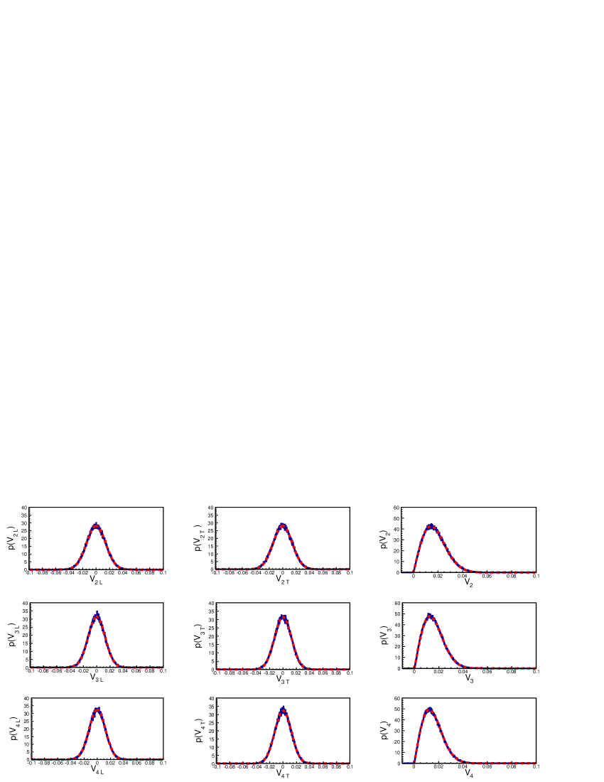
To get some notion for the inherent model fluctuations, we start with HYDJET++ simulations for the simplest case of central PbPb collisions $(b=0)$ in which all azimuthal anisotropy parameters $\epsilon(b)$, $\delta(b)$ and $\epsilon_{3}(b)$ are equal to zero. Figure 1 shows the probability densities both for each component of the flow vector $\vec{V}_{n}$ and for its modulus $V_{n}=|\vec{V}_{n}|$, $n=2,3,4$. In this “fluctuation-only” scenario the probability densities of $\vec{V}_{n}$ are well described by two-dimensional (2D) Gaussian functions Voloshin:2007pc ; Bhalerao:2006tp :

$$p(\vec{V}_{n})=\frac{1}{2\pi\sigma^{2}_{n}}\exp[-\vec{V}_{n}^{2}/(2\sigma^{2}_{n})]~{},$$ (6)

whereas the probability densities of $V_{n}$ have the forms of one-dimensional (1D) Gaussians

$$p(V_{n})=\frac{V_{n}}{\sigma^{2}_{n}}\exp[-V_{n}^{2}/(2\sigma^{2}_{n})]~{},$$ (7)

which are obtained from Eq.(LABEL:eq:4) by integration over the azimuthal angle.

These distributions are characterized by a single parameter $\sigma_{n}$ only, which regulates both the modulus mean $\langle V_{n}\rangle$ and the width $\sigma_{V_{n}}=\sqrt{\langle V_{n}^{2}\rangle-\langle V_{n}\rangle^{2}}$ as

$$\langle V_{n}\rangle=\sqrt{\frac{\pi}{2}}~{}\sigma_{n}~{},$$ (8)

$$\sigma_{V_{n}}=\sqrt{2-\frac{\pi}{2}}~{}\sigma_{n}~{},$$ (9)

$$\frac{\sigma_{V_{n}}}{\langle V_{n}\rangle}=\sqrt{\frac{4}{\pi}-1}~{}=~{}0.523~{}.$$ (10)

In HYDJET++ the value of this fitting parameter, Gaussian width $\sigma_{n}$, appears to be unique for all harmonics with a good enough accuracy: $\sigma_{2}\simeq\sigma_{3}\simeq\sigma_{4}\approx 0.013$. It depends on a number of model parameters, which were already fixed. The main regulator of $\sigma_{n}$ is the mean multiplicity, which determines the variation of $\sigma_{n}(b)$ with centrality.

Recall, that in all Bjorken-like models with cylindrical parameterization the azimuthal anisotropy of the freeze-out surface transforms into the azimuthal anisotropy of particle momentum distribution proportionally to a term $(p_{T}\sinh{Y_{T}}/T)\cos{(\phi-\varphi)}$ Lokhtin:2008xi , arising in scalar product of 4-vectors of particle momentum and flow velocity of the fluid element. Here $\phi$ is the azimuthal angle of the fluid element, $\varphi$ is the particle azimuth, $T$ is the freeze-out temperature and $Y_{T}$ is the transverse flow rapidity, respectively. The pre-factor before the cosine controls the azimuthal angle structure of particle spectrum and its inverse characterizes the fluctuation width squared. We have also verified numerically that at fixed mean multiplicity in selected $p_{T}$ window the width of $\sigma_{n}(p_{T})$ is approximately proportional to the factor $\sqrt{T/(p_{T}\sinh{Y_{T}^{\rm max})}}$, where $Y_{T}^{\rm max}$ is the maximal transverse flow rapidity.

The “true” direction of the flow vector $\vec{V}_{n}$ in HYDJET++ for any azimuthal harmonic is pre-defined in each event. Therefore, $V_{\rm nL}$ can be calculated as a longitudinal component of the actual flow vector along this known direction, and $V_{\rm nT}$ — as a transverse component of $\vec{V}_{n}$ perpendicular to the longitudinal one. As shown in Fig. 1, the mean values of the flow components are zero, $\langle V_{\rm nL}\rangle=\langle V_{\rm nT}\rangle=0,\ n=2,3,4$, and, therefore, $v_{2}=v_{3}=v_{4}$ as it should be in a trivial case of the flow absence in a perfectly central collision.

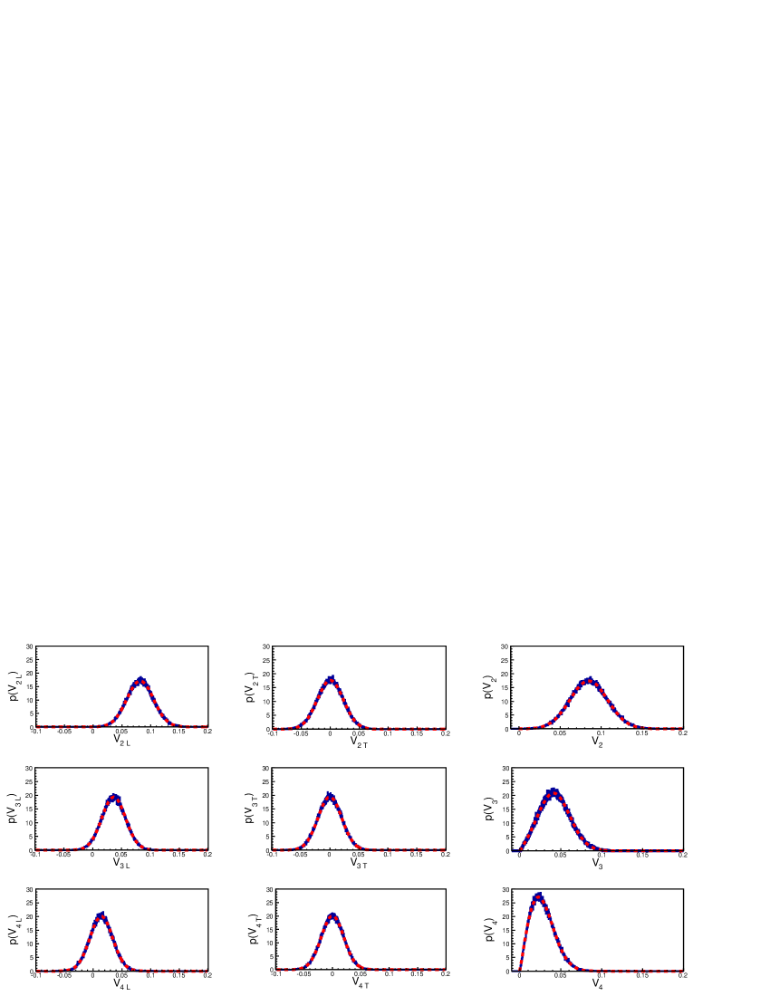
Figure 2 demonstrates the probability densities both for each component of the flow vector $\vec{V}_{n}$ and for its modulus $V_{n}=|\vec{V}_{n}|,\ n=2,3,4$ in the case of non-zero flow vector $\langle V_{\rm nL}\rangle$ in PbPb collisions at centralities $20-25\%$. Instead of distributions (LABEL:eq:4) and (LABEL:eq:5) we get here Voloshin:2007pc ; Bhalerao:2006tp

$$\displaystyle p(V_{\rm nL}) = \frac{1}{\sqrt{2\pi\sigma^{2}_{n}(b)}}\exp\left[-\frac{(V_{\rm nL}-\langle V_{\rm nL}\rangle)^{2}}{2\sigma^{2}_{n}(b)}\right]\ ,$$ (11)

$$p(V_{\rm nT}) = \frac{1}{\sqrt{2\pi\sigma^{2}_{n}(b)}}\exp\left[-\frac{(V_{\rm nT})^{2}}{2\sigma^{2}_{n}(b)}\right]\ ,$$ (12)

$$p(V_{n}) = \frac{V_{n}}{\sigma^{2}_{n}(b)}\exp\left[-\frac{V_{n}^{2}+\langle V_{\rm nL}\rangle^{2}}{2\sigma^{2}_{n}(b)}\right]I_{0}\left(\frac{V_{n}\langle V_{\rm nL}\rangle}{\sigma^{2}_{n}(b)}\right)\ ,$$

where $I_{0}$ is the modified Bessel function of the first kind zero order. Both the width $\sigma_{V_{n}}=\sqrt{\langle V_{n}^{2}\rangle-\langle V_{n}\rangle^{2}}$ and the modulus mean $\langle V_{n}\rangle$ are controlled by the true value of the flow vector $\langle V_{\rm nL}\rangle$ and the width $\sigma_{n}(b)$, but cannot be cast analytically as functions of $\langle V_{\rm nL}\rangle$ and $\sigma_{n}(b)$. Note also that $\langle V_{n}\rangle$ is not equal to $\langle V_{\rm nL}\rangle$ exactly, and the azimuthal anisotropy parameters $\epsilon(b)$, $\delta(b)$ and $\epsilon_{3}(b)$ have been tuned earlier at a given impact parameter $b$ in such a way that the value of $\langle V_{\rm nL}\rangle$ extracted from the distribution (11) reproduces just the experimentally observed value of $v_{\rm n}(b)$ entering in Eq.(1). Similar to the non-flow case, presented in Fig. 1, the widths $\sigma_{n}$ of the longitudinal and transverse distributions shown in Fig. 2 are approximately the same, $\sigma_{2}\simeq\sigma_{3}\simeq\sigma_{4}\approx 0.02$, but the distributions become broader. Also, the maxima of $p(V_{\rm nL})$ and $p(V_{n})$ distributions are shifted towards zero with rising harmonic number $n$, indicating that $v_{2}>v_{3}>v_{4}$ at this centrality. Surely, it is interesting to compare our inherent model probability densities, obtained without any additional special parameters for the azimuthal fluctuations, with the experimental data.

We have also considered including of additional “eccentricity” fluctuations in HYDJET++ model. The simplest modification for this purpose is to introduce event-by-event Gaussian smearing of the spatial anisotropy parameters $\epsilon(b)$ and $\epsilon_{3}(b)$ with the widths proportional to its “unsmeared” values. The coefficients of this proportionality are independent on event centrality and tuned to fit the data. Both model versions, with and without the smearing, are employed for the extraction of the flow fluctuations and comparison with the available experimental data.

3 Unfolding procedure for flow fluctuations analysis

Unfortunately, the direct comparison of the model distributions given by Eqs. (11-2) with the corresponding experimental data is impossible. The EbyE distributions of anisotropic flow harmonics have been obtained by the ATLAS Collaboration Aad:2013xma for the distribution of the modulus of the flow vector by application of the so-called “unfolding procedure”. The goal of the unfolding procedure was to extract the “true” flow vector from the observed one by excluding the influence of non-flow effects, such as resonance decays and jet fragmentation, as well as the finite event multiplicity effect. Therefore, in what follows we will show our results before and after the unfolding to be adequate. In order to employ the EbyE unfolding procedure for simulated events, the analysis method from Aad:2013xma was utilized.

• The EbyE distributions of charged particles in PbPb collisions at $\sqrt{s}_{\rm NN}=2.76$ TeV with $p_{T}>0.5$ GeV/$c$ and $|\eta|<2.5$ are used as input distributions. Fourier decomposition of the azimuthal distribution is rewritten as

  $$\displaystyle\frac{dN}{d\varphi} \propto 1+2\sum^{\infty}_{n=1}V^{\rm obs}_{\rm n}\cos{\left[n(\varphi-\Psi^{\rm obs}_{\rm n})\right]}=$$ (14)

  $$= 1+2\sum^{\infty}_{n=1}(V^{\rm obs}_{\rm n,x}\cos{n\varphi}+V^{\rm obs}_{\rm n,y}\sin{n\varphi})\ ,$$

  where $V^{\rm obs}_{\rm n}$ is the magnitude of the observed per-particle flow vector and $\Psi^{\rm obs}_{\rm n}$ is the event plane angle.

• The single-particle EbyE distributions are constructed and used in our unfolding procedure:

  $$V^{\rm obs}_{\rm n}=\sqrt{(V^{\rm obs}_{\rm n,x})^{2}+(V^{\rm obs}_{\rm n,y})^{2}}\ ,$$

  $$V^{\rm obs}_{\rm n,x}=V^{\rm obs}_{\rm n}\cos{n\Psi^{\rm obs}_{\rm n}}=\langle\cos{n\varphi}\rangle\ ,$$ (15)

  $$V^{\rm obs}_{\rm n,y}=V^{\rm obs}_{\rm n}\sin{n\Psi^{\rm obs}_{\rm n}}=\langle\sin{n\varphi}\rangle\ .$$

  The averaging in last two equations of (LABEL:eq:13) is performed over all hadrons in a single event. As was shown in Aad:2013xma , the distribution obtained after the unfolding procedure did not depend on the method applied to obtain $V^{\rm obs}_{\rm n}$. Thus, the single-particle method can be used for our study.

• The response function is constructed using the “two sub-event method” (2SE), namely, the charged particles are divided into two sub-events with $\eta<0$ and $\eta>0$. The smearing effects are estimated by the difference of the flow vectors between the two sub-events, for which the flow signal cancels. This distribution is fitted to the Gaussian with the width $\delta_{\rm 2SE}$ determined mainly by the finite multiplicity effect and the non-flow contributions. It was shown in Aad:2013xma that the response function constructed by such a procedure can be expressed as

  $$p(V^{\rm obs}_{\rm n}|V_{\rm n})\propto V^{\rm obs}_{\rm n}\exp\left[-\frac{(V^{\rm obs}_{\rm n})^{2}+V^{2}_{\rm n}}{2\delta^{2}}\right]I_{0}\left(\frac{V^{\rm obs}_{\rm n}V_{\rm n}}{\delta^{2}}\right)\ .$$

  Here $\delta=\delta_{\rm 2SE}/2$ because we use the full-event $V^{\rm obs}_{\rm n}$ distribution as an input, and $\delta_{\rm 2SE}$ is the width obtained from the difference between the EbyE per-particle flow vectors of the two sub-events.

• The constructed response function is used to obtain the unfolding matrix:

  $$M_{ij}^{\rm iter}=\frac{A_{ji}c_{i}^{\rm iter}}{\Sigma_{m,k}A_{mi}A_{jk}c_{k}^{\rm iter}},$$

  $$\widehat{c}^{\rm iter+1}=\widehat{M}^{\rm iter}\widehat{e},A_{ji}=p(e_{j}|c_{i})~{},$$ (17)

  where $A_{ji}$ is the response function between $e_{j}=V^{\rm obs}_{\rm n}$ (“effect”) and $c_{i}=V_{\rm n}$ (“cause”). The true $V_{\rm n}$ distribution (cause “c”) is obtained from the measured $V^{\rm obs}_{\rm n}$ distribution (effect “$e$”) using an iterative algorithm. Then the Bayesian unfolding procedure is performed by means of the RooUnfold package Adye .

The difference between the $\delta_{\rm 2SE}$ and $\sigma_{n}$ arises mostly due to the dynamical flow fluctuations. Therefore, the EbyE unfolding analysis excludes the effects related to $\delta_{\rm 2SE}$, and leaves the genuine flow fluctuations.

The application of Bayesian unfolding method for the anisotropic flow analysis was checked with heavy ion event generators in JiaMoham . It was shown that the restored density distributions were able to reproduce the input $V_{n}$ distributions. The non-flow effects were estimated by using the HIJING event generator hijing with and without the implementation of the flow signal, and were found to be of the order of statistical errors. In case of the AMPT model ampt , which includes both flow and non-flow fluctuations, the difference between the “generated” and “unfolded” flow harmonics in semiperipheral Au+Au collisions at RHIC was found to be small for elliptic flow and significantly increasing in the tails for triangular and quadrangular flows. Fluctuations originated from the finite multiplicity effect can be evaluated under the assumption of Gaussian multiplicity distribution JiaMoham :

$$\delta_{n}=\sqrt{\Big{\langle}\frac{1}{2N}\Big{\rangle}}\simeq\sqrt{\frac{1}{2\langle N\rangle}\Big{[}1+\Big{(}\frac{\sigma_{N}}{\langle N\rangle}\Big{)}^{2}\Big{]}}~{},$$ (18)

where $\langle N\rangle$ and $\sigma_{N}$ are the mean value and the width of the distribution, respectively.

4 Comparison of HYDJET++ simulations with LHC data

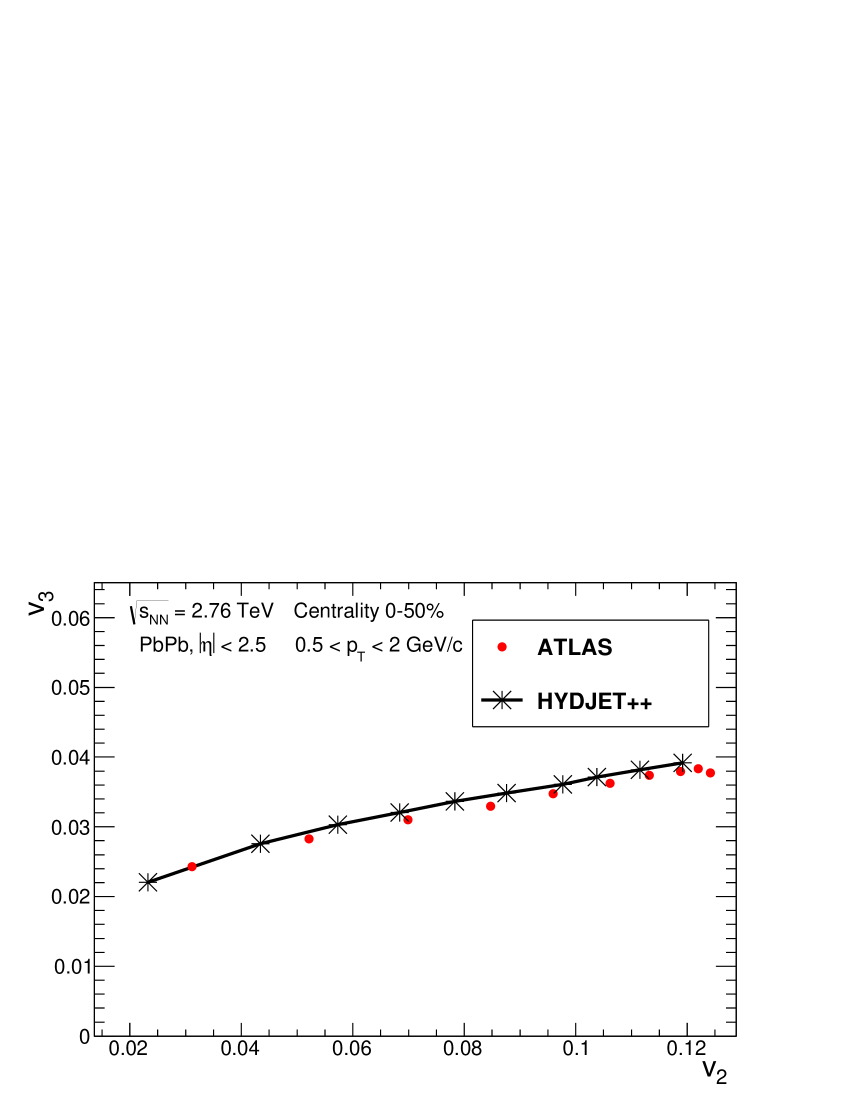
At first we have checked that HYDJET++ reproduces well the experimentally measured correlation between the event-averaged elliptic and triangular flow coefficients. The results of model simulations are plotted onto the ATLAS data Aad:2015lwa in Fig. 3. One can see that the calculations and the data agree well within the 7% accuracy limit.

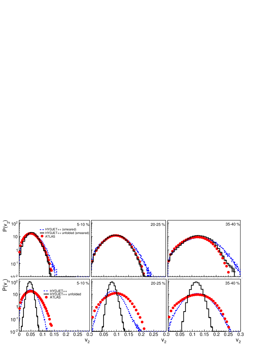
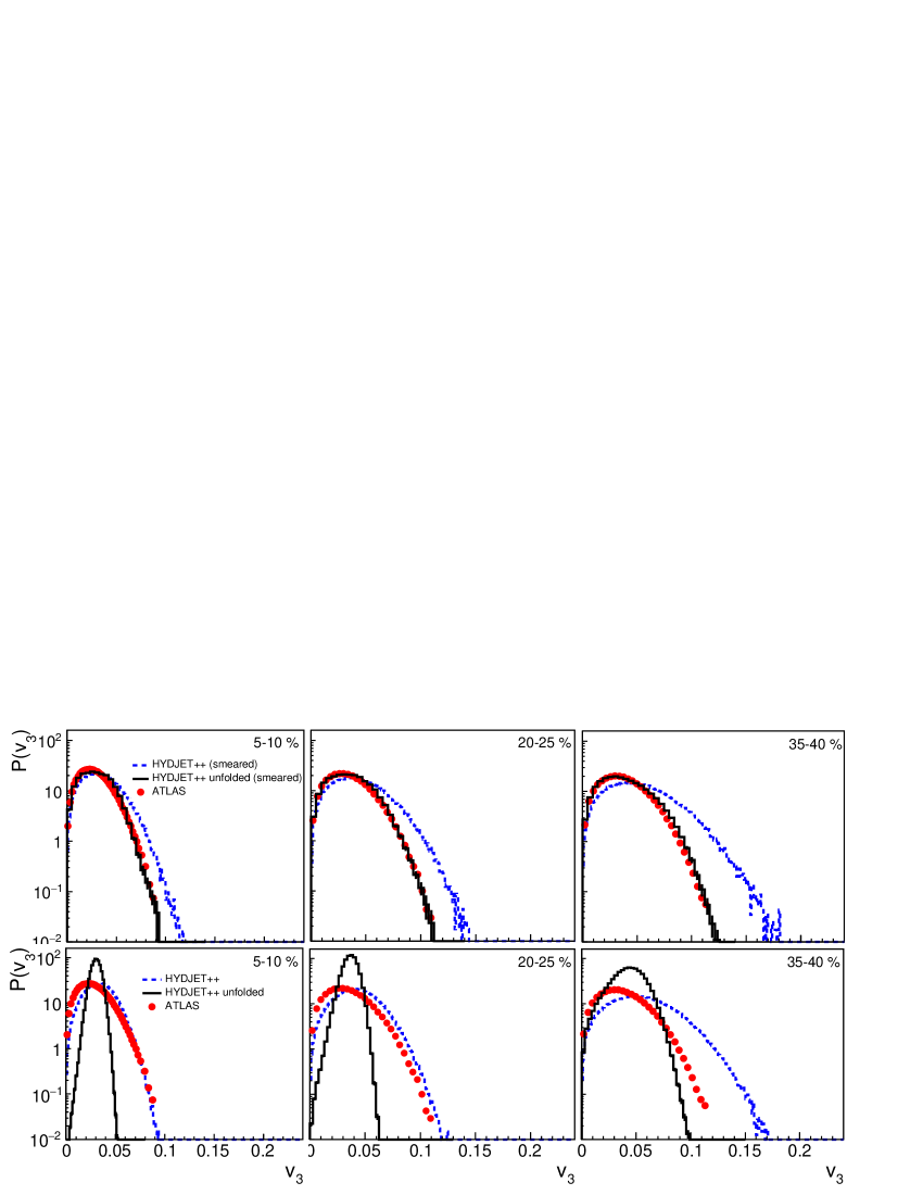
Then, we consider the anisotropic flow fluctuations. The simulations and analysis were performed for three centrality intervals, namely, $5-10\%$, $20-25\%$ and $35-40\%$, and for two settings of the HYDJET++ model: (i) without and (ii) with the additional smearing of spatial anisotropy parameters $\epsilon(b)$ and $\epsilon_{3}(b)$, see Sec. 2. The results for $p(V_{2})$ and $p(V_{3})$ are presented in Fig. 4 and Fig. 5, respectively, and listed in Table 1. Both figures indicate that the original version of HYDJET++ (without the smearing of $\epsilon(b)$ and $\epsilon_{3}(b)$) already includes some dynamical fluctuations due to radial flow. Moreover, the mean values of $\langle V_{n}\rangle$ and widths of the distributions $\sigma_{V_{n}}$ in the default version of HYDJET++ are quite close to the measured ones in collisions with centralities up to 25% for the triangular flow and up to 45% for the elliptic flow, see Table 1. Although the agreement can be further improved by rescaling of $\langle V_{n}\rangle$ to match the data, such approach would be completely misleading. Implementation of the unfolding procedure clearly demonstrates in Figs. 4,5 that the initial distributions become more narrow. Thus, the intrinsic fluctuations appear to be too weak to match the experimental data Aad:2013xma . On the other hand, simple modification of the model via introducing the normal distribution over the spatial anisotropy parameters allows us to reproduce the measured event-by-event fluctuations of elliptic and triangular flow, the distribution widths and the event-averaged values of $\langle V_{2}\rangle$ and $\langle V_{3}\rangle$. The distributions $p(V_{n})$ obtained with the set of the smeared out parameters are broader in the tails compared with the experiment. Unfolding makes it narrower. Here the difference between the “initial” and “unfolded” spectra are not so dramatic although still noticeable in contrast to that at RHIC energy, calculated in JiaMoham within the AMPT model. The two additional parameters of the model, appeared in this case, are the coefficients of proportionality between the Gaussian widths of the distributions $p(\epsilon)$ and $p(\epsilon_{3})$ and their “unsmeared” values. These two coefficients are fixed to fit the data on $p(V_{2})$ and $p(V_{3})$, respectively, for only one arbitrary centrality, whereas for other centralities they are the same.

It is worth noting, that such a simple modification of the model also increases EbyE fluctuations for higher order harmonics $v_{n}$ ($n>3$), which arise in HYDJET++ due to the presence of elliptic $v_{2}$ and triangular $v_{3}$ flows, and its interference. However, significant sensitivity of high harmonic values on their extraction methods makes the direct comparison of our simulations with the data even more tricky than for $v_{2}$ and $v_{3}$. For example, the centrality dependence of quadrangular flow $v_{4}$ measured by event plane and two-particle cumulant methods is significantly weaker than that of $v_{4}$ measured by Lee-Yang zero method due to large non-flow contribution and increase of the flow fluctuations in more central events. Since HYDJET++ was tuned to fit the $p_{\rm T}$ -dependence of $v_{4}\{LYZ\}$, it underestimates $v_{4}$ extracted by the event plane or two-particle cumulant methods in (semi)central collisions Bravina:2013xla . We plan to study the event-by-event fluctuations of higher order flow harmonics in the future.

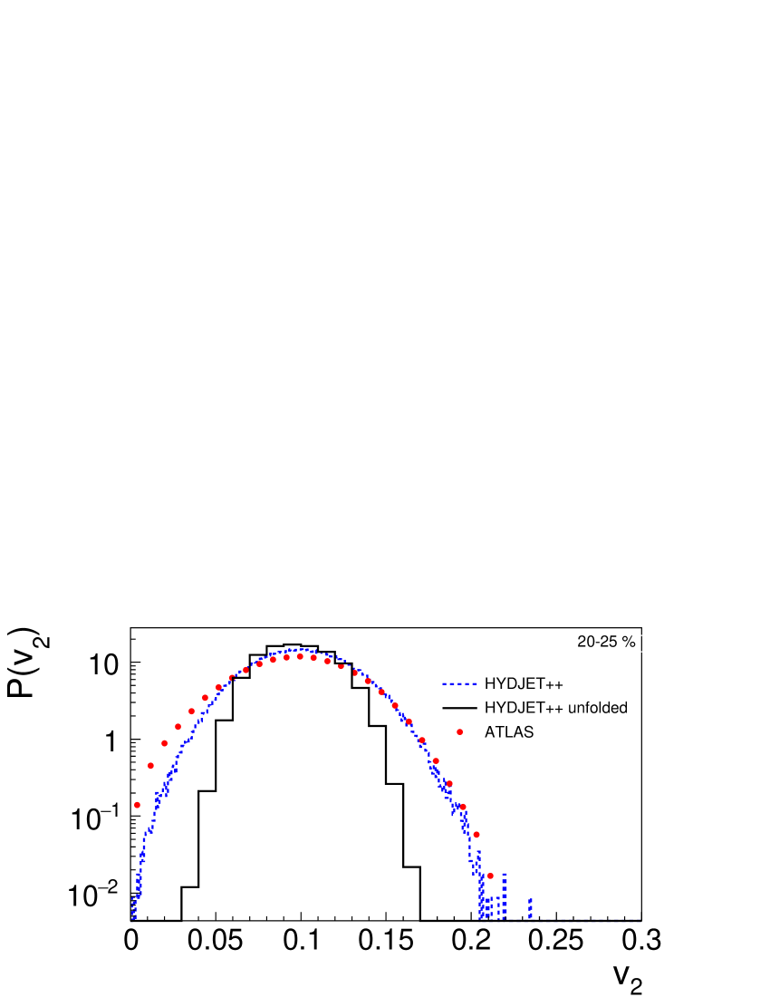
Few important issues should be clarified still. We utilized normal smearing of the parameters $\epsilon(b),\delta(b)$ and $\epsilon_{3}(b)$ in the modified version of the event generator. What will happen if the parameters are smeared out with respect to a non-Gaussian distribution? To check this possibility we opted for a uniform distribution of the key parameters within the interval $\pm\sigma_{\epsilon}$ to ensure the same mean and width values. The distribution $p(V_{2})$ is displayed in Fig. 6 for centrality bin $20-25\%$, where the signal heavily dominates over the fluctuations. Interestingly enough, the generated distribution is very close to the ATLAS unfolded curve everywhere, but in the low-$V_{2}$ range. Unfolded HYDJET++ spectrum, however, is narrow. It resembles the implemented rectangular-shaped $V_{2}$-distribution with some rounding of the shoulders because of the intrinsic model fluctuations.

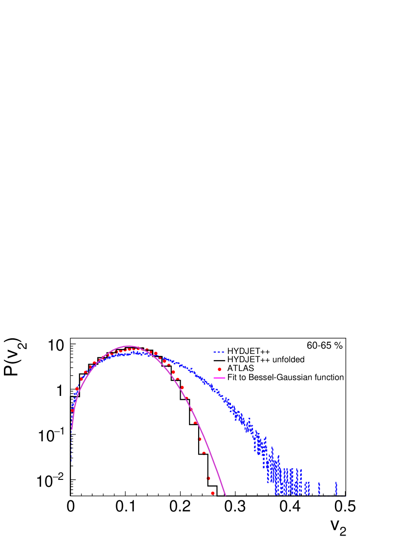
Next question is the Gaussian-like behavior of the obtained spectra after the unfolding. ATLAS Collaboration reported some deviations from the Gaussians observed for $p(V_{2})$ distributions in peripheral collisions Aad:2015lwa . The last centrality bin in ATLAS analysis is $60-65\%$. At this centrality the default version of HYDJET++, which works reasonably well up to $40-45\%$ Lokhtin:2008xi , needs further fine tuning in line with other semi-phenomenological models. Simply, the linear dependence for $v_{2}(b)$ becomes too crude here. The new tuned values of the parameters are $\epsilon=0.14$ and $\delta=0.25$ (cf. with $\epsilon=0.16$ and $\delta=0.38$ in the default version). It is worth noting that this is the only modification of the model, whereas the ratio $\langle\epsilon\rangle/\sigma_{\epsilon}$ is kept constant for all centralities in question. Figure 7 shows the observed and the unfolded distributions of $p(V_{2})$ obtained in HYDJET++ for centrality $60-65\%$ in comparison with the ATLAS data. One can see that the model calculations agree well with the data. The unfolded distribution provided by HYDJET++ was also fitted to complex Bessel-Gauss (BG) product given by Eq. (2). Results are plotted onto the simulated spectra in Fig. 7 as well. At this centrality the BG fit clearly deviates from the data indicating that the model possesses some intrinsic fluctuations which cause the distortion of initial Gaussians. This interesting problem definitely deserves further investigations.

Finally, our results can be used for the analysis of fluctuations of the initial anisotropy $\varepsilon_{n}$. This approach relies on the assumption of a linear response of the flow coefficient $V_{n}$ to the corresponding initial eccentricity

$$V_{n}=k_{n}~{}\varepsilon_{n}\ ,$$ (19)

where $k_{n}$ is the response coefficient. For both elliptic and triangular flow this assumption works very well, as was confirmed by hydrodynamic model calculations Qiu:2011iv ; Niemi:2012aj . The probability distribution of the flow is connected to the initial anisotropy distribution via Yan:2014nsa

$$p(V_{n})=\frac{d\varepsilon_{n}}{dV_{n}}~{}p(\varepsilon_{n})~{}.$$ (20)

Inserting Eq. (LABEL:eq:17) into Eq. (LABEL:eq:18) we get

$$p(\varepsilon_{n})=k_{n}~{}p(V_{n})~{}.$$ (21)

Then, in Yan:2014afa the Elliptic Power distribution was proposed to parametrize the eccentricity distributions

$$p(\varepsilon_{n})=\frac{2\alpha\varepsilon_{n}}{\pi}(1-\varepsilon_{0}^{2})^{\alpha+1/2}\int_{0}^{\pi}\frac{(1-\varepsilon_{n}^{2})^{\alpha-1}d\varphi}{(1-\varepsilon_{0}\varepsilon_{n}\cos{\varphi)}^{2\alpha+1}}~{}.$$

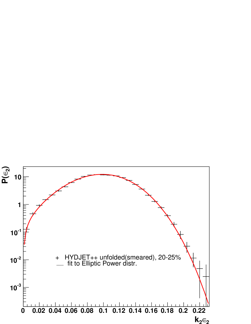
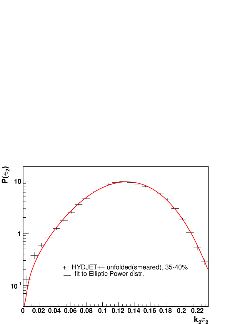
Here the parameter $\varepsilon_{0}$ is approximately the mean reaction plane eccentricity and $\alpha$ describes the eccentricity fluctuations. In Yan:2014nsa the authors fitted the ATLAS data on the elliptic flow to Eq. (LABEL:eq:20). It is very tempting, therefore, to fit the HYDJET++ generated distributions to Eq. (LABEL:eq:20) and compare the extracted parameters, $\alpha,\ \varepsilon_{0}$ and $k_{2}$. The fitted curves are plotted onto the model calculations (with smearing and unfolding procedure) of $p(\varepsilon_{2})$ distributions for two centralities, $20-25\%$ and $35-40\%$, in Fig. 8. Extracted fit parameters are compared in Table 2 with those obtained in Yan:2014nsa . The agreement between the two sets is good, indicating that HYDJET++ quantitatively reproduces the anisotropic flow fluctuations.

5 Conclusions

The phenomenological analysis of the event-by-event distributions of anisotropic flow harmonics measured in lead-lead collisions at the center-of-mass energy 2.76 TeV per nucleon pair has been performed within the two-component HYDJET++ model. The unfolding procedure was applied to examine the simulated events, thus allowing for the direct comparison of model calculations with the experimental data. To our best knowledge, this is for the first time when the model-generated spectra are filtered by means of the unfolding procedure and then compared directly with the LHC data obtained by the same method. This procedure removes the non-flow effects, originating, e.g., from the decays of resonances and fragmentation of jets, as well as the finite event multiplicity effect.

The essentially dynamical origin of the flow fluctuations in hydro-inspired freeze-out approach has been established. The effect is traced to the correlation between the momenta and coordinates of final particles and the velocities of hadronic fluid elements. The simple modification of the model via introducing the distribution over spatial anisotropy parameters permits HYDJET++ to reproduce both elliptic and triangular flow fluctuations in heavy ion collisions at the LHC energy. In contrast, an attempt to utilize the uniform non-Gaussian smearing with the same $\langle\epsilon\rangle/\sigma_{\epsilon}$ ratio failed shortly. The unfolding procedure is sensitive, therefore, to the initial distributions of the parameters. It should be implemented in any model in case of comparison with the unfolded data.

For the peripheral topologies the model calculations deviate from the Bessel-Gaussian fit to Eq.(2) thus hinting for some intrinsic fluctuations in HYDJET++ which cause the distortion of initial Gaussians. This interesting problem deserves to be studied in the future.

Figure 1: The probability density distributions for two components of the flow vector, $V_{\rm nT}$ and $V_{\rm nL}$, and for its modulus $V_{n}=|\vec{V}_{n}|,\ n=2,3,4$ in the case of zero signal in HYDJET++ (central PbPb collisions at impact parameter $b=0$). Dashed curves on the left and middle plots show two-dimensional fit of simulated HYDJET++ points to Eq. (LABEL:eq:4); dashed curves on the right plots present the 1D-fit to Eq. (LABEL:eq:5).

Figure 2: The same as Fig. 1 but for non-zero signal in HYDJET++ (20-25 % centrality of PbPb collisions). Dashed curves in the left, middle and right columns indicate the fit of simulated HYDJET++ points to Eqs. (11), (12) and (2), respectively.

Figure 3: The correlation between the event-averaged elliptic flow $v_{2}$ and triangular flow $v_{3}$ of charged hadrons at transverse momentum $0.5<p_{\rm T}<2$ GeV/$c$ and pseudo-rapidity $|\eta|<2.5$ for ten 5%-centrality intervals in the centrality range $0-50\%$ of PbPb collisions at $\sqrt{s}_{\rm NN}=2.76$ TeV. Closed circles denote ATLAS data from Aad:2015lwa , asterisks represent HYDJET++ events. Line is drawn to guide the eye.

Figure 4: The probability density distributions of elliptic flow $V_{2}$ in three centrality intervals $5-10\%$ (left), $20-25\%$ (middle) and $35-40\%$ (right). Dashed and solid histograms present the results for simulated HYDJET++ events before and after the unfolding procedure, respectively. The top/bottom row shows the model results with/without the additional smearing of spatial anisotropy parameters. The closed points are ATLAS data from Aad:2013xma .

Figure 5: The same as Fig. 4 but for the triangular flow $V_{3}$ in three centrality intervals.

Figure 6: The probability density distributions of elliptic flow $V_{2}$ in centrality interval $20-25\%$ obtained with uniformly smeared parameters $\epsilon$ and $\delta$. Dashed and solid histograms present the results for simulated HYDJET++ events before and after the unfolding procedure, respectively. ATLAS data are shown by full circles.

Figure 7: The same as upper row of Fig. 4 but for the centrality interval $60-65\%$ only. Dashed and solid histograms present the results for simulated HYDJET++ events before and after the unfolding procedure, respectively. ATLAS data are shown by full circles. Solid curve shows the Bessel-Gauss fit to Eq.(2).

Figure 8: The probability densities $P(\varepsilon_{n})$ obtained in HYDJET++ calculations (with smearing and unfolding) of PbPb collisions at $\sqrt{s_{\rm NN}}=2.76$ TeV with centrality $20-25\%$ and $35-40\%$. Full lines represent the fits to the Elliptic Power distribution (LABEL:eq:20).

	Centrality	$5-10\%$	$20-25\%$	$35-40\%$
	$\langle V_{2}\rangle$	0.0522	0.0976	0.1186
ATLAS	$\sigma_{V_{2}}$	0.0226	0.0330	0.0422
	$\sigma_{V_{2}}/\langle V_{2}\rangle$	0.433	0.338	0.356
	$\langle V_{2}\rangle$	0.0489	0.0853	0.1213
HYDJET++	$\sigma_{V_{2}}$	0.0170	0.0231	0.0353
	$\sigma_{V_{2}}/\langle V_{2}\rangle$	0.347	0.271	0.291
	$\langle V_{2}\rangle$	0.0460	0.0823	0.1163
HYDJET++	$\sigma_{V_{2}}$	0.0081	0.0095	0.0147
unfolded	$\sigma_{V_{2}}/\langle V_{2}\rangle$	0.176	0.116	0.126
	$\langle V_{2}\rangle$	0.0580	0.0999	0.1309
HYDJET++	$\sigma_{V_{2}}$	0.0240	0.0371	0.0483
(smeared)	$\sigma_{V_{2}}/\langle V_{2}\rangle$	0.414	0.371	0.369
HYDJET++	$\langle V_{2}\rangle$	0.0552	0.0971	0.1267
unfolded	$\sigma_{V_{2}}$	0.0199	0.0320	0.0408
(smeared)	$\sigma_{V_{2}}/\langle V_{2}\rangle$	0.361	0.330	0.322
	Centrality	$5-10\%$	$20-25\%$	$35-40\%$
	$\langle V_{3}\rangle$	0.0281	0.0344	0.0373
ATLAS	$\sigma_{V_{3}}$	0.0147	0.0178	0.0192
	$\sigma_{V_{3}}/\langle V_{3}\rangle$	0.522	0.518	0.513
	$\langle V_{3}\rangle$	0.0341	0.0428	0.0555
HYDJET++	$\sigma_{V_{3}}$	0.0139	0.0185	0.0268
	$\sigma_{V_{3}}/\langle V_{3}\rangle$	0.408	0.432	0.482
	$\langle V_{3}\rangle$	0.0304	0.0363	0.0425
HYDJET++	$\sigma_{V_{3}}$	0.0059	0.0067	0.0142
unfolded	$\sigma_{V_{3}}/\langle V_{3}\rangle$	0.195	0.184	0.334
	$\langle V_{3}\rangle$	0.0350	0.0438	0.0527
HYDJET++	$\sigma_{V_{3}}$	0.0178	0.0225	0.0276
(smeared)	$\sigma_{V_{3}}/\langle V_{3}\rangle$	0.509	0.514	0.524
HYDJET++	$\langle V_{3}\rangle$	0.0297	0.0356	0.0387
unfolded	$\sigma_{V_{3}}$	0.0148	0.0180	0.0203
(smeared)	$\sigma_{V_{3}}/\langle V_{3}\rangle$	0.499	0.504	0.526

Table 1: Mean values $\langle V_{n}\rangle$, widths $\sigma_{V_{n}}$ and ratios $\sigma_{V_{n}}/\langle V_{n}\rangle$ (n=2,3) for HYDJET++ simulations and ATLAS data Aad:2013xma .

	Centrality	$20-25\%$	$35-40\%$
	$\alpha$	$56\pm 6$	$24\pm 3$
ATLAS	$\varepsilon_{0}$	$0.25\pm 0.02$	$0.31\pm 0.08$
(reanalysis in Yan:2014nsa )	$k_{2}$	$0.40\pm 0.02$	$0.35\pm 0.01$
	$\alpha$	$48\pm 7$	$35\pm 3$
HYDJET++	$\varepsilon_{0}$	$0.25\pm 0.02$	$0.30\pm 0.01$
(smeared and unfolded)	$k_{2}$	$0.40\pm 0.02$	$0.36\pm 0.02$

Table 2: Parameters of the fit of eccentricity distributions to Eq. (LABEL:eq:20). See text for details.