Estimating the power spectrum covariance matrix with fewer mock samples

Abstract

The covariance matrices of power-spectrum ($P(k)$) measurements from galaxy surveys are difficult to compute theoretically. The current best practice is to estimate covariance matrices by computing a sample covariance of a large number of mock catalogues. The next generation of galaxy surveys will require thousands of large volume mocks to determine the covariance matrices to desired accuracy. The errors in the inverse covariance matrix are larger and scale with the number of $P(k)$ bins, making the problem even more acute. We develop a method of estimating covariance matrices using a theoretically justified, few-parameter model, calibrated with mock catalogues. Using a set of 600 BOSS DR11 mock catalogues, we show that a seven parameter model is sufficient to fit the covariance matrix of BOSS DR11 $P(k)$ measurements. The covariance computed with this method is better than the sample covariance at any number of mocks and only $\sim$100 mocks are required for it to fully converge and the inverse covariance matrix converges at the same rate. This method should work equally well for the next generation of galaxy surveys, although a demand for higher accuracy may require adding extra parameters to the fitting function.

1 Introduction

The covariance matrix and inverse covariance matrix of the band averaged power spectrum are crucial for parameter estimation from cosmological spectroscopic surveys. Having an accurate estimate of the covariance matrix, and therefore the inverse covariance matrix, is paramount in order to be able to assign reliable uncertainties in estimated parameters (Percival et al., 2014). Most studies achieve this by using a large number of mock samples (Cole et al., 2005; Reid et al., 2010; Manera et al., 2013, 2015; Anderson et al., 2014; Gil-Marín et al., 2015) setup to match the characteristics of the particular survey, and then running them through the data pipeline to estimate the covariance matrix via

$$C_{ij}=\dfrac{1}{N-1}\sum_{s}\left(P_{i}^{s}-\mu_{i}\right)\left(P_{j}^{s}-\mu_{j}\right),$$ (1)

where $N$ is the number of mocks,

$$\mu_{i}=\dfrac{1}{N}\sum_{s}P_{i}^{s},$$ (2)

and $P_{i}\equiv P(k_{i})$.

The elements of the sample covariance matrix converge as $\mathcal{O}\left(N^{-1}\right)$ to their true values, while the inverse covariance matrix elements converge as $\mathcal{O}\left(N_{\mathrm{b}}/N\right)$, where $N_{\mathrm{b}}$ is the number of $P(k)$ bins (see e.g., Anderson, 2003). This inaccuracy propagates into derived cosmological parameters and inflates their errorbars by a factor of $\mathcal{O}\left(1+N_{\mathrm{b}}/N\right)$ (Hartlap et al., 2007; Taylor et al., 2013; Percival et al., 2014; Dodelson & Schneider, 2013; Taylor & Joachimi, 2014). Percival et al. (2014) found that in order for this extra variance to be sub-dominant for Baryon Oscillation Spectroscopic Survey (BOSS; Eisenstein et al., 2011; Dawson et al., 2013) Data Release (DR) 9 measurements $\sim 600$ mock catalogues were needed. The next generation of galaxy surveys will have more stringent requirements on the precision of the covariance matrix and will require even larger sets of mock catalogues to compute the sample variance. Taylor et al. (2013) estimated that up to $10^{6}$ mocks may be required for the joint analysis of future galaxy clustering and weak lensing data.

There are a number of methods with which one can generate these mock catalogues that tend to reduce the computational cost, such as the log-normal method (Coles & Jones, 1991), pinpointing orbit-crossing collapsed heirarchical objects (pinocchio; Monaco et al., 2002; Monaco et al., 2013), comoving lagrangian acceleration simulations (cola; Tassev et al., 2013), perturbation theory catalogue generator of halo and galaxy distributions method (patchy; Kitaura et al., 2014, 2015), pertabuation theory halos method (pthalos; Scoccimarro & Sheth, 2002; Manera et al., 2013, 2015), or quick particle mesh method (qpm; White et al., 2014). Chuang et al. (2015) provide detailed descriptions and a comparison of the effectiveness of mocks generated using these techniques, concluding that the more efficient approximate solvers can be used to reach a few per cent accuracy for clustering statistics on scales of interest for large-scale structure analyses.

However, with surveys such as the Dark Energy Survey (DES; Frieman & Dark Energy Survey Collaboration, 2013), the upcoming Dark Energy Spectroscopic Instrument survey (DESI; Schlegel et al., 2011; Levi et al., 2013), Extended Baryon Oscillation Spectroscopic Survey (eBOSS; Schlegel et al., 2009), Large Synoptic Survey Telescope surveys (LSST; LSST Science Collaboration et al., 2009), Euclid satellite mission surveys (Laureijs et al., 2011), and numerous others increasing the volumes to be analysed, the mocks must also increase in volume. This can still lead to situations where the computational costs of generating the necessary number of mocks becomes prohibitive, making it desirable to have a method of estimating the true covariance matrix using fewer mock catalogues.

The use of mock catalogues can be completely bypassed by looking at the intrinsic scatter of $P(k)$ measurements within the sample e.g. using the jack-knife or bootstrap methods. The jack-knife method is limited by the fact that to build up better statistics one must divide the survey data into smaller and smaller subvolumes, limiting the maximum scale for which the covariance can be reliably measured (Norberg et al., 2009; Beutler et al., 2011). The bootstrap method performs better but is still limited by the number of subvolumes that can be created from the data (see Norberg et al., 2009, for a detailed discussion of the two methods).

In principle, the covariance of $P(k)$ measurements can be computed theoretically. Nonlinear effects in structure growth and highly nontrivial survey windows make this kind of computation difficult in practice. Despite this, several recent works demonstrated that this approach can be used to derive reasonably good approximations to the covariance matrix (for recent work see e.g., de Putter et al., 2012, and references therein). Similar efforts have been applied to the correlation function (inverse Fourier transform of $P(k)$) covariance matrices (see e.g., Xu et al., 2012).

Alternative approaches include using a shrinkage estimation (Pope & Szapudi, 2008; de la Torre et al., 2013), covariance tapering (Paz & Sanchez, 2015) and using a small number of mocks while ‘resampling’ large-scale Fourier modes (Schneider et al., 2011).

In this paper we propose a new approach to estimating $P(k)$ covariance matrices. We start with a brief overview of the theory behind $P(k)$ covariance matrices in section 2. Then we describe the mock catalogues along with our procedure for estimating the power spectrum, true covariance and inverse covariance matrix, and their associated uncertainties, from those catalogues in section 3.

In section 4, we choose a theoretically justified functional form with a small number of free parameters to describe the covariance matrix and use mock catalogues to calibrate numerical values of parameters. Unlike previous approaches based on theoretical modelling we put significantly less stress (and effort) into computing the actual covariance matrix elements; ‘Back of the envelope’ theoretical considerations are only used as a rough guide in justifying the functional form and the actual numbers come purely from the fit to the mock sample covariance matrices. In section 5 we show that a simple seven parameter model is good enough to describe the covariance matrix of the BOSS DR11 sample as computed from a sample of 600 mocks. In the range of scales relevant for the baryon acoustic oscillation (BAO) peak and the redshift-space distortion measurements ($0<k<0.2h\ \mathrm{Mpc}$) our fitting function works exceptionally well.

We also show in section 5 that the procedure converges much better than the sample covariance with the number of mocks used. At any number of mocks, the fitted covariance matrix is closer to the final result than the corresponding sample covariance matrix, and at $N\sim 100$ the fitted covariance matrix is already statistically indistinguishable from the sample covariance matrix computed with $N=600$. The inverse covariance matrix converges at the same rate as the covariance matrix. Demand for higher accuracy may require introducing additional free parameters into the fitting function, but there is no reason why this method should not work equally well for the future galaxy surveys. These conclusions are summarized in section 6, where we also discuss planned further work.

2 Theoretical $P(k)$ covariance

For a Gaussian field in a large uniform volume the covariance matrix of $P(k)$ estimated in bins of width $\delta k$ is

$$C_{ij}=\frac{(2\pi)^{3}}{V}\frac{\left(P_{i}+n^{-1}\right)^{2}}{2\pi k_{i}^{2}\delta k}\delta_{ij},$$ (3)

where $V$ is the volume of the survey and $n$ is the number density of galaxies (Feldman et al., 1994; Tegmark, 1997). When the number density of galaxies is not constant across the survey this changes to

$$C_{ij}=\frac{(2\pi)^{3}}{V_{\mathrm{eff}}(k_{i})}\frac{P^{2}_{i}}{2\pi k_{i}^{2}\delta k}\tilde{\delta}_{ij},$$ (4)

with

$$V_{\mathrm{eff}}(k_{i})\equiv\displaystyle\int\displaylimits_{V}\!\mathrm{d}^{3}r\,\frac{\left[P^{2}_{i}n(\bm{r})+1\right]^{2}}{P^{2}_{i}n^{2}(\bm{r})}.$$ (5)

If, in addition, the width of the k-bins is comparable to $1/V$, the finite volume will result in the coupling of neighbouring $P(k)$ measurements and the Kronecker delta function in Eq. (4) will turn into

$$\delta_{ij}\rightarrow\tilde{\delta}_{ij}=\displaystyle\int\displaylimits_{V}\!\mathrm{d}^{3}r\,\mathrm{e}^{-\mathrm{i}(\bm{k}_{i}-\bm{k}_{j})\cdot\bm{r}}.$$ (6)

The observed volume $V$ is usually highly nontrivial which makes the effective volume difficult to compute. Nonlinear effects in structure growth and galaxy biasing further complicate matters, adding terms proportional to the bin averaged trispectrum, $\overline{T}(k_{i},k_{j})$, to the off-diagonal elements of the covariance matrix, resulting in

$$C_{ij}=\frac{(2\pi)^{3}}{V_{\mathrm{eff}}(k_{i})}\left(\frac{P^{2}_{i}}{2\pi k_{i}^{2}\delta k}\delta_{ij}+\overline{T}(k_{i},k_{j})\right)$$ (7)

(see Scoccimarro et al. 1999 and Bernardeau et al. 2002 for details).

3 Measuring $P(k)$ covariance from BOSS DR11 mocks

While it is possible, in principle, to compute the covariance of $P(k)$ measurements from Eq. (7), highly nontrivial survey windows and the introduction of terms dependent on the trispectrum from nonlinear structure growth make this difficult in practice. Therefore, in order to obtain an estimate of the true covariance matrix, we use 600 BOSS DR11 pthalos mock catalogues (Manera et al., 2013) to compute the sample covariance of the spherically averaged $P(k)$. For simplicity we only use the mocks for the North Galactic Cap (NGC). We use the same estimator, weighting scheme, and shot noise subtraction method as the latest official DR11 analyses papers (see e.g., Gil-Marín et al., 2015). We estimate the spherically averaged $P(k)$ in 23 bins of width $\Delta k=0.008h~{}\mathrm{Mpc}^{-1}$ in the wavelength range $0.0\leq k\leq 0.184h~{}\mathrm{Mpc}^{-1}$. We then compute the sample covariance matrix using Eqs. (1) and (2).

Figure 1 shows the average $P(k)$ with the errorbars computed by taking a square root of diagonal elements of the covariance matrix ($\sqrt{C_{ii}}$). Figure 2 shows the elements of the reduced covariance matrix defined as

$$r_{ij}\equiv\dfrac{C_{ij}}{\sqrt{C_{ii}C_{jj}}}.$$ (8)

Figure 1: The average of the power spectra from the 600 CMASS NGC pthalos mocks. The error bars are the square root of the diagonal elements of the sample covariance matrix calculated from all 600 mocks.

Figure 2: The reduced covariance matrix calculated with all 600 NGC pthalos mocks. See the online article for a colour version of this plot.

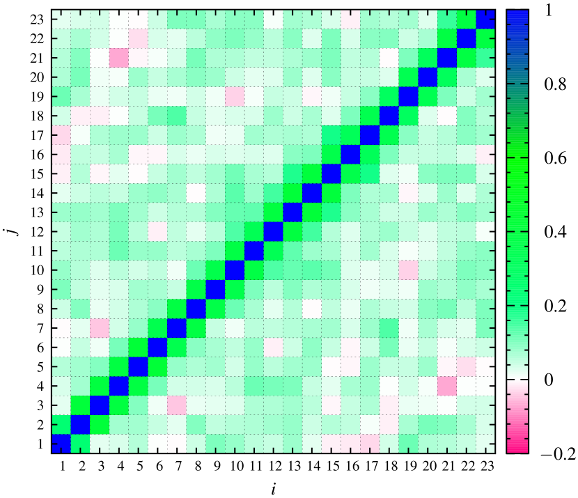
Assuming that the distribution of individual $P(k)$ measurements is close to Gaussian, the measured $C_{ij}$ follow the Wishart distribution (Anderson, 2003). In the limit of large $N$ the Wishart distribution tends to a Gaussian distribution with the covariance matrix

$$\langle C_{ij}C_{kl}\rangle=\frac{\sigma_{i}\sigma_{j}\sigma_{k}\sigma_{l}}{N}(r_{ik}r_{jl}+r_{il}r_{jk}),$$ (9)

where $\sigma_{i}$ and $r_{ij}$ are the unknown true variance and cross-correlation coefficients of power spectrum band estimates. The variance in both diagonal,

$$\langle C_{ii}^{2}\rangle=\frac{2\sigma_{i}^{4}}{N},$$ (10)

and off-diagonal,

$$\langle C_{ij}^{2}\rangle=\frac{\sigma_{i}^{2}\sigma_{j}^{2}}{N}(1+r_{ij}^{2}),$$ (11)

elements of the covariance matrix, estimated using Eq. (1), scale with the number of mocks, $N$. The cross-correlation between estimates of different $C_{ij}$ elements is of order of $r_{ij}^{2}$ and can be safely ignored as the measured $r_{ij}$ are of order of 0.01 or less.

Of course, the inverse covariance matrix is the quantity of interest for parameter estimation. While we are using an unbiased estimator to determine our sample covariance, the inverse of the sample covariance will not, in general, be unbiased (see Hartlap et al., 2007, for details). In order to obtain an unbiased estimate of the true inverse covariance matrix it is necessary to apply a correction of the form

$$\Psi=\dfrac{N-N_{\mathrm{b}}-2}{N-1}\mathsf{C}^{-1}$$ (12)

where $N_{\mathrm{b}}$ is the number of $P(k)$ bins (Hartlap et al., 2007). The variance in the elements of this unbiased inverse covariance matrix can be found as (see e.g., Taylor et al. 2013, Percival et al. 2014 and references therein)

$$\langle\Delta\Psi_{ij}\Delta\Psi_{kl}\rangle=A\Psi_{ij}\Psi_{kl}+B(\Psi_{ik}\Psi_{jl}+\Psi_{il}\Psi_{jk})$$ (13)

where

$$\begin{array}[]{@{}l}A=\dfrac{2}{(N-N_{\mathrm{b}}-1)(N-N_{\mathrm{b}}-4)},\\[8.61108pt] B=\dfrac{(N-N_{\mathrm{b}}-2)}{(N-N_{\mathrm{b}}-1)(N-N_{\mathrm{b}}-4)}.\end{array}$$ (14)

This leads to a variance in the diagonal elements of

$$\langle\Delta\Psi_{ii}^{2}\rangle=(A+2B)\Psi_{ii}^{2},$$ (15)

and the off-diagonal elements of

$$\langle\Delta\Psi_{ij}^{2}\rangle=(A+B)\Psi_{ij}^{2}+B\Psi_{ii}\Psi_{jj}.$$ (16)

To summarize, we estimate a 23 by 23 covariance matrix of $P(k)$ measurements using 600 mocks. The errors on the 276 independent elements of the sample covariance matrix are given by Eqs. (10) and (11) with negligible cross-correlation. In section 4 we will use the sample $C_{ij}$ elements and their errorbars estimated in this way to calibrate the parameters of the theoretical covariance matrix. Additionally, we estimate the inverse sample covariance matrix using Eq. (12), and obtain errors on the independent elements with Eqs. (15) and (16). We will use these in section 5, to compare how the sample and theoretical inverse covariance matrices converge.

4 Calibrating parameters of theoretical covariance matrix

Nontrivial survey volume and difficulties inherent in the theory of cosmological structure growth in the nonlinear regime make direct computation of the covariance matrix in Eq. (7) a highly nontrivial task. Much effort has been put into understanding the trispectrum of the galaxy field in translinear and nonlinear limits (see e.g. Scoccimarro & Frieman, 1999; Sefusatti & Scoccimarro, 2005). Here we will attempt to construct a relatively simple, few-parameter function to approximate the true covariance matrix. This fitting function will, of course, be a very crude approximation to the true structure of the trispectrum. However, for the BOSS DR11 mocks used here, it seems to achieve desirable accuracy over a wavelength range relevant to BAO analysis.

We start by defining two functions, $f(k)$ – to describe the behaviour of the diagonal elements, and $g(k)$ – to describe the behaviour of the off-diagonal elements in the correlation matrix. These functions are defined through $C_{ii}(k_{i})~{}=~{}P_{i}^{2}f^{2}(k_{i})$ and $r_{ij}=g(k_{i}-k_{j})$. The first equation is the definition of $f(k_{i})$, while the second equation implies that the reduced covariance matrix depends only on the difference between the centres of bins, an assumption that, in general, does not have to hold.

$f(k)$ is a fractional error in the $P(k)$ measurement and since the sample is weighted in such a way as to optimize the $P(k)$ measurement at BAO scales we expect it to be a smooth function with a minimum around those scales. We adopt a three-parameter function

$$f(k)=(ak)^{b}\mathrm{e}^{\nu k},$$ (17)

which we justify later in this section.

The off-diagonal elements are generated by the window function effects ($V_{\mathrm{eff}}$) and the trispectrum ($\overline{T}$). For a simple case of a uniform sample within a cubic volume and no additional selection effects the cross-correlation is

$$\tilde{\delta}_{ij}\rightarrow g(\Delta k)\propto\mathrm{sinc}(\omega\Delta k),$$ (18)

where $\omega=L/2\pi$, $L$ is the size of the cube, and $\mathrm{sinc}(x)=\sin(x)/x$. Non-linear gravitational effects will induce some coupling of $k$-modes near the diagonal (Meiksin & White, 1999; Scoccimarro et al., 1999; Sefusatti et al., 2006) which we model by a Lorentzian function

$$g(\Delta k)\propto\frac{\gamma^{2}}{(\Delta k)^{2}+\gamma^{2}}.$$ (19)

More subtle effects such as the ‘beat-coupling’ (Hamilton et al., 2006; Rimes & Hamilton, 2006; Sefusatti et al., 2006) and ‘local average’ (Sirko, 2005; Takahashi et al., 2009; de Putter et al., 2012) will result in a cross-correlation even for large $\Delta k$. To account for those, we add a constant term to $g(\Delta k)$. By combining the above effects we get

$$g(\Delta k)=\frac{\alpha\left[\gamma^{2}/(\Delta k^{2}+\gamma^{2})\right]+(1-\alpha)\mathrm{sinc}(\omega\Delta k)+\beta}{1+\beta}.$$ (20)

The terms are combined in such a way as to enforce $g(0)=1$.

Our final ansatz for the covariance matrix is

$$C_{ij}=P_{i}P_{j}f(k_{i})f(k_{j})g(k_{i}-k_{j})$$ (21)

with functions $f(k)$ and $g(k_{i}-k_{j})$ given by Eqs. (17) and (20) respectively. We will find the best-fitting numerical values for free parameters $a$, $b$, $\nu$, $\alpha$, $\gamma$, $\omega$, and $\beta$, by fitting this ansatz to the sample covariance matrix measured from 600 mocks.

Figure 3 shows $\sqrt{C_{ii}}/P_{i}$ (the fractional uncertainty in $P(k)$ computed from the mocks) where the errorbars are computed using Eq. (10). Our fitting function provides an excellent fit to its shape. We find that the shape is difficult to recreate using functions with fewer free parameters, such as a simple power law.

Figure 3: The scaled diagonal elements of the covariance matrix determined from all 600 mocks as a function of $k$. With the chosen scaling this is the fractional uncertainty of the power spectrum. Our fitting function ($f(k)=(ak)^{b}\mathrm{e}^{\nu k}$) follows the trend of the data remarkably well, while fitting functions with fewer free parameters (power law – $f(k)=(ak)^{b}$) cannot model the shape accurately.

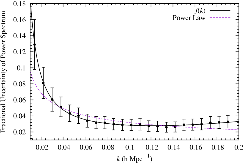
Figure 4 shows a similar plot for the off-diagonal elements of the reduced covariance matrix, where we plotted the measurements in terms of $\Delta k$. Our fitting function seems to provide a good phenomenological description of this function. We find that reducing the number of parameters by eliminating either the sinc term (by setting $\alpha=1$) or the $\beta$ term (by setting $\beta=0$) significantly worsens the fit.

Figure 4: The independent off-diagonal elements of the correlation matrix plotted as a function of $\Delta k$. Grey data points represent individual $r_{ij}$ elements while the black data points are the weighted mean and variance for the elements with the same value of $k_{i}-k_{j}$. Our proposed function, $g(\Delta k)$, seems to fit quite well for the full range of $\Delta k$ ($\chi^{2}=219.6$, $N_{\mathrm{DoF}}=249$). The best-fits for the Lorentzian plus constant term and Lorentzian plus sinc term result in noticeably worse fits ($\chi^{2}=252.9$, $N_{\mathrm{DoF}}=251$ and $\chi^{2}=388.7$, $N_{\mathrm{DoF}}=250$, respectively). Note that the terms of each fitted function are combined in such a way as to enforce that they are equal to one when $\Delta k=0$.

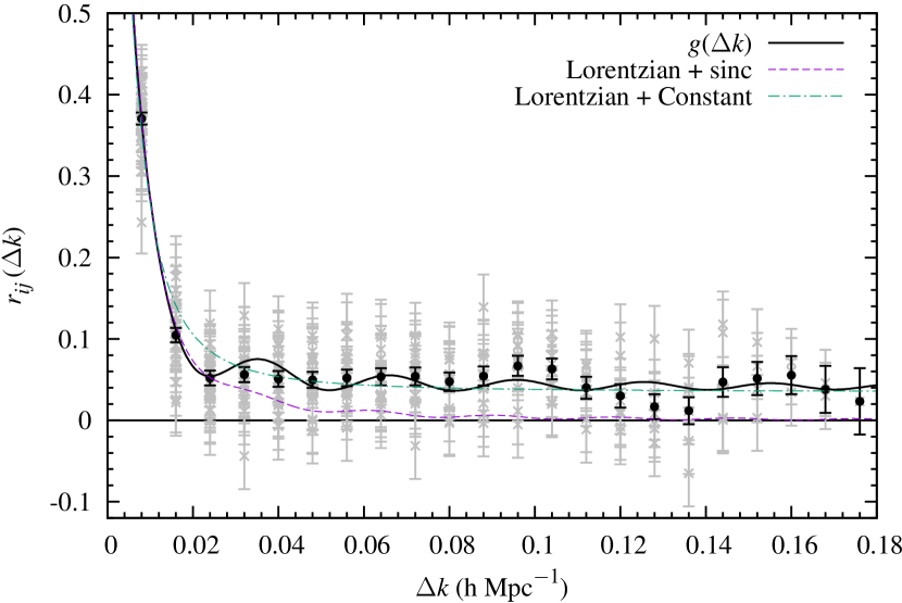
After performing the full fit to all independent covariance matrix elements we get $a=(451\pm 35)h^{-1}\mathrm{Mpc}$, $b=-1.19\pm 0.02$, $\nu=(9.62\pm 0.32)h^{-1}\mathrm{Mpc}$, $\alpha=0.867\pm 0.024$, $\gamma=(5.17\pm 0.16)\times 10^{-3}h~{}\mathrm{Mpc}^{-1}$, $\omega=(211.35\pm 6.14)h^{-1}\mathrm{Mpc}$, and $\beta=0.0423\pm 0.0033$, with $\chi^{2}=250.6$ for 269 degrees of freedom. The best-fitting value for $\omega$ is close to the theoretically expected value of the average depth of the survey divided by $2\pi$.

5 Convergence of the covariance matrix

The main advantage of the fitting function approach is that the covariance matrix elements converge to their true values much faster than the sample variance. Figure 5 shows the offset of individual covariance (and inverse covariance) matrix elements estimated using sample variance (light blue points) and our method (purple points) as the number of mocks increases. The offset is normalized to the standard deviation from the final ($N=600$) covariance (and inverse covariance) matrix given by Eqs. (10) and (11) (or Eqs. (15) and (16) for the inverse). The fitting function method converges to the final result much faster both for the covariance and inverse covariance matrices.

Figure 5: Convergence of the covariance (top) and inverse covariance (bottom) matrices to their final values (computed using 600 mocks) with the number of mocks. The light blue points show the matrices determined from the mock catalogs in the standard way, while the purple dots show the matrices as determined using our fitting function. It is clear that the matrices from the best-fitting functions converge much faster than the ones determined from sample variance. See the online article for the colour version of this plot.

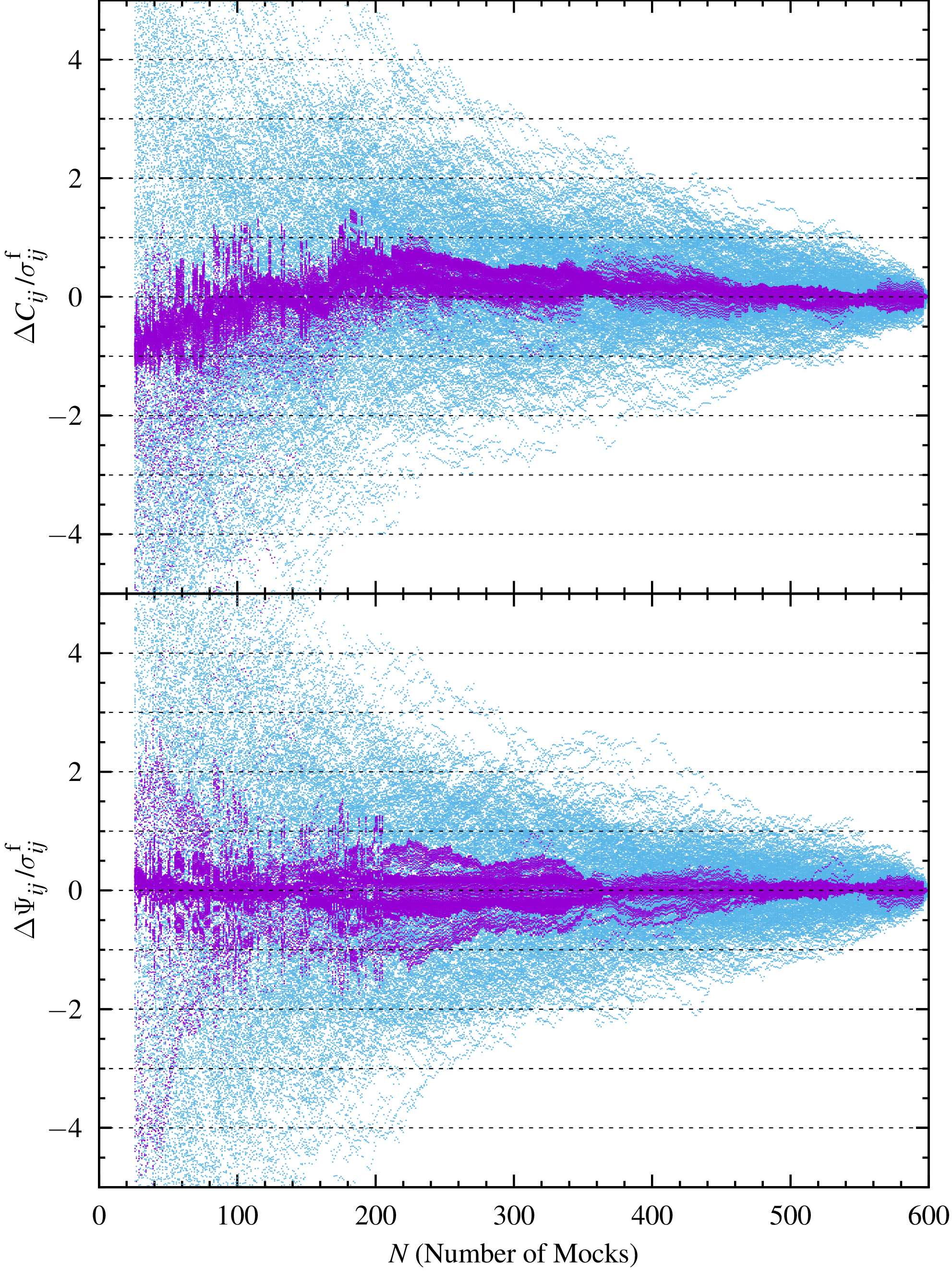
Figure 6 shows a histogram of the distribution of estimated $C_{ij}$ elements around their true value for $N=50$. This is a horizontal slice of the top panel of Figure 5. Already, very few elements estimated with the fitting function method are outside 3$\sigma$ of the true covariance, while for the sample variance method the distribution is basically flat.

Figure 6: Histograms of the differences between intermediate (generated using first 50 mocks) covariance matrices and the final (using all 600 mocks) covariance matrix normalized by the uncertainty in the final sample covariance matrix. While slightly biased, the fitting functions already provide a significantly better approximation of the final covariance matrix.

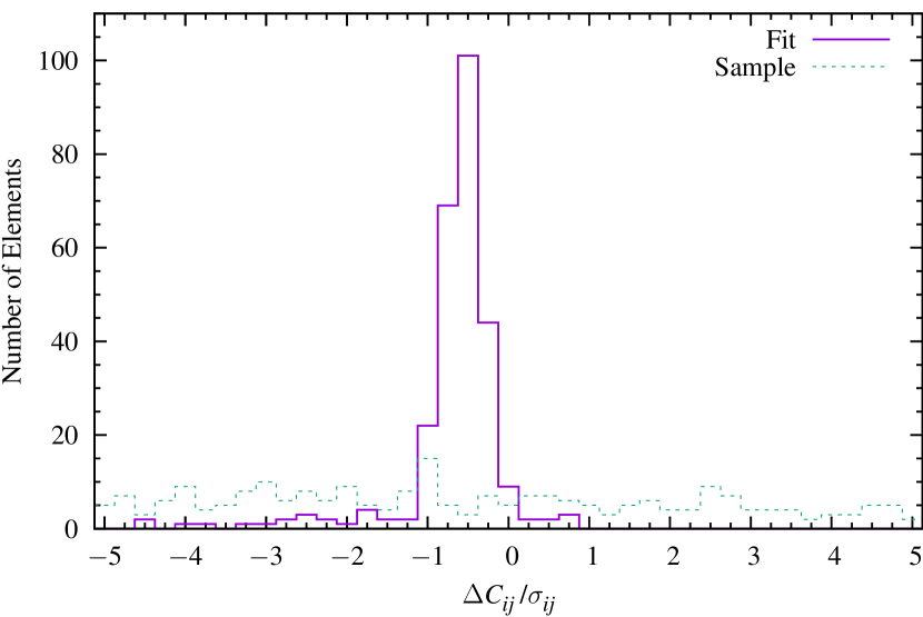
At low $N$, there is a small bias in $C_{ij}$ elements determined from the fitting function method but it’s significantly smaller than the variance in $C_{ij}$-s determined from the sample variance and therefore the fitting function method is still superior.

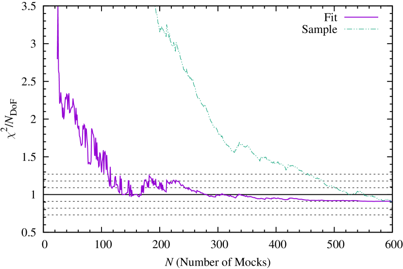
Figure 7 shows the convergence to the final covariance in terms of $\chi^{2}$ per degree of freedom (DoF) for the two methods. Since the final covariance matrices computed with fitting function and sample variance methods are close to each other in $\chi^{2}$, either one of them can be treated as a good approximation for the true covariance matrix. To put both methods on equal footing, when computing the $\chi^{2}$ for the fitting function method we compare it to the final ($N=600$) sample variance method and vice versa. Figure 7 clearly demonstrates that the fitting function method generated $C_{ij}$-s become consistent with the true covariance matrix much faster (already at $N\sim 100$) compared to those generated from the sample variance.

Figure 7: Reduced $\chi^{2}$ of the covariance matrix compared to the final covariance. The solid line is for the results obtained using the fitting function and the dot-dashed line is for the sample covariance matrix. Horizontal dashed lines show the expected 1, 2, and 3$\sigma$ deviations from the $\chi^{2}/N_{\mathrm{DoF}}=1$ line.

6 Conclusions

We propose a new method of estimating the elements of the covariance matrix for band-averaged $P(k)$ measurements from galaxy surveys. The essence of the method is to find a fitting function for the covariance matrix and calibrate its parameters using a sample covariance computed from a set of mock catalogues. We show that for the $P(k)$ measurements from the BOSS DR11 data in the range of $0\leq k\leq 0.2h~{}\mathrm{Mpc}^{-1}$ a very simple, seven-parameter function, given by Eq. (21), is sufficient to describe the covariance matrix. The fitting function covariance matrix is statistically indistinguishable from the sample covariance matrix computed from 600 mocks catalogues.

The greatest advantage of this method, compared to the standard method of using the sample covariance matrix, is that it requires significantly fewer mock catalogues for calibration to converge to the true covariance matrix (see figure 5). For the BOSS DR11 data, the fitting function generated covariance matrices calibrated with as few as $\sim$100 mocks were statistically indistinguishable from the sample covariance matrix generated with 600 mocks. To get a similar convergence with the sample covariance matrix we had to use more than 400 mocks (see figure 7). This advantage of the new method is especially relevant in situations where only a few mock catalogues are available. With only 50 mock catalogues the distribution of the sample covariance around the true value is basically flat, while the fitting function method already provides a decent approximation (see figure 6).

The specific functional form that we tested in this work may turn out to be an approximation that is too crude for future surveys, which will demand much higher accuracy on the determination of $C_{ij}$. The functional form may have to be modified if one wishes to include $P(k)$ measurements on much smaller scales as well. However, once an appropriate (for the sought precision) functional form is found, there is no reason why this method should not work with future data.

In future work we plan to study how this new method works at higher precision. The uncertainties in the elements of the sample covariance (and inverse sample covariance) matrix scale inversely with the number of mocks (see seciont 3). A larger suite of mock catalogues would enable us to better estimate the true covariance (and inverse covariance) matrix with much smaller error bars on its elements. This would allow us to determine what modifications of our fitting function are required at higher precision to model the true covariance matrix. This would have the additional benefit of testing the fitting function method against a set of mocks which is completely independent from the set used in this work, ruling out the possibility that our successes were the result of some peculiarity which may be present in the data.

This work was concerned only with the band-averaged $P(k)$. Higher order Legendre polynomials of $P(k)$ with respect to the line-of-sight provide valuable information about the nature of gravity and the expansion rate. The measurement of various Legendre moments of $P(k)$ will be cross-correlated. We will address the question of modelling this larger covariance (and inverse covariance) matrix in future work as well.

References

- Anderson (2003) Anderson T. W., 2003, Introduction to Multivariate Statistical Analysis
- Anderson et al. (2014) Anderson L., et al., 2014, MNRAS, 441, 24
- Bernardeau et al. (2002) Bernardeau F., Colombi S., Gaztañaga E., Scoccimarro R., 2002, Phys. Rep., 367, 1
- Beutler et al. (2011) Beutler F., et al., 2011, MNRAS, 416, 3017
- Chuang et al. (2015) Chuang C.-H., et al., 2015, MNRAS, 452, 686
- Cole et al. (2005) Cole S., et al., 2005, MNRAS, 362, 505
- Coles & Jones (1991) Coles P., Jones B., 1991, MNRAS, 248, 1
- Dawson et al. (2013) Dawson K. S., et al., 2013, AJ, 145, 10
- Dodelson & Schneider (2013) Dodelson S., Schneider M. D., 2013, Phys. Rev. D, 88, 063537
- Eisenstein et al. (2011) Eisenstein D. J., et al., 2011, AJ, 142, 72
- Feldman et al. (1994) Feldman H. A., Kaiser N., Peacock J. A., 1994, ApJ, 426, 23
- Frieman & Dark Energy Survey Collaboration (2013) Frieman J., Dark Energy Survey Collaboration 2013, in American Astronomical Society Meeting Abstracts 221. p. 335.01
- Gil-Marín et al. (2015) Gil-Marín H., Noreña J., Verde L., Percival W. J., Wagner C., Manera M., Schneider D. P., 2015, MNRAS, 451, 5058
- Hamilton et al. (2006) Hamilton A. J. S., Rimes C. D., Scoccimarro R., 2006, MNRAS, 371, 1188
- Hartlap et al. (2007) Hartlap J., Simon P., Schneider P., 2007, A&A, 464, 399
- Kitaura et al. (2014) Kitaura F.-S., Yepes G., Prada F., 2014, MNRAS, 439, L21
- Kitaura et al. (2015) Kitaura F.-S., Gil-Marín H., Scóccola C. G., Chuang C.-H., Müller V., Yepes G., Prada F., 2015, MNRAS, 450, 1836
- LSST Science Collaboration et al. (2009) LSST Science Collaboration et al., 2009, preprint, (arXiv:0912.0201)
- Laureijs et al. (2011) Laureijs R., et al., 2011, preprint, (arXiv:1110.3193)
- Levi et al. (2013) Levi M., et al., 2013, preprint, (arXiv:1308.0847)
- Manera et al. (2013) Manera M., et al., 2013, MNRAS, 428, 1036
- Manera et al. (2015) Manera M., et al., 2015, MNRAS, 447, 437
- Meiksin & White (1999) Meiksin A., White M., 1999, MNRAS, 308, 1179
- Monaco et al. (2002) Monaco P., Theuns T., Taffoni G., 2002, MNRAS, 331, 587
- Monaco et al. (2013) Monaco P., Sefusatti E., Borgani S., Crocce M., Fosalba P., Sheth R. K., Theuns T., 2013, MNRAS, 433, 2389
- Norberg et al. (2009) Norberg P., Baugh C. M., Gaztañaga E., Croton D. J., 2009, MNRAS, 396, 19
- Paz & Sanchez (2015) Paz D. J., Sanchez A. G., 2015, preprint, (arXiv:1508.03162)
- Percival et al. (2014) Percival W. J., et al., 2014, MNRAS, 439, 2531
- Pope & Szapudi (2008) Pope A. C., Szapudi I., 2008, MNRAS, 389, 766
- Reid et al. (2010) Reid B. A., et al., 2010, MNRAS, 404, 60
- Rimes & Hamilton (2006) Rimes C. D., Hamilton A. J. S., 2006, MNRAS, 371, 1205
- Schlegel et al. (2009) Schlegel D. J., et al., 2009, preprint, (arXiv:0904.0468)
- Schlegel et al. (2011) Schlegel D., et al., 2011, preprint, (arXiv:1106.1706)
- Schneider et al. (2011) Schneider M. D., Cole S., Frenk C. S., Szapudi I., 2011, ApJ, 737, 11
- Scoccimarro & Frieman (1999) Scoccimarro R., Frieman J. A., 1999, ApJ, 520, 35
- Scoccimarro & Sheth (2002) Scoccimarro R., Sheth R. K., 2002, MNRAS, 329, 629
- Scoccimarro et al. (1999) Scoccimarro R., Zaldarriaga M., Hui L., 1999, ApJ, 527, 1
- Sefusatti & Scoccimarro (2005) Sefusatti E., Scoccimarro R., 2005, Phys. Rev. D, 71, 063001
- Sefusatti et al. (2006) Sefusatti E., Crocce M., Pueblas S., Scoccimarro R., 2006, Phys. Rev. D, 74, 023522
- Sirko (2005) Sirko E., 2005, ApJ, 634, 728
- Takahashi et al. (2009) Takahashi R., et al., 2009, ApJ, 700, 479
- Tassev et al. (2013) Tassev S., Zaldarriaga M., Eisenstein D. J., 2013, J. Cosmology Astropart. Phys., 6, 36
- Taylor & Joachimi (2014) Taylor A., Joachimi B., 2014, MNRAS, 442, 2728
- Taylor et al. (2013) Taylor A., Joachimi B., Kitching T., 2013, MNRAS, 432, 1928
- Tegmark (1997) Tegmark M., 1997, Physical Review Letters, 79, 3806
- White et al. (2014) White M., Tinker J. L., McBride C. K., 2014, MNRAS, 437, 2594
- Xu et al. (2012) Xu X., Padmanabhan N., Eisenstein D. J., Mehta K. T., Cuesta A. J., 2012, MNRAS, 427, 2146
- de Putter et al. (2012) de Putter R., Wagner C., Mena O., Verde L., Percival W. J., 2012, J. Cosmology Astropart. Phys., 4, 19
- de la Torre et al. (2013) de la Torre S., et al., 2013, A&A, 557, A54