Saddle point inflation from higher order corrections to Higgs/Starobinsky inflation
Abstract
We explore two saddle point inflationary scenarios in the context of higher order corrections related to different generalisations of general relativity. Firstly, we deal with Jordan frame Starobinsky potential, for which we identify a portion of a parameter space of inflection point inflation, which can accommodate all the experimental results. Secondly, we analyse Higgs inflation and more specifically the influence of non-renormalisible terms on the standard quartic potential. All results were verified with the PLANCK 2015 data.
I Introduction
Cosmic inflation Lyth:1998xn ; Liddle:2000dt ; Mazumdar:2010sa is a theory of the early universe which predicts cosmic acceleration and generation of seeds of the large scale structure of the present universe. It solves problems of classical cosmology and it is consistent with current experimental data Ade:2013uln . It is instructive to study minimal models of inflation which have the form of small modifications of the canonical models describing features of the visible Universe. Two most prominent examples of such models are, at the moment, theories of gravity models of Higgs inflation.
The first theory of inflation was the Starobinsky model Starobinsky:1980te ; Barrow:1988xh , which is an theory DeFelice:2010aj with Lagrangian density. In such a model the acceleration of space-time is generated by the gravitational interaction itself, without a need to introduce any new particles or fields. The embedding of Starobinsky inflation in no-scale SUGRA has been discussed in Ref. Ellis:2015xna . The Starobinsky inflation can be described as a special case of the Brans-Dicke theory Brans:1961sx and its predictions are consistent with the so-called Higgs inflation Bezrukov:2007ep , in which inflation is generated by the scalar field non-minimally coupled to gravity. Recently the whole class of generalisations of the Starobinsky and Higgs inflation have been discussed in the literature Codello:2014sua ; Ben-Dayan:2014isa ; Artymowski:2014gea ; Artymowski:2014nva ; Sebastiani:2013eqa ; Motohashi:2014tra ; Salvio:2015kka ; Hamada:2014wna , also in the context of the higher order terms in Starobinsky Jordan frame potential Broy:2014sia ; Kamada:2014gma ; Artymowski:2015mva .
On the other hand, Higgs inflation allows one to generate inflation close to the Higgs sector. The price is the non-minimal coupling to gravity and often additional interactions which allow one to reproduce all features of realistic inflationary scenarios. In particular, corrections to the model can often be represented by higher order scalar operators. This reminds one of the situation known from theories, where higher order corrections to the f(R) function seem to be unavoidable. Usually one assumes that there is a part of the Starobinsky/Higgs inflationary potential where higher order terms are subdominant, which creates an inflationary plateau long enough to support successful inflation. Nevertheless one can find a part of parameter space where higher order corrections give significant contribution to the potential for relatively small values of field, which makes the plateau region too short to generate cosmic inflation with at least 60 e-foldings. In this case a saddle point inflation generated by the higher order terms may be the only chance to obtain a successful inflationary model, which is the issue we investigate in this paper.
In Artymowski:2015mva we proved that the Starobinsky potential with higher order corrections (i.e. higher powers of the Jordan frame Starobisnky potential) can have a saddle point for some on the plateau. This requires a certain relation between parameters of the model and leads to the existence of the Starobinsky plateau, a step slope of exponential potential and a saddle point in between. In this paper we perform the detailed analysis of such a model in the context of low-scale inflation and generation of primordial inhomogeneities, especially in the context of very big values of higher order terms. We apply the same approach to the Higgs inflation. In this case the motivation is even more natural: higher order corrections to the scalar potential (such as or , where is a scalar field, but not necessarily the Higgs field itself) are considered to be suppressed by the Planck scale. Consequently for sufficiently high values of field one has to take into account the influence of higher order terms. In particular higher order terms coefficients could be fine-tuned to create a saddle point (or deflation point) in the Einstein frame scalar potential. In Ref Artymowski:2015pna we have also investigated the saddle-point inflation in theory generated by higher order corrections to the Starobinsky model. Note that in this paper we investigate the issue of higher order corrections to Jordan frame scalar potentials, not to the function itself.
In what follows we use the convention , where is the reduced Planck mass.
The outline of the paper is as follows. In Sec. II we introduce the form of the potential in modified Strobinsky case and we analyse its features. In Sec. III we analyse the saddle point inflation in this model and the evolution of primordial inhomogeneities. In Sec IV we investigate the saddle point within the Higgs inflation scenario. Finally, we conclude in Sec. V.
II Starobinsky-like potential with a saddle point
II.1 Jordan frame analysis
Let us consider a Brans-Dicke theory in the flat FRW space-time with the metric tensor of the form . Any theory can be expressed in terms of the auxiliary field with the Jordan frame scalar potential . The Jordan frame action is of the form
| (II.1) |
where is the action of matter fields. In the context of inflation one can assume that the energy density of the universe is fully dominated by the inflaton, which gives . Then, for the homogeneous field the field’s equation of motion and the first Friedmann equation become DeFelice:2010aj
| (II.2) | |||||
| (II.3) |
where . Let us note that for one recovers general relativity (GR). Thus the will be denoted as the GR vacuum.
The Starobinsky inflation is a theory of cosmic inflation based on the action, which can be generalized into Brans-Dicke theory with general value of . The Jordan frame potential of the Starobinsky model takes the following form
| (II.4) |
where is a mass parameter, and its value comes from the normalisation of the primordial inhomogeneities. For one finds . The Starobinsky potential is presented in Fig. 1. In this paper we consider the extension of this model motivated by Ref. Broy:2014sia and partially analysed in Ref. Artymowski:2015mva , namely
| (II.5) |
where , are numerical coefficients. In order to avoid for we assume that . We want to keep terms as higher order corrections (i.e. we want to remain in perturbative regime of the theory), thus we require and . As we will show the assumed range of parameters will satisfy these conditions.
II.2 Einstein frame analysis
The gravitational part of the action may obtain its canonical (minimally coupled to ) form after transformation to the Einstein frame. Let us assume that . Then for the Einstein frame metric tensor
| (II.6) |
one obtains the action of the form of
| (II.7) |
where is the derivative with respect to the Einstein frame coordinates, , at and is the Ricci scalar of . The GR vacuum appears for . Let us define the Einstein frame Hubble parameter as
| (II.8) |
Then for the first Friedmann equation and the equation of motion of are following
| (II.9) |
where .
II.3 Saddle point of the Einstein frame potential
In Ref. Artymowski:2015mva we showed that the Einstein frame potential of the model from Eq. (II.5) has a saddle point at for , where
| (II.10) |
where . Let us note that for one obtains a saddle point inflation, which in principle could significantly decrease the scale of inflation. For the term is always subdominant as compared to the other terms of and it can be neglected in the analysis. Therefore, the potential has no stationary points besides the minimum at . On the other hand, for one obtains a potential with a local maximum at the plateau, step slope for big and a minimum in between. This case was analysed in Artymowski:2015mva . The Eq. II.10 gives approximate value of and , but it predicts all derivatives of for and to be of order of . This is not consistent with the saddle-like point condition and therefore Eq. II.10 is not accurate enough to calculate power spectra of primordial inhomogeneities.
The analysis presented in this subsection is done under several assumptions and approximations and therefore its accuracy is limited by them. For instance one finds and . We have assumed that and we have obtained . Thus, the assumption is satisfied for , which is also the condition for . One can see that the approximation used in this subsection is far more accurate for the condition than for the condition.
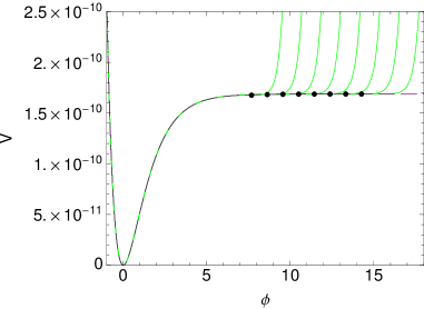
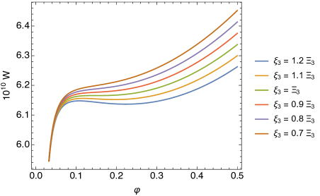
III Inflationary dynamics and primordial inhomogeneities
III.1 Inflation with and beyond the slow-roll approximation
In this section we will discuss the slow-roll approximation and inflation in the Einstein frame. We want to investigate how non-zero values of parameters deviate the inflation from the Starobinsky model. Let us assume that . Then one obtains
| (III.1) |
This approximation holds for non-zero values of , so one cannot use Eq. (III.1) at . Thus we will use the slow-roll equations for . The cosmic inflation takes place as long as following slow-roll parameters are much smaller than one
| (III.2) |
The number of e-folds generated during the inflation is in the slow-roll approximation equal to
| (III.3) |
where indexes and refer to initial and final moments of inflation respectively. Namely, is the first moment when both slow-roll parameters are smaller than one and is the moment when any of slow-roll parameters become bigger than one. In Fig. 6 of Ref. Artymowski:2015mva we showed that during the saddle-point inflation it is straightforward to generate the number of e-folds significantly bigger than 60, even if the plateau is not present at all.
The power spectra of the superhorizon primordial curvature perturbations and gravitational waves in the Einstein frame are following
| (III.4) |
The needs to be normalized at the horizon crossing of scales observed in the CMB. Usually one chooses the normalization moment to be at (where the denotes the value of the quantity at the horizon crossing), but in general the scale of normalisation strongly depends on the scale of inflation and reheating. In this paper we set , where is the Fourier mode of perturbation, and . The value of decreases for big , since for lower scale of inflation the comoving Hubble radius will grow less during the post-inflationary era. This procedure sets .
We have several parameters in the model, namely , , , and , however since we require the existence of the saddle point, one finds and . From its definition depends on , and . The normalization is a constraint which we use to calculate required , thus decreasing the amount of free parameters to just . We will use to parametrise the deviation from the Starobinsky inflation.
Two parameters of power spectra, which connect theory with the experiment are the tensor to scalar ratio and the scalar spectral index defined by
| (III.5) |
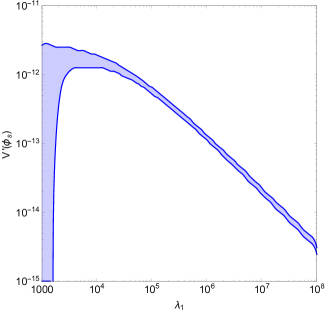
where is the Fourier mode. In the saddle point inflation one expects , so and . Since is excluded by the experimental data Ade:2013uln one needs at the moment of freeze-out. Thus, one requires . The total amount of e-folds produced for strongly depends on the length of the Starobinsky plateau and therefore on . If the plateau for is long enough to generate at least e-folds of inflation then the does not significantly deviate from the Starobinsky one. On the other hand for one may decrease the length of the plateau in order to generate e-folds only via the saddle point inflation. As we will show, this may be the way to decrease and therefore to obtain the low-scale inflation.
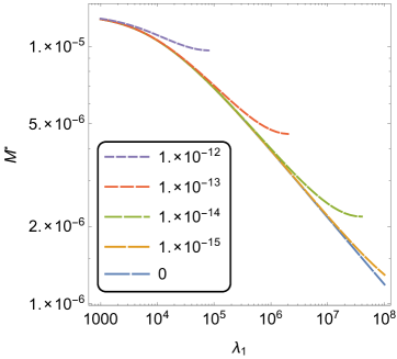
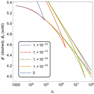
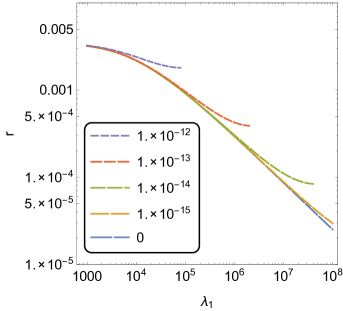
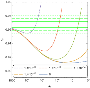
In Fig. 2 we present , and as a function of . One can see that for the decreases logarithmically with to reach at . For the normalisation of inhomogeneities happens very close to . Nevertheless, for all considered values of we obtained . In Fig. 3 we present and for . For (i.e. for a perfect saddle) and for one finds and the model becomes inconsistent with the PLANCK data. The perfect saddle may still fit the data for , however then inflation simply occurs on the plateau far from the saddle and the whole modification is simply irrelevant. Thus let us consider the case of to check if the inflection point inflation gives the correct values of . The value of the field at the inflection will also be denoted as . The results of numerical analysis for saddle and inflection point inflation for different and are presented in Fig. 2 and 3. For the inflection point inflation one finds the maximal allowed for which the number of e-folds generated for is equal to , which is the number of e-folds at the horizon crossing for the normalisation scale .
The key result is that inflection point inflation satisfies experimental constraints even for large values of . This means that it remains a valid solution, and one is not limited to very small modifications of the potential which would simply mean going back to the Starobinsky model. This unfortunately is not true for the pure saddle case in which inflation has to occur on the plateau and the potential can only be modified for very large field values.
IV Saddle point Higgs inflation
The saddle point inflation can be also obtained from higher order corrections to the so-called Higgs inflation. Let us define the action of a real scalar field (which in particular may be a Higgs field) with non-minimal coupling to gravity as
| (IV.1) |
where is the Jordan frame scalar potential, is the Ricci scalar, is the function of non-minimal coupling to the gravity and is the action of matter fields, like dust, radiation, additional scalar fields etc. We assume that all fields in are minimally coupled to gravity. For one restores general relativity. In further parts of this section we will assume that
| (IV.2) |
where . Thus, the limit gives the GR vacuum. In the model the slow-roll parameters are proportional to , so inflation happens for . Let us assume that is of the form
| (IV.3) |
where and is a scalar potential which corresponds to the high energy approximation of the Mexican hat potential used e.g. to describe self-interaction of the Higgs field. Terms proportional to and are the higher order corrections to this potential 111The issue of saddle point Higgs inflation without higher order corrections has been partially analysed in Ref Bezrukov:2014bra .. The constants are dimensionless. As we will show one need to require in order to obtain positive energy density and stability of the potential at very high energies. Nevertheless the sign of remains undetermined.
In order to obtain the canonical form of the action let us consider the transformation to the Einstein frame, namely
| (IV.4) | |||||
| (IV.5) |
where is the Einstein frame field and is the Einstein frame potential. For one finds , which is the result from the Brans-Dicke theory. The potential for several values of and parameters has been presented in Fig. 1. Let us note that for one restores the potential from Ref. Bezrukov:2007ep . Now the equations of motion take the form
| (IV.6) |
where and . The potential has a minimum at , which corresponds to the GR limit of the theory. In the , approximation one finds following analytical relations, which determine the existence of the saddle point in the Einstein frame
| (IV.7) |
For the potential has a minimum at and flat plateaus, which ends with step, exponential slopes. The potential is always growing with and one finds no stationary points. For the only stationary points besides the minimum at are two saddle points at . For the potential has additional minima and maxima at some and respectively.
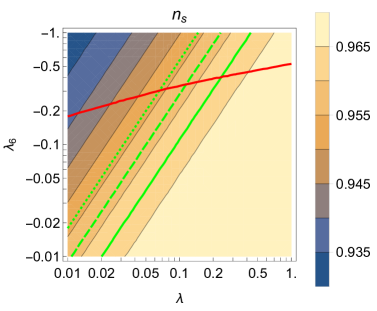
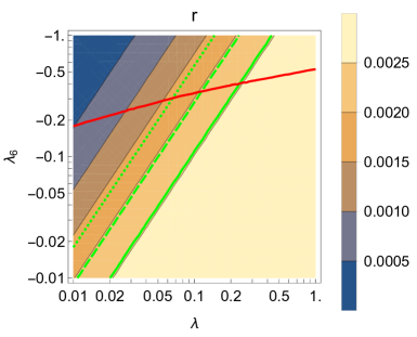
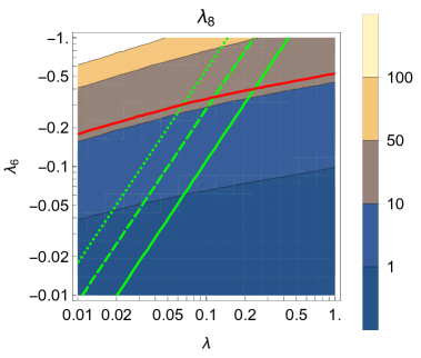
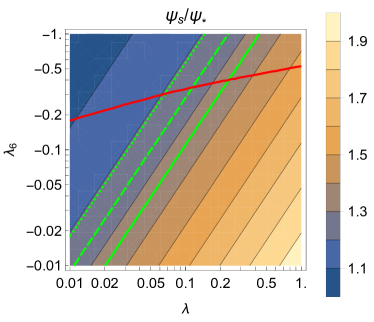
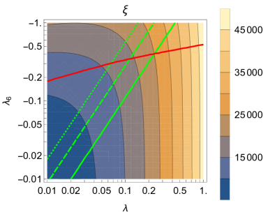
We start from 5 free parameters: , , , and . We have 3 constraints: , and , which we use to determine , and . In Fig. 5 we show the and dependence of , , and . In Fig. 6 we show weak dependence of in the allowed part of the parameter space. The parameter is naturally limited by . In order to preserve perturbativity of the theory let us assume that and should not be bigger than . It is crucial that even including all these constraints a significant part of the parameter space remains valid. Even though inflation occurs some distance away from the saddle () and so some influence of the plateau is inevitable, such an extension remains a viable extension of the standard Higgs inflation scenario.
V Conclusions
In this paper we investigated the possibility of generating saddle point inflation from higher order corrections to theories of modified gravity, namely the Starobinsky model and Higgs inflation. It is crucial that even after including all constraints we discussed, a large portion of the parameter space in both models remains valid. Even though in modified Higgs inflation scenario and Starobinsky model with a pure saddle, inflation has to occur some distance away from the saddle to achieve correct values of , and so some influence of the plateau is inevitable. Inflection or saddle point inflation remain a viable extension of the standard Starobinsky model and Higgs inflation scenarios.
The significant difference between the two is the number of free parameters which in the Higgs inflation case allows solutions with pure saddle to be consistent with all constraints. On the contrary, in modification of the Starobinsky model we had to resort to inflection point inflation rather than a pure saddle in order to achieve new valid results. Note that higher order corrections do not change the position of Einstein frame vacuum and therefore they do not change the consistency between GR and low energy predictions of discussed theories.
In Sec. II we introduced higher order corrections to the Jordan frame potential of the Starobinsky theory. We presented the analytical analysis of the existence of the saddle point of the Einstein frame potential.
In Sec. III we analyse features of primordial inhomogeneities generated during saddle point inflation. From the normalisation of perturbations and saddle (inflection) point conditions we obtained all parameters of the model (such as , , and ) as functions of . We found the region in the space which fits the regime of PLANCK. We showed how (and therefore the scale of inflation) can decrease for big and we estimated the maximal allowed value of to be of order of . The inflation can happen almost exactly at the inflection point and no Starobinsky plateau is needed to obtain correct shape of the power spectrum. For consistency with PLANCK can be obtained even for . In such a case one obtains the Starobinsky plateau for , which has significant influence on the generation of primordial inhomogeneities during the last 60 e-folds of inflation.
In Sec. IV we investigated the issue of higher order corrections to the potential. We found conditions for the existence of a saddle point as well as constrains in the plane, which come from perturbativity of the theory and consistency with PLANCK. The result is that the saddle point inflation is possible in such a model. However during the last 60 e-folds of inflation, interesting part of the potential is also influenced by the term, which generates Starobinsky-like plateau. This comes from the fact that in the allowed region of parameters , which means that inflation has to proceed on the plateau some distance from the saddle, in order to satisfy experimental constraints.
Acknowledgements
This work was partially supported by the Foundation for Polish Science International PhD Projects Programme co-financed by the EU European Regional Development Fund and by National Science Centre under research grants DEC-2012/04/A/ST2/00099 and DEC-2014/13/N/ST2/02712. ML was supported by the Polish National Science Centre under doctoral scholarship number 2015/16/T/ST2/00527. MA was supported by National Science Centre grant FUGA UMO-2014/12/S/ST2/00243.
References
- (1) D. H. Lyth and A. Riotto, Phys. Rept. 314 (1999) 1 [hep-ph/9807278].
- (2) A. R. Liddle, New Astron. Rev. 45 (2001) 235 [astro-ph/0009491].
- (3) A. Mazumdar and J. Rocher, Phys. Rept. 497 (2011) 85 [arXiv:1001.0993 [hep-ph]].
- (4) P. A. R. Ade et al. [Planck Collaboration], Astron. Astrophys. 571 (2014) A22 [arXiv:1303.5082 [astro-ph.CO]].
- (5) A. A. Starobinsky, Phys. Lett. B 91 (1980) 99.
- (6) J. D. Barrow and S. Cotsakis, Phys. Lett. B 214 (1988) 515.
- (7) A. De Felice and S. Tsujikawa, Living Rev. Rel. 13 (2010) 3 [arXiv:1002.4928 [gr-qc]].
- (8) J. Ellis, M. A. G. Garcia, D. V. Nanopoulos and K. A. Olive, arXiv:1507.02308 [hep-ph].
- (9) C. Brans and R. H. Dicke, Phys. Rev. 124 (1961) 925.
- (10) F. L. Bezrukov and M. Shaposhnikov, Phys. Lett. B 659 (2008) 703 [arXiv:0710.3755 [hep-th]].
- (11) A. Codello, J. Joergensen, F. Sannino and O. Svendsen, arXiv:1404.3558 [hep-ph].
- (12) I. Ben-Dayan, S. Jing, M. Torabian, A. Westphal and L. Zarate, arXiv:1404.7349 [hep-th].
- (13) M. Artymowski and Z. Lalak, JCAP09(2014)036 [arXiv:1405.7818 [hep-th]].
- (14) M. Artymowski, Z. Lalak and M. Lewicki, arXiv:1412.8075 [hep-th].
- (15) L. Sebastiani, G. Cognola, R. Myrzakulov, S. D. Odintsov and S. Zerbini, Phys. Rev. D 89 (2014) 023518 [arXiv:1311.0744 [gr-qc]].
- (16) H. Motohashi, arXiv:1411.2972 [astro-ph.CO].
- (17) A. Salvio and A. Mazumdar, Phys. Lett. B 750 (2015) 194 [arXiv:1506.07520 [hep-ph]].
- (18) Y. Hamada, H. Kawai, K. y. Oda and S. C. Park, Phys. Rev. D 91 (2015) 053008 [arXiv:1408.4864 [hep-ph]].
- (19) B. J. Broy, D. Roest and A. Westphal, arXiv:1408.5904 [hep-th].
- (20) K. Kamada and J. Yokoyama, Phys. Rev. D 90 (2014) 10, 103520 [arXiv:1405.6732 [hep-th]].
- (21) M. Artymowski, Z. Lalak and M. Lewicki, JCAP 1506 (2015) 06, 032 [arXiv:1502.01371 [hep-th]].
- (22) M. Artymowski, Z. Lalak and M. Lewicki, Phys. Lett. B 750 (2015) 595 doi:10.1016/j.physletb.2015.09.076 [arXiv:1508.05150 [gr-qc]].
- (23) F. Bezrukov and M. Shaposhnikov, Phys. Lett. B 734 (2014) 249 doi:10.1016/j.physletb.2014.05.074 [arXiv:1403.6078 [hep-ph]].