Schramm-Loewner Evolution and isoheight lines of correlated landscapes

Abstract

Real landscapes are usually characterized by long-range height-height correlations, which are quantified by the Hurst exponent $H$. We analyze the statistical properties of the isoheight lines for correlated landscapes of $H\in[-1,1]$. We show numerically that, for $H\leq 0$ the statistics of these lines is compatible with $SLE$ and that established analytic results are recovered for $H=-1$ and $H=0$. This result suggests that for negative $H$, in spite of the long-range nature of correlations, the statistics of isolines is fully encoded in a Brownian motion with a single parameter in the continuum limit. By contrast, for positive $H$ we find that the one-dimensional time series encoding the isoheight lines is not Markovian and therefore not consistent with $SLE$.

We study isoheight lines of long-range correlated landscapes. They are the paths of constant height in topography Boffetta et al. (2008), the equipotential lines on energy landscapes Ziman (1968); Weinrib (1982), and the constant vorticity lines in turbulent vorticity fields Bernard et al. (2006). Empirical and numerical studies of isoheight lines show that they are usually scale invariant Mandelbrot (1983); Kondev and Henley (1995) and that their fractal dimension $d_{f}$ depends on the long-range correlations, quantified by the Hurst exponent $H$ Schrenk et al. (2013).

One solid framework to study fractal curves in two-dimensions is the Schramm-Loewner Evolution ($SLE$) theory Schramm (2000). Accordingly, an $SLE$ curve can be mapped onto a one-dimensional Brownian motion of a single parameter in the continuum limit. Establishing that isoheight lines are $SLE$ would allow us to generate an ensemble of such curves by simply solving a stochastic differential equation, without generating the entire landscape, and to extend established results from $SLE$ to isoheight lines.

We analyze the zero isoheight lines of random surfaces of different $H$ generated with free boundary conditions on a triangular lattice of size $L_{x}\times L_{y}$ with $L_{x}>L_{y}$. We consider chordal curves that are non-self-touching curves growing to infinity in the upper half-plane $\mathbb{H}$, starting at the origin. From the Riemann mapping theorem, there is a unique conformal map $g_{t}$ that iteratively maps the complement of such a curve in the upper half-plane $\mathbb{H}$ back onto $\mathbb{H}$. This map satisfies the Loewner differential equation,

$$\frac{\partial g_{t}(z)}{\partial t}=\frac{2}{g_{t}(z)-\xi_{t}},$$ (1)

with $g_{0}(z)=z$ and $\xi_{t}$ a real continuous function, called the driving function. If a curve is $SLE_{\kappa}$ then $\xi_{t}=\sqrt{\kappa}B_{t}$, where $B_{t}$ is a standard one-dimensional Brownian motion and $\kappa$ is the diffusion constant. We show that, while for $H\leq 0$ the statistics of $\xi_{t}$ is consistent with a Brownian motion, for $H>0$, $\xi_{t}$ is not Markovian and therefore $SLE$ cannot be established.

We generate random landscapes on a triangular lattice, by assigning to each lattice site $\mathbf{x}=(x,y)$ a random height $h(\mathbf{x})$, imposing long-range correlations with the following spectrum,

$$S(\mathbf{q})\sim|\mathbf{q}|^{-\beta_{c}}\ \ ,$$ (2)

where $\beta_{c}=2(H+1)$ and $H$ is the Hurst exponent. For that, we use the Fourier Filtering Method Prakash et al. (1992); Makse et al. (1996); Ahrens and Hartmann (2011) where,

$$h\left(\mathbf{x}\right)=\tilde{\mathcal{F}}\left(\sqrt{S(\mathbf{q})}u(\mathbf{q})\right),$$ (3)

where $\tilde{\mathcal{F}}$ denotes the inverse Fourier transform and the $u(\mathbf{q})$ are independent complex Gaussian random variables of mean zero and unitary variance satisfying $u(\mathbf{-q})=\overline{u(\mathbf{q})}$. With this scheme, one recovers uncorrelated landscapes for $H=-1$ and the discrete Gaussian Free Field (GFF) for $H=0$ Lodhia et al. .

To obtain the zero isoheight lines, we extract the set of bonds on the dual lattice separating the sites of negative height from the positive ones. We then focus on their accessible perimeter obtained by moving along the isoheight line and shortcutting distances equal to the lattice unit of the dual lattice, i.e., $\sqrt{3}/3$ lattice units of the triangular lattice Schrenk et al. (2013). Note that, using the formalism of ranked surfaces, one can show that, for $H\leq 0$, these lines correspond to the accessible perimeter of a correlated percolation cluster at the percolation threshold Schrenk et al. (2012, 2013). The accessible perimeters of the zero isoheight lines on the triangular lattice in the case of $H=-1$ and $H=0$ are analytically tractable and they have been proven to be $SLE_{\frac{8}{3}}$ and $SLE_{4}$, respectively Schramm (2000); Smirnov (2001); Schramm and Sheffield (2009).

SLE and fractal dimension. As proven by Beffara Beffara (2008), $SLE_{\kappa}$ curves are fractals of a fractal dimension $d_{f}$ that is related to the diffusion coefficient $\kappa$ by,

$$d_{f}=\min\left(2,1+\frac{\kappa}{8}\right).$$ (4)

The fractal dimension $d_{f}$ of the accessible perimeter of the isoheight lines for different values of $H$ was numerically estimated and even a conjecture was proposed for its dependence on $H$ Kondev and Henley (1995); Schrenk et al. (2013). Using Eq. (4), this gives a first estimate for the expected values of $\kappa$ if the curves are $SLE$, see Table 1. To verify if $SLE$ can be established we will compare the $\kappa$ values calculated from $d_{f}$ with estimates obtained with two indirect methods, the winding angle and the left-passage probability, and with the one obtained from the direct $SLE$ mapping.

Winding angle. The winding angle of $SLE_{\kappa}$ curves follows a Gaussian distribution and the variance scales with $\kappa$ as,

$$\langle\theta^{2}\rangle-\langle\theta\rangle^{2}=\sigma_{\theta}^{2}=b+\frac{\kappa}{4}\ln(L_{y}),$$ (5)

where $b$ is a constant and $L_{y}$ is the vertical lattice size Duplantier and Saleur (1988); Schramm (2000); Wieland and Wilson (2003). To verify this relation for each path, we consider the discrete set of points $z_{i}$ of the path. The winding angle $\theta_{i}$ at each point $z_{i}$ can be computed iteratively as $\theta_{i+1}=\theta_{i}+\alpha_{i}$, where $\alpha_{i}$ is the turning angle between two consecutive points $z_{i}$ and $z_{i+1}$ on the path. Duplantier and Saleur computed the probability distribution of the winding angle for random curves using conformal invariance and Coulomb gas techniques Duplantier and Saleur (1988). $\kappa/4$ corresponds to the slope of $\sigma_{\theta}^{2}$ against $\ln(L_{y})$, see Fig. 1. The estimates of $\kappa$ are displayed in Table 1.

Figure 1: (color online) Rescaled variance of the winding angle for different Hurst exponents $H=-0.7,-0.55,-0.25,0,0.25,0.55,0.7$. The black solid line represents the relation $\frac{\sigma_{\theta}^{2}-b}{\kappa/4}=\ln L_{y}$. In the inset, the rescaled probability distributions are plotted and compared to a normal distribution for $H=-0.7,0,0.7$.

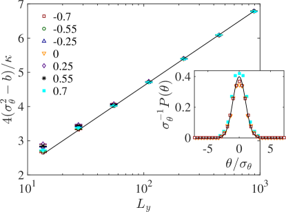
For values near $H=0$ and $H=1$, one has less precision on the results, as the system is strongly influenced by finite-size effects, see e.g. Ref. Schrenk et al. (2013). The results we obtain from the winding angle measurement are, within error bars, in agreement with the previous estimates from the fractal dimension of the accessible perimeter of zero isoheight lines. Indeed, Eq. (5) gives insights into the conformal invariance of the problem Boffetta et al. (2008). Our results in Fig. 1 give some numerical indication that the accessible zero isoheight lines display conformal invariance, which is a prerequisite for $SLE$.

Left-Passage Probability. As we simulate the curves in a bounded rectangular domain, we map conformally the isoheight lines into the upper half-plane, using an inverse Schwarz-Christoffel transformation Posé et al. (2014), to obtain the chordal curve, which splits the system into two sides. For chordal $SLE$ curves, Schramm has computed the probability $P_{\kappa}(\phi)$ that a given point $z=Re^{i\phi}$ in the upper half-plane $\mathbb{H}$ is on the right-hand side of the curve Schramm (2001). This probability only depends on $\phi$ and is given by Schramm’s formula

$$P_{\kappa}(\phi)=\frac{1}{2}+\frac{\Gamma\left(4/\kappa\right)}{\sqrt{\pi}\Gamma\left(\frac{8-\kappa}{2\kappa}\right)}\cot(\phi)_{2}F_{1}\left(\frac{1}{2},\frac{4}{\kappa},\frac{3}{2},-\cot(\phi)^{2}\right),$$ (6)

where $\Gamma$ is the Gamma function and ${}_{2}F_{1}$ is the Gauss hypergeometric function Schrenk and Stevenson . This probability is known as left-passage probability.

We define a set of sample points $S$ in $\mathbb{H}$ for which we measure the left-passage probability in order to compare it to the values predicted by Schramm’s formula (6). To estimate $\kappa$, we minimize the mean square deviation $Q(\kappa)$ between the computed and predicted probabilities,

$$Q\left(\kappa\right)=\frac{1}{|S|}\sum_{z\in S}\left[P(z)-P_{\kappa}(\phi)\right]^{2},$$ (7)

where $\phi=\arg(z)$, $|S|$ is the cardinality of the set $S$, and $P(z)$ the measured left-passage probability at $z$. The estimated value of $\kappa$ corresponds to the point where the minimum of $Q(\kappa)$ is observed.

Figure 2: (color online) Measured rescaled mean square deviation $Q(\kappa)/Q(\kappa_{min})$ as a function of $\kappa/\kappa_{min}$ with $\kappa_{min}$ the value of $\kappa$ where the minimum of $Q(\kappa)$ is attained, for different Hurst exponents $H=-0.7,-0.55,-0.25,0,0.25,0.55,0.7$. We chose $50^{2}$ points in the range $[-0.025L_{x},0.025L_{x}]\times[0.15L_{y},0.25L_{y}]$ with $L_{y}=1024$ and $L_{x}=8L_{y}$, which are then mapped to the upper half-plane through an inverse Schwarz-Christoffel transformation Posé et al. (2014).

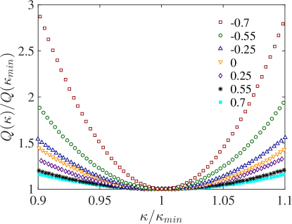
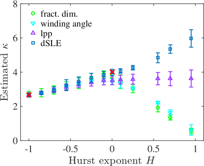
As shown in Fig. 2, for $H<0$, the minimum of $Q$ is less pronounced for higher values of $H$, as it is expected for functions of the form (6) with values of $\kappa$ increasing towards four. As summarized in Table 1, the estimated values of $\kappa$ obtained for negative $H$ are consistent with the ones predicted from $d_{f}$ and confirmed by the winding angle analysis. However, for $H>0$, this is not the case. The obtained $\kappa$ values do not significantly depend on $H$ and are consistently higher than the ones obtained from $d_{f}$. This result suggest that for $H>0$ the curves are not $SLE$.

Direct SLE. To further test if the curves are $SLE$, one has to check that the statistics of the driving function $\xi_{t}$ is consistent with a one-dimensional Brownian motion with variance $\kappa t$. This can be done by solving Eq. (1) numerically. In order to do so, we use the so-called vertical slit map algorithm, where one considers the driving function to be constant over small time intervals $\delta t$. Making this approximation, one can solve Eq. (1) to obtain the following slit map equation Kennedy (2009); Cardy (2005),

$$g_{t}(z)=\xi_{t}+\sqrt{\left(z-\xi_{t}\right)^{2}+4\delta t}.$$ (8)

At $t=0$, one considers the initial curve consisting of the points $\{z_{0}^{0}=0,\ldots,z_{N}^{0}=z_{N}\}$, and sets the driving function to be $\xi_{0}=0$. Then at each iteration $i=1,\ldots,N$, we apply the conformal map $g_{t_{i}}$ to the remaining points $z_{j}^{i-1}$ of the curve, for $j=i,\ldots,N$ to obtain the new mapped curve. One gets a new set of points $z_{j+1}^{i}=g_{t_{i}}(z_{j+1}^{i-1})$ for $j=i,\ldots,N-1$ shorter by one point, by mapping $z_{i}^{i-1}$ to the real axis. For that, in Eq. (8) we set $\xi_{t_{i}}=\mbox{Re}\{z_{i}^{i-1}\}$ and $\delta t_{i}=t_{i}-t_{i-1}=\left(\mbox{Im}\{z_{i}^{i-1}\}\right)^{2}/4$, where $\mbox{Re}\{\}$ and $\mbox{Im}\{\}$ are the real and imaginary parts, respectively.

Figure 3: (color online) Rescaled variance of the driving functions for different values of $H=-0.7,-0.55,-0.25,0,0.25,0.55,0.7$. In the inset, we present the rescaled probability distributions of the driving functions and compare them to a Gaussian distribution for $H=-0.7,0,0.7$.

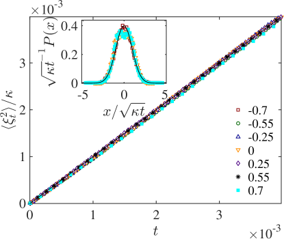
We extracted the driving function of all paths and computed the diffusion coefficient $\kappa$, see values in Table 1, from the variance of the driving function and tested its Gaussian distribution at a fixed Loewner time $t$, see Fig. 3. We find a linear scaling of the variance of the driving function with the Loewner time. However, only for $H\leq 0$, the estimated values of $\kappa$ are consistent with the ones predicted from $d_{f}$. For $H>0$, we obtain values of $\kappa$ significantly higher than the ones expected from $d_{f}$. In fact, the value of $\kappa$ even increases with $H$, instead of decreasing as expected.

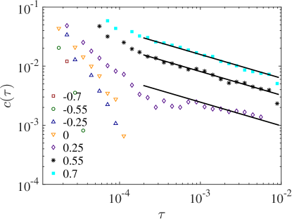
We also test the Markovian property of the driving function by computing the auto-correlation $c(\tau)=\langle c(t,\tau)\rangle_{t}$ of the increments, with

$$c(t,\tau)=\frac{\langle\delta\xi_{t+\tau}\delta\xi_{t}\rangle-\langle\delta\xi_{t+\tau}\rangle\langle\delta\xi_{t}\rangle}{\sqrt{\left(\langle\delta\xi_{t+\tau}^{2}\rangle-\langle\delta\xi_{t+\tau}\rangle^{2}\right)\left(\langle\delta\xi_{t}^{2}\rangle-\langle\delta\xi_{t}\rangle^{2}\right)}},$$ (9)

as shown in Fig. 4, where $\delta\xi_{t}$ is the change in the driving function at time $t$. For $H\leq 0$, the correlation function drops to zero after few time steps, as expected for a Brownian motion. For $H>0$ we observe that the correlation function decays as a power law and thus the driving function is not Markovian, as it shows persistence in the increments. This explains why, though the variance of the driving function is a linear function of time, the statistics of the isoheight lines for $H>0$ are not consistent with $SLE$.

Figure 4: Auto-correlation function $c(\tau)$ of the increments for different values of $H=-0.7,-0.55,-0.25,0,0.25,0.55,0.7$, averaged over $50$ time steps. The solid lines are power laws of exponent $-0.4$.

Conclusion. We numerically showed that the statistics of the accessible perimeter of the zero isoheight lines of long-range correlated landscapes are consistent with $SLE$ only for $-1\leq H\leq 0$. For this range, results for the fractal dimension, winding angle and direct $SLE$ are in agreement within error bars, see Fig. 5. This means that one can describe these curves with a Brownian motion parameterized by a diffusivity $\kappa$. In the two analytic limits $H=-1$ and $H=0$, the accessible perimeters are $SLE_{8/3}$ and $SLE_{4}$ for $H=-1$ and $H=0$, respectively, results that we recover in our numerical analysis. To our knowledge, this is the first time that for an entire range of values of the Hurst exponent $H$, a family of curves coupled to random landscapes is shown to be consistent with $SLE$. This gives new insight in the field of fractional Gaussian Fields in two dimensions Lodhia et al. , what might be helpful for understanding correlated landscapes from a theoretical point of view. One might also wonder if these isoheight lines can be related to some random walk process, as in the case of uncorrelated random landscapes and the Gaussian Free Field. For example, the isoheight lines for $H=-1$ and $H=0$ are two specific cases of the overruled harmonic walker Celani et al. (2009).

Figure 5: (color online) Estimated diffusion coefficients $\kappa$ from the fractal dimension, the winding angle, the left-passage probability (lpp), and the direct $SLE$ methods (dSLE). The red crosses correspond to the rigorous results.

For positive $H$, we show that the driving function also scales linearly in time but it is not Markovian, a necessary condition to establish $SLE$. The numerical data suggest that the auto-correlation function scales as a power law. Credidio et al. showed that if the driving function is a stochastic process with anomalous diffusion, the generated tracers are anisotropic Credidio et al. . In the same spirit, it would be of interest to systematically study the statistics of random curves generated from a driving function with persistence and compare them to isoheight lines.

Table 1: Diffusion coefficient $\kappa$ computed from the fractal dimension $\kappa_{\mathrm{frac}}$ using data from Schrenk et al. (2013) for $H\leq 0$ and obtained numerically for $H>0$ using the yardstick method, from the winding angle $\kappa_{\theta}$, from the left-passage probability $\kappa_{\mathrm{LPP}}$ and the direct $SLE$ method $\kappa_{\mathrm{dSLE}}$, for the different values of the Hurst exponent $H$.

$H$	$\kappa_{\mathrm{frac}}$	$\kappa_{\theta}$	$\kappa_{\mathrm{LPP}}$	$\kappa_{\mathrm{dSLE}}$
$-1$	$2.76\pm 0.16$	$2.66\pm 0.01$	$2.69\pm 0.08$	$2.66\pm 0.12$
$-0.85$	$2.80\pm 0.24$	$2.76\pm 0.02$	$2.80\pm 0.07$	$2.79\pm 0.10$
$-0.7$	$2.96\pm 0.24$	$2.94\pm 0.03$	$2.95\pm 0.11$	$2.97\pm 0.17$
$-0.55$	$3.20\pm 0.24$	$3.14\pm 0.03$	$3.13\pm 0.15$	$3.29\pm 0.32$
$-0.4$	$3.35\pm 0.31$	$3.32\pm 0.03$	$3.27\pm 0.17$	$3.46\pm 0.26$
$-0.25$	$3.64\pm 0.28$	$3.45\pm 0.09$	$3.40\pm 0.21$	$3.67\pm 0.26$
$-0.1$	$3.90\pm 0.18$	$3.49\pm 0.04$	$3.50\pm 0.24$	$3.84\pm 0.20$
$0$	$3.88\pm 0.20$	$3.44\pm 0.18$	$3.52\pm 0.25$	$3.98\pm 0.19$
$0.1$	$3.44\pm 0.40$	$3.44\pm 0.27$	$3.56\pm 0.26$	$4.07\pm 0.13$
$0.25$	$3.04\pm 0.24$	$3.07\pm 0.07$	$3.59\pm 0.29$	$4.26\pm 0.13$
$0.55$	$1.92\pm 0.24$	$2.22\pm 0.08$	$3.62\pm 0.36$	$4.84\pm 0.29$
$0.7$	$1.36\pm 0.16$	$1.65\pm 0.16$	$3.62\pm 0.41$	$5.35\pm 0.25$
$0.95$	$0.56\pm 0.16$	$0.62\pm 0.31$	$3.63\pm 0.50$	$5.97\pm 0.51$

This Letter also opens the possibility of applying $SLE$ to the study of landscapes with negative Hurst exponent $H$. As we have shown, many systems can be considered from the point of view of a landscape, where isoheights are of relevance. Especially, it has been shown that zero vorticity isolines in two-dimensional turbulence are $SLE$ Bernard et al. (2006). There have been also attempts to extend this result to isolines in a generalized Navier-Stokes equation Falkovich and Musacchio to study the conformal invariance of a larger class of turbulence problems. It would be interesting to see if a relation between this problem and our results can be drawn for the accessible perimeters of these contour lines.