Spectral statistics across the many-body localization transition

Abstract

The many-body localization transition (MBLT) between ergodic and many-body localized phase in disordered interacting systems is a subject of much recent interest. Statistics of eigenenergies is known to be a powerful probe of crossovers between ergodic and integrable systems in simpler examples of quantum chaos. We consider the evolution of the spectral statistics across the MBLT, starting with mapping to a Brownian motion process that analytically relates the spectral properties to the statistics of matrix elements. We demonstrate that the flow from Wigner-Dyson to Poisson statistics is a two-stage process. First, fractal enhancement of matrix elements upon approaching the MBLT from the metallic side produces an effective power-law interaction between energy levels, and leads to a plasma model for level statistics. At the second stage, the gas of eigenvalues has local interaction and level statistics belongs to a semi-Poisson universality class. We verify our findings numerically on the XXZ spin chain. We provide a microscopic understanding of the level statistics across the MBLT and discuss implications for the transition that are strong constraints on possible theories.

Introduction. Quantum and statistical mechanics represent two seemingly rather different approaches to the description of complex physical systems. Yet these two viewpoints agree for a wide class of isolated quantum systems, which are said to thermalize Srednicki (1994); Rigol et al. (2008). Determining the circumstances under which an isolated quantum many-body system becomes its own thermal bath and thermalizes itself, just as Baron Munchausen could pull himself out of a mire by his own hair, perhaps using some kind of fluctuation, is an open question.

Phenomena similar to the emergence of thermalization also occur in few-body quantum systems, which frequently show the emergence of so-called quantum chaos Haake (2013). There, upon changing parameters/number of degrees of freedom, the classical system can go from regular to chaotic behavior. On a quantum level this results in changes of level statistics, which has proven to be a powerful probe of the system properties in the context of quantum chaos. In particular, there exist two standard universal limits: Poisson statistics (PS) and Wigner-Dyson level statistics (WDS) Mehta (2014). For few-body systems, PS applies to systems which are classically integrable and do not have any level repulsion. WDS stems from random-matrix theory and holds for generic chaotic systems, where energy levels repel each other (i.e., the energy difference between neighboring levels is statistically unlikely to be small compared to the mean level spacing).

Integrable (non-chaotic) behavior is abundant in the context of few-body physics. On the other hand, in the many-body world the only non-thermalizing phase (in the sense of stability to small perturbations) is represented by many-body localized (MBL) systems Basko et al. (2006); Gornyi et al. (2005). Recent progress established that thermalization fails in the MBL phase due to the existence of extensively many conserved quantities Huse and Oganesyan (2013); Serbyn et al. (2013); Imbrie (2014); Ros et al. (2015). On the other hand, it is known that one can tune the system through a phase transition into a thermalizing ergodic phase Pal and Huse (2010); Bar Lev et al. (2015); Luitz et al. (2015); Vosk et al. (2014); Potter et al. (2015); Goold et al. (2015); De Luca and Scardicchio (2013); Agarwal et al. (2014); Torres-Herrera and Santos (2015); Serbyn et al. (2015). Below we aim to understand the evolution of the level statistics across the MBL-to-ergodic transition, gaining insights into the breakdown of thermalization.

Crossover between PS and WD statistics has been studied extensively in a single-particle physics context: for quantum kicked rotor Izrailev (1989), integrability breaking perturbations Lenz and Haake (1991); Caurier et al. (1990), and single-particle Anderson localization transition (ALT) Shklovskii et al. (1993); Evers and Mirlin (2008); Mirlin (2000). In the many-body problems, PS to WD crossover is also known to occur upon breaking of (quantum) integrability Modak et al. (2014). In most of the examples, the PS and WDS are the only two stable points. The only known exception is the ALT, where universal statistics different from PS and WDS emerges at the mobility edge Shklovskii et al. (1993).

The spectral statistics in the case of MBL transition was demonstrated to evolve from WDS to PS as one localizes the system Oganesyan and Huse (2007); Pal and Huse (2010); Avishai et al. (2002); Modak and Mukerjee (2014), however not much is known about the intermediate statistics. The common probe used to characterize level statistics across MBLT is an average ratio of the consecutive energy spacings Pal and Huse (2010); Luitz et al. (2015); Agarwal et al. (2014); Bar Lev et al. (2015). However, this is a single parameter and it does not provide much insight into the intermediate form of the level statistic, nor into physical details of its crossover.

In this paper we study how the spectral statistics changes across the MBL-delocalization transition. In order to build a microscopic understanding of the level statistics we generalize Dyson’s Brownian motion model Dyson (1962), previously applied to the ALT Chalker et al. (1996), to the many-body case. From the mapping to Brownian motion, we obtain non-trivial relations between fractality De Luca and Scardicchio (2013); Agarwal et al. (2014); Torres-Herrera and Santos (2015); Serbyn et al. (2015), spectral statistics, and properties of matrix elements across the MBLT Nandkishore et al. (2014); Serbyn et al. (2015). While many features can be simultaneously explained in this analysis, one surprise is that there appear to be two different regimes of intermediate spectral statistics: in one, the effective interaction between energy levels in the plasma model has a variable power-law, while in the other, the effective interaction is short-ranged but over a variable number of levels.

Figure 1: (top) Random walk in a space of Hamiltonians induces a stochastic process on the eigenenergies. The interaction between eigenlevels is set by a potential energy $U(s_{i}-s_{j})$. (bottom) Evolution of the interaction between levels $U(s)$ across the MBL transition determines the level statistics.

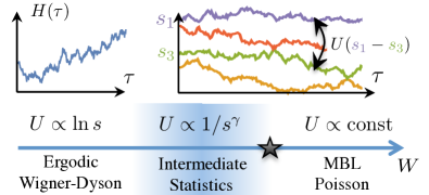
Within the picture of Brownian motion Dyson (1962); Chalker et al. (1996), the level statistics is controlled by the effective interaction between energy levels, see Fig. 1. In particular, deep in the metal phase, the WD statistics emerges from the partition function of a one-dimensional Coulomb gas, where particles interact with a logarithmic potential $U(s)=\log|s|$. At a first stage, upon approaching the MBL transition, the effective interaction starts to decay as a power-law: $U(s_{i}-s_{j})=|s_{i}-s_{j}|^{-\gamma}$ when $|s_{1}-s_{2}|\geq N_{\text{erg}}$. The power-law interaction changes tails of the level statistics, so it can be approximately described by the plasma model, and is intermediate between PS and WDS case. At the second stage, when exponent $\gamma$ becomes bigger than one, the interaction becomes effectively short-ranged, and level spacing distribution tends to the semi-Poisson distribution Bogomolny et al. (1999). In this regime it is the range of the interaction which changes with disorder/system size. As soon as the range of interactions reaches zero, we arrive at Poisson statistics.

Before discussing implications of the above picture of the level statistics, we justify the proposed cartoon using both analytic and numeric arguments. In particular, we argue that the parameter $\gamma$ introduced above can be extracted from the properties of the many-body matrix elements which decay as a power-law with energy separation between eigenstates, where $\gamma\leq 1$ is the same power which controls level statistics. The power-law behavior of matrix elements can be viewed as a generalization of the Chalker-Daniell scaling of wave function overlap Chalker and Daniell (1988) to the many-body case, and it is consistent with fractality of wave functions near MBLT De Luca and Scardicchio (2013); Agarwal et al. (2014); Torres-Herrera and Santos (2015); Serbyn et al. (2015).

Plasma model for level correlations. In the random matrix theory, the joint probability density for random matrix ensembles reads

$$P(\{s_{i}\})=\frac{e^{-\beta H}}{Z},\ H=\sum_{i}W(s_{i})+\sum_{i<j}U(s_{i}-s_{j}),$$ (1)

where $\beta=1$ for orthogonal matrix ensemble which will be of primary interest. The confining potential $W(s)=s^{2}/2$ is parabolic, and interaction is $U(s_{i}-s_{j})=-\ln|s_{i}-s_{j}|$. As Dyson demonstrated in his pioneering work Dyson (1962), this distribution function may be viewed as a stationary distribution of the stochastic random walk in a space of matrices (Hamiltonians).

To derive the joint distribution of eigenenergies from a random walk, one can start from the eigenbasis and perform a stochastic step in the space of Hamiltonians, induced by $\Delta H$. Then, we get the energy correction in a form

$$\Delta s_{n}=V_{nn}+\sum_{m\neq n}\frac{V_{mn}V_{nm}}{s_{n}-s_{m}},\quad V_{mn}=\langle m|\Delta H|n\rangle,$$ (2)

which is the shift of eigenenergies induced by the perturbation $\Delta H$ up to second order. For Gaussian ensembles of random matrices, using $\langle V_{nm}V_{mn}\rangle=\frac{2}{\beta}\Delta\tau$ and $\langle V_{nn}V_{mm}\rangle=\delta_{mn}\Delta\tau$ one can derive Fokker-Planck equation (see Supplemental Material sup for more details). Its stationary (equilibrium) solution is given by Eq. (1) with logarithmic interaction.

Dyson’s mapping was generalized to the case of disordered problems Chalker et al. (1996). For such problems, it is natural to perform a random walk (RW) in a space of Hamiltonians by changing realizations of disorder. As we are going to concentrate on properties of a spin chain in a random magnetic field, which is coupled to the $z$ component of a spin $S^{z}_{i}$, we take $\Delta H=\sum_{i=1}^{L}h_{i}(\tau)S^{z}_{i}$, with $\langle h_{i}(\tau)h_{j}(\tau^{\prime})\rangle=v^{2}\delta(\tau-\tau^{\prime})\delta_{ij}$. Similar to the case of random matrices Dyson (1962); Haake (2013); sup , the two correlators which determine the level dynamics are:

$$\langle V_{nn}V_{mm}\rangle = \delta d_{nm}=\langle n|S^{z}_{i}|n\rangle\langle m|S^{z}_{i}|m\rangle,$$ (3)

$$\langle V_{nm}V_{mn}\rangle = \delta c_{nm}=|\langle m|S^{z}_{i}|n\rangle|^{2},$$ (4)

where we assumed that $v^{2}=\delta/L$, where $\delta$ is the many-body level spacing, so that $s_{n}$ represent unfolded energy spectrum. The correlator (3) sets the spectrum of a random noise, while spectral function $c_{nm}$ determines the interaction between levels in the ensemble.

Effective interaction between levels. The RW process depends crucially on two correlators Eqs. (3)-(4). To make analytic progress we use a mean-field like approximation Chalker et al. (1996), assuming that $d_{nm}$ and $c_{nm}$ can be replaced by their ensemble averages,

$$c(\omega)=\langle c_{nm}\delta(s_{n}-s_{m}-\omega)\rangle,$$ (5)

(and similar expression for $d_{nm}$) which now depend only on the energy difference between eigenstates. For the single-particle Anderson localization, the $c_{nm}$ and $d_{nm}$ necessarily coincide with the wave functions overlaps Chalker et al. (1996), $c_{nm}=d_{nm}\propto\int dx|\psi_{n}(\tau,x)|^{2}|\psi_{m}(\tau,x)|^{2}$. The fractality of the wave function near the mobility edge results in a power-law enhancement of $c(\omega)\propto A/\omega^{\gamma}$ Chalker and Daniell (1988); Cuevas and Kravtsov (2007). In the case of ALT this enhancement arises because the envelope of wave functions nearby in energy lives on the same multifractal domain Cuevas and Kravtsov (2007). In the many-body case similar enhancement can arise from the fractal structure of the wave function in the Hilbert space in a vicinity of MBLT De Luca and Scardicchio (2013); Agarwal et al. (2014); Torres-Herrera and Santos (2015); Serbyn et al. (2015).

Inspired by the approach recently proposed in Ref. Serbyn et al. (2015), we apply the fractal scaling to the matrix elements of a local operators. In particular, we assume that the inverse participation ratio (IPR), $I_{2}={\cal V}\sum_{j}|V_{ij}|^{4}\propto{\cal V}^{-d_{2}}$, where $d_{2}$ is generalized fractal dimension, and ${\cal V}=\exp(sL)$ is the number of states in the Hilbert space. Using scaling, we translate the IPR into the scaling with the distance in the Hilbert space as ${\cal V}^{2}\langle V_{ii}^{2}V_{ik}^{2}\rangle\propto({\cal V}/{\cal R})^{1-d_{2}}$, where ${\cal R}=\exp(sd_{i,k})$ grows exponentially with (humming) distance in the Hilbert space, $d_{i,k}$. From here, expressing $\cal V$ via frequency, as $\delta_{\cal V}=J/{\cal{V}}=\omega$, we get: ${\cal V}^{2}\langle V_{ii}^{2}V_{ki}^{2}\delta(E_{i}-E_{k}-\omega)\rangle\propto(J/\omega)^{1-d_{2}}$. Finally, omitting the diagonal matrix element, we arrive to the scaling:

$$c(\omega)\propto\left(\frac{J}{\omega}\right)^{\gamma},\qquad\gamma=1-d_{2}.$$ (6)

Note, that we did not discuss the microscopic nature of a fractal behavior, although Griffiths (rare-region) effects Agarwal et al. (2014) in vicinity of MBL transition is one possible microscopic scenario. Also, relating $d_{2}$ to the properties of matrix elements, i.e. exponent $\kappa$ in the scaling Nandkishore et al. (2014); Serbyn et al. (2015), $|V_{nm}|\propto\exp(-(s+\kappa)L)$ is an interesting question.

The correlation between diagonal matrix elements, the function $d_{nm}$ also shows a power-law dependence. However, there is an enhancement of $d_{nm}$ for $n=m$, allowing to approximate $d(\omega)$ as a delta-function, see SM for additional discussion sup .

Implications for spectral statistics. Using power-law form of $c(\omega)$ Eq. (6), and the delta-function form of $d(\omega)$ we can map our model onto the plasma model for the level statistics Kravtsov and Lerner (1995), provided $\gamma<1$. The plasma model assumes a power-law interaction potential $U(s)=A/|s|^{\gamma}$ in the joint distribution function (1). It predicts the tails of the level statistics $P(s)\propto s^{\beta}\exp(-h_{\gamma}s^{2-\gamma})$ for $s\gg 1$, and variance of the number of levels in a box of size $N$ becomes $\mathop{\rm var}N\propto N^{\gamma}$, which is intermediate between WD-like rigidity $\mathop{\rm var}N\propto\log N$ and Poisson case Haake (2013); Mehta (2014).

For larger values of $\gamma\geq 1$ the effective interaction in the gas of eigenvalues becomes short range, and mapping to the plasma model no longer works. Instead, spectral properties now are expected to be well-described by a family of semi-Poisson distributions Bogomolny et al. (1999), which arise from a gas of eigenvalues with a finite-range interaction. They predict Poisson-like behavior of the tails of $P(s)$ and level compressibility $P(s)\propto s^{\beta}e^{-(\beta h+1)s}$, and $\mathop{\rm var}N\propto\chi N$ with $\chi\leq 1$, where $h$ is the range of interactions. Such level statistics has been dubbed “critical” in the literature Kravtsov and Muttalib (1997); Muttalib et al. (1993); García-García and Verbaarschot (2003) and is believed to describe the level statistics at the ALT Evers and Mirlin (2008); Mirlin (2000).

Figure 2: Averaged function $c(E)$ evolves from being almost flat at low disorder ($W=0.5$) to a power-law decay. Note that for the intermediate values of disorder, matrix element is enhanced at small energy difference compared to the limit of weak disorder.

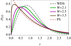
Using the above intuition, we propose the following form of the level spacing distribution and spectral rigidity to interpolate between WDS and PS,

$$P(s;\beta,\gamma_{P})=C_{1}x^{\beta}\exp\left(-C_{2}x^{2-\gamma_{P}}\right),\ \mathop{\rm var}N=\chi N^{\gamma_{\rm var}},$$ (7)

where the parameter $1\geq\gamma_{P},\gamma_{\rm var}\geq 0$ controls the tails of the statistics and level rigidity, and $1\geq\beta\geq 0$ determines the level repulsion. The constants $C_{1,2}$ can be fixed by requiring that $\langle 1\rangle=\langle s\rangle=1$. When $\gamma_{P}=0$, this distribution becomes WD. In the opposite limit, $\gamma_{P}\to 1$, distribution (7) becomes a semi-Poission with generic $\beta$. For the spectral rigidity our interpolating function also can describe the (semi-)Poisson limit, however failing to capture logarithmic growth of $\mathop{\rm var}N$ in the WD case.

Figure 3: (a) Evolution of level spacing distributions as system is tuned towards MBL phase. Points represent data, while solid lines are best fits with a two-parameter distribution (7). Red and black dashed lines correspond to Poisson and Wigner-Dyson distribution. (b) The exponent $\gamma_{P}$, controlling tails of level statistics, flows with $L$ for $W\lesssim 2.5$, but is constant in vicinity of MBLT $W_{c}\approx 3.6$. (c) In contrast, $\beta$ controlling the level repulsion, remains constant for $W\lesssim 2$, and starts to flow closer to the MBLT.

Numerical results. We use the XXZ spin chain in a random field as a specific model with a previously located MBL transition Pal and Huse (2010) to test our picture of level statistics. The Hamiltonian is

$$\hat{H}_{\text{XXZ}}=\sum_{\langle ij\rangle}{{\bf S}}_{i}\cdot{{\bf S}}_{j}+\sum_{i}w_{i}S_{i}^{z},\quad S^{x,y,z}=\frac{1}{2}{\bf\sigma}^{x,y,z},$$ (8)

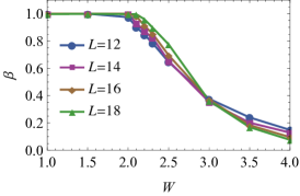
where disorder enters via random fields $w_{i}$ uniformly distributed in the interval $[-W;W]$. We perform exact diagonalization for chains of size $L=12,\ldots 16(18)$ with periodic boundary conditions to extract properties of matrix elements (spectral statistics). We use central part of the many-body spectrum, which corresponds to energy density $\varepsilon=(E-E_{\text{min}})/(E_{\text{max}}-E_{\text{min}})=0.45\pm 0.1$. The MBL transition at this energy density is believed to occur near $W_{c}\approx 3.6$ Luitz et al. (2015). To unfold levels, we fit the staircase function with a 3rd order polynomial. We use both local and global level unfolding schemes Gómez et al. (2002).

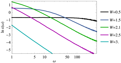
We start by discussing the numerical results for averaged $c(\omega)$, presented in Fig. 2(a). Upon increasing disorder, we see the crossover of $c(\omega)$ from a constant to a power-law decay. As one may expect, this crossover happens at some scale, $N_{\text{erg}}$, so that $c(\omega<N_{\text{erg}})\propto\text{const}$, and decays as a power-law beyond $\omega>N_{\text{erg}}$. The additional scale $N_{\text{erg}}$ has a meaning similar to the correlation length, over which ergodicity holds. As $N_{\text{erg}}\to 0$, interaction between levels becomes critical even for the smallest separations.

From the power-law form of $c(\omega)$, we expect that level spacing distribution for the XXZ spin chain to be well described by Eq. (7). Fig. 3(a) illustrates that the flow of the level statistics is indeed well captured by Eq. (7). The $P(s)$ for disorder $W<2$ is not shown, as it looks very similar to WD distribution: since $P(s)$ is influenced the most by the interaction between close levels, $N_{\text{erg}}$ must become close to zero before we see the flow in the level statistics. In contrast to the level statistics, which is influenced by a non-critical part of $c(\omega)$, the spectral rigidity is expected to be less sensitive to the behavior of $c(\omega)$ at small $\omega$. In SM sup we show that $\mathop{\rm var}N$ behaves as a power-law (7), and becomes linear for $W\gtrsim 2$. Also, we test that different estimates for exponent $\gamma$ show reasonable agreement as follows from plasma model.

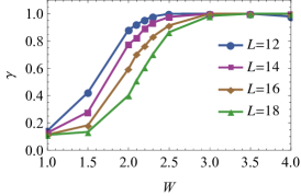
Finally, we consider the flow of parameters $\gamma_{P}$ and $\beta$ with increasing system size, presented in Fig. 3(b)-(c). While $\gamma_{P}$ controlling tails of the level statistics has a strong flow at disorder $W\leq 2.5$, at larger disorders $\gamma_{P}$ is very close to one and changes little with $L$. This further supports the conclusion that for $W\geq 2.5$ the effective interaction between energy levels becomes short-ranged for the largest accessible system sizes. Consistent with our expectation, $\beta$ shown in Fig. 3(c) changes weakly when statistics is described by plasma model ($W\leq 2$), and begins to flow once level interactions are local.

Discussion and open questions. Using analytical and numerical arguments we described the spectral properties across MBL transition using a two-stage flow picture. Note that we need at least two parameters, $\gamma$ and $N_{\text{erg}}$, to describe level statistics. This is not surprising if we recall that even the case of ALT, the existence of multifractality means that to describe the universal properties one requires more information beyond the small number of critical indices needed for a simple thermodynamic phase transition Evers and Mirlin (2008); Mirlin (2000). Below we discuss the implications of the proposed picture of the spectral statistics flow.

At the first stage the “correlation length” $N_{\text{erg}}$ shrinks to zero, but the exponent responsible for level interactions $\gamma$ is smaller than one. Intuitively, the levels beyond correlation length become more and more different, corresponding to a gradual breakdown of the ETH. Here the level statistics can be described by the effective plasma model. Although this model was proposed some time ago Kravtsov and Lerner (1995), it does not apply in the case of ALT, despite the presence of multifractality near single particle mobility edge. Hence, to the best of our knowledge, the present study is the first physical realization of the plasma model.

The second stage begins at $W\geq 2.5$, when $\gamma\geq 1$ so that interactions between levels are local. Although we cannot exclude the finite size effects, the numerical estimates for the MBL transition at $W_{c}\approx 3.6$ suggest that at the MBL transition interactions between levels are local. Thus, we conjecture that level statistics near and at the MBLT belongs to the same or similar “critical” family as the universal statistics at the ALT Kravtsov and Muttalib (1997); Muttalib et al. (1993); García-García and Verbaarschot (2003). This also naturally explains why the average ratio of the level spacing $r=\min(\delta_{n},\delta_{n+1})/\max(\delta_{n},\delta_{n+1})$ at the MBLT, widely used in the literature Pal and Huse (2010); Luitz et al. (2015); Agarwal et al. (2014); Bar Lev et al. (2015), is very close to the value expected from PS.

The semi-Poisson level statistics emerges at the same value of disorder where the boundary of the Griffiths phase was previously identified in the literature Agarwal et al. (2014), $W\approx 2.5$ (Refs. De Luca and Scardicchio (2013); Goold et al. (2015) report the onset of ergodicity breaking at the same location). The existing theories of the MBLT Vosk et al. (2014); Potter et al. (2015) predict extensive entanglement and subdiffusive transport in the ergodic phase. The wide region of critical statistics near transition may be a manifestation of finite size effects (system sizes studied are smaller that diverging correlation length). Indeed the strong overlaps only between adjacent energy levels imply logarithmic transport Serbyn et al. (2015), predicted at the MBLT Vosk et al. (2014); Potter et al. (2015). On the other hand, existence of thermodynamically stable Griffiths phase is another intriguing possibility.

In closing, we have found that Dyson’s mapping of level statistics to Brownian motion allows one to understand the spectral statistics in the MBL transition at least as well as in the ALT for which it was introduced. There are basic differences between the two transitions, e.g., several quantities which are uniquely defined at the ALT allow inequivalent generalizations to the MBLT. There are two steps of the spectral statistics flow, one with long-range interactions (the plasma model) and one with local interactions, and the boundary between the two is found numerically to coincide with the onset of a Griffiths phase and subdiffusive transport. Since level statistics are known to be the simplest universal probe of the transition to quantum chaos in simpler problems, understanding the origin and universality of the two-step plasma model of level statistics is an important challenge for theories of the MBLT.

Acknowledgements. M.S. acknowledges useful discussions with V. Kravtsov, D. Abanin, Z. Papic, E. Mucciolo, A.C. Potter, R. Vasseur, and S. Gazit. M.S. was supported by Gordon and Betty Moore Foundation’s EPiQS Initiative through Grant GBMF4307. J.E.M. was supported by NSF DMR-1206515 and the Simons Foundation.

Supplemental Online Material for “Spectral statistics across the many-body localization transition”

Below we present additional details on the derivation of the level statistics from the Brownian motion. In particular, we discuss the approximation for $d(\omega)$ used in the main text. In the second part we discuss the behavior of the spectral rigidity, and compare various estimates for exponent $\gamma$.

.1 Analytic derivation of level statistics from the Brownian motion

.1.1 Wigner-Dyson statistics

Let us begin with reproducing the WD statistics from the Brownian motion model. We assume the Brownian motion in the space of random matrices,

$$H(\tau)=H_{0}+\int_{0}^{\tau}d\tau\,V(\tau),$$ (S1)

where matrix $V(\tau)$ satisfies the following properties:

$$\langle V_{nm}(\tau)\rangle = -H_{nm}(\tau),$$ (S2)

$$\langle V_{nm}(\tau)V_{mn}(\tau^{\prime})\rangle = \delta(\tau-\tau^{\prime}),$$ (S3)

$$\langle V_{nn}(\tau)V_{mm}(\tau^{\prime})\rangle = \frac{2}{\beta_{RM}}\delta(\tau-\tau^{\prime})\delta_{nm}.$$ (S4)

Parameter $\beta_{RM}$ specifies the symmetry class, $\beta_{RM}=1$ for GOE, and $\beta_{RM}=2$ for GUE.

For convenience, we fix the basis to coincide with the (instantaneous) eigenbasis of $H(\tau)$. We apply the perturbation theory to calculate correction to eigenvalues of $H(\tau)$, $\{s_{n}\}$ induced by the change in the matrix

$$\Delta V=\int_{\tau}^{\tau+\Delta\tau}d\tau\,V(\tau).$$ (S5)

Resulting correction to $s_{n}$ reads:

$$\Delta s_{n}=\Delta V_{nn}+\sum_{m\neq n}\frac{|\Delta V_{nm}|^{2}}{s_{n}-s_{m}}.$$ (S6)

Averaging this equation over $V$ using the fact that $H_{nn}=s_{n}$ in the eigenbasis, we get:

$$\langle\Delta s_{n}\rangle = \mu_{n}(\{s\})\Delta\tau,$$ (S7)

$$\mu_{n}[\{s\}] = -s_{n}+\sum_{m\neq n}\frac{1}{s_{n}-s_{m}}.$$ (S8)

Using the second moment

$$\langle\Delta s_{n}\Delta s_{m}\rangle=\frac{2}{\beta_{RM}}\delta_{nm}\Delta\tau,$$ (S9)

we find that $s_{n}(\tau)$ obeys the following Langevin equation:

$$\frac{ds_{n}}{d\tau}=\mu_{n}[\{s\}]+\xi_{n}(\tau),$$ (S10)

where drift term is given by Eq. (S8) and white noise is specified by

$$\langle\xi_{n}(\tau)\xi_{m}(\tau^{\prime})\rangle = \frac{2}{\beta_{RM}}\delta_{nm}\delta(\tau-\tau^{\prime}).$$ (S11)

Translating the Langevin equation into the Fokker-Planck equation governing the evolution of the joint probability distribution function $P(\{s_{n}\},\tau)$, we get:

$$\frac{\partial P(\{s\},\tau)}{\partial\tau}=\sum_{n}\left\{-\frac{\partial}{\partial s_{n}}[\mu_{n}(\{s\})P(\{s\},\tau)]\right.\\ \left.+\frac{1}{\beta_{RM}}\frac{\partial^{2}}{\partial s_{n}^{2}}P(\{s\},\tau)]\right\}.$$ (S12)

Using explicit expression for the drift, Eq. (S8) we see that the joint probability distribution

$$P(\{s\})=C\prod_{m<n}|s_{n}-s_{m}|^{\beta_{RM}}\exp\left(-\frac{\beta_{RM}}{2}\sum_{n}s_{n}^{2}\right)$$ (S13)

is a stationary solution of the Fokker-Planck equation (S12). This distribution function corresponds to Wigner-Dyson statistics. It is equivalent to the partition function of plasma with logarithmic repulsion and a parabolic confining potential.

Figure S1: Normalized diagonal correlator $\langle d_{nm}\rangle/\langle d_{nn}\rangle$ as a function of $|m-n|$ for different values of disorder. Although for intermediate disorders $\langle d_{nm}\rangle$ decays as a power-law with $|n-m|$, the value of $d_{nn}$ is significantly enhanced, compared to the power-law tail.

.1.2 Plasma model

After discussing the random matrix example, we move on to the many-body case. There the Brownian motion is induced by a random walk over different realizations of disorder. For a specific case of XXZ spin chain in a random magnetic field, we have

$$V(\tau)=\sum_{i=1}^{L}h_{i}(\tau)S^{z}_{i},\quad\langle h_{i}(\tau)h_{j}(\tau)\rangle=v^{2}\delta(\tau-\tau^{\prime})\delta_{ij}.$$ (S14)

Repeating the procedure outlined above for the case of random matrices, we get the following Langevin equation:

$$\frac{ds_{n}}{d\tau}=\mu_{n}[\{s\},\tau]+\xi_{n}(\tau),$$ (S15)

with drift and noise terms reading:

$$\mu_{n}[\{s\},\tau] = \frac{v^{2}}{\delta}\sum_{i=1}^{L}\sum_{m\neq n}\frac{c^{i}_{nm}(\tau)}{s_{n}-s_{m}},$$ (S16)

$$\langle\xi_{n}(\tau)\xi_{m}(\tau^{\prime})\rangle = \frac{v^{2}}{\delta}\sum_{i=1}^{L}d^{i}_{nm}(\tau)\delta(\tau-\tau^{\prime}),$$ (S17)

where the level spacing $\delta$ appeared since we assume that $s$ represents unfolded energy spectrum with mean level spacing of one. The correlation functions $c_{nm}$ and $d_{nm}$ are defined by the matrix elements of the operator $S^{z}_{i}$ on a site $i$ (which couples to the random magnetic field) in the instantaneous eigenbasis:

$$c^{i}_{nm}(\tau) = \frac{1}{\delta}\langle n|S^{z}_{i}|m\rangle\langle m|S^{z}_{i}|n\rangle,$$ (S18)

$$d^{i}_{nm}(\tau) = \frac{1}{\delta}\langle n|S^{z}_{i}|n\rangle\langle m|S^{z}_{i}|m\rangle.$$ (S19)

The mean field approximation employed in the main text amounts to replacing $c^{i}_{nm}(\tau)$ and $d^{i}_{nm}(\tau)$ with their average over ensemble, which becomes only a function of $n-m$. Fixing $v^{2}=\delta/L$ to cancel the level spacing from resulting equations, we get the following Lagnevin dynamics:

$$\frac{ds_{n}}{d\tau}=\mu_{n}[\{s\},\tau]+\xi_{n}(\tau),$$ (S20)

with drift and noise terms

$$\mu_{n}[\{s\},\tau] = \sum_{m\neq n}\frac{c(s_{n}-s_{m})}{s_{n}-s_{m}},$$ (S21)

$$\langle\xi_{n}(\tau)\xi_{m}(\tau^{\prime})\rangle = d(s_{n}-s_{m})\delta(\tau-\tau^{\prime}),$$ (S22)

expressed via rescaled correlators:

Assuming a delta-function form of $d(\omega)$, and a power-law ansatz for $c(\omega)$,

$$c(\omega)=\frac{A}{|\omega|^{\gamma}},\quad 0<\gamma<1,$$ (S23)

the stationary solution of corresponding Fokker-Planck equation reproduces the partition function of plasma with interaction potential given by:

$$U(s)=\frac{C}{|s|^{\gamma}}.$$ (S24)

.1.3 Numerical results for $d(\omega)$

In order to check the validity of approximating $d(\omega)$ by a delta-function, we calculate $d_{nm}$ numerically for the XXZ spin chain. Figure S1 reveals the evolution of average $\langle d_{nm}\rangle$ for different system sizes and disorders. At disorder $W=0.5$, when system is in the ergodic phase, we see that $d_{nm}$ when $|m-n|>0$ does not depend on $|m-n|$, which is a manifestation of the eigenstate thermalization hypothesis(ETH). Nevertheless, values of $\langle d_{nm}\rangle$ for $n\neq m$ are suppressed compared to $d_{nn}$. Even nearby eigenstates can have average spin of different sign, this does not contradict to the ETH which rigorously applies to coarse-grained observables.

For larger disorder, $W>1.5$, the $d_{nm}$ decays approximately as power-law. Nevertheless, the value of $d_{nn}$ is still considerably enhanced, hence a proper approximation for the $d(\omega)$ is $d(\omega)=c_{1}\delta(\omega)+c_{2}/\omega^{\gamma^{\prime}}$ [scaling of the relative weight of delta function in $d(\omega)$ in the thermodynamic limit is an interesting and open question]. Presence of the delta-function contribution in $d(\omega)$ is sufficient to make the spectral statistics different compared to the case of Anderson transition. In particular, repeating the mean-field treatment of Ref. Chalker et al. (1996), we do not get constant spectral form-factor $K(t,\tau)$ in the limit $t\to 0$. This suggests that level compressibility is vanishing, consistent with plasma model Kravtsov and Lerner (1995).

.2 Spectral rigidity and different estimates for $\gamma$ across the MBL transition

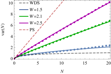
To probe the spectral rigidity, we study the behavior of the variance of number of levels in the box of size $N$. The variance $\mathop{\mathrm{var}}N$ as a function of the box size is shown in Fig. S2 for $L=16$ spins, along with the power-law fits of its behavior. The exponent extracted from the fits, $\gamma_{\text{var}}$ below is compared to exponents extracted by other means.

Figure S2: Variance of the level number in the box of size $N$ becomes essentially linear in $N$ for disorder above $W\geq 2.5$. To minimize the influence of the unfolding procedure, we show and use the part where results agree for both local and global unfolding. All data is for $L=16$ spins.

Figure S3: Exponent $\gamma$ extracted from $c(\omega)$ agrees reasonably with the exponent $\gamma_{\text{var}}$ from the tails of the level statistic. The exponent $\gamma_{P}$ governing the tails of the $P(s)$ is consistently smaller, but agrees with $\gamma^{\prime}=(d\ln c(\omega)/d\ln\omega)_{\omega=0}$.

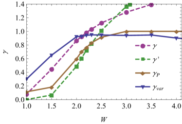
Three exponents, $\gamma,\gamma_{P},\gamma_{\text{var}}$, obtained from matrix elements, level statistics, and level rigidity respectively, are expected to coincide in the region of applicability of plasma model. In Fig. S3 we plot these exponents as a function of disorder for spin chains with $L=16$ spins. We observe the reasonable agreement between the values of $\gamma_{\text{var}}$ and $\gamma$ measured from the tails of level statistics. On the other hand, $\gamma_{P}$ is consistently smaller, and matches much better the $\gamma^{\prime}$, logarithmic derivative of $c(\omega)$ at $\omega\to 0$, confirming that $P(s)$ is more strongly influenced by a non-universal part in the $c(\omega)$. Both $\gamma$ and $\gamma^{\prime}$ become larger than one at $W\approx 2.5$, indicating that for larger disorders the level statistics enters a semi-Poisson regime.

References

- Srednicki (1994) M. Srednicki, Chaos and quantum thermalization, Phys. Rev. E 50, 888 (1994).
- Rigol et al. (2008) M. Rigol, V. Dunjko, and M. Olshanii, Thermalization and its mechanism for generic isolated quantum systems, Nature 452, 854 (2008).
- Haake (2013) F. Haake, Quantum Signatures of Chaos, Springer Series in Synergetics (Springer Berlin Heidelberg, 2013).
- Mehta (2014) M. Mehta, Random Matrices: Revised and Enlarged Second Edition, Pure and Applied Mathematics (Elsevier Science, 2014).
- Basko et al. (2006) D. Basko, I. Aleiner, and B. Altshuler, Metal–insulator transition in a weakly interacting many-electron system with localized single-particle states, Annals of Physics 321, 1126 (2006).
- Gornyi et al. (2005) I. V. Gornyi, A. D. Mirlin, and D. G. Polyakov, Interacting electrons in disordered wires: Anderson localization and low- transport, Phys. Rev. Lett. 95, 206603 (2005).
- Huse and Oganesyan (2013) D. A. Huse and V. Oganesyan, A phenomenology of certain many-body localized systems, ArXiv e-prints (2013), arXiv:1305.4915 .
- Serbyn et al. (2013) M. Serbyn, Z. Papić, and D. A. Abanin, Local conservation laws and the structure of the many-body localized states, Phys. Rev. Lett. 111, 127201 (2013).
- Imbrie (2014) J. Z. Imbrie, Arxiv e-prints (2014), 1403.7837 .
- Ros et al. (2015) V. Ros, M. Müller, and A. Scardicchio, Integrals of motion in the many-body localized phase, Nuclear Physics B 891, 420 (2015).
- Pal and Huse (2010) A. Pal and D. A. Huse, Many-body localization phase transition, Phys. Rev. B 82, 174411 (2010).
- Bar Lev et al. (2015) Y. Bar Lev, G. Cohen, and D. R. Reichman, Absence of diffusion in an interacting system of spinless fermions on a one-dimensional disordered lattice, Phys. Rev. Lett. 114, 100601 (2015).
- Luitz et al. (2015) D. J. Luitz, N. Laflorencie, and F. Alet, Many-body localization edge in the random-field heisenberg chain, Phys. Rev. B 91, 081103 (2015).
- Vosk et al. (2014) R. Vosk, D. A. Huse, and E. Altman, Theory of the many-body localization transition in one dimensional systems, ArXiv e-prints (2014), arXiv:1412.3117 [cond-mat.dis-nn] .
- Potter et al. (2015) A. C. Potter, R. Vasseur, and S. A. Parameswaran, Universal properties of many-body delocalization transitions, ArXiv e-prints (2015), arXiv:1501.03501 [cond-mat.dis-nn] .
- Goold et al. (2015) J. Goold, S. R. Clark, C. Gogolin, J. Eisert, A. Scardicchio, and A. Silva, Total correlations of the diagonal ensemble herald the many-body localization transition, ArXiv e-prints (2015), arXiv:1504.06872 [cond-mat.dis-nn] .
- De Luca and Scardicchio (2013) A. De Luca and A. Scardicchio, Ergodicity breaking in a model showing many-body localization, Europhys. Lett. 101, 37003 (2013).
- Agarwal et al. (2014) K. Agarwal, S. Gopalakrishnan, M. Knap, M. Mueller, and E. Demler, Anomalous diffusion and Griffiths effects near the many-body localization transition, ArXiv e-prints (2014), arXiv:1408.3413 [cond-mat.dis-nn] .
- Torres-Herrera and Santos (2015) E. J. Torres-Herrera and L. F. Santos, Dynamics at the Many-Body Localization Transition, ArXiv e-prints (2015), arXiv:1501.05662 [cond-mat.dis-nn] .
- Serbyn et al. (2015) M. Serbyn, Z. Papic, and D. A. Abanin, A criterion for many-body localization-delocalization phase transition, ArXiv e-prints (2015), arXiv:1507.01635 [cond-mat.dis-nn] .
- Izrailev (1989) F. M. Izrailev, Intermediate statistics of the quasi-energy spectrum and quantum localisation of classical chaos, Journal of Physics A: Mathematical and General 22, 865 (1989).
- Lenz and Haake (1991) G. Lenz and F. Haake, Reliability of small matrices for large spectra with nonuniversal fluctuations, Phys. Rev. Lett. 67, 1 (1991).
- Caurier et al. (1990) E. Caurier, B. Grammaticos, and A. Ramani, Level repulsion near integrability: a random matrix analogy, Journal of Physics A: Mathematical and General 23, 4903 (1990).
- Shklovskii et al. (1993) B. I. Shklovskii, B. Shapiro, B. R. Sears, P. Lambrianides, and H. B. Shore, Statistics of spectra of disordered systems near the metal-insulator transition, Phys. Rev. B 47, 11487 (1993).
- Evers and Mirlin (2008) F. Evers and A. D. Mirlin, Anderson transitions, Rev. Mod. Phys. 80, 1355 (2008).
- Mirlin (2000) A. D. Mirlin, Statistics of energy levels and eigenfunctions in disordered systems, Physics Reports 326, 259 (2000).
- Modak et al. (2014) R. Modak, S. Mukerjee, and S. Ramaswamy, Universal power law in crossover from integrability to quantum chaos, Phys. Rev. B 90, 075152 (2014).
- Oganesyan and Huse (2007) V. Oganesyan and D. A. Huse, Localization of interacting fermions at high temperature, Phys. Rev. B 75, 155111 (2007).
- Avishai et al. (2002) Y. Avishai, J. Richert, and R. Berkovits, Level statistics in a heisenberg chain with random magnetic field, Phys. Rev. B 66, 052416 (2002).
- Modak and Mukerjee (2014) R. Modak and S. Mukerjee, Finite size scaling in crossover among different random matrix ensembles in microscopic lattice models, New Journal of Physics 16, 093016 (2014).
- Dyson (1962) F. J. Dyson, A Brownian-Motion Model for the Eigenvalues of a Random Matrix, Journal of Mathematical Physics 3, 1191 (1962).
- Chalker et al. (1996) J. T. Chalker, I. V. Lerner, and R. A. Smith, Random walks through the ensemble: Linking spectral statistics with wave-function correlations in disordered metals, Phys. Rev. Lett. 77, 554 (1996).
- Nandkishore et al. (2014) R. Nandkishore, S. Gopalakrishnan, and D. A. Huse, Spectral features of a many-body-localized system weakly coupled to a bath, Phys. Rev. B 90, 064203 (2014).
- Bogomolny et al. (1999) E. B. Bogomolny, U. Gerland, and C. Schmit, Models of intermediate spectral statistics, Phys. Rev. E 59, R1315 (1999).
- Chalker and Daniell (1988) J. T. Chalker and G. J. Daniell, Scaling, diffusion, and the integer quantized hall effect, Phys. Rev. Lett. 61, 593 (1988).
- (36) See Supplemental Material.
- Cuevas and Kravtsov (2007) E. Cuevas and V. E. Kravtsov, Two-eigenfunction correlation in a multifractal metal and insulator, Phys. Rev. B 76, 235119 (2007).
- Kravtsov and Lerner (1995) V. E. Kravtsov and I. V. Lerner, Effective plasma model for the level correlations at the mobility edge, Journal of Physics A: Mathematical and General 28, 3623 (1995).
- Kravtsov and Muttalib (1997) V. E. Kravtsov and K. A. Muttalib, New class of random matrix ensembles with multifractal eigenvectors, Phys. Rev. Lett. 79, 1913 (1997).
- Muttalib et al. (1993) K. A. Muttalib, Y. Chen, M. E. H. Ismail, and V. N. Nicopoulos, New family of unitary random matrices, Phys. Rev. Lett. 71, 471 (1993).
- García-García and Verbaarschot (2003) A. M. García-García and J. J. M. Verbaarschot, Critical statistics in quantum chaos and calogero-sutherland model at finite temperature, Phys. Rev. E 67, 046104 (2003).
- Gómez et al. (2002) J. M. G. Gómez, R. A. Molina, A. Relaño, and J. Retamosa, Misleading signatures of quantum chaos, Phys. Rev. E 66, 036209 (2002).