Frequency-domain gravitational waves from non-precessing black-hole binaries.
II. A phenomenological model for the advanced detector era

Abstract

We present a new frequency-domain phenomenological model of the gravitational-wave signal from the inspiral, merger and ringdown of non-precessing (aligned-spin) black-hole binaries. The model is calibrated to 19 hybrid effective-one-body–numerical-relativity waveforms up to mass ratios of 1:18 and black-hole spins of $|a/m|\sim 0.85$ ($0.98$ for equal-mass systems). The inspiral part of the model consists of an extension of frequency-domain post-Newtonian expressions, using higher-order terms fit to the hybrids. The merger-ringdown is based on a phenomenological ansatz that has been significantly improved over previous models. The model exhibits mismatches of typically less than 1% against all 19 calibration hybrids, and an additional 29 verification hybrids, which provide strong evidence that, over the calibration region, the model is sufficiently accurate for all relevant gravitational-wave astronomy applications with the Advanced LIGO and Virgo detectors. Beyond the calibration region the model produces physically reasonable results, although we recommend caution in assuming that any merger-ringdown waveform model is accurate outside its calibration region. As an example, we note that an alternative non-precessing model, SEOBNRv2 (calibrated up to spins of only 0.5 for unequal-mass systems), exhibits mismatch errors of up to 10% for high spins outside its calibration region. We conclude that waveform models would benefit most from a larger number of numerical-relativity simulations of high-aligned-spin unequal-mass binaries.

I Introduction

The first direct gravitational wave (GW) detection is anticipated sometime during the operation of the Advanced Laser Interferometer Gravitational-wave Observatory (aLIGO) Abbott et al. (2009); Harry and LIGO Scientific Collaboration (2010); Shoemaker and the Advanced LIGO Team (2009) and Advanced Virgo (AdV) Accadia et al. (2011) detectors Aasi et al. (2013a), beginning with aLIGO in 2015. One of the most likely sources for the first detections, and a rich source of scientific information about both fundamental physics and astrophysics Sathyaprakash and Schutz (2009) are the inspiral and merger of binary black hole (BBH) systems. Observations and measurements of BBH will rely on accurate theoretical models of their GW signal, and the construction of such models is currently an active research topic Hannam (2014).

To date most effort has focussed on binaries where the spin of each black hole (BH) is either zero, or aligned with the binary’s orbital angular momentum. In these configurations the orbital plane and spin directions remain fixed, and the resulting GW signal is far simpler than in generic (precessing) configurations. Recent work has suggested that aligned-spin models may allow detection of most (even precessing) binaries Ajith et al. (2011); Harry et al. (2014); Dal Canton et al. (2015), and also that accurate approximate generic models can be constructed based on an underlying aligned-spin model Schmidt et al. (2012).

Aligned-spin models that include the two BHs’ inspiral, their merger and the ringdown of the final BH, are based on a combination of analytic post-Newtonian (PN) and effective-one-body (EOB) methods to describe the inspiral, and the calibration of phenomenological merger-ringdown models to numerical relativity (NR) simulations. The two classes of models are the phenomenological (“Phenom”) models Ajith et al. (2007, 2008, 2011); Santamaría et al. (2010), which began as phenomenological treatments of both the inspiral and merger-ringdown, and EOB models Buonanno et al. (2007); Buonanno et al. (2009a); Damour et al. (2008a, b); Damour and Nagar (2009); Pan et al. (2010); Yunes et al. (2010); Pan et al. (2011); Taracchini et al. (2012); Damour et al. (2013); Pan et al. (2014); Taracchini et al. (2014a); Damour and Nagar (2014); Nagar et al. (2015), which have used successively more sophisticated versions of the EOB approach to describe the inspiral all the way to merger, followed by the smooth connection of a ringdown portion; NR waveforms are used to calibrate unknown EOB coefficients and free parameters in the merger-ringdown.

The original motivation of the Phenom approach was to produce an approximate and efficient waveform family suitable for GW searches (the models are written as closed-form analytic expressions in the frequency domain), and indeed this practical approach allowed the construction of the first aligned-spin model, often referred to as “PhenomB” Ajith et al. (2011). Although some aspects of the model were made more accurate in the succeeding “PhenomC” model Santamaría et al. (2010), the Phenom approach is still regarded by many as approximate, and in particular not suitable for parameter estimation. This perception has been reinforced by the limited region of parameter space over which the aligned-spin PhenomC model was calibrated — up to binary mass ratios of only 1:4 (spinning up to 1:3), and BH spins of only $a/m\sim 0.75$ ($0.85$ for equal-mass systems). In this work (and its companion article, which we will refer to as Paper 1), we show that the phenomenological approach is capable of describing BBH waveforms with a high degree of physical fidelity, well within the requirements of aLIGO and AdV, and we construct a model that is calibrated to the largest region of parameter space to date — up to mass ratios of 1:18, and spins up to $a/m\sim 0.85$ ($0.98$ for equal-mass systems). This constitutes the main purpose of this paper, to present our new “PhenomD” model, and demonstrate its accuracy.

In contrast, the most recent EOB-NR (SEOBNRv2) Taracchini et al. (2014a) model is calibrated to NR waveforms up to mass ratio 1:8, and spins up to $a/m\sim 0.5$. It has been shown to be extremely accurate within its calibration region, and it also appears to produce physically reasonable waveforms over the full range of BH spins, and up to much higher mass ratios Kumar et al. (2015).. In this work, however, we find that the SEOBNRv2 model may not accurately describe the merger-ringdown regime for high spins $a/m\gtrsim 0.7$. This finding motivates a second purpose of this paper: to make clear that the accuracy of any merger-ringdown model, Phenom, EOB-NR, or otherwise, is only as good as its NR calibration region. The model may give physically plausible results, but its accuracy cannot be guaranteed until it has been checked against fully general relativistic NR calculations, and its accuracy may well be poor until it has been calibrated to those simulations. This seemingly obvious observation bears emphasising. It also motivates efforts to quantify the accuracy of PN and EOB calculations increasingly far back into the inspiral Szilágyi et al. (2015); Kumar et al. (2015).

Another important contribution of the Phenom programme has been to isolate which combinations of physical binary parameters will be measurable in GW observations. For example, the previous aligned-spin Phenom models Ajith et al. (2011); Santamaría et al. (2010) exploited the observation that the dominant spin effect on the GW phase is due to a weighted combination of the individual BH spins, and the models depend on only two physical parameters, the symmetric mass ratio and this single effective spin parameter. The identification of a simple combination of the in-plane spin components in generic binaries Schmidt et al. (2015) in turn led to a simple extension of PhenomC to produce a generic-binary model, PhenomP Hannam et al. (2014).

A corollary of this parameter-space reduction is that individual spins are expected to be difficult to measure from GW observations, even if we have a two-spin model to hand. Based on previous studies Ajith (2011); Pürrer et al. (2013), and a forthcoming study that illustrates in detail the difficulty of measuring individual spins with an aligned-spin model Pürrer et al. (in prep.), we also use an effective reduced spin parameter in certain parts of the PhenomD model. We will nonetheless pursue the extension of the Phenom approach to two spins in future work.

An additional feature of the PhenomD model is its modularity. The separate inspiral and merger-ringdown parts of the model are connected by the requirement of continuity in the phase and amplitude. This simple construction makes it straightforward to improve and change either part of the model independently. We make use of this feature to compare versions with alternative choices for the inspiral part of the model.

This paper is organized as follows. In Paper 1 we discussed in detail the numerical simulations we have used, and in particular presented studies of the accuracy of the new NR waveforms that we have produced. In this paper we re-visit these waveforms, but from the point of view of GW applications, and assess their accuracy in terms of their noise-weighted inner product (match). The match is defined in Sec. II.2, along with techniques that we use to estimate the match between NR waveforms over frequency ranges that extend beyond those where we have NR data. In Sec. III we summarize the waveforms that we use, and present our match-based accuracy analysis. In Secs. V and VI we give details of procedure we use to construct our models of the signal phase and amplitude, over three frequency regions. More details are provided in Paper 1, but here we summarize the approach, and its use across all of the waveforms used to calibrate our model, and the accuracy of the final models for each of its six constituent parts (three phase parts, and three amplitude parts). In Sec. IX we assess the final complete model’s accuracy by calculating matches against both the waveforms used for calibration, and an additional set of waveforms that were not used for calibration. We discuss the accuracy of our single-reduced-spin approximation, and our choice of the minimal set of waveforms necessary for the model. In Sec. X we compare against the SEOBNRv2 model, illustrating the high-spin, unequal-mass region where we find disagreement between the two models; this is outside the calibration region of SEOBNRv2. In Appendix A we revisit the agreement between our new model and the original NR data by transforming PhenomD to the time domain, and in Appendix B we list the PN inspiral coefficients used in our model.

II Preliminaries

II.1 Outline of the model

We describe a BBH system by the following parameters. The masses are $m_{1}$ and $m_{2}$, where we choose $m_{1}>m_{2}$, and the total mass is $M=m_{1}+m_{2}$. The mass ratio of the binary is denoted $q=m_{1}/m_{2}\geq 1$, and the symmetric mass ratio is $\eta=m_{1}m_{2}/M^{2}$. The BH spin angular momenta are $\vec{S}_{1}$ and $\vec{S}_{2}$ which we assume to be parallel to the direction of the orbital angular momentum, $\hat{L}$. In this work we restrict ourselves to aligned-spin (non-precessing) systems, and so are only concerned with the dimensionless spin parameters defined as

$$\chi_{i}=\frac{\vec{S}_{i}\cdot\hat{L}}{m_{i}^{2}},$$ (1)

with $\chi_{i}\in[-1,1]$.

In previous aligned-spin Phenom models, we have parameterized the spin depedence of the model by a single effective spin parameter Ajith et al. (2011); Santamaría et al. (2010),

$$\chi_{\rm eff}=\frac{m_{1}\chi_{1}+m_{2}\chi_{2}}{M}.$$ (2)

This is based on the observation that it is a weighted sum of the spins that constitutes the dominant effect of the spin on the inspiral of the binary. In PN theory, the leading-order spin effect on the binary’s phasing is in fact Cutler and Flanagan (1994); Poisson and Will (1995); Ajith (2011),

$$\chi_{\rm PN}=\chi_{\rm eff}-\frac{38\eta}{113}(\chi_{1}+\chi_{2}),$$ (3)

and we have seen evidence in previous work that this is in general a better parameter to use also in inspiral-merger-ringdown (IMR) models Pürrer et al. (2013). In this work we use a combination of spin parametrizations. The phenomenological calibrations to NR waveforms are parameterized by $\chi_{\rm PN}$, normalized such that its range is from -1 to 1 for all mass ratios,

$$\hat{\chi}=\frac{\chi_{\rm PN}}{1-76\eta/113}.$$ (4)

The final BH is correctly parameterized by the final mass $M_{f}$ and spin $a_{f}$, and for this reason the final mass and spin estimates that we use (see Paper 1), are parameterized by a different spin combination, $S_{1}+S_{2}$. Finally, our inspiral model is based on the standard frequency-domain PN approximant, “TaylorF2” Damour et al. (2001, 2002); Arun et al. (2005), and this is parameterized by both spins, $\chi_{1}$ and $\chi_{2}$. The final result is a model that depends on both spins $\chi_{1}$ and $\chi_{2}$, but the calibration to hybrid EOB+NR waveforms is parameterized by different combinations of $\chi_{1}$ and $\chi_{2}$ for the inspiral, merger and ringdown parts of the model. Most of the hybrid waveforms are for equal-spin $\hat{\chi}=\chi_{1}=\chi_{2}$ systems, so we can guarantee our model’s accuracy only for these configurations. However, as we discuss in Sec. IX.2, the $\hat{\chi}$ approximation is extremely accurate for most regions of parameter space, and in those where it is not (higher mass ratios and high parallel spins), the innacurracy is unlikely to have any influence on GW astronomy applications with aLIGO or AdV.

The PhenomD model provides expressions for the $\ell=2,|m|=2$ spin-weighted spherical-harmonic modes of the GW signal, since these are the dominant modes in aligned-spin systems. The full signal as a function of the physical parameters $\Xi\in(M,\eta,\chi_{1},\chi_{2})$ and the observer’s orientation $(\theta,\phi)$ with respect to the orbital angular momentum of the binary, is given by,

$$\tilde{h}(f;\Xi,\theta,\phi) =\tilde{h}_{+}(f;\Xi,\theta,\phi)-i\tilde{h}_{\times}(f;\Xi,\theta,\phi)$$ (5)

$$=\sum_{m=-2,2}\tilde{h}_{2m}(f;\Xi)\ ^{-2}Y_{2m}(\theta,\phi),$$ (6)

where $\tilde{h}_{2,-2}(f)=\tilde{h}^{*}_{2,2}(-f)$. We express $\tilde{h}_{22}(f)$ in terms of the signal amplitude and phase by

$$\tilde{h}_{22}(f;\Xi)=A(f;\Xi)e^{-i\phi(f;\Xi)},$$ (7)

and it is models of $A(f;\Xi)$ and $\phi(f;\Xi)$ that we provide. Note also that the total mass $M$ provides an overall scale for our waveforms, so the physical parameters over which the model has been explicitly constructed are $\eta$, $\chi_{1}$ and $\chi_{2}$ (with the spins treated in combinations as described above).

As ingredients in our model construction, we use hybrid waveforms, where the early inspiral is described by the un-calibrated SEOBv2 model (see Paper 1, and Sec. IV below), and the late inspiral and merger-ringdown by NR waveforms. The mass and spin of the final BHs, $M_{f}$ and $a_{f}$, which are key parts of the merger-ringdown model, are provided by fits to NR data. The details of the hybrid construction, and of the final mass and final spin fits, are given in Paper 1.

We model separately three frequency regimes of the waveform. The first region covers the inspiral, up to the frequency $Mf=0.018$. Here the information is predominantly from the analytical EOB inspiral waveforms, although there is some information at higher frequencies from the early parts of the longer NR waveforms; the frequency at which each hybrid switches to an NR waveform is provided in Tab. 1. The second two regions are informed purely from NR data. We note that in principle one could also construct the individual inspiral and merger-ringdown models separately from PN or EOB models (for the inspiral) and NR data (for the merger-ringdown), without constructing any hybrid waveforms. In this work we chose to use hybrid waveforms, because they allow us to use the maximum NR information (which influences to some extent our inspiral model), and allows for a consistent choice of calibration points in parameter space for both the inspiral and merger-ringdown.

The resulting model is modular: we are free to use a different inspiral model, or a different merger-ringdown model, as we wish. This introduces a flexibility that was not present in previous models. If in the future we have access to a more accurate inspiral model (EOB, PN, or otherwise), or more accurate merger-ringdown model (e.g., calibrated to waveforms over a larger region of parameter space), then we can easily replace that part of the model without any additional tuning. The model calculates appropriate time- and phase-shifts (a linear correction to the frequency-domain phase) to ensure that the phase connects smoothly between the inspiral and merger-ringdown, and the model of the amplitude in the intermediate region between inspiral and merger-ringdown is constructed such that the function is continuous.

II.2 Matches

To assess the accuracy of our model and generally quantify the (dis)agreement between two waveforms $h_{1}$ and $h_{2}$ (real-valued in the time domain), we use the standard inner product weighted by the power spectral density of the detector $S_{n}(f)$. It is defined as Cutler and Flanagan (1994),

$$\langle h_{1},h_{2}\rangle=4\,\operatorname{Re}\int_{f_{\rm min}}^{f_{\rm max}}\frac{\tilde{h}_{1}(f)\;\tilde{h}^{\ast}_{2}(f)}{S_{n}(f)}\,df.$$ (8)

The match between two waveforms is defined as the inner product between normalised waveforms $(\hat{h}=h/\sqrt{\langle h,h\rangle})$ maximised over relative time and phase shifts between the two waveforms,

$$M(h_{1},h_{2})=\max_{t_{0},\phi_{0}}\,\langle\hat{h}_{1},\hat{h}_{2}\rangle.$$ (9)

A time- and phase-shift has no significance for the physical fidelity of an aligned-spin waveform — they correspond, respectively, to a change in the merger time of the binary, and of the initial phase of the binary, i.e., an overall rotation.

Results will be quoted in terms of the mismatch $\mathcal{M}$, defined as,

$$\mathcal{M}(h_{1},h_{2})=1-M(h_{1},h_{2}).$$ (10)

We use two noise spectra in this work: the “early aLIGO” spectrum, which approximates the detector response during the first observing run, planned for late 2015, and the “zero-detuned high-power” (zdethp) spectrum, which is the design goal of aLIGO that is anticipated by 2019-20 Aasi et al. (2013b). Calculations with the early aLIGO curve use a lower cutoff frequency of $f_{\rm min}=30\,{\rm Hz}$, and zdethp calculations are carried out with $f_{\rm min}=10\,{\rm Hz}$. In both cases, we use $f_{\rm max}=8000\,{\rm Hz}$ which is greater than the highest frequencies contained in the signals we are considering.

In various steps of the model construction in this paper, we are interested in analyzing the agreement of waveform sections that are only defined over a certain frequency range. (A good example are NR waveforms that are typically too short to fill the entire aLIGO frequency band.) In these cases, one could reduce the integration limits in (8) to the frequency range defined by the waveform sections, but the resulting matches would be difficult to interpret as they have no direct application in GW searches. Here instead, we ask the question “What influence does the difference in a certain signal part have on the full waveform, assuming all other parts are perfectly modeled?” We address this question by aligning the signal parts that we wish to compare as if they were hybridized with a common model of the remaining signal and set the phase difference for this particular alignment to zero over all frequencies that are not covered by the waveform sections we consider. To construct the full integrand in (8), we additionally need a model of the amplitude, which we take from our final PhenomD model, although this particular choice is far less important than the phase disagreement we wish to quantify. We can then use a standard algorithm to calculate the mismatch between both signals, and due to their simple form in the frequency domain, time and phase shifts will be properly taken into account across the entire signal. More details and a full discussion of this approach is given in Ohme et al. (2011).

III Numerical-Relativity Waveforms

We calibrated the PhenomD model with publicly available NR waveforms from the Simulating Extreme Spacetimes (SXS) collaboration SXS , and a set of new simulations produced with the BAM code Brügmann et al. (2008); Husa et al. (2008). Details of the new BAM simulations and their numerical accuracy are presented in Paper 1. Here we summarize the 19 NR waveforms that we used to calibrate the model, and the additional waveforms that were used to further test its accuracy.

Our two main goals are to extend the parameter-space coverage of aligned-spin phenomenological models to higher mass ratios, and to improve the overall accuracy to well within the requirements of GW detection and parameter estimation with Advanced LIGO and Virgo; in practice we consider a mismatch error of less than 1% to be sufficient. The first goal dictated our choice of new NR simulations.

The previous aligned-spin phenomenological models, PhenomB Ajith et al. (2011) and PhenomC Santamaría et al. (2010), were constructed from waveforms up to mass ratios of 1:4, and (equal) spins up to $\pm 0.75$ (with $\pm 0.85$ for equal-mass binaries), although spinning-binary waveforms were used only up to mass-ratio 1:3. We found in constructing those models that it was sufficient to use only four or five NR waveforms in each direction of parameter space. This suggests that we can construct a model across the entire $(\eta,\hat{\chi})$ parameter space with only 25 waveforms.

Five waveforms equally spaced in $\eta$ would be placed at $\eta=(0.25,0.20,0.15,0.10,0.05)$. (In the current model we do not include extreme-mass-ratio $\eta\rightarrow 0$ waveforms, e.g., Refs. Harms et al. (2014); Taracchini et al. (2014b), but we plan to use these to complete our parameter-space mapping in future work). We focus on simulations at mass ratios $q=1,4,8,18$, which correspond to $\eta\approx(0.25,0.16,0.10,0.05)$; we find that waveforms at $\eta\approx 0.2$ are not necessary to produce an accurate model, although the model is tested against waveforms at $q=2,3$ ($\eta=0.222,0.1875$).

We produced new waveforms with the BAM code up to mass ratio 1:18, and for a range of spins. At lower mass ratios we have also used publicly available waveforms, which were produced by the SXS collaboration using the Spectral Einstein Code (SpEC). In particular, their catalogue provides waveforms for equal-mass binaries with high BH spins of $-0.95$ and $+0.98$. The parameter space coverage of NR waveforms used in previous models, and in our new model, are shown in Fig. 1, and the details of the waveforms that we used are summarized in Tab. 1. We tested the model against an extended sent of waveforms, and this is described in more detail in Sec. IX and Tab. 3.

Figure 1: Parameter space over which the PhenomD model has been calibrated. The locations in parameter space of the calibration waveforms are indicated by red points. Also shown are the calibration points for the SEOBNRv2 (green) and PhenomC (blue) models.

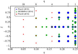
The accuracy of the new BAM simulations was discussed in some detail in Paper 1. In this work we are interested in constructing accurate waveform models for GW astronomy with aLIGO and AdV. In that context, an important accuracy measure is the mismatch between the waveforms with respect to the aLIGO noise spectrum. We calculate the mismatch between the numerical waveforms following the procedure outlined in Sec. II.2; in particular, we take into account the inspiral signal power, allowing us to calculate mismatches for low-mass systems, and reliably infer the (typically larger) mismatches in these systems due to any errors in the merger-ringdown waveforms. This procedure tends to estimate larger mismatches than integrating Eq. (8) over only the frequency range of the NR waveforms, as in, e.g., Ref. Hinder et al. (2013), and is a more conservative estimate of the mismatch error in the NR waveforms.

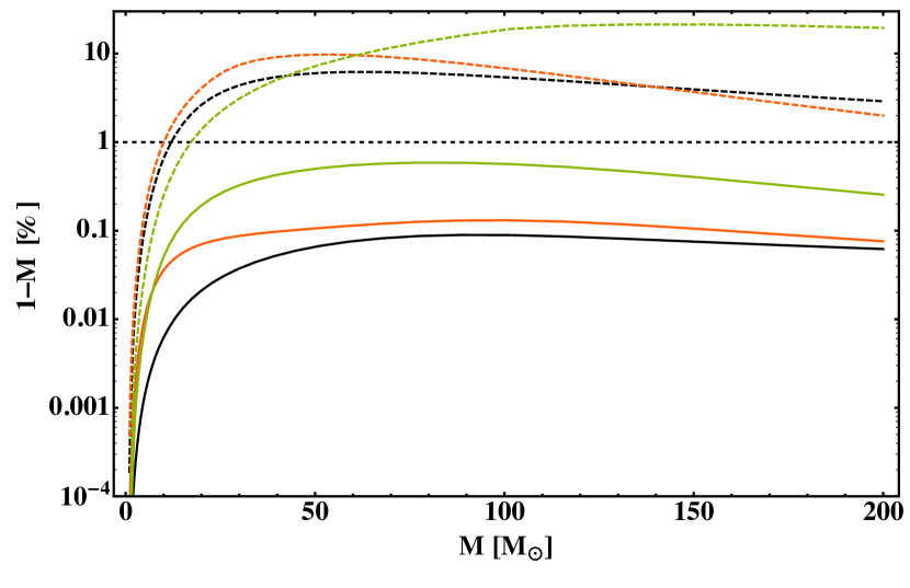
We consider the effect of two sources of error on the mismatch: the errors due to (1) finite numerical resolution, and (2) finite waveform extraction radius. In all cases we have found the overall mismatch error from these sources to be $<0.5$%. Here we focus on two configurations, $q=4$, $\chi_{1}=\chi_{2}=\hat{\chi}=0.75$ (A10), and nonspinning $q=18$ (A18).

Figure 2: Mismatch error due to numerical resolution, for the $q=4$, $\chi_{1}=\chi_{2}=\hat{\chi}=0.75$ (black lines) and non-spinnning $q=18$ simulations (orange lines). The solid black line shows the mismatch between waveform $q=4$ 112- and 96-point simuations, and the dashed black line shows the mismatch between the 96- and 80-point simulations. For the $q=18$ configuration, the solid orange line shows the mismatch between the 144- and 120-point simulations, and the dashed orange line shows the mismatch between the 144- and 96-point simulations (see text).

Figure 3: Mismatch errors due to finite-radius waveform extraction for the 120-point simulations of the same $q=4$ case as in Fig. 2. Mismatches are between the $R_{ex}=100\,M$ waveform and those extracted at $R_{ex}=\{50,60,70,80,90\}\,M$ (from top to bottom).

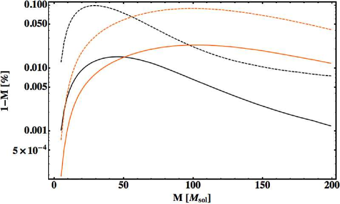
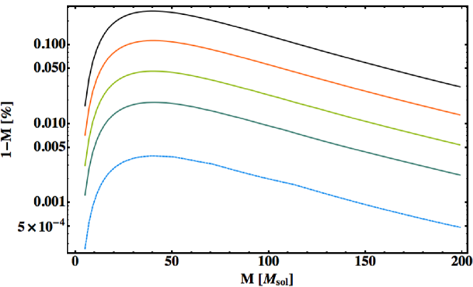
Fig. 2 shows the mismatch error due to numerical resolution. In the $q=4$ configuration, the reference simulation uses a base grid size of $112^{3}$ points, with the finest grid spacing being $h_{\rm min}=M/230$. Comparisons are made against simulations with the same resolution, but a base grid size of $96^{3}$ points, and an $80^{3}$ simulation with the resolution scaled to give the same physical grid sizes as in the $96^{3}$ simulation. The solid black line shows the mismatch between the $112$-point and $96$-point simulations, i.e., simulations where only the physical grid sizes were changed. This change introduces a mismatch error of at most $\sim 0.01$%. The dashed black line shows the mismatch between the $112$-point and $80$-point simulations, i.e., both the physical grid sizes and the numerical resolution have been reduced. Here the mismatch difference is at most $\sim 0.1$%.

The orange lines show the mismatch between the $q=18$ waveforms, with grid sizes of $96^{3}$, $120^{3}$ and $144^{3}$ points. These three simulations constitute a convergence series, and we have shown in Paper 1 that they exhibit evidence of sixth-order convergence. The solid orange line shows the mismatch between the $144^{3}$ and $120^{3}$ simulations, and the dashed orange line shows the mismatch between the $144^{3}$ and $96^{3}$ simulations. The higher mismatches at high mass, compared to the $q=4$ configuration, suggests that the merger-ringdown errors are larger in this case, although their effect on the mismatches at lower masses is comparable. We again conclude that the waveforms are accurate to well within our 1% criterion.

Although the convergence of our simulations is in general unclear, we typically find that our 80-point simulations are not in the convergence regime, and are much less accurate than higher-resolution simulations. We therefore expect that if the mismatch between the 112-point and 80-point simulations is no larger than 0.1%, then the mismatch between the 96- or 112-point simulations and the continuum limit will be lower than this; it will certainly be lower than the 1% accuracy requirement that we place on our model.

Fig. 3 shows the mismatch between waveforms extracted at different radii. The waveforms were extracted at $R_{ex}=\{50,60,70,80,90,100\}\,M$, and the mismatch calculations are performed against the $R_{ex}=100\,M$ waveforms. We expect the error to fall of as $\sim 1/R_{ex}$, and in general we observe this for our simulations, but only for $R_{ex}\gtrsim 60\,M$. Since even the $R_{ex}=50\,M$ waveform has a mismatch of only $\sim 0.3\%$ with the $R_{ex}=100\,M$ waveform, and assuming a $1/R_{ex}$ fall-off in waveform extraction error, we expect that the contribution of this error to the $R_{ex}=100\,M$ waveforms is less than 0.1%.

Based on this analysis, we conclude that our simulations are well within the accuracy requirements to construct a waveform model with an overall mismatch error of $\lesssim 1$%.

#	Code/ID	q	$\eta$	$\chi_{1}$	$\chi_{2}$	$\hat{\chi}$	$M_{f}$	$a_{f}$	$Mf_{\text{RD}}$	$Mf_{\text{hyb}}$	$N_{\rm GW,NR}$
A1	SXS:BBH:0156	1.	0.25	-0.95	-0.95	-0.95	0.9681	0.3757	0.0713	0.00522	22
A2	SXS:BBH:0151	1.	0.25	-0.6	-0.6	-0.6	0.9638	0.4942	0.0764	0.00517	26
A3	SXS:BBH:0001	1.	0.25	0.	0.	0.	0.9516	0.6865	0.0881	0.00398	54
A4	SXS:BBH:0152	1.	0.25	0.6	0.6	0.6	0.9269	0.8578	0.1083	0.00501	42
A5	SXS:BBH:0172	1.	0.25	0.98	0.98	0.98	0.8892	0.9470	0.1328	0.00497	48
A6	BAM	4.	0.16	-0.75	-0.75	-0.75	0.9846	0.0494	0.0614	0.00713	15
A7	BAM	4.	0.16	-0.5	-0.5	-0.5	0.9831	0.1935	0.0649	0.00716	18
A8	SXS:BBH:0167	4.	0.16	0.	0.	0.	0.9779	0.4715	0.0743	0.00665	28
A9	BAM	4.	0.16	0.5	0.5	0.5	0.9674	0.7377	0.0906	0.00811	26
A10	BAM	4.	0.16	0.75	0.75	0.75	0.9573	0.8628	0.1054	0.00818	30
A11	BAM	8.	0.099	-0.85	-0.85	-0.85	0.9898	-0.3200	0.0546	0.00918	8
A12	SXS:BBH:0064	8.	0.099	-0.5	0.	-0.458	0.9923	-0.0526	0.0589	0.00632	36
A13	SXS:BBH:0063	8.	0.099	0.	0.	0.	0.9894	0.3067	0.0677	0.00623	49
A14	SXS:BBH:0065	8.	0.099	0.5	0.	0.458	0.9846	0.6574	0.0838	0.00615	66
A15	BAM	8.	0.099	0.85	0.85	0.85	0.9746	0.8948	0.1087	0.01580	15
A16	BAM	18.	0.05	-0.8	0.	-0.77	0.9966	-0.5311	0.0514	0.01035	14
A17	BAM	18.	0.05	-0.4	0.	-0.385	0.9966	-0.1877	0.0563	0.01283	15
A18	BAM	18.	0.05	0.	0.	0.	0.9959	0.1633	0.0633	0.01284	13
A19	BAM	18.	0.05	0.4	0.	0.385	0.9943	0.5046	0.0745	0.00916	23

Table 1: Hybrid waveform configurations used to calibrate the PhenomD model. For each configuration we list both the mass ratio $q$ and symmetric mass ratio $\eta$, along with the spins $\chi_{1}$ and $\chi_{2}$ and the reduced-spin combination, $\hat{\chi}$, which follows from Eq. (4). The final BH has mass $M_{f}$ and dimensionless spin $a_{f}$, and the ringdown signal has frequency $Mf_{\rm RD}$. The frequency $Mf_{\text{hyb}}$ marks the midpoint of the transition region between SEOBv2 inspiral and NR data. The approximate number of NR GW cycles in each hybrid is given by $N_{\rm GW,NR}$.

IV Choice of inspiral approximant

The early, gradual inspiral of compact binaries and the GWs they emit can be accurately modeled by expanding the energy and flux of the system into a PN series. Depending on how the underlying equations are formulated and solved, there is a variety of PN approximants, each consistent with the others when truncated at the same expansion order. However, as every approximant is formulated with different, mostly implicit, assumptions of how higher order terms are treated, the GW signals they predict can differ considerably, especially towards higher mass ratios, increased spin magnitudes and for increasing orbital frequencies Hannam et al. (2008); Buonanno et al. (2009b); Hannam et al. (2010a); Ohme et al. (2011); MacDonald et al. (2011, 2013); Nitz et al. (2013). There are sophisticated methods that aim to improve the convergence and accuracy of PN-based approximants, and one of the most successful approaches is the mapping to an EOB system Buonanno and Damour (1999, 2000); Damour (2001).

In the construction of a complete waveform model we face the following two issues. First, we need to pick one approximant that, to our current knowledge, models the inspiral most accrately. Second, this inspiral description has to be complemented by NR-based information about the merger and ringdown. We briefly summarize our strategy to address both issues below and give references to the following sections that describe our reasoning in more detail.

Recent studies have indicated that among the family of non-precessing inspiral approximants, the EOB approximant by Tarachini et al. Taracchini et al. (2014a) shows the most consistent agreement with NR simulations within the calibration range of the model Szilágyi et al. (2015); Kumar et al. (2015). In Paper 1, we have performed an independent consistency test between inspiral approximants and our set of NR data and confirmed this conclusion. (Note that the most recently calibrated version of a non-precessing EOB model Nagar et al. (2015) has not yet been included in any of these tests.) Hence, we used the Tarachini et al. model (dubbed SEOBNRv2 in the publicly available LIGO software library The LIGO Scientific Collaboration (2015)) as our target inspiral approximant, albeit in its original, uncalibrated form that does not include NR fitted corrections (we refer to this form as as SEOBv2). Specifically, this involves calculating the SEOBNRv2 waveforms with all of the NR calibration terms set to zero, to provide an “uncalibrated” SEOBv2 calculation of the inspiral waveform.

We do so because our goal is to explore an alternative modeling approach that is independent of previous NR-informed EOB tuning. In particular, we performed dedicated NR simulations outside the calibration range of SEOBNRv2, and instead of inheriting higher-order corrections that were fitted in a smaller parameter space region, we prefer to use the uncalibrated EOB model purely in the inspiral regime and hybridize it with NR data of the merger and ringdown.

We are naturally limited by the lengths of the NR waveforms, which are different for every simulation. Previous studies of NR waveform length requirements have suggested that PN inspiral waveforms up to 5-10 orbits before merger are sufficiently accurate for detection purposes Hannam et al. (2010b); Ohme et al. (2011); many more orbits are needed to fulfil more stringent accuracy requirements MacDonald et al. (2011, 2013); Damour et al. (2011); Boyle (2011), especially in the high-mass-ratio and high-spin regime that we are covering. Many of our NR waveforms are too short to allow that. However, previous studies estimated the accuracy of PN approximants based on the differences between all available approximants at 3.5PN order (with highest spin corrections at 2.5PN order at that time). One might argue that the EOB approach is more accurate, and therefore comparisons between PN waveforms exaggerate the uncertainty in our best current models. On the other hand, without fully general-relativistic results to compare to, one might be sceptical of good agreements between alternative EOB waveforms that are very similar by construction.

Nevertheless, given that we can join EOB with our NR data in a much more robust manner than any of the PN approximants (see Sec. II of Paper 1 for our full analysis), we trust that they provide a reasonably accurate description of the inspiral up to the point where NR data take over. At what frequency this switch from EOB to NR happens depends on the length of the individual NR simulations. We note that the lowest common starting frequency of our NR waveforms is $Mf\sim 0.018$, and this is where we begin our phenomenological merger-ringdown model. Note, however, that our hybridization procedure ensures that the maximum amount of NR information is used in every point of the parameter space to inform both the inspiral and merger-ringdown part of our model.

V Model of the NR regime (Region II)

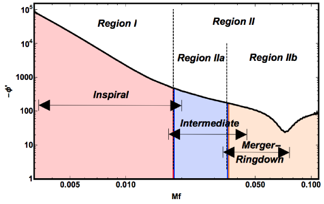
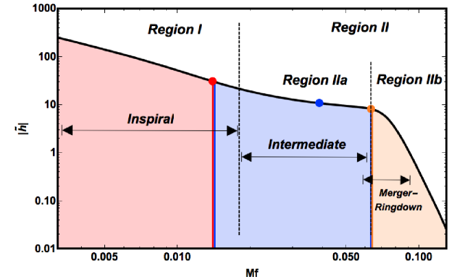
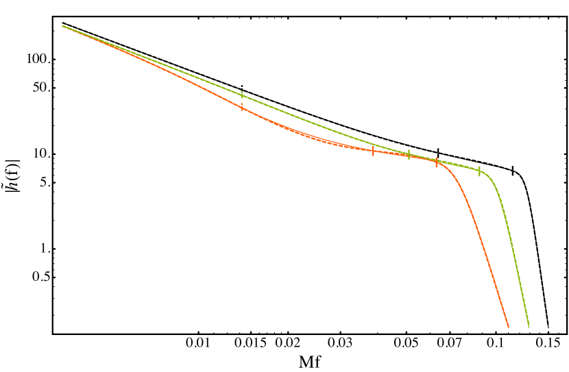
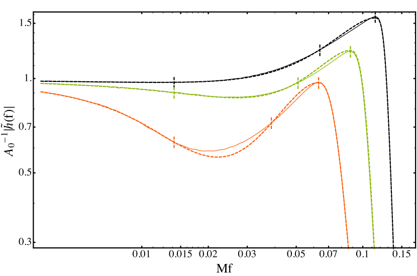
We model separately three frequency regions of the waveforms. These are indicated in Fig. 4. Region I is defined to be the portion of the hybrid that contains the optimal blend of NR and SEOBv2 data, Region II is the portion of the hybrid that contains purely NR data and corresponds to frequencies $Mf\geq 0.018$. This region is further sub-divided into two regions, Regions IIa and IIb. These divisions correspond to the intermediate and merger-ringdown models for both the amplitude and phase.

The figures indicate both the frequency ranges over which the three parts are connected, but also the ranges that are used to calibrate the model’s coefficients to the hybrid data. These regions are in general slightly larger than those used when piecing together the final model.

We will refer to other features of these figures in the forthcoming sections.

Figure 4: Phase derivative $-\phi^{\prime}(f)\equiv-\partial\phi(f)/\partial f$ (upper panel) and amplitude (lower panel) for the $q=1$, $\chi_{1}=\chi_{2}=-0.95$ configuration. The frequency ranges that were used in the fits for each section are shown as black double-ended arrows. For reference, the frequency $Mf=0.018$ is marked with a black dashed line. Shaded regions illustrate the boundaries between the different regions when constructing the full IMR waveform. The ringdown frequency for this case is $Mf=0.071$.

V.1 From PhenomC to PhenomD

The merger-ringdown portion of the phase was modelled in PhenomC Santamaría et al. (2010) using the ansatz,

$$\begin{split}\psi^{22}_{\rm PM}(f)&=\frac{1}{\eta}\left(\alpha_{1}f^{-5/3}+\alpha_{2}f^{-1}\right.\\ &\left.+\alpha_{3}f^{-1/3}+\alpha_{4}+\alpha_{5}f^{2/3}+\alpha_{6}f\right).\end{split}$$ (11)

The phase was fit over the frequency range $[0.1,1]f_{\rm RD}$. The reference phase and time of the fit are given by the coefficients $\alpha_{4}$ and $\alpha_{6}$. At the ringdown frequency $f_{\rm RD}$ the phase was smoothly connected to a linear function, $\psi^{22}_{\rm RD}(f)=\beta_{1}+\beta_{2}f$, using a $\tanh$ transition function.

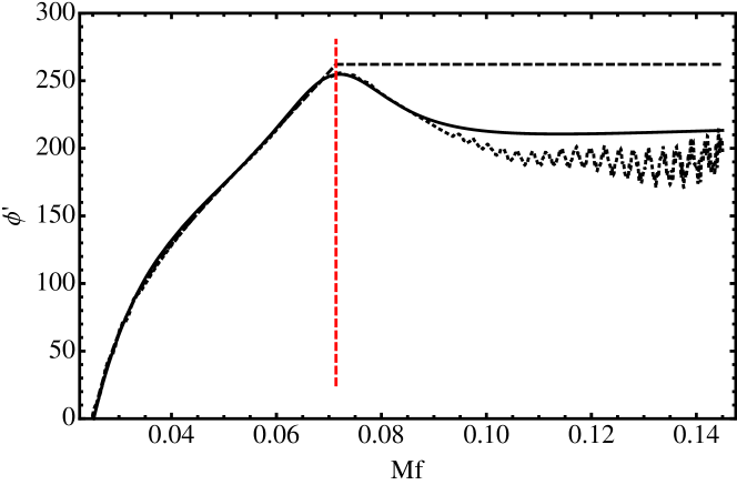
We now aim to model the merger-ringdown phase of the NR waveforms only from $Mf=0.018$, to ensure that we include only NR information in this part of the model. Fig. 5 shows the derivative of the frequency-domain phase for the configuration $q=1$, $\chi_{1}=\chi_{2}=-0.95$. The dashed line shows a fit to the phase using the procedure described above; beyond the ringdown frequency $Mf_{\rm RD}=0.071$ the derivative of the phase is constant, and in this example the transition is only piecewise continuous. We see that, while Eq. (11) is able to accurately reproduce the phase up to the ringdown frequency, the linear approximation at higher frequencies is crude.

The solid line in Fig. 5 shows a fit to the phase following the procedure we use to construct PhenomD, which was motivated in detail in Paper 1, and is also described in Sec. V.2.1 below. This accurately reproduces the main features of the phase derivative in the vicinity of the ringdown frequency. There is some disagreement at higher frequencies, but we note that the accuracy of the NR data typically degrades at these frequencies, and the true behaviour of $\phi^{\prime}(f)$ is not clear.

Figure 5: Phase derivative $\phi^{\prime}(f)$ for the $q=1$, $\chi_{1}=\chi_{2}=-0.95$ configuration. The numerical data (dotted) show a distinctive extremum at the ringdown frequency, $Mf_{\rm RD}=0.071$, indicated by a vertical dashed line. A fit that follows an approach similar to that used for PhenomC (dashed) is only a crude approximation to the phase for $f>f_{\rm RD}$, whereas the approach used for the PhenomD model (solid) accurately models the phase into the ringdown.

In the next section we describe the methodology used to produce models of the phase and amplitude for the late inspiral, merger and ringdown parts of the waveform, i.e., those frquencies for which we have NR data. These we have denoted Region II; see Fig. 4. We assume that we have a valid inspiral approximant that we can join to our NR-based Region II model to construct a full IMR waveform model. The construction of a suitable inspiral model (Region I) is given in Sec. VI.

Our current construction requires that the starting frequency of the Region II model must be consistent for all waveforms. This imposes the constraint that the starting frequency of the NR-based Region II model is the lowest common GW frequency for which we have NR data, $Mf\sim 0.018$. This is purely based on the available NR data and could in principle be pushed towards lower frequencies given longer waveforms.

V.2 Phase

To produce a robust model there are two key requirements: (1) the ansatz must fit the data well, i.e., the fits have small residuals to the data, and (2) the choice of ansatz should ideally be chosen to in such a way that the coefficients vary smoothly across the parameter space, to enable an accurate parameter-space fit in the final model.

We find that a simple approach is to split Region II into an intermediate (Region IIa) and merger-ringdown (Region IIb) part, and model them separately, as shown in Fig. 4.

The detailed features of the phase through Region II are most apparent when we consider the derivative of the phase, $\partial\phi/\partial f\equiv\phi^{\prime}(f)$. For this reason we first model $\phi^{\prime}$, and then integrate the resulting expression to produce the final phase model. We also note that the overall $1/\eta$ dependence in the inspiral, Eq. (27), also holds for the merger and ringdown, and so all of our primary fits are to $\eta\phi^{\prime}$.

V.2.1 Region IIb - merger-ringdown

An example of the derivative of the phase, $\phi^{\prime}$ is shown in Fig. 4 for a binary with $q=1$, $\chi_{1}=\chi_{2}=-0.95$. As described in Paper 1, we propose the following ansatz to model this functional form,

$$\phi^{\prime}_{\text{MR}}=\alpha_{1}+\alpha_{2}f^{-2}+\alpha_{3}f^{-1/4}+\frac{a}{b^{2}+(f-f_{0})^{2}}.$$ (12)

The last term models the ‘dip’ in Fig. 4. The location of the minimum is given by $f_{0}$, while $a$ is the overall amplitude of the dip and $b$ is the width. We find that the frequency location of the dip is very close to the final BH’s ringdown frequency, $f_{\rm RD}$ (they agree within our uncertainty in calculating $f_{\rm RD}$), and that the ringdown damping frequency $f_{\rm damp}$ is a good approximation to our best fit of the width. These quantities are calculated from our final mass and spin fits. For these reasons the ansatz that we use in practice is,

$$\eta\,\phi^{\prime}_{\text{MR}}=\alpha_{1}+\alpha_{2}f^{-2}+\alpha_{3}f^{-1/4}+\frac{\alpha_{4}f_{\text{damp}}}{f_{\text{damp}}^{2}+(f-\alpha_{5}f_{\text{RD}})^{2}}.$$ (13)

We find that the parameter $\alpha_{5}$ is in the range $[0.98,1.04]$. The power law terms account for the overall trend of the data, and its behaviour at lower frequencies. The constant term translates into a time shift in the overall phase, which will be determined by the continuity requirements of the final IMR phase; see Sec. VIII. The phase derivative data are fit to Eq. (13) over the frequency range $\left[0.45,1.15\right]f_{\text{RD}}$. The upper frequency $1.15f_{\text{RD}}$ approximates the highest frequency for which we have clean NR data. This fitting window was chosen to have some overlap between the intermediate phase model, as indicated in Fig. 4.

The merger-ringdown phase is given by the integral of Eq. (13),

$$\begin{split}\phi_{\text{MR}}&=\frac{1}{\eta}\left\{\alpha_{0}+\alpha_{1}f-\alpha_{2}f^{-1}+\frac{4}{3}\alpha_{3}f^{3/4}\right.\\ &\left.+\,\,\alpha_{4}\tan^{-1}\left(\frac{f-\alpha_{5}f_{\text{RD}}}{f_{\text{damp}}}\right)\right\}\,.\end{split}$$ (14)

For the full IMR phase we use the above fit for frequencies larger than $0.5\,f_{\text{RD}}$. At lower frequencies we find that $\eta\,\phi^{\prime}$ is fit better by $\sim 1/f$ and we model this region (IIa) separately.

The phase offset that appears as a constant of integration $\alpha_{0}$, and the time-shift term $\alpha_{1}$, will both be determined in the final model by requiring a smooth connection with the phase from Region IIa.

Figure 6: Examples of the merger-ringdown (Region IIb) model for three $q=18$ configurations where the spin on the large BH is $\chi_{1}=\{+0.4,0,-0.8\}$ and three equal-spin $q=1$ configurations ($\chi_{1,2}=+0.98,0,-0.95$). The configurations are ordered top to bottom in the figure. The left panel shows the hybrid data, best-fit and final-model predictions over Region IIb. The right panel shows the difference between the hybrid data and the best-fit (dashed line) and between the hybrid data and the final model (solid line).

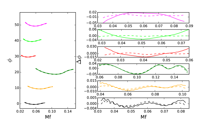
Examples of the results are shown in Fig. 6 for six configurations at the edges of our calibration parameter space. These are equal-spin $q=1$ waveforms with spins $\hat{\chi}=\{-0.95,0,0.98\}$ and $q=18$ waveforms with spins on the larger BH of $\chi_{1}=\{-0.8,0,0.4\}$ (the second BH has no spin). In addition to demonstrating that both the ansatz and the final model capture the data well, the figure also illustrates the large differences in the frequency range of the merger-rigndown at different points in the parameter space.

V.2.2 Region IIa - intermediate

To bridge the gap between the lowest common frequency of the NR data and the Region IIb merger-ringdown model, i.e., over the frequency range $Mf\in\left[0.018,0.5f_{\text{RD}}\right]$, we use the following ansatz,

$$\eta\,\phi^{\prime}_{\text{Int}}=\beta_{1}+\beta_{2}f^{-1}+\beta_{3}f^{-4}\,.$$ (15)

The behaviour of the data over this frequency range is predominately proportional to $1/f$. This is not sufficient at higher mass ratios and high anti-aligned spins, where $f_{\text{RD}}$ can be approximately half that of the equal mass non-spinning case. We find that the additional $f^{-4}$ term fits the data well across the entire parameter space. The intermediate (Region IIa) ansatz is used over the frequency interval $[0.018,0.5f_{\text{RD}}]$, but we found that the best results were obtained if the data were fit over $[0.017,0.75f_{\text{RD}}]$.

Once again the phase is obtained by integrating Eq. (15),

$$\phi_{\text{Int}}=\frac{1}{\eta}\left(\beta_{0}+\beta_{1}f+\beta_{2}\,\text{Log}(f)-\frac{\beta_{3}}{3}f^{-3}\right)\,.$$ (16)

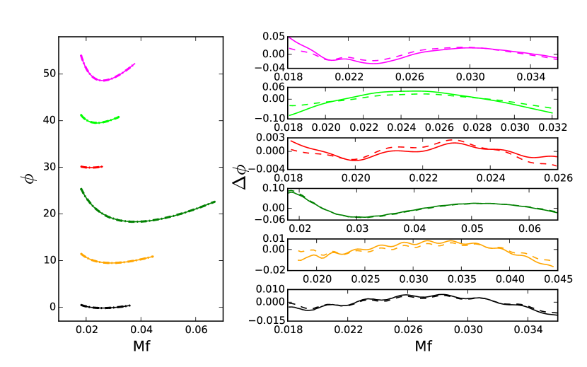
As in Region IIb, the phase-shift due to the constant of integration $\beta_{0}$, and the time-shift term $\beta_{1}$, will be fixed by requiring a smooth connection to the Region I phase. The results for the corner cases are shown in Fig. 7.

Figure 7: The same configurations and layout as in Fig. 6, but now showing phase over the intermediate region (IIa).

This completes the modelling of the phase over the frequencies for which we have NR data, Region II. We will now consider the signal amplitude over the same region, before moving on to the inspiral, Region I.

V.3 Amplitude

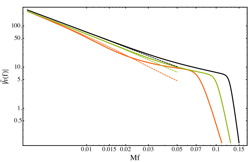
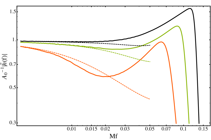
When we perform the fits to the amplitude across Region I and Region II, we first factor out the leading order PN $f^{-7/6}$ behaviour. The resulting data tend to unity as the frequency tends to zero, and as with the use of the phase derivative, allows us to identify and model detailed features of the amplitude behaviour; see Fig. 8, which shows both amplitude for PN inspiral waveforms, and for the full hybrids.

The normalisation is given by,

$$\lim_{f\to 0}\left[f^{7/6}\,A_{\text{PN}}(f)\right]\rightarrow\sqrt{\frac{2\,\eta}{3\,\pi^{1/3}}},$$ (17)

and our normalisation factor is therefore,

$$A_{0}\equiv\sqrt{\frac{2\,\eta}{3\,\pi^{1/3}}}f^{-7/6}.$$ (18)

V.3.1 Region IIb - merger-ringdown

In all previous phenomenological models Ajith et al. (2007, 2011); Santamaría et al. (2010), the ringdown amplitude has been modelled with a Lorentzian function, which is the Fourier transform of the (two-sided) exponential decay function. The Fourier transform of the full IMR data instead exhibit an exponential decay, as discussed in Paper 1. The amplitude in Region IIb is fit over the frequency range $Mf\in\left[1/1.15,1.2\right]f_{\text{RD}}$ using the following ansatz,

$$\frac{A_{\text{MR}}}{A_{0}}=\gamma_{1}\frac{\gamma_{3}f_{\text{damp}}}{(f-f_{\text{RD}})^{2}+(\gamma_{3}f_{\text{damp}})^{2}}e^{-\frac{\gamma_{2}(f-f_{\text{RD}})}{\gamma_{3}f_{\text{damp}}}}\,.$$ (19)

The coefficient $\gamma_{1}\in[0.0024,0.0169]$ determines the overall amplitude of the ringdown. We expect that the frequency width and location of the amplitude peak can be inferred from the remnant BH parameters, which motivates the appearance of the ringdown damping frequency $f_{\rm damp}$ in Eq. (19). In practice we find that the width is increased by the factor $\gamma_{3}\in[1.25,1.36]$, and the decay rate $1/(f_{\text{damp}}\gamma_{3})$ is modified by the factor $\gamma_{2}\in[0.54,1.0339]$.

If we used only the Lorentzian part of Eq. (19), the amplitude peak would be located at $f_{\rm RD}$. With the additional exponential factor, the peak is located at

$$f_{\rm peak}=\left|f_{\text{RD}}+\frac{f_{\text{damp}}\gamma_{3}\left(\sqrt{1-\gamma_{2}^{2}}-1\right)}{\gamma_{2}}\right|.$$ (20)

V.3.2 Region IIa - intermediate

Figure 8: Hybrid Fourier domain amplitude for three equal mass cases $q=1$, $\chi_{1}=\chi_{2}=0.98$, $\chi_{1}=\chi_{2}=0$ and $\chi_{1}=\chi_{2}=-0.95$, indicated by black, orange and green lines respectively. The PN prediction is shown as dashed lines. The left panel shows the full fourier domain amplitude, while the right panel shows the fourier domain amplitude but rescaled by $A_{0}^{-1}$, Eq. (18).

We now consider the intermediate region (IIa) between the end of the inspiral region (I) and the start of the merger-ringdown region (IIb).

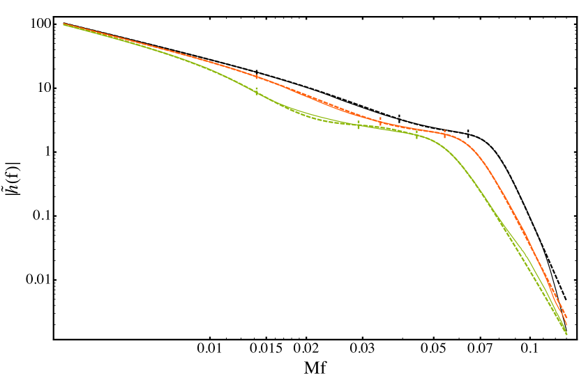
Fig. 8 shows the TaylorF2 inspiral amplitude in comparison to the amplitude in the hybrid data. In some cases, we see that we can model the intermediate (Region IIa) amplitude by simply smoothly connecting regions I and IIb. For example, we could fit the four coefficients of a third-order polynomial by matching the value of the amplitude and its derivative at the end of the Region I (nominally $Mf=0.018$) and at the beginning of Region IIb, $f_{\rm peak}$.

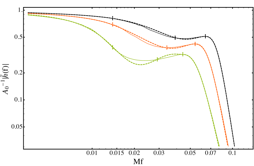
In other cases, however, we see that the rescaled amplitude will have a minimum in the intermediate region, and a naive connection of the inspiral and merger-ringdown regions would not in general locate this minimum correctly.

For this reason, we model the intermediate amplitude with a fourth-order polynomial. Four of the coefficients are fixed (as above), by matching the value and derivative of the amplitude at the endpoints of our intermediate fit. The lower frequency is chosen as $Mf_{1}=0.014$, i.e., slightly before the end of the inspiral at $Mf=0.018$, and the upper frequency is $f_{3}=f_{\rm peak}$. The fifth coefficient is determined by the value of amplitude of the NR waveform at the frequency mid-way between the two, $f_{2}=(f_{1}+f_{3})/2$.

In practice, the amplitude values and derivatives at the endpoints are given by the models for Region I and Region IIB. The only additional piece of information that needs to be modelled from the NR data is the value of the amplitude at $f_{2}$. We find that this can be accurately modelled across the parameter space by a polynomial ansatz in ($\eta,\hat{\chi}$), as will be described in Sec. VII.

This collocation method is similar to that used in spectral methods. Given an ansatz with $n$ free coefficients we require $n$ pieces of information from the data to constrain the ansatz and solve the system. In this case we use the value of the function at three points, and the derivative at two points. The intermediate ansatz is given by

$$A_{\text{Int}}=A_{0}\left(\delta_{0}+\delta_{1}f+\delta_{2}f^{2}+\delta_{3}f^{3}+\delta_{4}f^{4}\right),$$ (21)

and the $\delta_{i}$ coefficients are the solution to the system of equations,

$$A_{\text{Int}}(f_{1}) = v_{1},$$ (22)

$$A_{\text{Int}}(f_{2}) = v_{2},$$ (23)

$$A_{\text{Int}}(f_{3}) = v_{3},$$ (24)

$$A^{\prime}_{\text{Int}}(f_{1}) = d_{1},$$ (25)

$$A^{\prime}_{\text{Int}}(f_{3}) = d_{3}.$$ (26)

The frequencies and values are given in Tab. 2.

Collocation Point (Mf)	Value	Derivative
$f_{1}=0.014$	$v_{1}=A_{\text{Ins}}(f_{1})$	$d_{1}=A^{\prime}_{\text{Ins}}(f_{1})$
$f_{2}=(f_{1}+f_{3})/2$	$v_{2}=A_{\text{Hyb}}(f_{2})$
$f_{3}=f_{\text{peak}}$	$v_{3}=A_{\text{MR}}(f_{3})$	$d_{3}=A^{\prime}_{\text{MR}}(f_{3})$

Table 2: Locations of the collocation points, $f_{1},f_{2},f_{3}$, and the corresponding values of the amplitude $A(f)$ and its derivative $A^{\prime}(f)$. All information comes from either the inspiral or merger-ringodwn models, except for the value $v_{2}$, which is read off the input waveform data.

The results of our amplitude model are shown in Figs. 9 and 10, which show the same equal-mass and $q=18$ cases as in Fig. 6. The left panels show the full signal amplitude, while the right panels show the amplitude scaled by the $f^{7/6}$ factor, Eq. 18.

The scaled plots indicate that the weakest part of the model is that which describes the intermediate Region IIa amplitude. This is because the minimum that we see in the scaled figures (those in the right panels) is captured only through the value of the amplitude at the frequency in the middle of Region IIa. If we were in addition to model the frequency at which the minimum occurs, and prescribe the amplitude value there, the model may perform better. We could also, of course, add further collocation points. However, we can see from the full unscaled amplitude (the left panels) that the amplitude is nonetheless very accurately represented, and in addition, small variations in the amplitude play a far smaller role in GW applications (both searches and parameter estimation) than the GW phase.

Figure 9: Hybrid and model Fourier-domain amplitude for three equal-mass configurations, $\chi_{1}=\chi_{2}=0.98$, $\chi_{1}=\chi_{2}=0$ and $\chi_{1}=\chi_{2}=-0.95$, indicated by black, orange and green lines respectively. The hybrid data are shown by solid lines, and the PhenomD model by dashed lines. The left panel shows the full Fourier-domain amplitude, while the right panel shows the Fourier-domain amplitude but rescaled by $A_{0}^{-1}$, Eq. (18). The short vertical dashed lines mark the three frequency points in Tab (2), while the lines at lower and higher frequency coincide with the transition points between regions I and IIa and between regions IIa and IIb respectively.

Figure 10: The same quantities as in Fig. 9, but now for three $q=18$ configurations, $\chi_{1}=0.4,\chi_{2}=0$, $\chi_{1}=\chi_{2}=0$ and $\chi_{1}=-0.8,\chi_{2}=0$.

VI Inspiral model (Region I)

We now turn our attention to modelling Region I, i.e., the inspiral portion of the waveform, below the frequency $Mf=0.018$; see Fig. 4.

The non-spinning Ajith et al. (2007) and the first aligned-spin Ajith et al. (2011) phenomenological models used a PN-like ansatz for the inspiral phase, calibrated against PN+NR hybrids. In the PhenomC model Santamaría et al. (2010), the TaylorF2 phase was used for the equivalent of Region I; in that model the inspiral region ended at $0.1f_{\text{RD}}$. For the parameter space covered by our new model, this would corresponds to frequencies between $Mf\sim 0.005$ and $Mf\sim 0.012$.

In Paper 1 we presented evidence that the uncalibrated SEOBv2 model is currently the inspiral approximant that is most consistent with NR data for the inspiral. In this section we construct a frequency domain model of the SEOBv2 inspiral, up to $Mf=0.018$, using our SEOBv2+NR hybrids. As discussed previously, we expect that the SEOBv2 model is sufficiently accurate up to this frequency, and very likely to higher frequencies, allowing us to match to our merger-ringdown model at significantly higher frequencies than was considered reasonable with the TaylorF2 approximant used for PhenomC.

Note that it is possible, in principle, to cover the parameter space with an arbitrarily high density of SEOBv2 waveforms, and use those to calibrate an inspiral model. In this paper, however, we use hybrid SEOBv2+NR waveforms and therefore calibrate the inspiral model to the same points in parameter space as used for the Region II merger-ringdown models.

VI.1 Phase

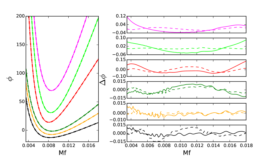
The inspiral portion $Mf\in[0.0035,0.018]$ of the hybrids can be accurately modelled with an ansatz consisting of the known TaylorF2 terms for the phase, augmented with the next four higher order PN terms, with their coefficients fit to the SEOBv2+NR hybrid data. We find that these higher order terms are enough to capture the EOB and NR data over this frequency range to a very high level of accuracy.

The full TaylorF2 phase is,

$$\phi_{\text{TF2}} = \,2\pi ft_{c}-\varphi_{c}-\pi/4$$ (27)

$$+\frac{3}{128\,\eta}(\pi fM)^{-5/3}\sum_{i=0}^{7}\varphi_{i}(\Xi)(\pi fM)^{i/3},$$

where $\varphi_{i}(\Xi)$ are the PN expansion coefficients that are functions of the intrinsic binary parameters. Explicit expressions are given in Appendix B. We incorporate spin-independent corrections up to 3.5PN order ($i=7$) Buonanno et al. (2009b); Blanchet (2014), linear spin-orbit corrections up to 3.5PN order Bohé et al. (2013) and quadratic spin corrections up to 2PN order Poisson (1998); Arun et al. (2009); Mikoczi et al. (2005). In re-expanding the PN energy and flux to obtain the TaylorF2 phase, we drop all quadratic and higher-order spin corrections beyond 2PN order as they would constitute incomplete terms in our description. With these choices, we are entirely consistent with the current state of the LIGO software library The LIGO Scientific Collaboration (2015). We note that we also constructed a full model that incorporated recently calculated higher-order terms, specifically quadratic spin terms at 3PN order Bohé et al. (2015) and cubic spin terms at 3.5PN order Marsat (2015), but we found no significant difference between both constructions.

Equation (27) includes both spins, $\chi_{1}$ and $\chi_{2}$, while our fit for the coefficients of additional terms will be parameterized only by $\hat{\chi}$. This means that the final phase expression will incorporate some effects from the spins of each BH, but, although the model is sufficiently accurate for use in GW astronomy applications across a wide range of the two-spin parameter space, it should not be considered an accurate representation of two-spin effects. We expect the model to be more than sufficient for searching for BH binaries with any BH spins within the calibration parameter space, or for estimation of the parameters $(M,\eta,\hat{\chi})$, but we do not recommend its use in, for example, theoretical studies of detailed double-spin effects in binaries.

The phase ansatz is given by,

$$\begin{split}\phi_{\text{Ins}}=&\phi_{\text{TF2}}(Mf;\Xi)\\ +&\frac{1}{\eta}\left(\sigma_{0}+\sigma_{1}f+\frac{3}{4}\sigma_{2}f^{4/3}+\frac{3}{5}\sigma_{3}f^{5/3}+\frac{1}{2}\sigma_{4}f^{2}\right).\end{split}$$ (28)

Note that to compute the phenomenological coefficients the fit is performed over the frequency range $Mf\in[0.0035,0.019]$ to achieve an optimal balance between goodness of fit and accuracy in reproducing phenomenological coefficients and to reduce boundary effects at the interface between Region I and Region IIa (i.e., $Mf=0.018$). In practice the fits were performed over the $\phi^{\prime}$ data, as with Region II above. We will see in Sec. IX.1 that this model also sufficiently accurately represents SEOBv2+NR hybrids down to much lower frequencies.

The results for the three example $q=1$ and $q=18$ configurations are shown in Fig. 11. We see that once again our ansatz accurately models the data, and that the Fourier-domain phase error is below 0.15 rad for the entire inspiral for the high-mass ratio configurations, while for the equal-mass configurations the phase error is typically an order of magnitude smaller.

Figure 11: The same analysis as in Figs. 6 and 7, but now for the inspiral model.

VI.2 Amplitude

Our model of the inspiral amplitude is based on a re-expanded PN amplitude, as discussed in Sec. IV of Paper 1. The base amplitude is given by,

$$A_{\text{PN}}(f)=A_{0}\sum_{i=0}^{6}\mathcal{A}_{i}(\pi f)^{i/3}\,,$$ (29)

where $A_{0}$ is the leading order $f^{-7/6}$ behaviour in Eq. (18). The higher order terms that we calibrate are the next natural terms in the PN expansion,

$$A_{\text{Ins}}=A_{\text{PN}}+A_{0}\sum_{i=1}^{3}\rho_{i}\,f^{(6+i)/3}.$$ (30)

VII Mapping the phenomenological coefficients to physical parameters

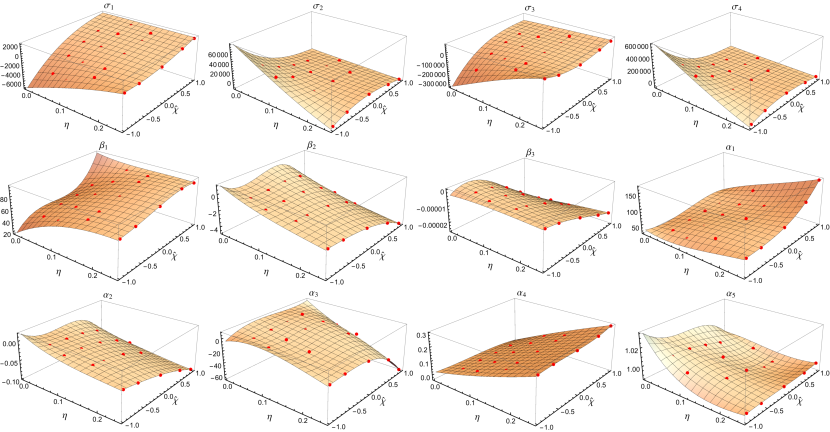
Our model has 11 amplitude and 14 phase coefficients. However four of the amplitude coefficients in Region IIa (Sec. V.3.2) and four of the phase coefficients $(\alpha_{0},\alpha_{1},\beta_{0},\beta_{1})$ across Region II (See Sec. VIII) are constrained analytically; there is only one time and phase-shift freedom for the full waveform. This leaves a total of 17 phenomenological parameters which need to be mapped on to the physical parameter space. We parametrise the phenomenological coefficients by two physical parameters, $(\eta,\chi_{\rm PN})$. Our model is also dependent on the total mass $M$ of the system through a trivial rescaling.

As in previous phenomenological models Ajith et al. (2007, 2011); Santamaría et al. (2010) we map the phenomenological coefficients in terms of polynomials of the physical parameters, up to second order in $\eta$ and third order in $\chi_{\rm PN}$, although in this work our polynomial ansatz is expanded around $\chi_{\rm PN}=1$. Note that in the fit across the parameter space we use the unscaled reduced-spin parameter $\chi_{\rm PN}$,

$$\begin{split}\Lambda^{i}=&\,\lambda^{i}_{00}+\lambda^{i}_{10}\eta\\ &(\chi_{\rm PN}-1)\left(\lambda^{i}_{01}+\lambda^{i}_{11}\eta+\lambda^{i}_{21}\eta^{2}\right)\\ &+(\chi_{\rm PN}-1)^{2}\left(\lambda^{i}_{02}+\lambda^{i}_{12}\eta+\lambda^{i}_{22}\eta^{2}\right)\\ &+(\chi_{\rm PN}-1)^{3}\left(\lambda^{i}_{03}+\lambda^{i}_{13}\eta+\lambda^{i}_{23}\eta^{2}\right)\,,\end{split}$$ (31)

where $\Lambda^{i}$ indexes both the amplitude and phase coefficients given by,

$$\Lambda^{i}=\big{\{}\underbrace{\{\rho_{j}\},\{v_{2}\},\{\gamma_{j}\}}_{\text{Amplitude Coefficients}},\underbrace{\{\sigma_{j}\},\{\beta_{j}\},\{\alpha_{j}\}}_{\text{Phase Coefficients}}\big{\}}\,.$$ (32)

The index $i\in\{1,2,3,4,5,6\}$ selects the coefficient vector for either amplitude or phase and model for Region I, IIa or IIb. Tab. 5 in Appendix C contains the values of all the mapping coefficients for each phenomenological parameter.

VIII Full IMR waveforms

By construction, all the regions of the amplitude and phase models are joined by $C(1)$-continuous conditions. This ensures the first derivative of the amplitude and phase at the boundary between the various regions, which are used in analytic calculations, are smooth. We assume that this is sufficient and simply join together the piecewise regions with step functions. Our step function is defined as

$$\theta(f-f_{0})=\left\{\begin{array}[]{lllll}-1,&&f<f_{0},\\ 1,&&f\geq f_{0},\\ \end{array}\right.$$ (35)

and,

$$\theta_{f_{0}}^{\pm}=\frac{1}{2}\left[1\pm\theta(f-f_{0})\right].$$ (36)

The full IMR phase is determined up to an arbitrary time- and phase shift. These shifts are absorbed into the constant and linear coefficients of the inspiral part $(\sigma_{0},\sigma_{1})$. The constant and linear coefficients of the Region IIa $(\alpha_{0},\alpha_{1})$ and IIb models $(\beta_{0},\beta_{1})$ are fixed by the requirement of $C(1)$ continuity.

The full IMR phase is given by the following equation

$$\Phi_{\text{IMR}}(f)=\phi_{\text{Ins}}(f)\,\theta_{f_{1}}^{-}+\theta_{f_{1}}^{+}\,\phi_{\text{Int}}(f)\,\theta_{f_{2}}^{-}+\theta_{f_{2}}^{+}\,\phi_{\text{MR}}(f)\,,$$ (37)

where $\phi_{\text{Ins}}$ is given by Eq. (28), $\phi_{\text{Int}}$ by Eq. (16), and $\phi_{\text{MR}}$ by Eq. (14), and the transition frequencies are $f_{1}=0.018$ and $f_{2}=0.5f_{\text{RD}}$. As noted previously, when evaluating the known PN part of $\phi_{\text{Ins}}$, given in Eq. (28), we use the full two spin dependence.

The full IMR amplitude is given by

$$A_{\text{IMR}}(f)=A_{\text{Ins}}(f)\,\theta_{f_{1}}^{-}+\theta_{f_{1}}^{+}\,A_{\text{Int}}(f)\,\theta_{f_{2}}^{-}+\theta_{f_{2}}^{+}\,A_{\text{MR}}(f)\,,$$ (38)

where $A_{\text{Ins}}$ is given by Eq. (30), $A_{\text{Int}}$ by Eq. (21), and $A_{\text{MR}}$ by Eq. (19), and where the transition frequencies are $f_{1}=0.014$ and $f_{2}=f_{\rm peak}$, Eq. (20). The amplitude is $C(1)$-continuous by construction. Once again, note that the base inspiral PN amplitude includes both spin contributions.

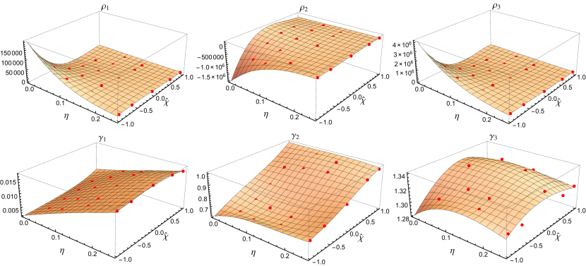
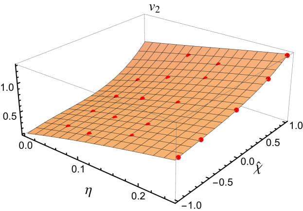
The phase and amplitude coefficients across the $(\eta,\hat{\chi})$ parameter space are shown in Figs. 12, 13 and 14. We see that in general the coefficients vary smoothly across the parameter space, and are captured well by our fits.

Figure 12: Phase coefficients for region I and II. The calibration points and the model, extrapolated to the boundary of the physical parameter space are shown.

Figure 13: Amplitude coefficients for region I and IIb. The calibration points and the model, extrapolated to the boundary of the physical parameter space are shown.

Figure 14: Intermediate (Region IIb) amplitude coefficient. The calibration points and the model, extrapolated to the boundary of the physical parameter space are shown.

IX Model Validation

To evaluate the accuracy of our model we compute the mismatch, defined in Sec. II.2, between the model and a set of hybrid waveforms, including the 19 waveforms used to calibrate the model (Tab. 1), and an additional 28 waveforms, listed in Tab. 3. The additional SpEC NR waveforms comprise most of the remaining aligned spin simulations in the public SXS catalogue SXS . The remaining NR waveforms were produced with BAM.

In this section we quantify the agreement for each of these waveforms against the PhenomD model. We also show (Sec. IX.3) that using additional waveforms in the calibration does not significantly change our model, and provide evidence that the set of waveforms we have chosen may be close to the minimal set necessary to accurately calibrate our model.

A further, complementary validation based on time-domain transformations is presented in Appendix A.

#	Code/ID	$q$	$\chi_{1}$	$\chi_{2}$
B1	SXS:BBH:0159	1.	-0.9	-0.9
B2	SXS:BBH:0154	1.	-0.8	-0.8
B3	SXS:BBH:0148	1.	-0.438	-0.438
B4	SXS:BBH:0149	1.	-0.2	-0.2
B5	SXS:BBH:0150	1.	0.2	0.2
B6	SXS:BBH:0170	1.	0.437	0.437
B7	SXS:BBH:0155	1.	0.8	0.8
B8	SXS:BBH:0153	1.	0.85	0.85
B9	SXS:BBH:0160	1.	0.9	0.9
B10	SXS:BBH:0157	1.	0.95	0.95
B11	SXS:BBH:0158	1.	0.97	0.97
B12	SXS:BBH:0014	1.5	-0.5	0.
B13	SXS:BBH:0008	1.5	0.	0.
B14	SXS:BBH:0013	1.5	0.5	0.
B15	SXS:BBH:0169	2.	0.	0.
B16	BAM	2.	0.5	0.5
B17	BAM	2.	0.75	0.75
B18	BAM	3.	-0.5	-0.5
B19	SXS:BBH:0036	3.	-0.5	0.
B20	SXS:BBH:0168	3.	0.	0.
B21	SXS:BBH:0045	3.	0.5	-0.5
B22	SXS:BBH:0031	3.	0.5	0.
B23	SXS:BBH:0047	3.	0.5	0.5
B24	BAM	4.	-0.25	-0.25
B25	BAM	4.	0.25	0.25
B26	SXS:BBH:0060	5.	-0.5	0.
B27	SXS:BBH:0056	5.	0.	0.
B28	SXS:BBH:0166	6.	0.	0.
B29	BAM	10.	0.	0.

Table 3: Additional waveforms used to verify the model, but not used in its calibration.

IX.1 Mismatches

In this section we compute the mismatch between PhenomD and all of the hybrid waveforms in Tabs. 1 and 3.

The model was calibrated to hybrid waveforms with a starting frequency of $Mf=0.0035$, but the waveforms from many astrophysical compact binaries will be detectable by aLIGO and AdV from much lower frequencies. We assume that the minimum mass for one of the compact objects is given by the typical mass of a neutron star i.e., $M_{\rm{NS}}\sim 1.4M_{\odot}$. The total mass of the binary can then be no lower than $M_{\rm{min}}=(q+1)M_{\rm{NS}}$ for configurations with mass-ratio $q$. Our goal is to produce a model that is accurate for binaries that can be detected from 10 Hz down to either $12\,M_{\odot}$ Buonanno et al. (2009b), or $M_{\rm min}$, if this exceeds $12\,M_{\odot}$, which is the case for systems with $q\gtrsim 8$. At 10 Hz, the waveform frequency of a $12\,M_{\odot}$ binary is $Mf\approx 0.0006$, and so in this section we compare our model to much longer hybrids that extend down to $Mf=0.0006$.

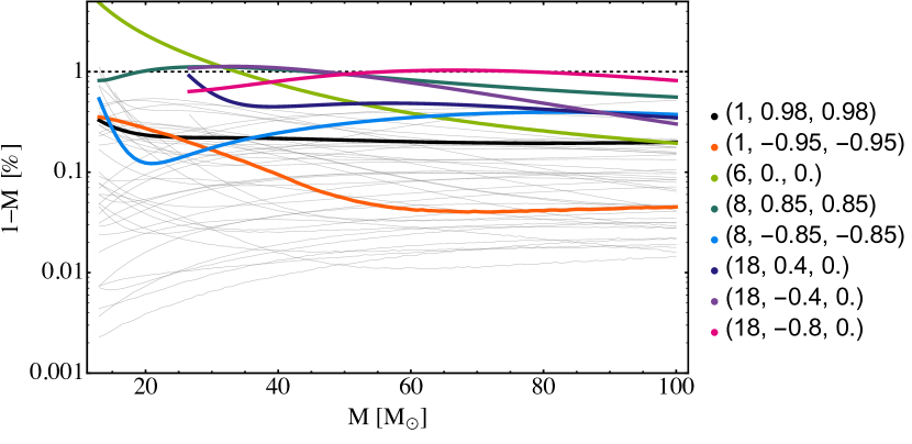
The results are presented in Fig. 15. The left panel uses the aLIGO design sensitivity zero-detuned, high-laser-power noise curve with $[f_{\rm min},f_{\rm max}]=[10,8000]$ Hz Shoemaker et al. (2010). The worst mismatch is for the $\{q,\chi_{1},\chi_{2}\}=\{6,0,0\}$ at low masses which tends towards a mismatch of 3% at $12\,M_{\odot}$. All other mismatches fall below 1% with the majority distributed around 0.1%. We note, however, that the fitting factors for the waveforms in the model (i.e., matches optimised over binary parameters, which is the relevant quantity for searches) are better than 0.999 in all cases we have considered. In particular, at low masses the mismatch between different options of inspiral approximant will be much larger than the mismatch between PhenomD and our hybrid waveforms; the dominant error is in our uncertainty of the true inspiral waveform, and not in our model; this will be made clearer in Sec. X.

Figure 15: Mismatches of the PhenomD model against all 48 available hybrid waveforms. The highlighted configurations are those closest to the edge of the $(\eta,\hat{\chi})$ parameter space as well as the case with the worst mismatch $(q,\chi_{1},\chi_{2})=(6,0.,0).$ The majority of cases show mismatches well below 1%. Left: Mismatches using the aLIGO design sensitivity noise curve (zdethp) with a lower frequency cut off of 10 Hz. Right: Early aLIGO noise curve with a 30 Hz cut off.

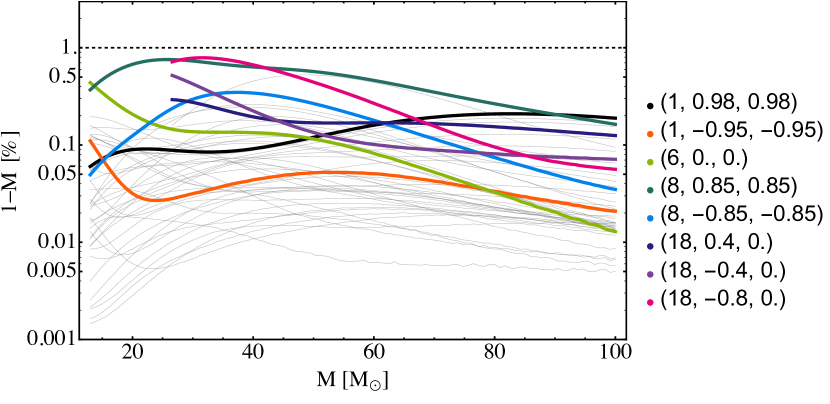
The right panel in Fig 15 shows the same calculation but using the predicted noise curve for early aLIGO science runs Aasi et al. (2013b), with a lower frequency cut-off of 30 Hz. Due to the change in shape of the noise curve and lower frequency cut-off the mismatches improve such that all mismatches are comfortably below 1%. This gives a more realistic idea of the performance of our model during the initial science run of the advanced detectors.

In both panels, the highlighted cases are those at the edges of the calibration region of parameter space. We note that the worst mismatches are for high mass ratios and large spins. This suggests the region of parameter space that requires the most improvement in future models — although it is clear that for all of these configurations the model is well within the accuracy requirements for the second-generation detectors.

IX.2 The effective spin approximation

The phenomenological fits to the waveform phase and amplitude are parameterised by the weighted reduced spin, $\hat{\chi}$, Eq. (4). This is an approximation, based on the observation that the dominant spin effect on the inspiral phase is due to this combination of the two spins, $\chi_{1}$ and $\chi_{2}$. This approximation is not expected to be valid through the merger and ringdown; in the ringdown the waveforms will be characterized by the final spin. The model was produced using mostly equal-spin $\chi_{1}=\chi_{2}$ waveforms, and in general may not be accurate for systems with unequal spins.

However, we have seen in the previous Sec. IX.1 that our model agrees well with all available hybrid waveforms, including several with unequal spins. This included only four unequal-spin configurations that were not included in the calibration, and none were high-aligned-spin systems.

We expect that the reduced-spin approximation will perform worst for high mass ratios and high aligned spins. If we consider pure PN inspiral waveforms, we find, for example, that a system with mass-ratio 1:3 and total mass of 12 $M_{\odot}$, with $\chi_{1}=1$ and $\chi_{2}=-1$, that the match against the corresponding reduced-spin waveform (with $\hat{\chi}=0.655$) is less than 0.8. However, if we consider a configuration where the larger BH has an anti-aligned spin, $\chi_{1}=-1,\chi_{2}=1$, then the match with the corresponding reduced-spin waveform ($\hat{\chi}=-0.655$) is much better, 0.955.

This example was only an illustration. The performance of the reduced-spin approximation at low masses does not concern us in the PhenomD model, where we use both spins $\chi_{1}$ and $\chi_{2}$ to generate the base TaylorF2 phase. What we wish to know is how well the approximation holds for high-mass systems, where the late inspiral, merger and ringdown dominate the SNR. Those systems are described by our merger-ringdown Region II model, for which the spin dependence is parameterized only with $\hat{\chi}$.

We have produced one high mass-ratio, high-spin NR simulation to compare with, $q=8$ and $\chi_{1}=0.8$, $\chi_{2}=0$. Fig. 16 shows the mismatch between this hybrid waveform and the PhenomD model. As we expect in this region of the parameter space, the poor quality of the reduced-spin approximation causes a mismatch that exceeds our 1% threshold for all masses. However, if we calculate fitting factors (i.e., minimise the mismatch with respect to the model parameters $(\eta,\hat{\chi})$, as done in a GW search and, effectively, in parameter estimation), then we find deviations from unity of below 0.05% for all masses. We also find biasses of less than 1% in the total mass, less than 2% in the symmetric mass ratio, and less than 0.005 in the reduced spin, $\hat{\chi}$. We expect these biasses to be far less than the statistical uncertainties in these quantities for observations with second-generation detectors, and so we conclude that the reduced-spin approximation will not impose any limit on the science potential of these detectors.

Studies with the SEOBNRv2 model support this conclusion. Although we do not expect that model to be accurate through the merger-ringdown for high spins, as we will see in Sec. X, it is likely that its qualitative behaviour with respect to parameter variations is approximately correct, and the model allows us to study the behaviour of the reduced-spin approximation over the entire calibration parameter space of our model.

Although the reduced-spin approximation will not limit our ability to measure $\hat{\chi}$, one could argue that it nonetheless prevents any measurement of individual spins. We have argued in previous work Pürrer et al. (2013) that it may be difficult to measure both BH spins even if we have a double-spin model. A further study, which provides much stronger evidence for this claim, will be published in the near future Pürrer et al. (in prep.). In practice the measurable intrinsic parameters of the binary will be $(M,\eta,\hat{\chi})$, and these are the parameters of our model.

Figure 16: Mismatch between a $q=8$, $\chi_{1}=0.8$, $\chi_{2}=0$ SEOBv2+NR hybrid, and the PhenomD model. We see that the mismatch exceeds our 1% threshold everywhere. However, the fitting factor is everywhere better than 0.9995, with negligible parameter biases (see text).

IX.3 Calibration Set of waveforms

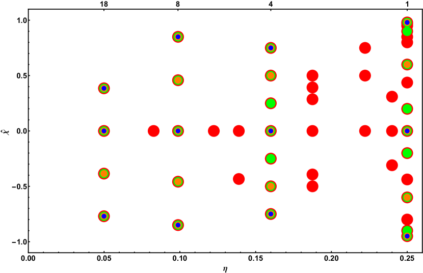
The construction of previous phenomenological models Ajith et al. (2007, 2008, 2011); Santamaría et al. (2010) suggested that the parameter dependence of the coefficients in our models depend sufficiently smoothly across the parameter space that each coefficient can be presented by a low-order polynomial in each parameter, and therefore we require only 4-5 waveforms for each direction in parameter space. This expectation is borne out in the current model, where we use four values of the mass ratio (1, 4, 8 and 18) and four or five values of the spin at each mass ratio.

In this section we consider versions of the model constructed with more (or less) calibration waveforms. We find that our small set of 19 calibration waveforms is just as accurate as a model that is calibrated against a much larger set of 48 waveforms. To quantify this test we compute the maximum mismatch of four distinct models against all hybrid waveforms used in this paper, i.e., the 48 waveforms in Tabs. 1 and 3.

Fig 17 indicates four choices of parameter-space coverage. The first set is the largest, and includes all 48 configurations indicated in the figure. The second set includes 25 waveforms, but only at mass ratios 1, 4 8 and 18, and does not include all available spin values at mass ratios 1 and 8. The third set consists of the 19 waveforms that we use for our final model. The fourth set is more sparsely sampled in spins, with only three spin values at each mass ratio, and only 12 waveforms in total.

Four models were constructed, each using the same prescription, except for the Set-4 model, for which we used a lower-order fit in the $\hat{\chi}$ direction, since in general we cannot expect to fit four coefficients with only three spin values.

The results are summarized in Tab. 4. We calculate the mismatch between each of the models and all 48 hybrids, over the same mass range used in Sec. IX.1 using the early aLIGO noise curve with a 30 Hz cut off. For each hybrid we calculate the largest mismatch in that mass range. The table indicates the number of configurations for which we find mismatches larger than 0.1%, 1% and 3% for each model. As we have already seen in Fig. 15, the fiducial Set-3 model has mismatches of less than 1% for all configurations. We find that increasing the number of calibration waveforms does not significantly improve the model’s performance.

We also see that if we further reduce the number of calibration waveforms, as in the Set-4 model, then the accuracy of the model drops significantly. For this model there are now three configuration with mismatches worse than 1%, and one configuration with a mismatch worse than 7%. We therefore conclude that, in the sense of the simple comparison that has been performed here, the Set-3 model represents the optimal choice of calibration waveforms.

Figure 17: Four sets of calibration waveforms. Set 1 (48 waveforms) is indicated in red, Set 2 (25 waveforms) in green, Set 3 (19 waveforms, used for the final PhenomD model) in orange, and Set 4 (12 waveforms) in blue.

Model	# waveforms	$>0.1$%	$>1$%	$>3$%	$\max\mathcal{M}$ (%)
Set 1	48	19	0	0	0.94
Set 2	25	27	0	0	0.83
Set 3 (*)	19	29	0	0	0.87
Set 4	12	37	3	1	7.82

Table 4: Comparison of models constructed with different sets of calibration waveforms. The table shows, for each calibration set (see Fig. 17), the number of verifications waveforms (out of 48) for which there is a mismatch $\mathcal{M}$ above $0.1$%, 1%, or 3%, over the same mass range used in Sec. IX.1 using the early aLIGO noise curve with a 30 Hz cut off. We see that with a small set of 19 waveforms we achieve comparable mismatches to models which used larger sets of calibration waveforms, and that using less waveforms significantly degrades the quality of the model. Set 3 is used for the final model.

X Model vs Model Comparisons

We have demonstrated the high degree of fidelity of PhenomD to both the waveforms that were used in calibrating the model and to those that were not. Without further comparisons to NR waveforms we cannot rigorously quantify the accuracy of our, or indeed any, waveform model. However, it is reasonable to assume that if two independent waveform models agree over a portion of the parameter space then we can gain some well-founded confidence in their accuracy.

The computational cost of the SEOBNRv2 model makes it difficult to make detailed comparisons across the entire parameter space with high resolution in $(\eta,\hat{\chi})$. However, based upon the recent work in Ref. Pürrer (2014), a reduced order model (ROM) of SEOBNRv2, called SEOBNRv2_ROM, has been developed Pürrer (in prep.). This is a fast, frequency-domain approximation to the SEOBNRv2 model that has a worst mismatch against SEOBNRv2 of $1\%$, but in general mismatches are better than $\sim 0.1\%$. SEOBNRv2_ROM is a two spin model which can be used to estimate SEOBNRv2 waveforms with symmetric mass-ratios $\eta\in[0.01,0.25]$ and spins $\chi_{i}\in[-1,0.99]$. The ROM can be used over the frequency range $Mf\in[0.0001,0.3]$ Note that the underlying SEOBNRv2 model was calibrated to NR waveforms up to mass-ratios 1:8 and spins up to 0.5 (except along the equal mass line where spins in the range $[-0.95,0.98]$ were used). The merger-ringdown parts of the PhenomD and SEOBNRv2 models are almost completely independent of one another with the only common features being that they share some of the same calibration waveforms, i.e., the ones from the public SXS catalogue and also the same underlying EOB Hamiltonian.

During the following comparison we restrict the computation of the mismatch to the frequencies of the SEOBNRv2_ROM, namely $[0.0006,0.135]$, using the design sensitivity noise curve with a lower frequency cut-off of 10 Hz as in previous sections.

Figure 18: Mismatch comparisons between the SEOBNRv2_ROM model, and three versions of PhenomD. Left: the final PhenomD model. Middle: SEOBNRv2_ROM is used for the inspiral part of PhenomD, i.e., up to $Mf=0.018$. Right: TaylorF2 is used for the inspiral part of PhenomD. See text for discussion.

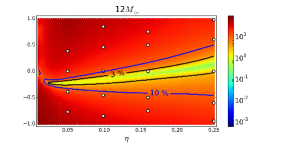
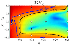
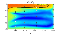
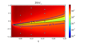
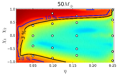
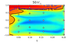
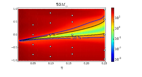
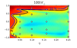
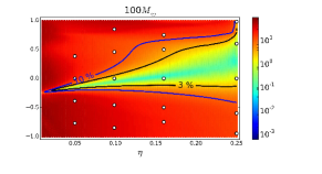
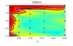
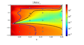
We noted earlier that the PhenomD model is modular, and we can use alternative models of either the inspiral or merger-ringdown regions as we wish. In the following comparisons we consider three versions of the model. One is the full PhenomD model that we have presented in the previous sections. In comparisons with SEOBNRv2_ROM at low masses, the mismatch is dominated by differences between the uncalibrated SEOBv2 model that we used to calibrate the inspiral of PhenomD, and the calibrated SEOBNRv2 model; it is a reflection of a different choice of inspiral approximant, and not the inherent accuracy of either model. For this reason we also perform a second set of comparisons, where we use SEOBNRv2_ROM for the inspiral (Region I) part of PhenomD; the merger-ringdown (Region II) remains unchanged. This allows us to compare PhenomD and SEOBNRv2_ROM over only the merger-ringdown, and also illustrates the flexibility of the PhenomD model in using alternative inspiral approximants. Finally, we replace the inspiral part of the PhenomD with TaylorF2.

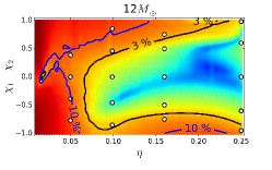
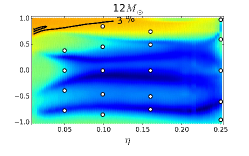
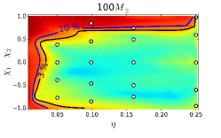
The results of our comparions are shown in Fig. 18. Each panel shows the mismatch in percentage between the PhenomD model and SEOBNRv2_ROM (left column) and between [SEOBNRv2_ROM-inspiral + PhenomD-merger-ringdown] and SEOBNRv2_ROM (middle column), and between [TaylorF2-inspiral + PhenomD-merger-ringdown] and SEOBNRv2_ROM (right column). The calculations were performed over mass ratios $[1,100]$, spins in the range $[-1,0.99]$ and for the total masses $[12,20,50,100,150]M_{\odot}$. Overlaid in white dots are the calibration points of the PhenomD model. It is instructive when studying these plots to recall that the common region of parameter space calibration is up to mass-ratios 1:8 ($\eta\sim 0.01$) and spin $[-0.5,0.5]$, except along the equal mass line where the spins range from $[-0.95,0.98]$.

We focus first on the low-mass configurations ($M<50\,M_{\odot}$). We see that the agreement between PhenomD and SEOBNRv2_ROM is in general quite poor — some parts of the common calibration region of both models show mismatches greater than 3%, e.g, for anti-aligned spins. This is not necessarily due to the innaccuracy of either model. We have seen in Fig. 15 that PhenomD typically has matches of better than 1% against our hybrid waveforms, which demonstrates that the model accurately reproduces the uncalibrated SEOBv2 model at low frequencies. Therefore, we expect that the poor mismatches between PhenomD and SEOBNRv2_ROM at low masses are due to differences between SEOBv2 and the calibrated SEOBNRv2 inspiral. This expectation is borne out in the middle column, where the SEOBv2-based PhenomD inspiral is replaced with the SEOBNRv2_ROM inspiral. Now the modified PhenomD and SEOBNRv2_ROM models differ only in their description of the merger-ringdown, and should agree well at very low masses, where the merger-ringdown contributes little signal-to-noise ratio (SNR). This is what we find: at $12\,M_{\odot}$ the mismatches are better than 1% for most of the parameter space. The merger-ringdown still has some influence, increasing the mismatches for high-spin and high-mass-ratio systems, but in general the agreement is extremely good.

Although the uncalibrated SEOBv2 and the calibrated SEOBNRv2 inspirals show poor matches at low masses, we note that both are still consistent with our full NR data at higher frequencies, and both are adequate options for an inspiral description, as we discussed in detail in Paper 1, and also in Sec. IV above. The right panel illustrates how the model would change if we instead used TaylorF2 for the inspiral. At the matching frequency with the merger-ringdown model ($Mf=0.018$) the TaylorF2 phase disagree (in the sense of the time-shift analysis in Paper 1) at a level that makes it difficult to smoothly connect them over large regions of the parameter space. This, in addition to the differences between TaylorF2 and SEOBv2(NR) at low frequencies, introduces high overlaps over all but a small strip of parameter space.

As we progress down the table of plots to higher masses, the merger-ringdown contributes more power to the SNR, and the results of the left and middle comparisons agree more. At $150\,M_{\odot}$, where the contribution from the inspiral (taken here as $Mf<0.018$) is negligible, we see that the two comparisons are almost identical. The poor agreement between TaylorF2 and our merger-ringdown model at $Mf=0.018$ continues to lead to large mismatches.

We now focus on the high-mass configurations ($M\geq 50\,M_{\odot}$), and the left panels that directly compare PhenomD and SEOBNRv2_ROM. It is evident that the region of agreement between the two models follows closely the region of common calibration points. Indeed, it is very encouraging that there is a high level of agreement between these two independent models even up to high mass-ratios of 1:18 and towards large negative spin values.

The positive spin section shows a different behaviour. At high masses (i.e., where the merger and ringdown are in the detector’s most sensitive frequency range), there is a sudden drop in the agreement between the two models at mass-ratios larger than equal mass and spin greater than $\sim 0.75$.

PhenomD is calibrated to two high-spin unequal-mass cases, $(q,\chi_{1},\chi_{2})=\{(4,0.75,0.75),(8,0.85,0.85)\}$, and we have one additional case for verification, $(2,0.75,0.75)$. These are the waveforms A10 and A15 from Table 1 and B17 from Table 3 respectively. As we have already seen, PhenomD has better than 1% mismatch to all theses cases and therefore the poor mismatches are unlikely due to errors in PhenomD. We note that these cases are well outside the calibration region of the SEOBNRv2 model, and we therefore suspect that the accuracy of its description of the merger-ringdown degrades significantly for high spins.

Our results also suggest that, despite the lack of calibration waveforms at high anti-aligned spins, the SEOBNRv2 model remains accurate in that region of parameter space, and the relatively good agreement between the two models even for nearly extreme anti-aligned spins suggests that additional calibration waveforms, while they would be valuable, are less crucial in those cases.

We also observe poor mismatches for very high mass ratios. However, since this is outside the calibration region of both models, we cannot conclude which (if either) is correct.

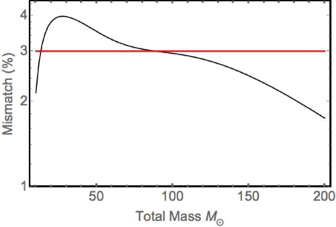
To illustrate further the disagreement between PhenomD and SEOBNRv2 at unequal masses and high spins, we consider in more detail the three NR configurations that we have available. Fig. 19 shows mismatches between pure NR waveforms (not the hybrids) for each of these cases, and against the PhenomD and SEOBNRv2 models, using the techniques discussed in Sec. II.2. The mismatch against SEOBNRv2 is above 1% for all masses, and can be as high as 10%. We have reproduced these plots using SEOBNRv2 waveforms generated from the LAL code, and the results are indistinguishable; the poor mismatches cannot be attributed to any errors in the ROM construction.

We therefore conclude that the merger and ringdown are not accurately represented in the SEOBNRv2 model for high spins. This does not detract from the power of the EOB NR approach, but simply illustrates that we should not expect any merger-ringdown model to be accurate outside its region of NR calibration. The same applies to our PhenomD model; we cannot make any statements on its accuracy for spins with $\hat{\chi}\gtrsim 0.85$, other than for equal-mass systems.

Figure 19: Mismatch of PhenomD (solid) or SEOBNRv2_ROM (dashed) against cases A10 (orange), A15 (green) and B17 (black).

XI Summary and discussion

We have presented a new phenomenological model of the GW signal from the inspiral, merger and ringdown of aligned-spin BH binaries, PhenomD. The new model is calibrated to hybrid EOB+NR waveforms that cover the largest region of parameter space of any aligned-spin model to date — mass ratios up to 1:18 and spins up to $a/m\sim 0.85$. The inspiral and merger-ringdown are described by three separate models, allowing high accuracy over the full frequency range detectable by aLIGO and AdV, and also making the model modular: the inspiral and merger-ringdown parts can easily be modified or replaced if improved or extended models (e.g., to a yet larger region of parameter space) become available.

The inspiral part of our hybrids consists of uncalibrated SEOBv2 waveforms. We have shown in Paper 1 that the SEOBv2 waveforms are the most consistent with our NR simulations over the full parameter space that we consider, and we choose to use uncalibrated SEOBv2 to produce a model that is fully independent of the NR calibration done to produce SEOBNRv2.

The merger-ringdown part of the hybrids (i.e., the NR waveforms) have a common lowest frequency of $Mf\sim 0.018$, and so this is the frequency at which we switch from the inspiral to the merger-ringdown model.

The final model has mismatches against both the 19 calibration hybrids and an additional 29 verification hybrids, of typically better than 1% for all masses. The mismatches are shown in Fig. 15, and demonstrate that we have faithfully modelled this region of the aligned-spin parameter space.

The model is parameterized by the binary’s symmetric mass ratio, $\eta$, and a normalized reduced effective spin parameter, $\hat{\chi}$, defined in Eq. (4). A parameterization in terms of a weighted sum of the two BH spins has been used in previous Phenom models Ajith et al. (2011); Santamaría et al. (2010), and is motivated by the leading-order spin effect on the inspiral phasing Cutler and Flanagan (1994); Poisson and Will (1995); Ajith (2011), and demonstrations of its efficacy for merger-ringdown Pürrer et al. (2013). In this paper we show that the reduced-spin approximation becomes inaccurate only for high-spin unequal-mass systems, but in these configurations the parameter errors due to our approximation appear to be smaller than statistical errors in the spin and mass-ratio measurements with aLIGO and AdV. This implies that it will be difficult to measure both BH spins in GW measurements; this will be considered in more detail in a forthcoming paper Pürrer et al. (in prep.).

We have compared the new PhenomD model with the state-of-the-art SEOBNRv2 model, and found that the two models agree well over their common region of calibration, which is mass ratios up to 1:8, and spins up to $a/m\sim 0.5$ (and near-extremal spins for equal-mass systems). At low masses the agreement is not good, but we show that this is due to differences between the calibrated and uncalibrated SEOBv2 inspiral descriptions.

Outside the common calibration region, the two models show significant disagreement, in terms of their mismatch. This is particularly true for high aligned spins. Given that PhenomD was calibrated to several high-spin unequal-mass simulations (spins of 0.75 or 0.85), while SEOBNRv2 was calibrated to spins of no higher than 0.5 for unequal-mass configurations, we conclude that SEOBNRv2 does not accurately capture the merger and ringdown for these systems. We expect, however, that its performance will become comparable to PhenomD when calibrated to additional NR waveforms.

The broader conclusion we draw from these results is that high-aligned-spin systems deserve greater attention in future modelling efforts. The PhenomD model was calibrated to only two high-aligned-spin binaries, but it is clear that a larger number of NR simulations in this region of parameter space will benefit GW astronomy.

The PhenomD model involves 17 coefficients that are mapped across the parameter space with polynomials up to second order in $\eta$ and up to third order in $\hat{\chi}$. Although the total number of coefficients is similar to the previous PhenomC model, the development of a refined ansatz for each frequency region allows us to more accurately model a wider range of features of the waveforms. This is described in more detail in Paper 1. We have also carefully tuned each ansatz, and our parameter-space fits, to ensure that the model produces physically reasonable results outside the calibration region, and that the waveforms show no pathological features when converted to the time-domain (Appendix A). These modifications significantly improve the model beyond previous Phemom models, in addition to increasing the range of calibration and lowering the mismatch error.

In previous work we have shown that models for generic (precessing) binaries can be produced by “twisting up” an aligned-spin model. The PhenomP model exploits that idea, but to date has been based on the PhenomC model, which limits its applicability to mass ratios $q\lesssim 4$. With the advent of PhenomD, we will be able to make PhenomP valid to much higher mass ratios and higher values of the parallel component of the spin. This simple replacement of PhenomC with PhenomD in the LIGO-Virgo LAL code has already been tested, and will be made available in the near future.

Appendix A Time-domain conversion

Our PhenomD model is formulated entirely in the frequency domain, which is a great advantage for performing fast GW searches and parameter estimation studies. However, our construction process started with data in the time domain, and physical signals are smooth functions in both the frequency and time domain. Therefore, it is desirable to check how our model transforms from the frequency domain back into the time domain via a straightforward inverse Fourier transformation.

This serves also as an independent, powerful sanity check. The previous PhenomC model Santamaría et al. (2010), for instance, quickly develops a pathological behavior in the time domain once the parameters leave the calibration region, which is a result of steep transitions caused by extrapolating fitting coefficients. We do not find these features for our new PhenomD model.

Before applying the inverse Fourier transformation, we multiply our model with a variant of the Planck taper function McKechan et al. (2010),

$$\mathcal{T}(f)=\begin{cases}0,&f\leq f_{1}\\ \left[\exp\left(\frac{f_{2}-f_{1}}{f-f_{1}}+\frac{f_{2}-f_{1}}{f-f_{2}}\right)+1\right]^{-1},&f_{1}<f<f_{2}\\ 1,&f>f_{2}\end{cases},$$

where $f_{2}$ is the smallest frequency that we want to represent in the time-domain data (which become infinitively long for $f_{2}\to 0$). In order to avoid a sharp transition, which would introduce unphysical oscillations, $\mathcal{T}$ uses an extra cushion, $f\in(f_{1},f_{2})$, in which the frequency domain amplitude smoothly increases from zero to their correct value. We typically set $f_{1}=0.8f_{2}$.

We perform the Fourier transformation numerically, which requires us to define a suitable sampling rate in the time and frequency domain. From our model, we find that the amplitude has dropped several orders of magnitude for frequencies $Mf>0.25$, so we can choose any sampling with $\Delta t/M<2$ which in turn is solely determined by the largest frequency we include in our frequency-domain data.

The frequency-domain sampling, on the other hand, is determined by the total length of the signal in the time domain, which is information we do not have a priori access to. However, in the spirit of the stationary-phase approximation that typically relates the time-domain phase derivative to the frequency ($d\phi(t)/dt\approx 2\pi f$), we approximate

$$\frac{d\phi(f)}{df} =\phi^{\prime}(f)\approx 2\pi t,$$ (39)

$$\Rightarrow~{}~{}\Delta f <\frac{1}{t_{\rm max}-t_{1}}\approx\frac{\pi}{|\phi^{\prime}(f_{\rm max})-\phi^{\prime}(f_{1})|}.$$ (40)

In (40), we have introduced an extra factor of $1/2$ to account for the negative-frequency content of real-valued signals (just like in the usual sampling theorem), and when choosing $\Delta f$ we usually apply another factor of $1/2$ as safety margin.

\begin{overpic}[height=99.58464pt]{q1_98TD} \put(11.0,24.0){$q=1,~{}\chi_{1}=\chi_{2}=0.98$} \end{overpic}

\begin{overpic}[height=99.58464pt]{q1_m95TD} \put(11.0,24.0){$q=1,~{}\chi_{1}=\chi_{2}=-0.95$} \end{overpic}

\begin{overpic}[height=99.58464pt]{q8_85TD} \put(11.0,24.0){$q=8,~{}\chi_{1}=\chi_{2}=0.85$} \end{overpic}

\begin{overpic}[height=99.58464pt]{q8_m85TD} \put(11.0,24.0){$q=8,~{}\chi_{1}=\chi_{2}=-0.85$} \end{overpic}

\begin{overpic}[height=99.58464pt]{q18_4TD} \put(11.0,24.0){$q=18,~{}\chi_{1}=0.4,~{}\chi_{2}=0.$} \end{overpic}

\begin{overpic}[height=99.58464pt]{q18_m8TD} \put(11.0,24.0){$q=18,~{}\chi_{1}=-0.8,~{}\chi_{2}=0.$} \end{overpic}

Figure 20: Time-domain PhenomD waveforms (solid, light blue online) and NR waveforms (dashed, red online) for corners of the parameter space used for calibration. We plot the plus polarization $h_{+}$ normalized by the extraction radius, and the binary’s parameters are indicated by the mass ratio $q=m_{1}/m_{2}$ and the two spin parameters $\chi_{1},\chi_{2}$.

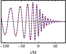
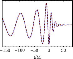
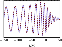
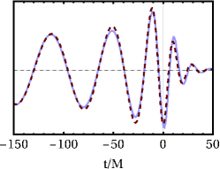
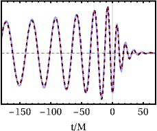
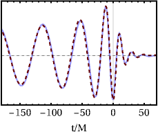
The time-domain waveforms we obtain this way can be compared to the original NR data, and for corners of the parameter space used for calibration we show the results in Fig. 20. Note that a small overall time and phase shift was applied to the model, as these parameters are not meant to faithfully capture the arbitrary choices made in the original NR simulations. No other optimization has been applied. The agreement visible in Fig. 20 throughout the late inspiral, merger and ringdown is remarkable and a strong indication (in additional to the matches presented in Sec. IX.1) that our hybridization, fitting and interpolation procedures accurately represent the original data.

Figure 21: Time-domain representation of the PhenomD model outside its calibration region, here for mass ratio 50 and spin parameters of $\chi_{1}=\chi_{2}=0.99$.

In addition to complementing the model validation, we may also use the time-domain representations as a visual sanity check, even outside the model’s calibration region. As mentioned above, this proved to be a powerful test of the previous PhenomC model that failed to produce reasonable time-domain waveforms in many parts of the parameter space outside its calibration range. PhenomD, however, does not show any pathological behavior outside its calibration region, neither in the time nor frequency domain. We illustrate this fact in Fig. 21 by showing a case where the model parameters have been extrapolated to mass ratio 50 and near-extremal spins $\chi_{1}=\chi_{2}=0.99$. While such a plot is by no means a guarantee that the waveforms are accurate in this regions of the parameter space, it is reassuring that our new model is much more robust in its extrapolation, which will allow GW search algorithms to use our model slightly outside its calibration region, even if we cannot vouch for the level of accuracy there.

Appendix B PN coefficients

For the convenience of the reader, we list below the PN coefficients implemented in our model. We incorporated spin-independent corrections up to 3.5PN order ($i=7$) Buonanno et al. (2009b); Blanchet (2014), linear spin-orbit corrections up to 3.5PN order Bohé et al. (2013) and quadratic spin corrections up to 2PN order Poisson (1998); Arun et al. (2009); Mikoczi et al. (2005). Our re-expansion strategy follows the choices made in the current state of the LIGO software library The LIGO Scientific Collaboration (2015) as discussed in Sec. VI.1.

Following (27), we express the frequency-domain phase as

$$\begin{split}\phi_{\text{TF2}}&=\,2\pi ft_{c}-\varphi_{c}-\pi/4\\ &+\frac{3}{128\,\eta}(\pi fM)^{-5/3}\sum_{i=0}^{7}\varphi_{i}(\Xi)(\pi fM)^{i/3}.\end{split}$$

The individual masses and spin parameters, $m_{i}$ and $\chi_{i}$ ($i=1,2$), are encoded in the following parameter combinations,

$$M =m_{1}+m_{2},$$ (41)

$$\eta =m_{1}\,m_{2}/M^{2},$$ (42)

$$\delta =(m_{1}-m_{2})/M,$$ (43)

$$\chi_{s} =(\chi_{1}+\chi_{2})/2,$$ (44)

$$\chi_{a} =(\chi_{1}-\chi_{2})/2.$$ (45)

The expansion coefficients are then given by

$$\varphi_{0} =1,$$ (46)

$$\varphi_{1} =0,$$ (47)

$$\varphi_{2} =\frac{3715}{756}+\frac{55\eta}{9},$$ (48)

$$\varphi_{3} =-16\pi+\frac{113\delta\chi_{a}}{3}+\left(\frac{113}{3}-\frac{76\eta}{3}\right)\chi_{s},$$ (49)

$$\varphi_{4} =\frac{15293365}{508032}+\frac{27145\eta}{504}+\frac{3085\eta^{2}}{72}+\left(-\frac{405}{8}+200\eta\right)\chi_{a}^{2}-\frac{405}{4}\delta\chi_{a}\chi_{s}+\left(-\frac{405}{8}+\frac{5\eta}{2}\right)\chi_{s}^{2},$$ (50)

$$\varphi_{5} =\left[1+\log\left(\pi Mf\right)\right]\left[\frac{38645\pi}{756}-\frac{65\pi\eta}{9}+\delta\left(-\frac{732985}{2268}-\frac{140\eta}{9}\right)\chi_{a}+\left(-\frac{732985}{2268}+\frac{24260\eta}{81}+\frac{340\eta^{2}}{9}\right)\chi_{s}\right],$$ (51)

$$\begin{split}\varphi_{6}&=\frac{11583231236531}{4694215680}-\frac{6848\gamma_{E}}{21}-\frac{640\pi^{2}}{3}+\left(-\frac{15737765635}{3048192}+\frac{2255\pi^{2}}{12}\right)\eta+\frac{76055\eta^{2}}{1728}-\frac{127825\eta^{3}}{1296}\\ &\phantom{=}-\frac{6848}{63}\log(64\pi Mf)+\frac{2270}{3}\pi\delta\chi_{a}+\left(\frac{2270\pi}{3}-520\pi\eta\right)\chi_{s},\end{split}$$ (52)

$$\begin{split}\varphi_{7}&=\frac{77096675\pi}{254016}+\frac{378515\pi\eta}{1512}-\frac{74045\pi\eta^{2}}{756}+\delta\left(-\frac{25150083775}{3048192}+\frac{26804935\eta}{6048}-\frac{1985\eta^{2}}{48}\right)\chi_{a}\\ &\phantom{=}+\left(-\frac{25150083775}{3048192}+\frac{10566655595\eta}{762048}-\frac{1042165\eta^{2}}{3024}+\frac{5345\eta^{3}}{36}\right)\chi_{s}.\end{split}$$ (53)

As discussed in Sec. VI.2 and Sec. IV in Paper 1, our inspiral amplitude model is based on a re-expanded PN amplitude. The expansion coefficients of Eq. (29) are given by

$$\mathcal{A}_{0} =1,$$ (54)

$$\mathcal{A}_{1} =0,$$ (55)

$$\mathcal{A}_{2} =-\frac{323}{224}+\frac{451\eta}{168},$$ (56)

$$\mathcal{A}_{3} =\frac{27\delta\chi_{a}}{8}+\left(\frac{27}{8}-\frac{11\eta}{6}\right)\chi_{s},$$ (57)

$$\mathcal{A}_{4} =-\frac{27312085}{8128512}-\frac{1975055\eta}{338688}+\frac{105271\eta^{2}}{24192}+\left(-\frac{81}{32}+8\eta\right)\chi_{a}^{2}-\frac{81}{16}\delta\chi_{a}\chi_{s}+\left(-\frac{81}{32}+\frac{17\eta}{8}\right)\chi_{s}^{2},$$ (58)

$$\begin{split}\mathcal{A}_{5}&=-\frac{85\pi}{64}+\frac{85\pi\eta}{16}+\delta\left(\frac{285197}{16128}-\frac{1579\eta}{4032}\right)\chi_{a}+\left(\frac{285197}{16128}-\frac{15317\eta}{672}-\frac{2227\eta^{2}}{1008}\right)\chi_{s},\end{split}$$ (59)

$$\begin{split}\mathcal{A}_{6}&=-\frac{177520268561}{8583708672}+\left(\frac{545384828789}{5007163392}-\frac{205\pi^{2}}{48}\right)\eta-\frac{3248849057\eta^{2}}{178827264}+\frac{34473079\eta^{3}}{6386688}\\ &+\left(\frac{1614569}{64512}-\frac{1873643\eta}{16128}+\frac{2167\eta^{2}}{42}\right)\chi_{a}^{2}+\left(\frac{31\pi}{12}-\frac{7\pi\eta}{3}\right)\chi_{s}+\left(\frac{1614569}{64512}-\frac{61391\eta}{1344}+\frac{57451\eta^{2}}{4032}\right)\chi_{s}^{2}\\ &+\delta\chi_{a}\left(\frac{31\pi}{12}+\left(\frac{1614569}{32256}-\frac{165961\eta}{2688}\right)\chi_{s}\right)\end{split}$$ (60)

Appendix C Phenomenological Coefficients

The values of the coefficients for the mapping functions given in Eq. (31) are shown in Tab. 5. These values are calculated under the parametrization ($\eta$, $\chi_{\rm{PN}}$).

$\Lambda^{i}$	$\lambda_{00}$	$\lambda_{10}$	$\lambda_{01}$	$\lambda_{11}$	$\lambda_{21}$	$\lambda_{02}$	$\lambda_{12}$	$\lambda_{22}$	$\lambda_{03}$	$\lambda_{13}$	$\lambda_{23}$
$\rho_{1}$	3931.9	-17395.8	3132.38	343966.	-1.21626$\times 10^{6}$	-70698.	1.38391$\times 10^{6}$	-3.96628$\times 10^{6}$	-60017.5	803515.	-2.09171$\times 10^{6}$
$\rho_{2}$	-40105.5	112253.	23561.7	-3.47618$\times 10^{6}$	1.13759$\times 10^{7}$	754313.	-1.30848$\times 10^{7}$	3.64446$\times 10^{7}$	596227.	-7.42779$\times 10^{6}$	1.8929$\times 10^{7}$
$\rho_{3}$	83208.4	-191238.	-210916.	8.71798$\times 10^{6}$	-2.69149$\times 10^{7}$	-1.98898$\times 10^{6}$	3.0888$\times 10^{7}$	-8.39087$\times 10^{7}$	-1.4535$\times 10^{6}$	1.70635$\times 10^{7}$	-4.27487$\times 10^{7}$
$v_{2}$	0.814984	2.57476	1.16102	-2.36278	6.77104	0.757078	-2.72569	7.11404	0.176693	-0.797869	2.11624
$\gamma_{1}$	0.0069274	0.0302047	0.00630802	-0.120741	0.262716	0.00341518	-0.107793	0.27099	0.000737419	-0.0274962	0.0733151
$\gamma_{2}$	1.01034	0.000899312	0.283949	-4.04975	13.2078	0.103963	-7.02506	24.7849	0.030932	-2.6924	9.60937
$\gamma_{3}$	1.30816	-0.00553773	-0.0678292	-0.668983	3.40315	-0.0529658	-0.992379	4.82068	-0.00613414	-0.384293	1.75618
$\sigma_{1}$	2096.55	1463.75	1312.55	18307.3	-43534.1	-833.289	32047.3	-108609.	452.251	8353.44	-44531.3
$\sigma_{2}$	-10114.1	-44631.	-6541.31	-266959.	686328.	3405.64	-437508.	1.63182$\times 10^{6}$	-7462.65	-114585.	674402.
$\sigma_{3}$	22933.7	230960.	14961.1	1.19402$\times 10^{6}$	-3.10422$\times 10^{6}$	-3038.17	1.87203$\times 10^{6}$	-7.30915$\times 10^{6}$	42738.2	467502.	-3.06485$\times 10^{6}$
$\sigma_{4}$	-14621.7	-377813.	-9608.68	-1.71089$\times 10^{6}$	4.33292$\times 10^{6}$	-22366.7	-2.50197$\times 10^{6}$	1.02745$\times 10^{7}$	-85360.3	-570025.	4.39684$\times 10^{6}$
$\beta_{1}$	97.8975	-42.6597	153.484	-1417.06	2752.86	138.741	-1433.66	2857.74	41.0251	-423.681	850.359
$\beta_{2}$	-3.2827	-9.05138	-12.4154	55.4716	-106.051	-11.953	76.807	-155.332	-3.41293	25.5724	-54.408
$\beta_{3}$	-2.51564$\times 10^{-5}$	1.97503$\times 10^{-5}$	-1.83707$\times 10^{-5}$	2.18863$\times 10^{-5}$	8.25024$\times 10^{-5}$	7.15737$\times 10^{-6}$	-5.578$\times 10^{-5}$	1.91421$\times 10^{-4}$	5.44717$\times 10^{-6}$	-3.22061$\times 10^{-5}$	7.97402$\times 10^{-5}$
$\alpha_{1}$	43.3151	638.633	-32.8577	2415.89	-5766.88	-61.8546	2953.97	-8986.29	-21.5714	981.216	-3239.57
$\alpha_{2}$	-0.0702021	-0.162698	-0.187251	1.13831	-2.83342	-0.17138	1.71975	-4.53972	-0.0499834	0.606207	-1.68277
$\alpha_{3}$	9.59881	-397.054	16.2021	-1574.83	3600.34	27.0924	-1786.48	5152.92	11.1757	-577.8	1808.73
$\alpha_{4}$	-0.0298949	1.40221	-0.0735605	0.833701	0.224001	-0.0552029	0.566719	0.718693	-0.0155074	0.157503	0.210768
$\alpha_{5}$	0.997441	-0.00788445	-0.0590469	1.39587	-4.51663	-0.0558534	1.75166	-5.99021	-0.0179453	0.59651	-2.06089

Table 5: Coefficient values for the mapping functions given in Eq. (31). These values are calculated under the parametrisation ($\eta$, $\chi_{\rm{PN}}$)

References

- Abbott et al. (2009) B. Abbott et al. (LIGO Scientific Collaboration), Rept.Prog.Phys. 72, 076901 (2009), eprint 0711.3041.
- Harry and LIGO Scientific Collaboration (2010) G. M. Harry and LIGO Scientific Collaboration, Classical and Quantum Gravity 27, 084006 (2010).
- Shoemaker and the Advanced LIGO Team (2009) D. Shoemaker and the Advanced LIGO Team, LIGO-M060056 (2009).
- Accadia et al. (2011) T. Accadia, F. Acernese, F. Antonucci, P. Astone, G. Ballardin, et al., Class.Quant.Grav. 28, 114002 (2011).
- Aasi et al. (2013a) J. Aasi et al. (LIGO Scientific Collaboration, Virgo Collaboration) (2013a), eprint 1304.0670.
- Sathyaprakash and Schutz (2009) B. S. Sathyaprakash and B. F. Schutz, Living Rev. Rel. 12, 2 (2009), eprint 0903.0338.
- Hannam (2014) M. Hannam, Gen. Rel. Grav. 46, 1767 (2014), eprint 1312.3641.
- Ajith et al. (2011) P. Ajith, M. Hannam, S. Husa, Y. Chen, B. Brügmann, N. Dorband, D. Müller, F. Ohme, D. Pollney, C. Reisswig, et al., Physical Review Letters 106 (2011), ISSN 1079-7114, URL http://dx.doi.org/10.1103/PhysRevLett.106.241101.
- Harry et al. (2014) I. Harry, A. Nitz, D. A. Brown, A. Lundgren, E. Ochsner, et al., Phys.Rev. D89, 024010 (2014), eprint 1307.3562.
- Dal Canton et al. (2015) T. Dal Canton, A. P. Lundgren, and A. B. Nielsen, Phys. Rev. D91, 062010 (2015), eprint 1411.6815.
- Schmidt et al. (2012) P. Schmidt, M. Hannam, and S. Husa, Phys. Rev. D86, 104063 (2012), eprint 1207.3088.
- Ajith et al. (2007) P. Ajith, S. Babak, Y. Chen, M. Hewitson, B. Krishnan, J. T. Whelan, B. Brügmann, P. Diener, J. Gonzalez, M. Hannam, et al., Class. Quantum Grav. 24, S689 (2007), ISSN 1361-6382, URL http://dx.doi.org/10.1088/0264-9381/24/19/S31.
- Ajith et al. (2008) P. Ajith et al., Phys. Rev. D77, 104017 (2008), [Erratum: Phys. Rev.D79,129901(2009)], eprint 0710.2335.
- Santamaría et al. (2010) L. Santamaría, F. Ohme, P. Ajith, B. Brügmann, N. Dorband, M. Hannam, S. Husa, P. Mösta, D. Pollney, C. Reisswig, et al., Phys. Rev. D 82 (2010), ISSN 1550-2368, URL http://dx.doi.org/10.1103/PhysRevD.82.064016.
- Buonanno et al. (2007) A. Buonanno, Y. Pan, J. G. Baker, J. Centrella, B. J. Kelly, S. T. McWilliams, and J. R. van Meter, Phys. Rev. D76, 104049 (2007), eprint 0706.3732.
- Buonanno et al. (2009a) A. Buonanno, Y. Pan, H. P. Pfeiffer, M. A. Scheel, L. T. Buchman, and L. E. Kidder, Phys. Rev. D79, 124028 (2009a), eprint 0902.0790.
- Damour et al. (2008a) T. Damour, A. Nagar, E. N. Dorband, D. Pollney, and L. Rezzolla, Phys. Rev. D77, 084017 (2008a), eprint 0712.3003.
- Damour et al. (2008b) T. Damour, A. Nagar, M. Hannam, S. Husa, and B. Bruegmann, Phys. Rev. D78, 044039 (2008b), eprint 0803.3162.
- Damour and Nagar (2009) T. Damour and A. Nagar, Phys. Rev. D79, 081503 (2009), eprint 0902.0136.
- Pan et al. (2010) Y. Pan, A. Buonanno, L. T. Buchman, T. Chu, L. E. Kidder, H. P. Pfeiffer, and M. A. Scheel, Phys. Rev. D81, 084041 (2010), eprint 0912.3466.
- Yunes et al. (2010) N. Yunes, A. Buonanno, S. A. Hughes, M. Coleman Miller, and Y. Pan, Phys. Rev. Lett. 104, 091102 (2010), eprint 0909.4263.
- Pan et al. (2011) Y. Pan, A. Buonanno, M. Boyle, L. T. Buchman, L. E. Kidder, H. P. Pfeiffer, and M. A. Scheel, Phys. Rev. D84, 124052 (2011), eprint 1106.1021.
- Taracchini et al. (2012) A. Taracchini, Y. Pan, A. Buonanno, E. Barausse, M. Boyle, T. Chu, G. Lovelace, H. P. Pfeiffer, and M. A. Scheel, Phys. Rev. D86, 024011 (2012), eprint 1202.0790.
- Damour et al. (2013) T. Damour, A. Nagar, and S. Bernuzzi, Phys.Rev. D87, 084035 (2013), eprint 1212.4357.
- Pan et al. (2014) Y. Pan, A. Buonanno, A. Taracchini, L. E. Kidder, A. H. Mroué, H. P. Pfeiffer, M. A. Scheel, and B. Szilágyi, Phys. Rev. D 89 (2014), ISSN 1550-2368, URL http://dx.doi.org/10.1103/PhysRevD.89.084006.
- Taracchini et al. (2014a) A. Taracchini, A. Buonanno, Y. Pan, T. Hinderer, M. Boyle, D. A. Hemberger, L. E. Kidder, G. Lovelace, A. H. Mroué, H. P. Pfeiffer, et al., Phys. Rev. D 89 (2014a), ISSN 1550-2368, URL http://dx.doi.org/10.1103/PhysRevD.89.061502.
- Damour and Nagar (2014) T. Damour and A. Nagar, Phys. Rev. D 90 (2014), ISSN 1550-2368, URL http://dx.doi.org/10.1103/PhysRevD.90.044018.
- Nagar et al. (2015) A. Nagar, T. Damour, C. Reisswig, and D. Pollney (2015), eprint 1506.08457.
- Kumar et al. (2015) P. Kumar, K. Barkett, S. Bhagwat, N. Afshari, D. A. Brown, G. Lovelace, M. A. Scheel, and B. Szilágyi (2015), eprint 1507.00103.
- Szilágyi et al. (2015) B. Szilágyi, J. Blackman, A. Buonanno, A. Taracchini, H. P. Pfeiffer, M. A. Scheel, T. Chu, L. E. Kidder, and Y. Pan, Phys. Rev. Lett. 115, 031102 (2015), eprint 1502.04953.
- Schmidt et al. (2015) P. Schmidt, F. Ohme, and M. Hannam, Phys. Rev. D91, 024043 (2015), eprint 1408.1810.
- Hannam et al. (2014) M. Hannam, P. Schmidt, A. Bohé, L. Haegel, S. Husa, et al., Phys.Rev.Lett. 113, 151101 (2014), eprint 1308.3271.
- Ajith (2011) P. Ajith, Phys. Rev. D84, 084037 (2011), eprint 1107.1267.
- Pürrer et al. (2013) M. Pürrer, M. Hannam, P. Ajith, and S. Husa, Phys. Rev. D 88 (2013), ISSN 1550-2368, URL http://dx.doi.org/10.1103/PhysRevD.88.064007.
- Pürrer et al. (in prep.) M. Pürrer, F. Ohme, and M. Hannam (in prep.).
- Cutler and Flanagan (1994) C. Cutler and E. E. Flanagan, Phys.Rev. D49, 2658 (1994), eprint gr-qc/9402014.
- Poisson and Will (1995) E. Poisson and C. M. Will, Phys.Rev. D52, 848 (1995), eprint gr-qc/9502040.
- Damour et al. (2001) T. Damour, B. R. Iyer, and B. S. Sathyaprakash, Phys. Rev. D63, 044023 (2001), [Erratum: Phys. Rev.D72,029902(2005)], eprint gr-qc/0010009.
- Damour et al. (2002) T. Damour, B. R. Iyer, and B. S. Sathyaprakash, Phys. Rev. D66, 027502 (2002), eprint gr-qc/0207021.
- Arun et al. (2005) K. G. Arun, B. R. Iyer, B. S. Sathyaprakash, and P. A. Sundararajan, Phys. Rev. D71, 084008 (2005), [Erratum: Phys. Rev.D72,069903(2005)], eprint gr-qc/0411146.
- Aasi et al. (2013b) J. Aasi et al. (LIGO Scientific, VIRGO) (2013b), eprint 1304.0670.
- Ohme et al. (2011) F. Ohme, M. Hannam, and S. Husa, Phys.Rev. D84, 064029 (2011), eprint 1107.0996.
- (43) http://www.black-holes.org/waveforms.
- Brügmann et al. (2008) B. Brügmann, J. A. González, M. Hannam, S. Husa, U. Sperhake, and W. Tichy, Phys. Rev. D 77 (2008), ISSN 1550-2368, URL http://dx.doi.org/10.1103/PhysRevD.77.024027.
- Husa et al. (2008) S. Husa, J. A. González, M. Hannam, B. Brügmann, and U. Sperhake, Class. Quantum Grav. 25, 105006 (2008), ISSN 1361-6382, URL http://dx.doi.org/10.1088/0264-9381/25/10/105006.
- Harms et al. (2014) E. Harms, S. Bernuzzi, A. Nagar, and A. Zenginoglu, Class. Quant. Grav. 31, 245004 (2014), eprint 1406.5983.
- Taracchini et al. (2014b) A. Taracchini, A. Buonanno, G. Khanna, and S. A. Hughes, Phys. Rev. D90, 084025 (2014b), eprint 1404.1819.
- Hinder et al. (2013) I. Hinder, A. Buonanno, M. Boyle, Z. B. Etienne, J. Healy, N. K. Johnson-McDaniel, A. Nagar, H. Nakano, Y. Pan, H. P. Pfeiffer, et al., Class. Quantum Grav. 31, 025012 (2013), ISSN 1361-6382, URL http://dx.doi.org/10.1088/0264-9381/31/2/025012.
- Hannam et al. (2008) M. Hannam, S. Husa, B. Bruegmann, and A. Gopakumar, Phys. Rev. D78, 104007 (2008), eprint 0712.3787.
- Buonanno et al. (2009b) A. Buonanno, B. R. Iyer, E. Ochsner, Y. Pan, and B. S. Sathyaprakash, Phys. Rev. D 80 (2009b), ISSN 1550-2368, URL http://dx.doi.org/10.1103/PhysRevD.80.084043.
- Hannam et al. (2010a) M. Hannam, S. Husa, F. Ohme, D. Muller, and B. Bruegmann, Phys. Rev. D82, 124008 (2010a), eprint 1007.4789.
- MacDonald et al. (2011) I. MacDonald, S. Nissanke, and H. P. Pfeiffer, Class. Quant. Grav. 28, 134002 (2011), eprint 1102.5128.
- MacDonald et al. (2013) I. MacDonald, A. H. Mroué, H. P. Pfeiffer, M. Boyle, L. E. Kidder, et al., Phys.Rev. D87, 024009 (2013), eprint 1210.3007.
- Nitz et al. (2013) A. H. Nitz, A. Lundgren, D. A. Brown, E. Ochsner, D. Keppel, et al., Phys.Rev. D88, 124039 (2013), eprint 1307.1757.
- Buonanno and Damour (1999) A. Buonanno and T. Damour, Phys. Rev. D59, 084006 (1999), eprint gr-qc/9811091.
- Buonanno and Damour (2000) A. Buonanno and T. Damour, Phys. Rev. D62, 064015 (2000), eprint gr-qc/0001013.
- Damour (2001) T. Damour, Phys. Rev. D64, 124013 (2001), eprint gr-qc/0103018.
- The LIGO Scientific Collaboration (2015) The LIGO Scientific Collaboration, LALSuite: LSC Algorithm Library Suite, https://www.lsc-group.phys.uwm.edu/daswg/projects/lalsuite.html (2015).
- Hannam et al. (2010b) M. Hannam, S. Husa, F. Ohme, and P. Ajith, Phys.Rev. D82, 124052 (2010b), eprint 1008.2961.
- Damour et al. (2011) T. Damour, A. Nagar, and M. Trias, Phys. Rev. D83, 024006 (2011), eprint 1009.5998.
- Boyle (2011) M. Boyle, Phys. Rev. D84, 064013 (2011), eprint 1103.5088.
- Blanchet (2014) L. Blanchet, Living Reviews in Relativity 17 (2014), ISSN 1433-8351, URL http://dx.doi.org/10.12942/lrr-2014-2.
- Bohé et al. (2013) A. Bohé, S. Marsat, and L. Blanchet, Class.Quant.Grav. 30, 135009 (2013), eprint 1303.7412.
- Poisson (1998) E. Poisson, Phys. Rev. D57, 5287 (1998), eprint gr-qc/9709032.
- Arun et al. (2009) K. G. Arun, A. Buonanno, G. Faye, and E. Ochsner, Phys. Rev. D79, 104023 (2009), [Erratum: Phys. Rev.D84,049901(2011)], eprint 0810.5336.
- Mikoczi et al. (2005) B. Mikoczi, M. Vasuth, and L. A. Gergely, Phys. Rev. D71, 124043 (2005), eprint astro-ph/0504538.
- Bohé et al. (2015) A. Bohé, G. Faye, S. Marsat, and E. K. Porter (2015), eprint 1501.01529.
- Marsat (2015) S. Marsat, Class. Quant. Grav. 32, 085008 (2015), eprint 1411.4118.
- Shoemaker et al. (2010) D. Shoemaker et al. (LIGO Scientific Collaboration), LIGO-T0900288, https://dcc.ligo.org/cgi-bin/DocDB/ShowDocument?docid=2974 (2010).
- Pürrer (2014) M. Pürrer, Class. Quantum Grav. 31, 195010 (2014), ISSN 1361-6382, URL http://dx.doi.org/10.1088/0264-9381/31/19/195010.
- Pürrer (in prep.) M. Pürrer (in prep.).
- McKechan et al. (2010) D. J. A. McKechan, C. Robinson, and B. S. Sathyaprakash, Class. Quantum Grav. 27, 084020 (2010), ISSN 1361-6382, URL http://dx.doi.org/10.1088/0264-9381/27/8/084020.