Frequency-domain gravitational waves from non-precessing black-hole binaries.
I. New numerical waveforms and anatomy of the signal

Abstract

In this paper we discuss the anatomy of frequency-domain gravitational-wave signals from non-precessing black-hole coalescences with the goal of constructing accurate phenomenological waveform models. We first present new numerical-relativity simulations for mass ratios up to 18, including spins. From a comparison of different post-Newtonian approximants with numerical-relativity data we select the uncalibrated SEOBNRv2 model as the most appropriate for the purpose of constructing hybrid post-Newtonian/numerical-relativity waveforms, and we discuss how we prepare time-domain and frequency-domain hybrid data sets. We then use our data together with results in the literature to calibrate simple explicit expressions for the final spin and radiated energy. Equipped with our prediction for the final state we then develop a simple and accurate merger-ringdown-model based on modified Lorentzians in the gravitational wave amplitude and phase, and we discuss a simple method to represent the low frequency signal augmenting the TaylorF2 post-Newtonian approximant with terms corresponding to higher orders in the post-Newtonian expansion. We finally discuss different options for modelling the small intermediate frequency regime between inspiral and merger-ringdown. A complete phenomenological model based on the present work is presented in a companion paper Khan et al. (2015).

I Introduction

Our goal is to develop an accurate and simple description of the gravitational-wave (GW) signal of a compact binary coalescence in the form of explicit expressions in the frequency domain, which are particularly convenient for GW data analysis. Optimal methods for the detection and accurate identification of events are based on filtering the data stream with a template bank of physically correct waveforms. Extracting the maximal amount of information from the data thus relies critically on the availability of accurate waveform models, such as the ones we discuss here. For small masses, such as for neutron-star binaries, the post-Newtonian (PN) description Blanchet (2014) is considered sufficient for searches for GW events in the advanced detector era Ajith (2008); Buonanno et al. (2009). However, as the binary mass increases and the actual merger comes into band, the PN approximation breaks down and non-perturbative solutions for the Einstein equations are required. For the simple case of non-spinning black holes, a comparison of different PN results suggests that such non-perturbative information is required for the efficient detection of binaries with a total mass larger than 12 solar masses Buonanno et al. (2009). In this work we will treat the case of coalescing BHs, or neutron stars spiralling into sufficiently heavy BHs such that equation of state effects can be neglected. The final state of the coalescence, a single perturbed Kerr BH, can also be treated with linear perturbation theory. This allows us to compute the complex frequencies of damped sinusoid spheroidal harmonic “quasinormal” modes, but not their amplitudes or relative phase.

In the present paper we focus on understanding the anatomy of frequency-domain waveforms and laying the groundwork for accurate frequency-domain inspiral-merger-ringdown (IMR) waveform models, including a discussion of how we combine information from numerical relativity and perturbative approaches. In a second paper Khan et al. (2015) we describe in detail the construction of a specific model, “PhenomD”, which we have implemented in the LIGO Algorithms Library (LAL) The LIGO Scientific Collaboration (2015), the key software infrastructure for GW data analysis from interferometric ground based detectors, and we compare with other waveform models implemented in LAL, in particular SEOBNRv2 Taracchini et al. (2014). While the main motivation is to provide a practical tool for GW astronomy that we hope to be useful for searches or parameter estimation, we stress that gaining a better understanding of waveforms is by itself valuable for GW physics.

Astrophysical models of compact binary merger event rates lead to the expectation of a first direct detection of GWs within the next five years Aasi et al. (2013); Abadie et al. (2010), as a new generation of interferometric detectors is approaching design sensitivity Abbott et al. (2009); Harry and LIGO Scientific Collaboration (2010); Shoemaker and the Advanced LIGO Team (2009); Accadia et al. (2011), expanding the volume of the universe observable in the GW window by roughly a factor of 1000 over previous detectors. This increase is expected to be sufficient to exhaust the current large uncertainties in event rates, which are connected to the large uncertainties about the populations of compact binaries in the universe. Our lack of understanding of binary populations calls for being prepared to cover as much as possible of the physical binary black hole (BBH) parameter space, and the waveform model we discuss has been calibrated to the largest region of the non-precessing parameter space to date, covering mass ratios up to 18.

The first successful calculation of the GW signal during roughly the last orbit, merger and subsequent quasi-normal-mode (QNM) ringdown from a numerical solution of the Einstein equations, without perturbative approximations, dates back only one decade Pretorius (2005). Since then, synthesizing models of the complete coalescence waveform from PN results, numerical relativity (NR) and BH perturbation theory has become a key goal of GW source modeling. One approach has been to model gravitational waveforms in the time domain, by calibrating an effective-one-body (EOB) resummation Buonanno and Damour (1999, 2000) of PN results to NR simulations Buonanno et al. (2007); Damour et al. (2008); Pan et al. (2011); Damour et al. (2013); Taracchini et al. (2014); Nagar et al. (2015). This approach provides very accurate waveforms, but still requires the solution of a system of ordinary differential equations for each case and is computationally expensive, in particular for applications in parameter estimation and model selection within a Bayesian framework. A route to speed up the evaluation of EOB models by means of reduced order techniques is discussed in Field et al. (2014); Pürrer (2014, in prep.).

Our previous work has followed an alternative approach, where we have modeled the wave signal with explicit expressions in the frequency domain. This approach offers simplicity and evaluation speed, however previous models showed relatively poor extrapolation beyond their calibration region and limited accuracy for parameter estimation. In this work we redesign our phenomenological approach based on a more detailed study of the anatomy of waveforms in the frequency domain and calibrate the model with a larger and more accurate set of numerical waveforms up to a mass ratio of 18. As for previous non-precessing phenomenological waveform models Ajith et al. (2007, 2008, 2011); Santamaría et al. (2010), this work is restricted to the dominant $\ell=|m|=2$ spherical harmonic mode, leaving the general aligned spin case, higher harmonics and precession for future work. From the point of view of GW data analysis, the model we construct here can directly replace our previous PhenomB and PhenomC waveform models with similar computational cost but an accuracy that for a large part of the parameter space further improves upon current EOB-NR models. A route toward extending such models to precession has been described in Hannam et al. (2014).

In the next section, we will discuss our “input” waveforms: NR waveforms, inspiral waveforms computed in the EOB description, and other PN approximants, and how we construct complete time domain hybrid waveforms. Our approach does in fact allow us to model the waveforms in pieces, e.g. to calibrate the inspiral and merger-ringdown models separately, without ever constructing a hybrid first. However, the construction of complete time domain hybrids is convenient for comparisons, and to develop our modeling approach without artificial restrictions due to the length of available waveforms. At the hybridisation stage we will compare the agreement of different PN approximants with our numerical data, and choose to hybridize with “uncalibrated” SEOBNRv2 waveforms, i.e., where we have removed all NR calibrations.

In Sec. III we will refocus from the inspiral to the modelling of the final state and present fits for the final spin and radiated energy as functions of mass ratio and spin. These fits will provide crucial information regarding the modelling of the ringdown. With the final state information and a complete time domain hybrid in hand, we will turn to the study of the anatomy of waveforms in the Fourier domain which will motivate our plan for construction of a waveform model, presented in Sec. IV. We conclude with a summary in Sec. V.

II Input waveforms and hybrid construction

II.1 Waveform notation and conventions

Our work concerns the $\ell=|m|=2$ spherical harmonic modes of the complex GW strain $h_{22}$, which we decompose into an amplitude $A$ and phase $\phi$, which depend on time $t$, and the intrinsic parameters of the source $\Xi$,

$$h_{22}(t,\Xi)=A(t,\Xi)e^{-i\phi(t,\Xi)}.$$ (1)

The intrinsic parameters $\Xi$ consist of the dimensionless projections of the BH spins $\vec{S}_{1,2}$ in the direction of the orbital angular momentum $\hat{L}$, and the masses $m_{1,2}$, where

$$\chi_{i}=\frac{\vec{S}_{i}\cdot\vec{L}}{m_{i}^{2}\,|\vec{L}|},$$ (2)

and we define the mass ratio $q=m_{1}/m_{2}\geq 1$, total mass $M=m_{1}+m_{2}$ and symmetric mass ratio $\eta=m_{1}m_{2}/M^{2}$. Our binaries are non-precessing, and as usual we choose our coordinates and spherical harmonic modes consistent with the equatorial symmetry exhibited by such spacetimes, such that

$$h_{22}=h^{*}_{2,-2}.$$ (3)

We also assume negligible eccentricity, in which case the frequency $\omega(t)={d\phi}/{dt}$ is a monotonic function of $t$. Residual eccentricity in numerical waveforms and potentially other numerical artefacts will cause oscillations, however, provided these are small enough, monotonicity is preserved until merger, and we can define the inverse function $t(\omega)$.

We define the Fourier transform $\tilde{h}(\omega)$ of a complex function $h(t)$ as

$$\tilde{h}(f)=\int_{-\infty}^{\infty}h(t)e^{-i2\pi f\,t}\,dt,$$ (4)

consistent with the conventions adopted in the LIGO Algorithms Library The LIGO Scientific Collaboration (2015). We will also use the radial frequency $\omega=2\pi f$, in particular in quantitative statements, to facilitate comparisons with data analysis considerations. With our convention of the Fourier transform, time derivatives are converted to multiplication in the Fourier domain by $i2\pi f$. We recall, that as a consequence of time derivatives being converted to multiplication in Fourier space, the standard conversion between GW strain and the Newman-Penrose scalar $\psi_{4}$, where

$$\frac{d^{2}h(t)}{dt^{2}}=\psi_{4}(t),$$ (5)

only affects the Fourier domain amplitude, but not the phase, up to a jump of $\pi$, and apart from possible effects specific to the numerical algorithm used to carry out this conversion.

For NR data or hybrid waveforms we need to Fourier transform discrete time series $h_{r}$, then the above convention implies

$$\tilde{h}_{s}=\Delta t\sum_{r=0}^{n-1}h_{r}e^{-2\pi\,i\,r\,s/n},$$ (6)

where $\Delta t$ is the uniform time step of the time series.

The low frequency limit for the Fourier domain waveform can be understood from PN theory. Analytically Fourier-transforming the TaylorT2 approximant with the stationary-phase-approximation yields the TaylorF2 approximant, an explicit expression of the Fourier domain strain in the Frequency domain. To leading order the amplitude diverges at low frequency as $f^{-7/6}$, and the phase as $f^{-5/3}$, see the discussion in Secs. IV.1.1 and IV.1.2 below.

For the modelling of IMR waveforms we also need to understand the falloff properties of the waveform at high frequencies. For smooth square integrable functions of time it is well known (see e.g. Trefethen, Lloyd N. (1996)) that

$$\tilde{h}(f)=O(|f|^{-M})\quad as\quad|f|\rightarrow\infty\quad\mbox{for all}\,M,$$ (7)

thus the Fourier transform then falls off faster than any power law at high frequency. If a function $h(t)$ only has $p$ continuous derivatives in $L^{2}$ for some $p\geq 0$ and a $p$th derivative in $L^{2}$ of bounded variation, then Trefethen, Lloyd N. (1996)

$$\tilde{h}(f)=O(|f|^{-p-1})\quad as\quad|f|\rightarrow\infty.$$ (8)

While the Fourier domain strain diverges as $f^{-7/6}$ at low frequencies, and is thus not square integrable for idealized infinitely long signals (in contrast to finite astrophysical signals), the time derivative of the strain (the news function) is square integrable (being proportional to $f^{-1/6}$ at low frequencies), and the faster-than-power-law falloff for the strain can be inferred from the scaling of the Fourier amplitude when taking time derivatives.

II.2 Numerical relativity waveforms

Our numerical waveforms have been taken from two independent data sets, the publicly available SXS catalogue SXS (computed by the SpEC code Ossokine et al. (2013); Hemberger et al. (2013a); Szilagyi et al. (2009); Scheel et al. (2009); Boyle et al. (2007); Mroué et al. (2013); Buchman et al. (2012)), and from a set of waveforms that have recently been constructed with the BAM code Brügmann et al. (2008); Husa et al. (2008), and which are listed in tables 1, 2. Both the SXS and BAM data sets are divided into waveforms we use to calibrate the PhenomD model, and a larger set we use for model verification. The key data sets that determine the calibration range of our waveform model are the BAM waveforms for a range of spins at mass ratio 1:18, high-spin BAM data at mass ratios 4 and 8, and equal mass SXS data sets at very high spins of $-0.95$ and $+0.98$.

$q$	$\chi_{1}$	$\chi_{2}$	$D/M$	$p_{t}/M$	$-p_{r}/M$	$M\omega_{i}$	$N_{\rm GW}$
					$\ (\times 10^{-4})$
2	0.50	0.50	12.2	0.07277	3.468	0.04128	26.8
2	0.75	0.75	11.1	0.07591	3.404	0.04689	23.5
3	-0.50	-0.50	12.8	0.06309	2.870	0.03958	19.9
4	-0.75	-0.75	12.1	0.05694	1.858	0.04283	15.6
4	-0.50	-0.50	11.9	0.05669	2.694	0.04352	18.1
4	-0.25	-0.25	11.5	0.05694	2.784	0.04528	18.9
4	0.00	0.00	11.2	0.05710	2.829	0.04673	21.1
4	0.25	0.25	11.0	0.05681	2.962	0.04785	23.0
4	0.50	0.50	10.8	0.05648	4.493	0.04870	26.1
4	0.75	0.75	10.7	0.05604	1.136	0.04931	30.0
8	-0.85	-0.85	10.0	0.04135	2.6142	0.06486	8.2
8	0.80	0.00	8.00	0.04146	3.009	0.07266	23.3
8	0.85	0.85	6.50	0.04703	8.0706	0.10951	15.7
10	0.00	0.00	8.39	0.03670	1.685	0.06942	13.4
18	-0.80	0.00	10.0	0.02080	0.6589	0.05614	14.3
18	-0.40	0.00	9.00	0.02176	0.7842	0.06395	15.1
18	0.00	0.00	7.58	0.02379	1.261	0.07932	13.0
18	0.40	0.00	7.43	0.02300	1.161	0.08052	23.2

Table 1: Details of new BAM simulations. For each mass ratio $q$ and choice of spins $\chi_{1}$ and $\chi_{2}$, the initial binary separation is $D/M$, and the tangential and orbital momenta are $(p_{t},p_{r})/M$. The initial GW frequency is $M\omega_{i}$, and the simulation completes $N_{\rm GW}$ orbits before merger.

$q$	$\chi_{1}$	$\chi_{2}$	eccentricity	$M_{f}$	$a_{f}$
			$\ (\times 10^{-3})$
2	0.50	0.50	1.2	0.945	0.805
2	0.75	0.75	4.4	0.930	0.889
3	-0.50	-0.50	1.0	0.9779	0.300
4	-0.75	-0.75	0.8	0.9846	0.049
4	-0.50	-0.50	1.0	0.9831	0.194
4	-0.25	-0.25	1.0	0.981	0.334
4	0.00	0.00	1.4	0.978	0.472
4	0.25	0.25	2.4	0.9738	0.607
4	0.5	0.5	3.6	0.9674	0.738
4	0.75	0.75	4.0	0.9573	0.863
8	-0.85	-0.85	0.5	0.9931	-0.320
8	0.80	0.00	4.9	0.977	0.860
8	0.85	0.85	9.1	0.9746	0.895
10	0.00	0.00	0.8	0.9918	0.255
18	-0.80	0.00	0.5	0.9966	-0.531
18	-0.40	0.00	0.5	0.9966	-0.188
18	0.00	0.00	1.3	0.9959	0.163
18	0.40	0.00	1.8	0.9943	0.505

Table 2: Eccentricity measured from the orbital frequency, final Kerr parameter and final mass of the new BAM simulations.

Code/ID	$\chi_{1}$	$\chi_{2}$	$M_{f}$	$a_{f}$	$Mf_{\text{RD}}$	$Mf_{\text{hyb}}$
SXS:BBH:0001	0.00	0.00	0.9516	0.6865	0.0881	0.00398
SXS:BBH:0156	-0.95	-0.95	0.9681	0.3757	0.0713	0.00522
SXS:BBH:0172	0.98	0.98	0.8892	0.9470	0.1328	0.00497

Table 3: High spin equal mass waveforms from the SXS catalogues used in this paper to illustrate waveform anatomy. For each configuration we list the SXS catalogue number, the spins $\chi_{1}$ and $\chi_{2}$. The final BH has mass $M_{f}$ and dimensionless spin $a_{f}$, and the QNM ringdown signal has frequency $Mf_{\rm RD}$. The frequency $Mf_{\text{hyb}}$ marks the midpoint of the transition region between SEOBv2 inspiral and NR data.

SpEC is a multi-domain pseudo-spectral code that uses excision techniques to remove the BH interiors (and, most importantly, each BH singularity) from the computational domain. For an in-depth explanation see Refs. Scheel et al. (2014); Szilágyi (2014); SXS . The SpEC code evolves the Einstein field equations using the Generalised Harmonic coordinate formulation. This code has been used to produce the longest simulations to date (175 orbits / 350 GW cycles for a mass-ratio 1:7 configuration Szilágyi et al. (2015)), and 201 waveforms have been made publicly available as of June 2015 SXS ; see Ref. Mroué et al. (2013) for details.

A key set of waveforms in the SXS catalogue are those for highly spinning equal-mass BH binaries. Most codes in the field (including BAM and SpEC) primarily use conformally flat initial data, which limits the BH spins to $a/m\sim 0.92$ Cook and York (1990); Lovelace et al. (2008); Hannam et al. (2009a). There has been some work in constructing high-spin data for puncture codes like BAM Hannam et al. (2007a); Ruchlin et al. (2014), but to date no waveforms for long-term quasi-circular inspirals have been published. For the SpEC code, however, high-spin data have been produced and used in production simulations, based on a superposition of Kerr-Schild data Lovelace et al. (2008, 2012); Mroué et al. (2013). This technique has made possible a number of equal-mass binary simulations with high spins, and these have been used here both in the calibration of our model, and in tests of its accuracy and fidelity.

The SXS waveforms that we use all cover 12 orbits or more of inspiral before merger, and the waveforms are extrapolated to null infinity at third order as discussed in Boyle and Mroue (2009). In this paper we will use 3 waveforms as listed in Table 3 from the SXS catalogue to illustrate waveform anatomy, and for comparison with different PN approximants.

The BAM code Brügmann et al. (2008); Husa et al. (2008) solves the 3$+$1 decomposed Einstein evolution equations using the $\chi$-variant of the moving-punctures version of the BSSN Shibata and Nakamura (1995); Baumgarte and Shapiro (1998) formulation. Spatial derivatives are sixth-order accurate in the bulk Husa et al. (2008). Kreiss-Oliger dissipation terms converge at fifth order, and a fourth-order Runge-Kutta algorithm is used for the time evolution. BBH puncture initial data Brandt and Brügmann (1997); Bowen and York (1980) are calculated with the pseudo-spectral elliptic solver described in Ref. Ansorg et al. (2004)). The GWs are calculated using the Newman-Penrose scalar $\Psi_{4}$. For further details see Ref. Brügmann et al. (2008). The GWs are extracted at a finite distance, typically $\sim 100M$ from the source.

For this work, new simulations were performed at mass ratios 2, 3, 4, 8 and 18. We also repeat the nonspinning 1:10 simulation reported in Refs. Lousto et al. (2010); Nakano et al. (2011), using the same parameters as given in that work.

For the simulations at mass ratios $\leq 4$, the eccentricity was reduced to $e\lesssim 10^{-3}$ using the procedure described in Ref. Pürrer et al. (2012), which is an iterative procedure based on comparisons against PN and EOB inspirals. At mass ratios 8 and 18, some of the simulations were too short to reliably use this procedure. However, for large mass ratios the time scale of significant early time perturbations of the orbital quantities due to gauge transients is smaller than for comparable masses, which allows to easily relate observed residual eccentricity in the orbital motion to an excess or deficiency in the value of the initial tangential component of the black hole momentum, which dominates the error with respect to the true quasi-circular inspiral parameters. Consequently, a straightforward iteration “by hand” can be performed rather easily, starting with parameters calculated from PN inspirals.

The length of our NR waveforms, summarized in tables 1, 2, was chosen partly to sensibly connect them to inspiral approximants. PN inspiral waveforms become less accurate at higher frequencies, and we need to decide at what frequency we need to be able to switch to NR information in order to produce a sufficiently accurate model. Previous work suggests that $\sim$5–10 orbits will be sufficient to produce models that meet the needs for GW detections with advanced GW detectors Hannam et al. (2010a); Ohme et al. (2011), if we use standard PN approximants for the inspiral. Those works took the largest differences between the highest-order PN waveforms available at that time as a conservative estimate of their overall error. Here, however, we push the boundaries of the NR-accessible parameter space to higher mass ratios and spins, and we aim to produce a waveform model suitable not only for detection but also parameter-estimation purposes in the advanced detector era.

If we were to follow the stringent accuracy requirements for combining (any) PN approximant with NR data, we would need to simulate hundreds of NR orbits MacDonald et al. (2011, 2013); Damour et al. (2011); Boyle (2011), which is prohibitively expensive, especially given the parameter space that we are covering. At mass ratio 18, medium-resolution simulations of only 8 orbits required 800000 CPU hours and high-resolution simulations 1.3 million CPU hours. Previous length-requirement studies, however, conservatively treated all PN approximants as equally (in)accurate, and it is worth investigating whether an individual inspiral description is more accurate than others, thereby allowing a matching with NR data at higher frequencies. While this question is difficult to answer exhaustively without extremely long NR waveforms, we discuss in Sec. II.4 that the dramatically better agreement between NR and members of the EOB family complements the evidence that EOB is a more accurate inspiral description Boyle et al. (2008); Szilágyi et al. (2015); Kumar et al. (2015), hence we can connect it reliably to our reasonably short high-mass-ratio simulations.

We must also ensure that our simulations are sufficiently accurate. In the past we have performed detailed convergence tests of our code Brügmann et al. (2008), which provide strong evidence that the numerics are correct. Since performing the simulations reported in Ref. Hannam et al. (2010b), we have found that the small number of AMR buffer zones (six) limited the accuracy in long unequal-mass simulations. This is the cause of the disagreement between the BAM and SpEC nonspinning $q=4$ simulations that were discussed in Sec. IV.A of Ref. MacDonald et al. (2013). In our current simulations we use a minimum of 16 buffer zones, which is sufficient to buffer mesh refinement boundary effects during a fourth-order Runge-Kutta time step of a fine grid for sixth order finite differencing and compatible Kreiss-Oliger dissipation Kreiss, Heinz Otto and Oliger, Joseph (1977777773).

Figure 1: Convergence and Richardson-extrapolated error for non-spinning BAM simulations at $q=18$ at resolutions $(96,120,144)$ as described in the main text.

Figure 2: RMS difference between different resolutions as defined in Eq. (9) for non-spinning BAM simulations at $q=18$ at resolutions $(96,120,144)$ as described in the main text. Rescaling for 6th order convergence as shown in Fig.  1 is most consistent with our data.

Figure 3: Left: Orbital motion of 3 highest resolutions (96, 120, 144) for non-spinning $q=18$ case, aligned at aligned at $M\omega_{orb}=0.2$. Right: Orbital motion of 2 highest resolutions (96, 120) for $q=18$, $\chi_{1,2}=0.4,0$ case, aligned at $M\omega_{orb}=0.1$.

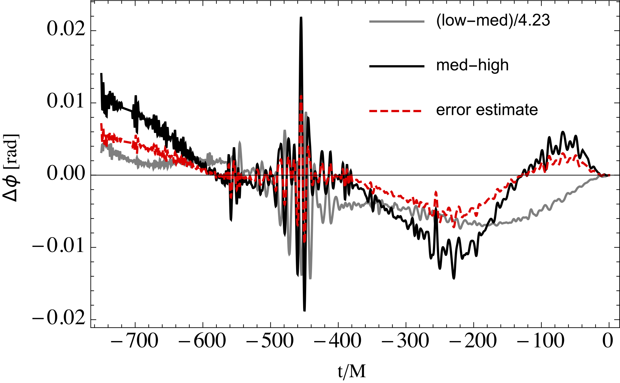
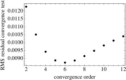
Even for the lowest-cost configuration (an equal-mass, non spinning binary), the computational cost prohibits a standard factor-of-two convergence test, and for many configurations there have been no clean demonstrations of convergence for any BBH code. Our confidence in NR results in general is based on the strong agreement between simulations from many independent codes, e.g., Refs. Hannam et al. (2009b); Ajith et al. (2012); Hinder et al. (2014). The results of a convergence test for a series of simulations for the $q=18$ nonspinning case are shown in Fig. 1. Due most likely to poorly resolved initial gauge dynamics and an initial burst of unphysical GW content (“junk radiation”), we have not been able to show convergence of the phase aligning at the beginning of the simulation, but we see reasonable sixth order convergence when aligning the $\ell=m=2$ GW signal near the merger at a frequency of $M\omega_{GW}=0.2$. Fig. 1 shows results from grid configurations with $(96,120,144)$ points in the innermost mesh refinement boxes, which dominate phasing errors and computational cost. Differences are scaled to sixth order convergence and we also show the error obtained as the difference of the highest resolution (144) and the Richardson-extrapolated result. Secular dephasing is very small, below $0.04rad$, and errors are dominated by oscillations and noise. Due to the oscillations and noise it is hard to decide by eye which convergence order is most consistent with the data, so we considered the RMS deviation

$$RMS^{2}=\frac{1}{t_{2}-t_{1}}\int_{t_{1}}^{t_{2}}\left((X_{1}-X_{2})/C(n)-(X_{2}-X_{3})\right)^{2}\,dt,$$ (9)

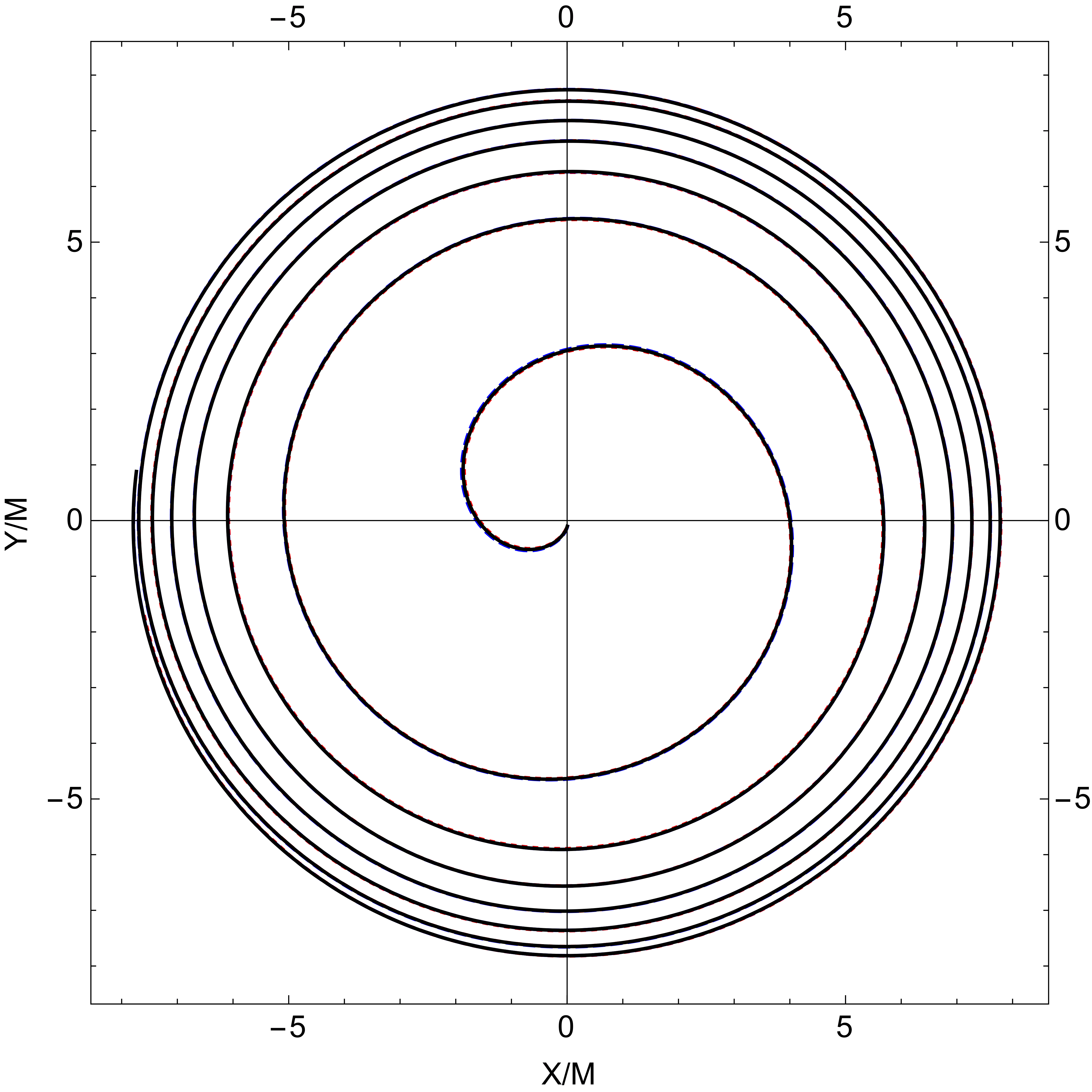
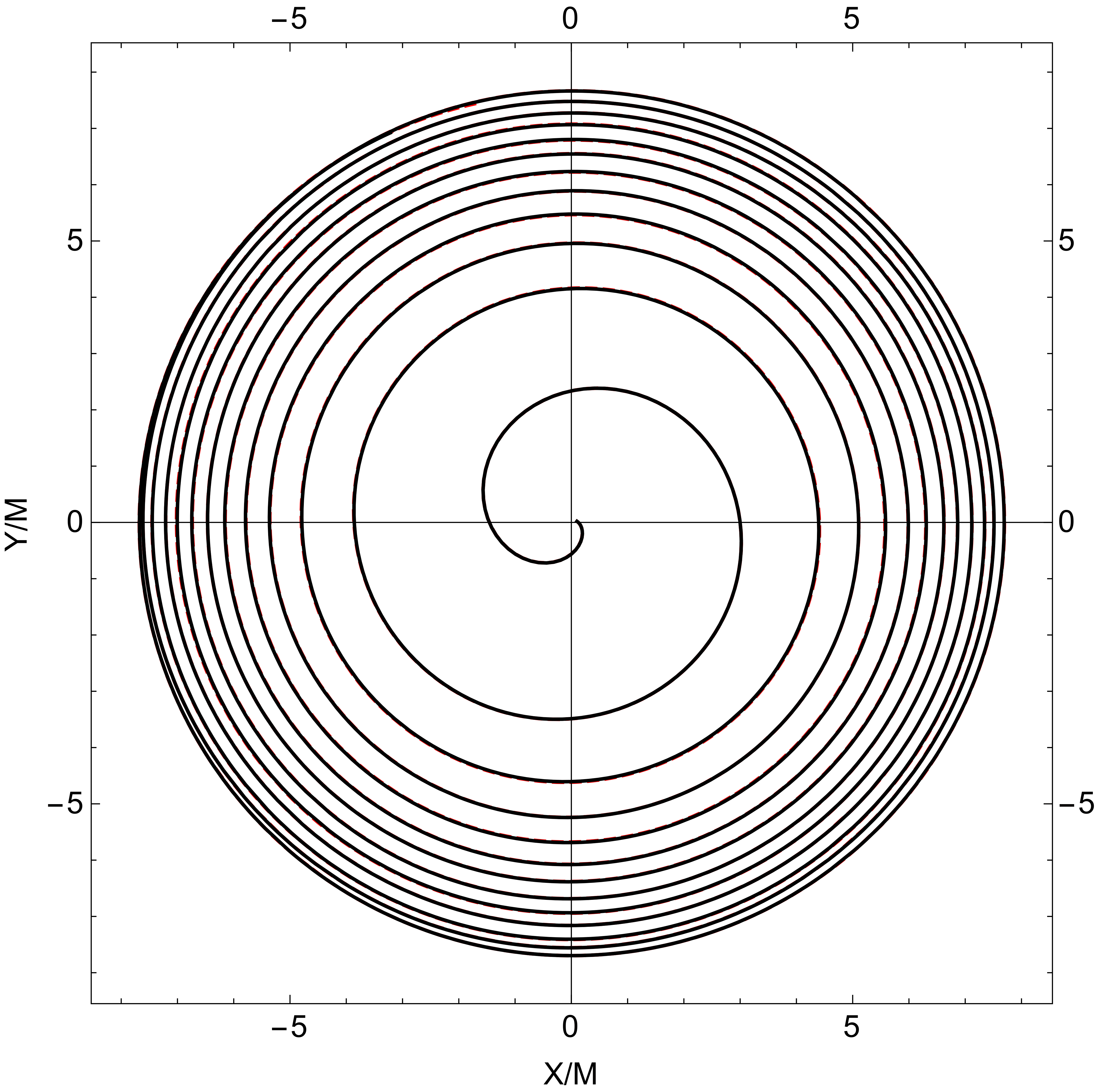
where the $X_{i}$ are the phases at resolutions $(96,120,144)$ aligned at $M\omega_{GW}=0.2$, $C$ is the rescaling factor corresponding to convergence order $n$, $t_{1}$ and $t_{2}$ are the minimal and maximal times shown in Fig. 1, and the unresolved pulse of noise between times $-500$ and $-400$ is set to zero. As can be seen in Fig. 2, the best-fitting convergence order is 6. In addition, in Fig.3 we show the that the orbital motion for the nonspinning convergence series and a low and medium resolution for a spinning $q=18$ case is practically indistinguishable for different resolutions. We have therefore not carried out a higher resolution run for the spinning case to save another $\approx 2$ million CPU hours, and we use the $96$ points resolution or better for the $q=18$ production runs.

Our NR waveforms only model the waveform from an astrophysical inspiral after some time $t_{0}$, when the influence of initial transients can be neglected. When processing a large number of waveforms, it is desirable to automatize the tedious procedure to find appropriate choices of $t_{0}$, and we thus need to understand initial transients in the waveform well enough to exclude them with a general algorithm. Two types of transients are of particular interest: the unphysical radiation content in the initial data, often referred to as “junk radiation”, and a transient component resulting from our conversion of $\psi_{4}$ to strain. In order to estimate the time on which junk radiation degrades the quality of the wave signal, we first determine the maximum of the amplitude of the junk radiation $t_{J}$ for the NR $\psi_{4}$ waveforms, and then add a multiple of the QNM damping period $T_{RD}=1/f_{damp}$ corresponding to the two initial BHs:

$$\Delta T_{J}=t_{J}+\sigma_{J}T_{RD}.$$ (10)

In order to convert $\psi_{4}$ waveforms to strain we use the fixed frequency integration algorithm Reisswig and Pollney (2011), which depends on the choice of cutoff frequency $f_{0}$. We choose this frequency as three quarters of the initial orbital frequency, which for the SXS data sets is determined from the included metadata, and for the BAM data sets is computed from the PN initial data parameters for the BH momenta. This value of the initial orbital frequency is cross-checked from the actual numerical waveform data by extrapolating the frequency evolution of the numerical waveform to the initial time by fitting to a fourth order polynomial in a time window starting after a time $T_{J}$. As can be expected on dimensional grounds, this procedure causes transients in the strain that persist for a time scale of the order of $1/f_{0}$. We thus define

$$\Delta T_{h}=\sigma_{h}/f_{0},$$ (11)

and discard numerical data before a time $t_{0}$, where

$$t_{0}=\max(\Delta T_{h},\Delta T_{J}).$$ (12)

For short waveforms of less than $3000M$ time to peak, we choose $\sigma_{J}=1,\sigma_{h}=2.5$, and for longer waveforms we choose $\sigma_{J}=3,\sigma_{h}=1.5$.

II.3 Post-Newtonian and effective-one-body descriptions

Our work uses PN waveforms in two ways: First, to construct “hybrid waveforms” that represent the complete inspiral-merger-ringdown of a binary system by appropriately gluing together PN and NR waveforms. Without restricting the generality of our approach we will carry out this procedure in the time domain (for an alternative frequency domain description see Santamaría et al. (2010)). Second, we will tune a frequency-domain PN approximant to the hybrid waveforms by calibrating higher order PN terms (which have not yet been computed in PN theory), in order to represent the inspiral regime of our final IMR waveform model.

Post-Newtonian perturbation theory provides a rich zoo of different approximants, which solve the Einstein equations up to a certain order of expansion, but may differ in higher order terms depending on how intermediate non-linear mathematical operations are performed. We will use standard quasi-circular non-precessing “Taylor-approximants”, described in Buonanno et al. (2009), in particular the TaylorT1, TaylorT2 and TaylorT4 time domain variants, and the TaylorF2 frequency domain version. These are consistently derived from an energy and flux which incorporate up to 3.5 PN order non-spinning terms (see for instance Buonanno et al. (2009)), 3.5 PN order in spin-orbit interaction Bohé et al. (2013a, b), 3PN order quadratic in spin Bohé et al. (2015), and 3.5PN order cubic in spin Marsat (2015).

Terms corresponding to higher PN order may also be added in order to conform with a particular form of the energy, flux, or some other property of the binary. In our work we will in particular use models derived from the very successful EOB description Buonanno and Damour (1999, 2000). In particular, we will use the SEOBNRv1 Taracchini et al. (2012) and SEOBNRv2 Taracchini et al. (2014) models in two forms, the proper SEOBNRv1/v2 waveform model, which is calibrated against numerical relativity waveforms from the SXS catalogue SXS , and an uncalibrated version, which we refer to as SEOBv1/v2, where all terms calibrated to NR have been set to zero. In detail, we have applied the following changes to the SEOBNRv2 model Taracchini et al. (2014) to obtain the uncalibrated waveforms which we will refer to as SEOBv2: In the EOB Hamiltonian we have set the 4.5PN spin-orbit adjustable parametr $d_{SO}$ and the 3-PN spin-spin parameter $d_{SS}$ to zero, and we for non-spinning correction only keep the mass-ratio independent term in the parameter $K$, thus $K=1.712$. The 3PN term added to the quantity $\delta_{2}2$ in the factorized waveforms is also set to zero, as are all NQC corrections. Furthermore, in order to keep the implementation of the SEOBNRv2 in the file LALSimIMRSpinAlignedEOB.c LAL library The LIGO Scientific Collaboration (2015) from crashing, the parameter tStepBack was changed from tStepBack = 100.*mTScaled to tStepBack = 300.*mTScaled. While this work has been in progress, it has been found in Szilágyi et al. (2015), that an (independent) uncalibrated version of SEOBNRv2 shows excellent agreement with a 125-orbit-long mass-ratio 7 non-spinning waveform.

II.4 Hybrids

We construct hybrid waveforms, where the early time behaviour is described by a PN approximant, and the late time behaviour by a NR waveform, by essentially standard procedures. See Refs. Ajith et al. (2008); Boyle (2011); MacDonald et al. (2011); Ajith et al. (2012) for summaries of different methods in the literature, and Ref. Bustillo et al. (2015) for a detailed description of our specific procedure, which we briefly summarize here.

First, we note that any non-precessing-binary waveform $h(t)$ we consider represents an equivalence class of waveforms, which correspond to a binary with the same masses and spins, and only differ by a relative time shift, a relative rotation, and the sense of their orbital rotation (i.e. the sign of the frequency $\omega$). Without restricting generality we will choose the frequency as positive. The PN and NR strains $h^{PN/NR}$ will then be related by

$$h_{22}^{PN}(t)=e^{i\varphi_{0}}h_{22}^{NR}(t+\Delta t).$$ (13)

In order to find good parameters $\Delta t$ and $\varphi_{0}$, we fix an initial time $t_{0}$ and fitting window length $T$, and minimize the quantity

$$\Delta(\Delta t;t_{0},T)=\int_{t_{0}}^{t_{0}+T}\left(\omega^{PN}(t)-\omega^{NR}(t+\Delta t)\right)^{2}dt,$$ (14)

with respect to the time shift $\Delta t$. Alternatively we replace $\omega$ by $\phi$ to obtain a consistency and robustness check, which is particularly useful when automatically processing tens of waveforms as we do. Our original choice of $\omega$ has the advantage of not depending on $\varphi_{0}$. Other authors have replaced $\omega$ by $h$ MacDonald et al. (2011) in the integrand, here we only use phase and no amplitude information in order to avoid the influence of amplitude errors. In Bustillo et al. (2015) we have checked that the window length $T$ that corresponds to four GW cycles (two orbits) is sufficient to average out oscillatory waveform artefacts mostly due to residual eccentricity. In order to find an appropriate phase shift $\varphi_{0}$ for given $\Delta t$ from the minimization of Eq. (14), we align the phases at the middle of the matching window.

The hybrid waveform is then defined as,

$$h(t)=\omega^{-}_{(t_{0},t_{0}+T)}e^{i\varphi_{0}}h^{PN}(t+\delta t)+\omega^{+}_{(t_{0},t_{0}+T)}h^{NR}(t),$$ (15)

where $\omega^{-/+}$ are linear transition functions over the time window $t\in[t_{0},t_{0}+T]$.

The crucial step, however, when “glueing” PN to numerical waveforms is to consistently align them at some reference frequency, where we choose their time coordinates and phases to coincide. If the waveforms are identical, the relative time (and phase) shift between them will be independent of the matching frequency. We are interested in the case where the waveforms are different, and where we have the choice of PN approximant, e.g. one discussed in Sec. II.3, to attach to a particular numerical waveform. For non-identical waveforms the relative time-shift between the PN and NR descriptions will depend on the frequency where the two waveforms are compared or matched together. A preferred PN approximant would exhibit a time shift relative to the NR waveform which depends only negligibly on time. In order to find the best-matching PN approximant, we compute the hybridisation time shift as a function of matching frequency as follows. We consider the time dependent frequencies $\omega_{PN}(t)$ and $\omega_{NR}(t)$. We can invert these functions numerically, e.g. by evaluating them for a series of time steps, and then interpolating inverse functions of $t(\omega)$. To compute the time shift we then compute the difference

$$\Delta t=t_{PN}(\omega)-t_{NR}(\omega).$$ (16)

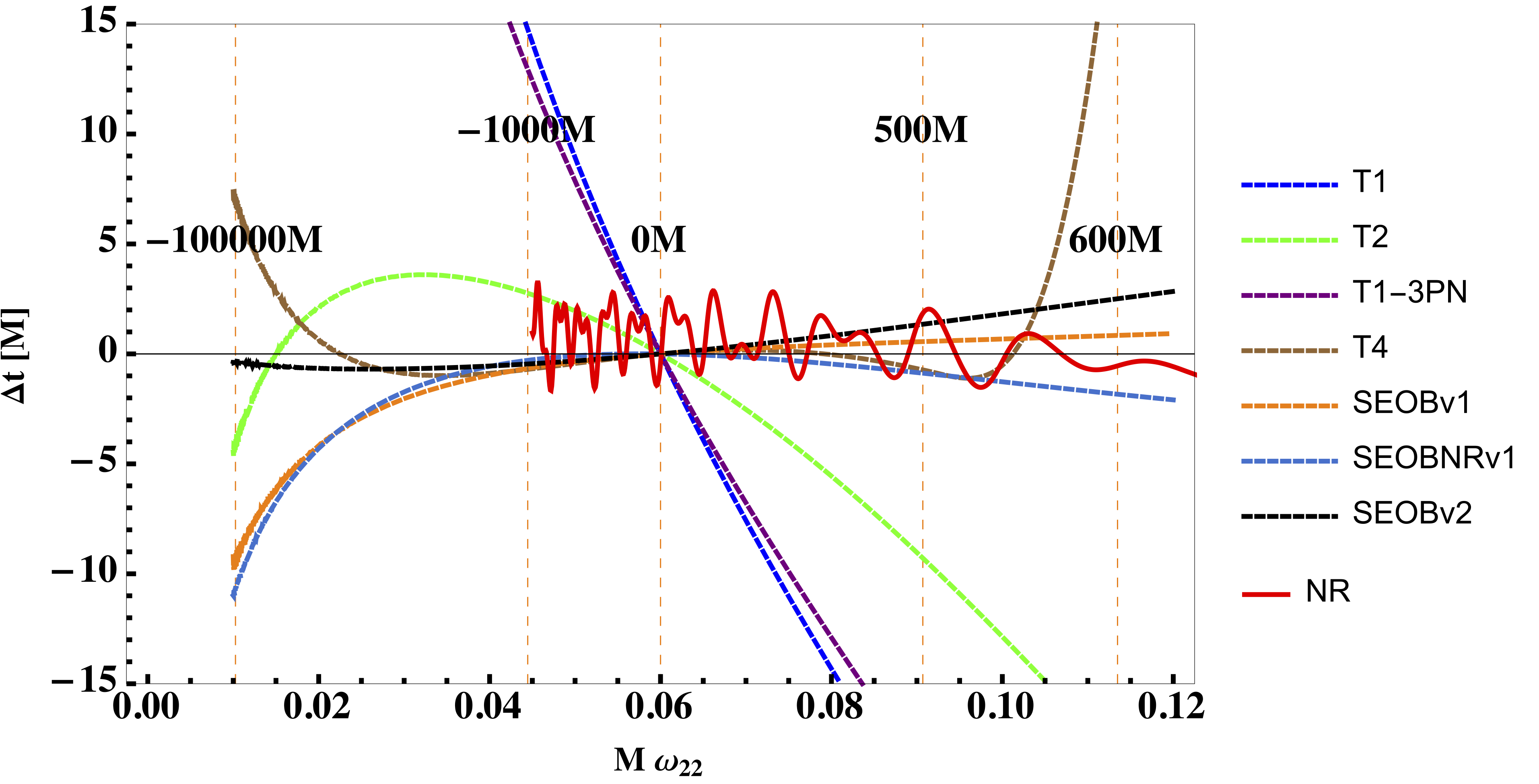
The results are displayed in Figs. 4-5. First, in Fig. 4 we consider the equal mass non-spinning case, where we however use SEOBNRv2 and not the NR results as the reference waveform, in order to reduce the effect of oscillations in the NR result due to residual eccentricity. One can see that the NR waveform SXS:BBH:0001 from the SXS catalogue, the uncalibrated SEOBv2 and TaylorT4 are very close to each other over the frequency range of the NR waveform. SEOBNRv2 and SEOBv2 are close over the whole frequency range plotted, $0.01\leq M\omega_{22}$.

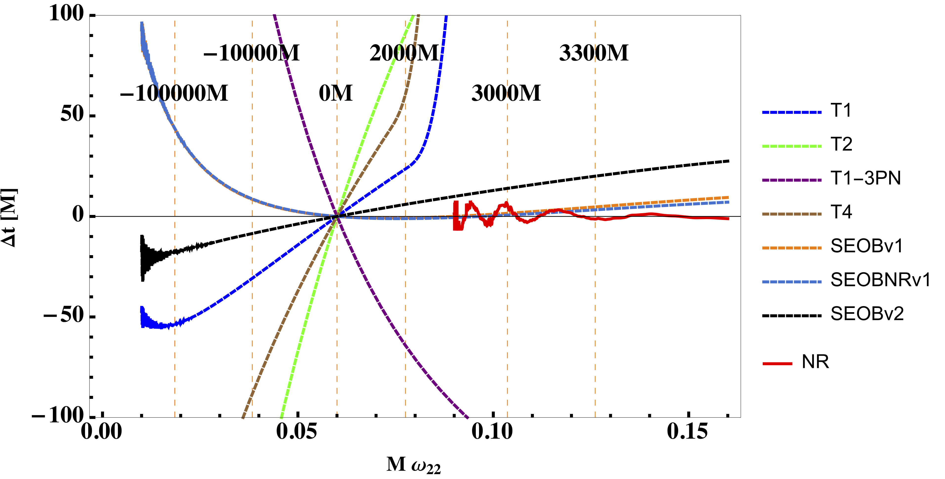
In the left panel of Fig. 5 we consider the BAM mass-ratio 18 case with a mild dimensionless spin of $\chi_{1}=0.4$ parallel to the orbital angular momentum on the bigger BH, and a non-spinning smaller hole. Again we use SEOBNRv2 as the reference waveform. We see that the NR and SEOBNRv2 waveforms agree well over the common frequency range, and the approximant that performs next best is the uncalibrated SEOBv2. Note that now the $\Delta t$ time scales are much larger than in Fig. 4, and that the standard PN approximants perform markedly worse in comparison to the NR than the SEOB(NR)v2 waveforms.

Figure 4: Time shift $\Delta t$ according to Eq. (16) as a function of wave frequency $M\omega$ for the case of non-spinning $q=1$, using SEOBNRv2 as the reference waveform and SXS:BBH:0001 from the SXS catalogue as the NR waveform. As is well known, the SEOBNRv2 model and TaylorT4 are very close to the NR result in this case. Uncalibrated SEOBv2 (uncalibrated SEOBNRv2) is also very close, while TaylorT1, TaylorT1 cut off at 3PN order, and TaylorT2 show significant dephasing. The SEOBNRv1 and SEOBv1 (uncalibrated SEOBNRv1) show rather similar performance, with good agreement with NR, and disagreement with SEOBNRv2 at lower frequencies.

Figure 5: Left panel: Time shift $\Delta t$ according to Eq.16 as a function of wave frequency $M\omega$ for the case of mass ratio 18 with spins $\{0.4,0\}$ with SEOBNRv2 as the reference waveform. The PN/EOB waveforms start at $M\omega=0.01$. Right panel: Same analysis for an equal mass binary with equal spins $\chi=0.98$. Tthe NR waveform is SXS:BBH:0172 from the SXS catalogue, see Table 3. SEOBNRv1/SEOBv1 are not shown for this case, since the model is not valid for high spins parallel to the orbital angular momentum.

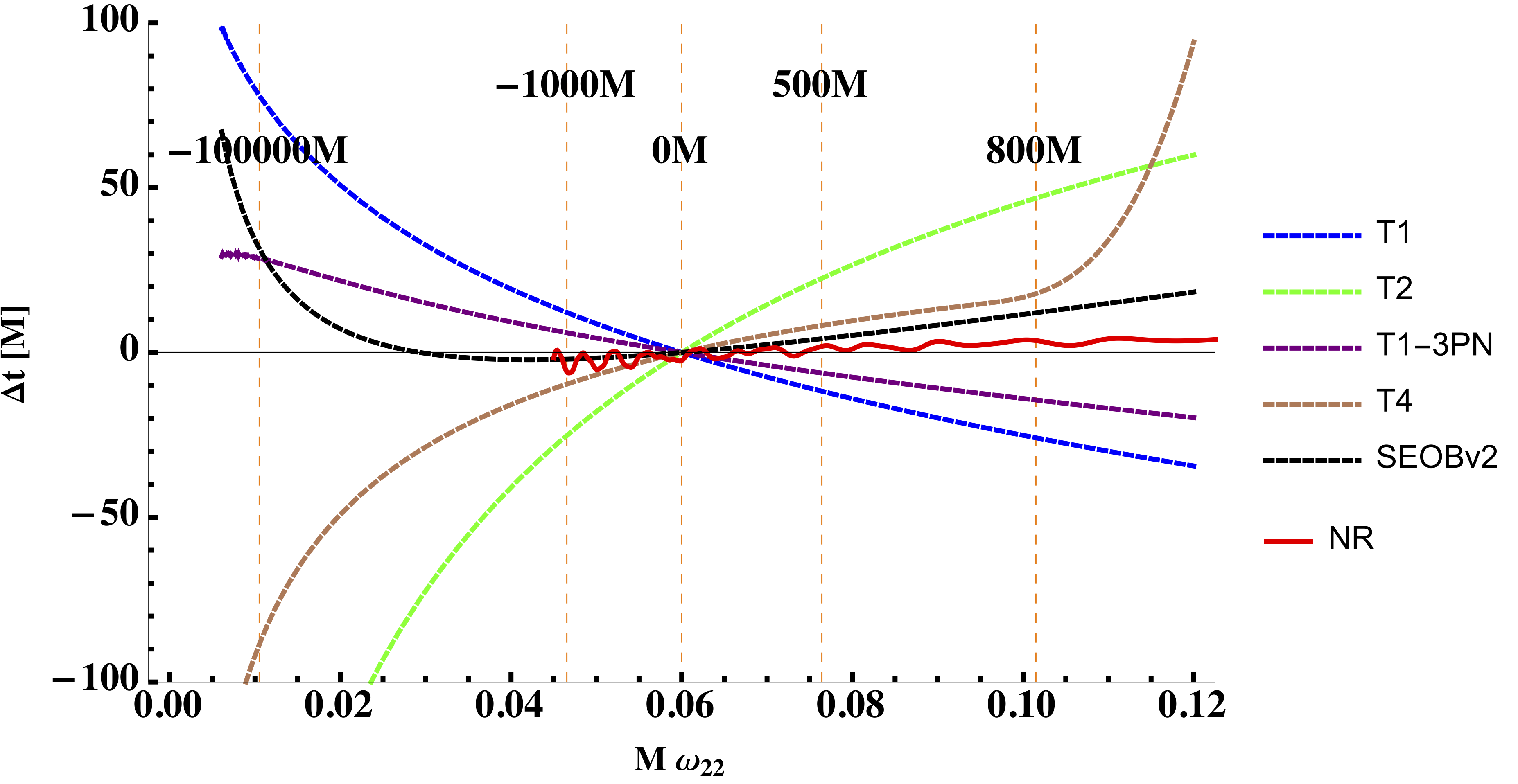
In the right panel of Fig. 5 we finally consider again equal masses, but now with large spins of $\chi_{1}=\chi_{2}=0.98$ parallel to the orbital angular momentum. The NR waveform is SXS:BBH:0172, produced with the SpEC code. The dephasing between the NR waveform and SEOBNRv2 is again rather small, although significantly larger than in the nonspinning case. The SEOBv2 waveform is the approximant closest to SEOBNRv2 for waveforms not longer than $10^{5}M$. For lower frequencies, TaylorT1 cut off at 3PN order is closer to SEOBNRv2, but all other approximants show significantly larger differences.

The time-shift analysis discussed here for three examples has also been carried out for a number of other cases, with similar results, which will be presented in more detail in a separate paper. The conclusion for our current work is that in the frequency regime relevant for hybridisation, SEOBv2 uncalibrated EOB waveforms are almost as close to NR results as the calibrated EOB model, and at low frequencies are typically closer to SEOBNRv2 than any other approximant at 3.5PN order. In Ref. Bustillo et al. (2015) we have shown a similar result, where we have applied a similar analysis to compare TaylorT1, TaylorT4 and SEOBNRv1 to the BAM non-spinning NR waveform at mass ratio 18, and have found that SEOBNRv1 is far superior for hybridization.

In this work we will therefore construct all our hybrid waveforms, which form the input to our phenomenological modeling, with the SEOBv2 model. We are thus able to calibrate an inspiral model that is independent from the calibration process performed for SEOBNRv2, which will allow valuable cross checks.

Frequency domain strain hybrids are constructed by sampling the time domain hybrid with equispaced time steps, and aligning all waveforms such that the value of the time coordinate and phase at the peak amplitude vanish. The waveforms are then zero-padded to all start at a time $t_{\rm start}$ and all end at a time $t_{\rm end}$, where $t_{\rm start}$ is significantly smaller than the beginning of the numerical EOB data, and $t_{\rm end}$ is chosen at several hundred $M$ after the amplitude peak. Different batches of hybrids have been produced for comparisons, with the time-step typically chosen as $0.5M$ or $1M$.

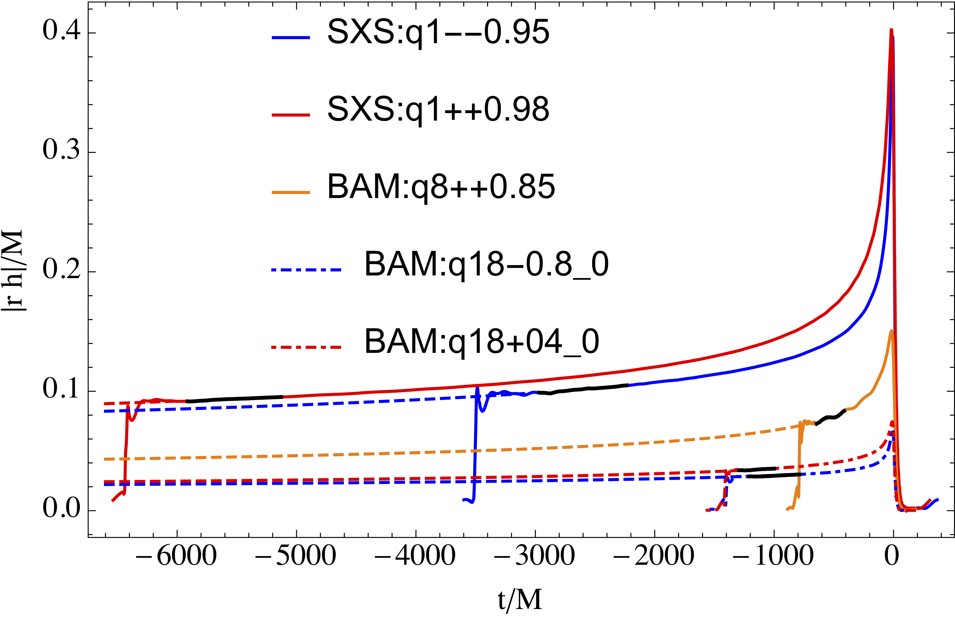
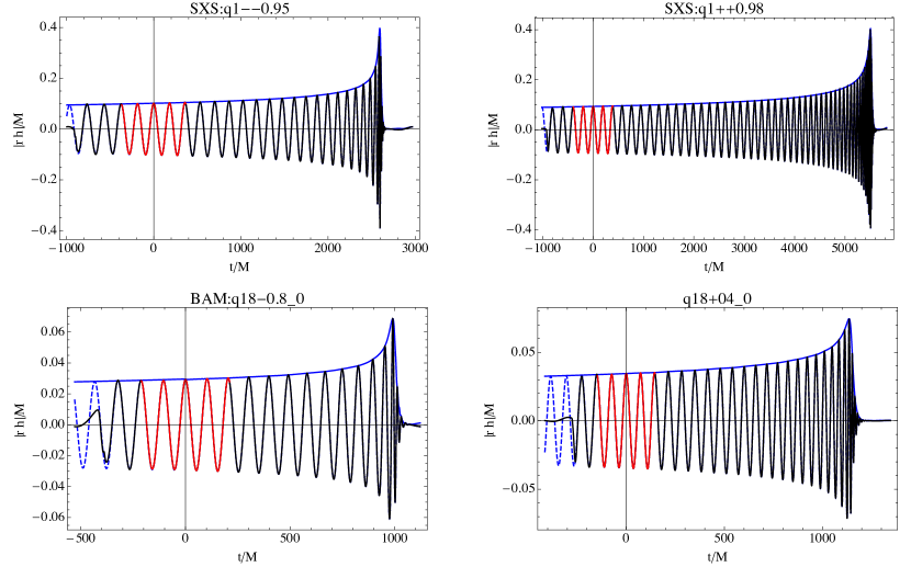
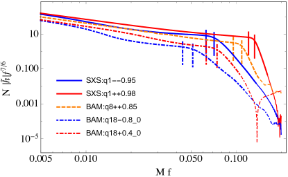
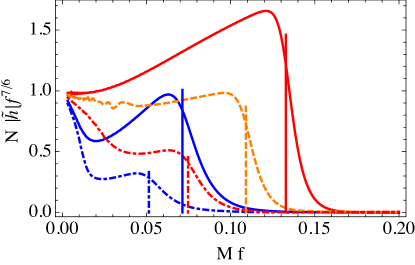
The time-domain amplitude for selected hybrids is shown in Fig. 6. The strain for the same cases is shown in Fig. 7, and the Fourier-domain amplitudes are shown in Figs. 8.

Figure 6: Time domain amplitude of configurations at the corners of our parameter-space coverage, aligned at merger, showing both the NR waveform and the hybrid (marked as dashed lines). Thick black lines mark the hybridization regions.

Figure 7: Real part of the time domain strain of corner cases, time coordinate is set to zero at the mid-frequency of the hybridization region, which is shown in red.

Figure 8: Fourier domain amplitude of corner cases and ringdown frequency. In the left panel, the thick lines indicate the part of the NR waveform that was used in the final hybrid, while data indicated by a thin line contained noise or other spurious artifacts, and was discarded. The vertical lines indicate the peak of the amplitude, and the ringdown frequency $f_{RD}$. In the right panel the $f^{-7/6}$ leading-PN-order amplitude has been scaled out to illustrate detailed features of the Fourier-domain amplitude through merger and ringdown.

III Modeling the final state

While it has not been rigorously proven within general relativity, the final state of the coalescence observed in all NR calculations is a single perturbed Kerr BH. The complex frequency of the “quasinormal” ringdown provides two key pieces of information for modelling the GW signal, and can be computed directly as a function of the final mass and spin. As a first step to model waveforms, we will thus model the final state and provide simple analytical fitting formulas for the radiated energy and final spin as a function of symmetric mass ratio and an effective spin parameter. These cover a wider parameter space than previous work in the literature; see Refs. Barausse and Rezzolla (2009); Hemberger et al. (2013b); Healy et al. (2014); Zlochower and Lousto (2015) and references therein. This will also illustrate how we construct analytical fits across the parameter space, and similar procedures will be used afterwards in our waveform modelling. The main goal of our approach to model the final state is to construct accurate explicit expressions, which are therefore fast to evaluate and easy to generalize to larger calibration data sets.

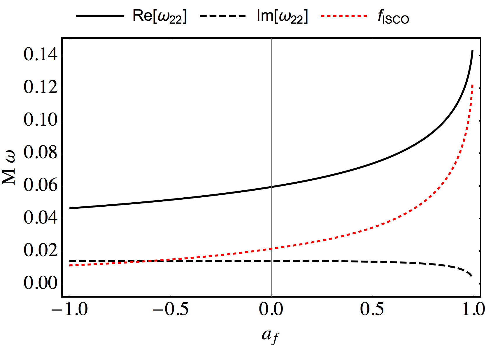
To determine the dimensionless ringdown frequency $M\omega_{RD}$ as a function of $a_{f}$, we have interpolated the data set in Refs. Berti et al. (2009); Berti, Emanuele and others (2015). These well known functions are shown in Fig. 9, together with the wave frequency corresponding to a test particle on innermost stable orbit (ISCO) Bardeen et al. (1972) of Kerr spacetime. One can see that the steepest functional dependence happens for large positive spins.

To calculate the dimensionful ringdown frequency of the binary, loss of energy during inspiral needs to be accounted for as

$$\omega_{RD}=\frac{(M\omega_{RD})}{M_{f}}=\frac{(M\omega_{RD})}{M-E_{\mbox{rad}}},$$ (17)

and we need to model the radiated energy $E_{\mbox{rad}}$ in addition to the final Kerr parameter.

Figure 9: Real (oscillatory)and imaginary (damping) part of the ringdown frequency as a function of the final Kerr parameter $a_{f}$. A positive sign denotes a final BH parallel to the initial orbital angular momentum, and negative sign antiparallel.

We have used final spin and radiated energy results from the following 106 data sets: 15 new BAM cases at mass ratios 2, 3, 4, 8, 18, 5 old BAM cases at mass ratio 4 from published in Pürrer et al. (2013) (used only for the final spin), 50 cases from the SXS catalogue  SXS , and 36 cases from the RIT group Healy et al. (2014). For the RIT runs, two type of results are given, derived from the isolated horizon formalism and from the radiation, and we use the isolated horizon quantities due to the lower error bars quoted. We do not use the mass-ratio 10 results from the RIT data set, since the quoted result for the radiated energy differs from ours and the numerical fit by a factor of two and is possibly a misprint.

III.1 Final spin

Before merger, the total angular momentum can be expressed in terms of the individual BH spins $\vec{S}_{i}$, which for our purposes change only negligibly during inspiral, and the orbital angular momentum $\vec{L}$ as,

$$\vec{J}=\vec{L}+\vec{S}_{1}+\vec{S}_{2}.$$ (18)

Due to symmetry all angular momentum vectors are orthogonal to the orbital plane and the only non-zero component is the $z$-component. For simplicity of notation, we therefore drop the vector notation, and write $J,S_{i}$, etc., for the $z$-component. We seek to approximate $J$, $L$, and correspondingly the final Kerr parameter $a_{f}=J_{f}/M_{f}^{2}$ through a function of the mass ratio and a single effective spin parameter. Given that Eq. (18) depends trivially on the sum of the individual spins, we attempt the approximation

$$\vec{J}_{f}\approx\vec{J}_{f}(\eta,\vec{S}),\quad\vec{S}=\vec{S}_{1}+\vec{S}_{2}.$$

In the infinite mass ratio limit, $\eta=0$, the final spin coincides with the spin of the larger BH,

$$J_{f}(\eta,S_{1},S_{2})=S_{1}=S,\quad a_{f}(\eta,\chi_{1},\chi_{2})=\chi_{1}.$$ (19)

We will frequently use a rescaled version of our total spin $S=S_{1}+S_{2}$ to $\hat{S}=S/(1-2\eta)$, for which $-1\leq\hat{S}\leq 1$, consistent with the extreme Kerr limit.

The data points are shown in Fig. 10. As can be seen, our waveform coverage is densest at equal mass and sparser at higher mass ratios. To produce an analytical fit, we first inspect the data set displayed in Fig. 10, and in particular the non-spinning and equal mass subsets. We find that fourth order polynomials in $\eta$ and $S$ produce accurate fits for the two subsets, and we fix the linear term in $\eta$ by a Taylor expansion around the extreme mass ratio limit as in Rezzolla et al. (2008),

$$a_{f}=2\sqrt{3}\eta+\mbox{higher order in $\eta$ and spins}.$$ (20)

In order to cover the whole parameter space we extend the ansatz by terms quadratic in $\eta$ and quartic in the total spin $S$ to

$$a_{f}^{eff} = f_{00}+S+\eta\sum_{i=0,4}\frac{f_{1i}}{i!}S^{i}$$ (21)

$$+\eta^{2}\sum_{i=0,4}\frac{f_{2i}}{i!}S^{i}+f_{30}\eta^{3}+f_{40}\eta^{4}.$$

After fixing coefficients for consistency with the nonspinning and equal mass cases, the only coefficients left to fit are the 4 numbers $(f_{11},f_{12},f_{13},f_{14})$. The result is,

$$a_{f}^{eff}(\eta,S)=S+2\sqrt{3}\,\eta-4.399\,\eta^{2}+9.397\,\eta^{3}-13.181\,\eta^{4}$$

$$+(-0.085\,S+0.102\,S^{2}-1.355\,S^{3}-0.868\,S^{4})\,\eta$$

$$+(-5.837\,S-2.097\,S^{2}+4.109\,S^{3}+2.064\,S^{4})\,\eta^{2}$$ (22)

RMS errors are $6.8\times 10^{-3}$, and $2.4\times 10^{-3}$ when comparing the fit with the equal spin subset. We also note that this fit respects the Kerr limit, i.e., $a_{f}^{\rm eff}|\leq 1$.

Figure 10: Final Kerr parameter from Eq. 22 plotted as a function of symmetric mass ratio and total spin $\hat{S}$. Black dots mark data points with equal spins, grey dots unequal spins.

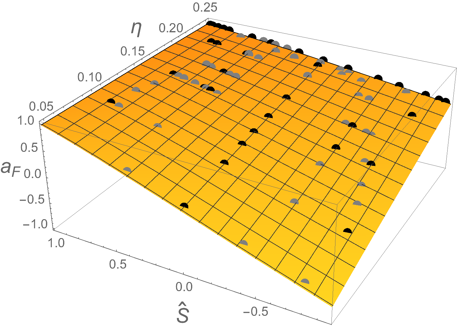
III.2 Radiated energy

The data points for radiated energy are shown in Fig. 11, together with the effective single spin fit we will now discuss. Inspecting the plot, clearly, a polynomial in the symmetric mass ratio and the effective spin will not provide the ideal model, and a rational function model comes to mind. Also, as in the final spin case, clearly a reliable accurate model of the whole parameter space would require further data points for large spins.

It turns out that after factoring out a fit to the nonspinning subset, the radiated energy depends only rather weakly on the symmetric mass ratio. We find that the non-spinning radiated energy, $E_{rad}^{NS}(\eta)$, is very well captured by a fourth order polynomial, at a RMS of $3.5\times 10^{-5}$,

$$E_{rad}^{NS}(\eta)=0.0559745\eta+0.580951\eta^{2}-0.960673\eta^{3}+3.35241\eta^{4}.$$ (23)

As can be seen in Fig. 10, the effective spin $\hat{S}$ works reasonably well for the radiated energy. We model the dependence on the spin $\hat{S}$ through a simple rational function, where the numerator and denominator are linear in spin and quadratic in symmetric mass ratio, with some experimentation having gone into making a choice for which the nonlinear fitting procedure converges well, and the result has no singularities due to vanishing denominator. The result of the fit, with a RMS error of $4\times 10^{-4}$ is,

$$\frac{E_{rad}}{M_{ini}}=E_{rad}^{NS}(\eta)\frac{1+\hat{S}\left(-0.00303023-2.00661\eta+7.70506\eta^{2}\right)}{1+\hat{S}\left(-0.67144-1.47569\eta+7.30468\eta^{2}\right)}$$ (24)

Figure 11: Radiated energy according to fit Eq. 24 plotted as a function of symmetric mass ratio and total spin $\hat{S}$. Black dots mark data points with equal spins, grey dots unequal spins.

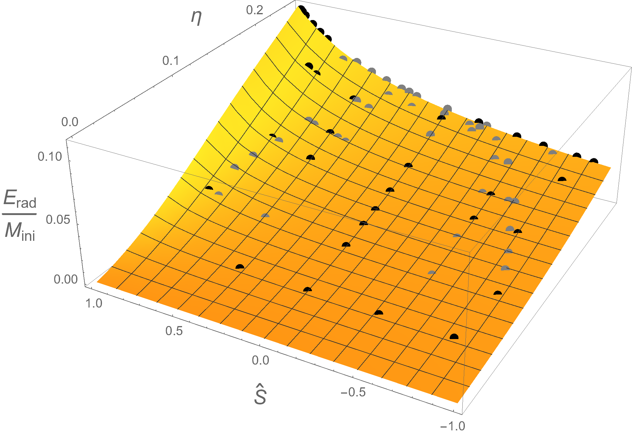
IV Waveform anatomy and model

IV.1 Waveform anatomy

IV.1.1 Amplitude

The waveform anatomy in the time domain has been studied extensively, and combined with EOB resummation techniques of PN results has given rise to the family of EOB-NR waveform models Buonanno et al. (2007); Damour et al. (2008); Pan et al. (2011); Damour et al. (2013); Taracchini et al. (2014); Nagar et al. (2015). One may distinguish three phases without sharp boundaries: (i) a long inspiral with slowly increasing amplitude, where the amplitude scales as $M\eta\omega^{2/3}$ in the low frequency limit, and the coalescence time as $\omega^{-8/3}/\eta$, (ii) an “extended-merger” characterised by a rapid increase in amplitude and frequency; (iii) followed by a damped sinusoidal ringdown. The Fourier transformation to obtain the frequency domain waveform can in general not be carried out analytically. In the low-frequency regime however, the stationary phase approximation (SPA) can be used to analytically obtain an approximate Fourier transform, which is used in particular to obtain the TaylorF2 PN approximant as a closed-form expression. Following the procedure outlined for example in Section 3 of Ref. Santamaría et al. (2010) we obtain the SPA amplitude using the TaylorT4 form of the energy balance equation. The Fourier domain amplitude, $\tilde{A}_{22}$, is then given in terms of the time domain amplitude $A_{22}$ and second phase derivative $\ddot{\phi}$ evaluated at the Fourier variable $t_{f}=(2\pi f/m)^{2/3}$, where $m=2$ for the dominant harmonic we consider,

$$\tilde{A}_{22}(f)=A_{22}(t_{f})\sqrt{\frac{2\pi}{m\ddot{\phi}(t_{f})}}\,.$$ (25)

In particular, to leading order the Fourier amplitude is,

$$|\tilde{h}_{22}|=A_{0}f^{-7/6}(1+O(f^{2/3})),\qquad A_{0}=\sqrt{\frac{2\,\eta}{3\,\pi^{1/3}}}.$$ (26)

In order to better emphasize the non-trivial features of the amplitude, we rescale our numerical data sets by the factor ${f^{7/6}}/{A_{0}}$, to normalize all amplitudes to unity at zero frequency as shown in Fig. 8. We see a structure that is sufficiently rich that a single analytical expression for the entire frequency range is difficult to achieve in terms of elementary (and thus computationally cheap) functions. Our strategy will thus split our description into an inspiral part, which models the waveform as higher order corrections to PN expressions, a merger-ringdown part which builds upon the knowledge of the final state, and an intermediate part which describes the frequency regime which can not be based directly upon PN or the final state.

Regarding the merger-ringdown, a crude time domain model, which can be Fourier-transformed analytically, is a sine-Exponential, which is symmetric around the peak amplitude:

$$h(t)=e^{2\pi(if_{\text{RD}}t-f_{\text{damp}}|t|)}\qquad f_{\text{RD}},\,f_{\text{d}amp}\in R.$$ (27)

The Fourier transform (4) yields a Lorentzian,

$$\tilde{h}(\omega)=-\frac{1}{\pi}\frac{f_{\text{damp}}}{(f-f_{RD})^{2}+f_{\text{damp}}^{2}},$$ (28)

which only falls off as $f^{-2}$ at large frequencies as expected from Eq. (8), due to the fact that the original time domain waveform $h(t)$ is only $C^{0}$ at the peak. Despite its oversimplification, in particular the unphysical symmetry around the peak, and the incorrectly slow falloff at high frequency, the Lorentzian has provided a valid model for frequencies higher than the ringdown frequency in PhenomA/B/C models. Looking at Fig. 8, the expected roughly exponential drop at high frequencies are clearly visible.

A natural extension of the Lorentzian ansatz used in the previous Phenom models, is to model the merger-ringdown amplitude $A_{MR}$ by multiplying the Lorentzian by an exponential as

$$\frac{A_{\text{MR}}}{A_{0}}=\gamma_{1}\frac{(\gamma_{3}f_{\text{damp}})}{(f-f_{\text{RD}})^{2}+(f_{\text{damp}}\gamma_{3})^{2}}e^{-\lambda(f-f_{\text{RD}})}\,.$$ (29)

In order to find best fit parameters, we use Mathematica’s NonlinearModelFit function. To achieve robust convergence of the nonlinear least squares fit, we redefine

$$\lambda=(\gamma_{2}/(f_{\text{damp}}\gamma_{3})),$$

to achieve a magnitude of order unity for the new free parameter $\gamma_{2}$. The merger-ringdown amplitude model thus has three free parameters that are fit from numerical waveform data, and the real and imaginary part $f_{\text{RD}},f_{\text{damp}}$ of the QNM ringdown frequency are computed from the known fits for final spin and mass from Eqs. (22) and (24) and the known dependence of the QNM frequencies on the dimensionless Kerr parameter shown in Fig.9. Interestingly, it turns out that $\gamma_{3}\in[1.25,1.36]$, i.e., it has a very narrow dynamical range and could also be approximated as constant $\gamma_{3}\approx 1.3$.

The exponential factor in our ansatz Eq. (29) shifts the amplitude peak from $f_{\rm RD}$ for the Lorentzian to

$$f_{\rm max}=\left|f_{\text{RD}}+\frac{f_{\text{damp}}\gamma_{3}\left(\sqrt{1-\gamma_{2}^{2}}-1\right)}{\gamma_{2}}\right|.$$ (30)

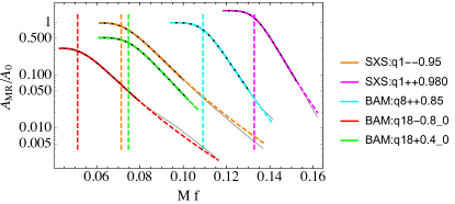
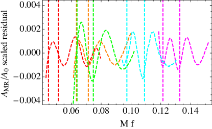
An appropriate frequency range for fitting the model Eq. (29) to numerical data can be determined as follows. At the large frequency end, we first discard frequencies with significant numerical noise by the following heuristic procedure: We multiply the amplitude with $f^{p}$, where we find that $p\approx 4$ works well. For physically accurate data we expect a monotonic decrease for the rescaled amplitude. Due to unphysical artefacts however, a minimum will appear, and we discard all frequencies higher than the one of the minimum. The result can be seen in Fig. 8. While no “fine-tuning” is required, a good choice of frequency range for model fitting will not only increase the accuracy of the fit, but also lead to smoother variation over the BH parameter space of mass ratio and spins, which will be essential when constructing a phenomenological model in Paper 2 Khan et al. (2015). At low frequency we find that the fit is only good up to the peak $f=f_{\rm max}$, while at large frequencies, where the amplitude is already very small, we need to control contamination from numerical artefacts. Also, to avoid boundary effects, we extend the fitting range to slightly smaller frequencies than $f=f_{\rm max}$. We find that two strategies work well: specifying the fitting range in terms of multiples of the ringdown frequency and the numerically determined local maximum, e.g. using the range $(f_{\rm max},1.2f_{\rm RD})$, or using the width of the Lorentzian, e.g. as $(f_{\rm max}-f_{\rm damp}/2,f_{\rm RD}+2f_{\rm damp})$. Fits and residuals for the latter choice are shown in Figs. 12 and 13.

Since the merger-ringdown amplitude model Eq. (29) thus covers a frequency range which will be covered even by the shortest NR simulations of BH mergers, simulations only need to be sufficiently long to control the systematic error of residual eccentricity, to avoid low frequency artefacts from the Fourier transformation, and to clearly separate the unphysical radiation content discussed in Sec. II.2 from the physical part of the signal.

Figure 12: Comparison of ringdown fit with numerical data for 5 “corner cases” as indicated in the legend. Full thin lines indicate raw numerical data, full thick lines indicate numerical data with a heuristic cutoff to remove noise at high frequencies, dashed lines indicate the best fit to ansatz Eq. 29.

Figure 13: Residuals between numerical data and best fits for the data shown in Fig. 12.

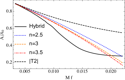
Returning now to the inspiral, it is natural to model the early frequency behaviour as a modification of the known closed-form PN expression corresponding to the TaylorF2 approximant. As can be seen in Fig.8, modeling the pre-merger amplitude is particularly challenging for negative spins (and higher mass ratios), where the amplitude shows a very sharp drop, whereas for positive spins the frequency dependence is rather shallow. In the PhenomC model Santamaría et al. (2010) the amplitude was taken directly in the form of Eq. (25) as resulting from the SPA calculation. We find however that the variation of the phenomenological parameters is smoother if instead of using the SPA amplitude defined in Eq. (25) we re-expand the ratio of the separate PN expansions of $A_{22}(t_{f})$ and $\ddot{\phi}(t_{f})$. A comparison of different forms of the the TaylorF2 amplitude is displayed in Fig. 14 for the $q=18$ case with the larger black hole spinning at $\chi_{1}=-0.8$. One can see that the re-expanded forms are closer to the hybrid data. This does not hold across the parameter space, but it is for the negative spin cases like the one shown here where the difference is particularly large.

Figure 14: Different forms of the TaylorF2 amplitude, rescaled as in the right panel of Fig. 8, are displayed for the $q=18$ case with the larger black hole spinning at $\chi_{1}=-0.8$. Shown are the numerical data of the hybrid waveform, the absolute value of the complex TaylorF2 amplitude from Eq. (25), and the real part of the TaylorF2 amplitude after re-expanding to $n=2.5,3,3.5$ PN order. It can be seen that the re-expanded forms are closer to the hybrid data. Taking the real part or absolute value of expressions makes no significant difference for the case and frequency range shown.

To perform the re-expansion we set the logarithmic terms to zero and retain the complex terms in $A_{22}$. Based upon comparisons to the hybrid it was only necessary to keep terms to $\mathcal{O}(f^{2})$, which is equivalent to a consistent truncation at 3PN order. In the final result we use only the real part of this expression; the contribution from the imaginary part is negligible. The re-expanded SPA amplitude is given by,

$$A_{\text{PN}}(f)=A_{0}\sum_{i=0}^{6}\mathcal{A}_{i}(\pi f)^{i/3}\,,$$ (31)

where $A_{0}$ is the leading order $f^{-7/6}$ behaviour. We then calibrate the next three natural terms in the PN expansion,

$$A_{\text{Ins}}=A_{\text{PN}}+A_{0}\sum_{i=1}^{3}\rho_{i}\,f^{(6+i)/3}.$$ (32)

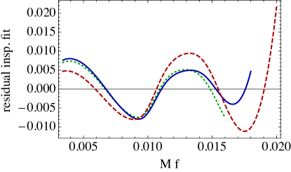
The choice of 3 terms resulted as a compromise between accuracy and simplicity, and adding more terms may be necessary in the future to further improve the low frequency behaviour, while further progress computing post-Newtonian terms, or improvements in resumming techniques may reduce the number of calibration terms needed in the future. The frequency range for the inspiral fit was chosen by experimentation, and $fM=0.018$ was found as a good value across our parameter space of hybrids, where lowering the cutoff frequency would not significantly increase the accuracy of fits, but increasing the cutoff would increase the fit residuals, as shown in Fig. 15 for an example case.

Since the post-Newtonian expansion shows poor convergence at higher frequencies, it is not surprising that the higher order terms we calibrate are alternating in sign, and the problem of re-constructing the signal from parameter space fits of the coefficients $\rho_{i}$ is poorly conditioned. We obtain significantly better results by computing the values of the fit at a set of 3 equispaced frequencies, and interpolating the values of these collocation points across the parameter space. This technique is used in the companion paper Khan et al. (2015) to construct accurate inspiral amplitude fits for the PhenomD model.

Figure 15: Residuals for the inspiral fits correspding to Eq. (32) with cutoff frequencies 0.016, 0.018, 0.02.

IV.1.2 Phase

As already discussed regarding the construction of hybrid waveforms in Sec. II.4, waveforms from a system with identical intrinsic physical parameters correspond to an equivalence class of waveforms which differ by a phase and time shift. In the time domain, both amplitude and phase are naturally affected by a time shift, in the Fourier domain the amplitude is invariant, and the phase picks up a constant and a term linear in the frequency, as can be seen by Fourier-transforming a shifted waveform $h_{\phi_{0},t_{0}}=h(t-t_{0})e^{i\phi_{0}}$:

$$\tilde{h}_{\phi_{0},t_{0}}(\omega) = \int_{-\infty}^{\infty}h(t-t_{0})e^{i\phi_{0}}e^{-i\omega t}\,dt$$ (33)

$$= e^{i(\phi_{0}+\omega t_{0})}\int_{\infty}^{\infty}h(t^{\prime})e^{-i\omega t^{\prime}}\,dt^{\prime}.$$

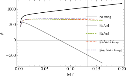
Previous phenomenological waveform constructions have dealt with this ambiguity by defining a standard form of the phase function by subtracting a fit to a linear function $\phi_{0}+\omega\,t_{0}$ over some suitably chosen frequency interval. In Fig. 16, phase functions after removing different fits to $\phi_{0}+\omega\,t_{0}$ are shown, and the ringdown frequency $f_{\text{RD}}$ is marked. The strong dependence of the phase function on the alignment and the fact that no particular features are visible at the ringdown makes it difficult to learn about qualitative features of the phase, in particular in the merger-ringdown regime.

Figure 16: Fourier domain phase corresponding to a hybrid constructed for SXS NR data corresponding to equal mass data with equal spins of $\chi_{i}=0.98$, with a term $\phi_{0}+\omega\,t_{0}$ subtracted over a frequency range. The frequency ranges of the fits are indicated in the plot, where $Mf_{S}=0.0035$ is the start frequency of clean hybrid hybrid data, and $Mf_{MR}=0.018$ the frequency where we typically separate between inspiral and merger-ringdown.

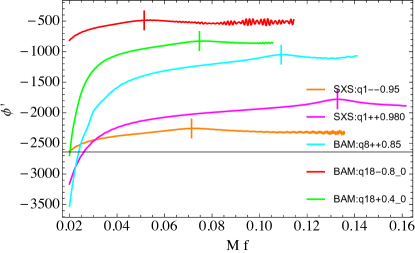
For this reason we take a different path to simplify the understanding of the anatomy of the phase functions, and we consider the first and second derivatives of the phase function with respect to the frequency. For NR data, the second derivative is often noisy and we thus mainly work with the first derivative, which eliminates the phase shift ambiguity and converts the time shift ambiguity into a simple constant offset. In Fig. 17 we plot the derivative of the phase for the same 5 “corner cases” of maximal mass ratio and/or spin shown in Fig. 6, and mark the ringdown frequency. We notice a characteristic structure rising above the background and centered at the ringdown frequency, which reminds us of the Lorentzian Eq. (28) we have previously employed to model the amplitude function. Taking a derivative of the Lorentzian, we can derive that the maxima of its derivative are located at $f_{RD}\pm f_{damp}/\sqrt{3}$. In Fig. 18 we compare this prediction for the second phase derivative with NR data from a BAM simulation, where we can compute a relatively clean second phase derivative, and we find excellent agreement. In order to capture the “background” in which the Lorentzian is embedded, we add terms with negative powers of the frequency $f$, to capture the steep inspiral gradient, and our basic model becomes,

$$\phi^{\prime}_{\text{MR}}=\alpha_{1}+\sum_{i=2}^{n}\alpha_{n}f^{-p_{n}}+\frac{a}{f_{damp}^{2}+(f-f_{RD})^{2}},$$ (34)

where the constant $\alpha_{0}$ acts as an overall time shift of the phase function, which could be determined by matching to a description of the inspiral, and the $\alpha_{i}$ and $a$ are free parameters which can be fit to numerical data. The number of free parameters $\alpha_{i}$ and the choice of powers $p_{n}$ defines a specific merger-ringdown ansatz. In order to find a good choice for the number of parameters and $p_{n}$, we first produce fits with the free parameters $(\alpha_{1},\alpha_{2},p_{2})$, and determine the best fit power $p_{n}$ across the parameter space. We find that $p_{2}\approx 2$, so we choose the integer $p_{2}=2$ as the leading contribution. Further terms can be added to the ansatz, e.g. until the residual across the parameter space resembles pure noise, and no further information can be extracted via fits. The specific choice made for the PhenomD model discussed in the companion paper is to add one more term with $p_{3}=-1/4$. In order to improve the convergence of Mathematica’s NonlinearModelFit function, we replace $f_{damp}$ by $\alpha_{0}f_{damp}$ in Eq. (34) and also fit to $\alpha_{0}$. We find that the parameter $\alpha_{0}$ is in the range $[0.98,1.04]$ and compensates for errors in our final mass and final spin fits near the boundary of our calibration region. For the actual PhenomD model discussed in Khan et al. (2015) this parameter will be set to unity.

For intermediate frequencies, roughly between $Mf=0.018$ and half the ringdown frequency one finds that the best choice of $p_{2}$ for a single power law coefficient in Eq.(34) is $p_{2}\approx 1$, so we choose the integer $p_{2}=1$ as the leading contribution in this regime, and we break up our model into different frequency ranges in each of which we use a very simple ansatz. A more sophisticated ansatz may successfully treat the entire frequency range with a single or at least only 2 fitting regions.

For consistency with our amplitude model, we again choose $Mf=0.018$ as the transition between our inspiral and high-frequency descriptions. For the merger-ringdown part, we find that a simple choice in terms of the ringdown frequency, e.g. $\left[0.45,1.15\right]f_{\text{RD}}$ is sufficient. The upper frequency $1.15f_{\text{RD}}$ approximates the highest frequency for which we have clean NR data. For the full IMR phase we use the above fit for frequencies larger than 0.5 $f_{\text{RD}}$.

For the intermediate phase we then choose a fitting window of $\left[0.018,0.6f_{\text{RD}}\right]$, and we use 2 fitting coefficients $p_{2}=1$, $p_{3}=4$.

Figure 17: Phase derivative $\phi^{\prime}$ for “corner cases” as indicated in the legend, vertical straight lines mark the ringdown frequency $f_{RD}$.

Figure 18: Second phase derivative for the BAM waveform with $q=2$, $\chi_{i}=0.75$, vertical straight lines mark the ringdown frequency $f_{RD}$ and $f_{RD}\pm f_{damp}/\sqrt{3}$.

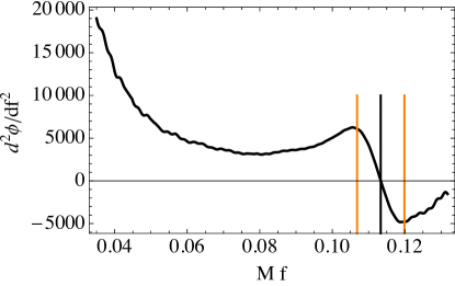
We thus have succeeded in directly using information about the final spin and mass in the ringdown description of both amplitude and phase, and turn now to using PN information for the inspiral. We can treat the inspiral along the lines of the amplitude in Sec.IV.1.1. For the amplitude we have added the next three higher order PN terms to the the known TaylorF2 expression. For the phase, the 4PN terms corresponds to a constant offset for the phase, to which we add the next three non-trivial higher order PN terms, thus four PN terms to be fitted in total.

V Summary

In this paper we have discussed preliminary work that will enable us to construct a new phenomenological waveform model for non-precessing waveforms in a companion paper Khan et al. (2015).

We have first presented new NR simulations which include data sets with a range of spin values at mass ratios 4, 8 and 18, which allow us to significantly extend the calibration range of current non-precessing inspiral-merger-ringdown models. We have demonstrated sixth order convergence for one of the $q=18$ cases and computed a phase error estimate on the order of $0.05$ radians after aligning near merger. We find in particular small secular drift, and errors that are dominated by noise and oscillations. We have illustrated high accuracy also for a $\sim$10 orbit aligned-spin case, where we have not completed the convergence series to save computational cost, and conclude that finite difference codes based on the “moving-puncture” paradigm Baker et al. (2006); Campanelli et al. (2006); Hannam et al. (2007b); Brügmann et al. (2008) provide a very robust tool to obtain NR data sets in new regions of parameter space.

We have then discussed our procedure to construct hybrid PN/numerical relativity waveforms in the time domain, and how to convert them to the frequency domain. Special emphasis has been put on the alignment procedure which is at the core of the hybridization procedure, and we have presented a comparison of our NR data and different PN approximants, from which we conclude that the most appropriate approximant to use in our hybrid construction is the uncalibrated SEOBv2 model. We have also described our simple criteria to determine an appropriate frequency range for the fitting procedure expressed in Eq. (10), which determines the optimal alignment of PN and NR waveforms. The PN comparison has been based on a time-shift analysis directly relevant to the hybridization procedure, which we have however also found very useful for other applications, such as studying the time-dependent dephasing of numerical simulations due to numerical error.

A crucial part of a waveform model is a prediction of the final mass and spin from the initial configuration, which then allows one to compute the complex quasi-normal ringdown frequencies. While there are a number of numerical fits to final mass and spin available in the literature Barausse and Rezzolla (2009); Hemberger et al. (2013b); Healy et al. (2014); Zlochower and Lousto (2015), we have presented new fits here, which extend the calibrated range, are particularly simple, and can easily be extended to new data sets or higher accuracy as further improvements of our waveform model are developed. An essential feature of the final spin fit for waveform modeling is that it respects the extreme Kerr limit. Also, the final state fits illustrate techniques for constructing parameter space fits which we will use in the companion paper Khan et al. (2015) to construct the PhenomD waveform model.

Previous phenomenological waveform models have used a Lorentzian to model the ringdown part of the Fourier amplitude, which however leads to an incorrect high frequency falloff behaviour ($f^{-2}$ instead of $O(f^{-M})\forall M$). Here we show that not only does a simple exponential factor lead to an excellent agreement with numerical data, but we also identify a Lorentzian of the same width, centered at the ringdown frequency in the derivative of the frequency domain phase.

For low frequencies, we model the amplitude and phase by the standard TaylorF2 approximant, augmented by pseudo-PN terms tuned to our hybrids constructed from SEOBv2 and NR data. For the amplitude, we use a re-expanded form with the imaginary part of the amplitude set to zero, i.e. we neglect the very small deviations between the GW phase and twice the orbital phase some of us discussed in Ref. Bustillo et al. (2015). We determine an appropriate cutoff frequency, where our inspiral model is separated from our merger ringdown model as $Mf=0.018$, considering the dependency of the inspiral amplitude fit residual on this cutoff frequency.

In order to model how the phase Lorentzian is embedded in the background functional dependance of the phase, we propose to complete the model by adding inverse powers of the frequency and identify the most appropriate leading term.

Having identified the Lorentzian feature in the phase, and a frequency up to which even a simple extension of the TaylorF2 approximant yields a good fit to the data, paves the way for complete waveform models of extremely high fidelity to the physical signal.

A first incarnation of our approach to develop phenomenological waveform models that are sufficiently accurate for the advanced detector era is the PhenomD model, which we present in a companion paper Khan et al. (2015).

References

- Khan et al. (2015) S. Khan, S. Husa, M. Hannam, F. Ohme, M. Pürrer, F. Jiménez Forteza, and A. Bohé (2015).
- Blanchet (2014) L. Blanchet, Living Reviews in Relativity 17 (2014), ISSN 1433-8351, URL http://dx.doi.org/10.12942/lrr-2014-2.
- Ajith (2008) P. Ajith, Class. Quant. Grav. 25, 114033 (2008), eprint 0712.0343.
- Buonanno et al. (2009) A. Buonanno, B. R. Iyer, E. Ochsner, Y. Pan, and B. S. Sathyaprakash, Phys. Rev. D 80 (2009), ISSN 1550-2368, URL http://dx.doi.org/10.1103/PhysRevD.80.084043.
- The LIGO Scientific Collaboration (2015) The LIGO Scientific Collaboration, LALSuite: LSC Algorithm Library Suite, https://www.lsc-group.phys.uwm.edu/daswg/projects/lalsuite.html (2015).
- Taracchini et al. (2014) A. Taracchini, A. Buonanno, Y. Pan, T. Hinderer, M. Boyle, D. A. Hemberger, L. E. Kidder, G. Lovelace, A. H. Mroué, H. P. Pfeiffer, et al., Phys. Rev. D 89 (2014), ISSN 1550-2368, URL http://dx.doi.org/10.1103/PhysRevD.89.061502.
- Aasi et al. (2013) J. Aasi et al. (LIGO Scientific Collaboration, Virgo Collaboration) (2013), eprint 1304.0670.
- Abadie et al. (2010) J. Abadie et al. (VIRGO, LIGO Scientific), Class. Quant. Grav. 27, 173001 (2010), eprint 1003.2480.
- Abbott et al. (2009) B. Abbott et al. (LIGO Scientific Collaboration), Rept.Prog.Phys. 72, 076901 (2009), eprint 0711.3041.
- Harry and LIGO Scientific Collaboration (2010) G. M. Harry and LIGO Scientific Collaboration, Classical and Quantum Gravity 27, 084006 (2010).
- Shoemaker and the Advanced LIGO Team (2009) D. Shoemaker and the Advanced LIGO Team, LIGO-M060056 (2009).
- Accadia et al. (2011) T. Accadia, F. Acernese, F. Antonucci, P. Astone, G. Ballardin, et al., Class.Quant.Grav. 28, 114002 (2011).
- Pretorius (2005) F. Pretorius, Physical Review Letters 95 (2005), ISSN 1079-7114, URL http://dx.doi.org/10.1103/PhysRevLett.95.121101.
- Buonanno and Damour (1999) A. Buonanno and T. Damour, Phys. Rev. D59, 084006 (1999), eprint gr-qc/9811091.
- Buonanno and Damour (2000) A. Buonanno and T. Damour, Phys. Rev. D62, 064015 (2000), eprint gr-qc/0001013.
- Buonanno et al. (2007) A. Buonanno, Y. Pan, J. G. Baker, J. Centrella, B. J. Kelly, S. T. McWilliams, and J. R. van Meter, Phys. Rev. D76, 104049 (2007), eprint 0706.3732.
- Damour et al. (2008) T. Damour, A. Nagar, M. Hannam, S. Husa, and B. Bruegmann, Phys. Rev. D78, 044039 (2008), eprint 0803.3162.
- Pan et al. (2011) Y. Pan, A. Buonanno, M. Boyle, L. T. Buchman, L. E. Kidder, H. P. Pfeiffer, and M. A. Scheel, Phys. Rev. D84, 124052 (2011), eprint 1106.1021.
- Damour et al. (2013) T. Damour, A. Nagar, and S. Bernuzzi, Phys.Rev. D87, 084035 (2013), eprint 1212.4357.
- Nagar et al. (2015) A. Nagar, T. Damour, C. Reisswig, and D. Pollney (2015), eprint 1506.08457.
- Field et al. (2014) S. E. Field, C. R. Galley, J. S. Hesthaven, J. Kaye, and M. Tiglio, Phys.Rev. X4, 031006 (2014), eprint 1308.3565.
- Pürrer (2014) M. Pürrer, Class. Quantum Grav. 31, 195010 (2014), ISSN 1361-6382, URL http://dx.doi.org/10.1088/0264-9381/31/19/195010.
- Pürrer (in prep.) M. Pürrer (in prep.).
- Ajith et al. (2007) P. Ajith, S. Babak, Y. Chen, M. Hewitson, B. Krishnan, J. T. Whelan, B. Brügmann, P. Diener, J. Gonzalez, M. Hannam, et al., Class. Quantum Grav. 24, S689 (2007), ISSN 1361-6382, URL http://dx.doi.org/10.1088/0264-9381/24/19/S31.
- Ajith et al. (2008) P. Ajith et al., Phys. Rev. D77, 104017 (2008), [Erratum: Phys. Rev.D79,129901(2009)], eprint 0710.2335.
- Ajith et al. (2011) P. Ajith, M. Hannam, S. Husa, Y. Chen, B. Brügmann, N. Dorband, D. Müller, F. Ohme, D. Pollney, C. Reisswig, et al., Physical Review Letters 106 (2011), ISSN 1079-7114, URL http://dx.doi.org/10.1103/PhysRevLett.106.241101.
- Santamaría et al. (2010) L. Santamaría, F. Ohme, P. Ajith, B. Brügmann, N. Dorband, M. Hannam, S. Husa, P. Mösta, D. Pollney, C. Reisswig, et al., Phys. Rev. D 82 (2010), ISSN 1550-2368, URL http://dx.doi.org/10.1103/PhysRevD.82.064016.
- Hannam et al. (2014) M. Hannam, P. Schmidt, A. Bohé, L. Haegel, S. Husa, et al., Phys.Rev.Lett. 113, 151101 (2014), eprint 1308.3271.
- Trefethen, Lloyd N. (1996) Trefethen, Lloyd N., Finite Difference and Spectral Methods for Ordinary and Partial Differential Equations (1996).
- (30) http://www.black-holes.org/waveforms.
- Ossokine et al. (2013) S. Ossokine, L. E. Kidder, and H. P. Pfeiffer, Phys.Rev. D88, 084031 (2013), eprint 1304.3067.
- Hemberger et al. (2013a) D. A. Hemberger, M. A. Scheel, L. E. Kidder, B. Szilagyi, G. Lovelace, et al., Class.Quant.Grav. 30, 115001 (2013a), eprint 1211.6079.
- Szilagyi et al. (2009) B. Szilagyi, L. Lindblom, and M. A. Scheel, Phys.Rev. D80, 124010 (2009), eprint 0909.3557.
- Scheel et al. (2009) M. A. Scheel, M. Boyle, T. Chu, L. E. Kidder, K. D. Matthews, et al., Phys.Rev. D79, 024003 (2009), eprint 0810.1767.
- Boyle et al. (2007) M. Boyle, D. A. Brown, L. E. Kidder, A. H. Mroué, H. P. Pfeiffer, et al., Phys.Rev. D76, 124038 (2007), eprint 0710.0158.
- Mroué et al. (2013) A. H. Mroué, M. A. Scheel, B. Szilagyi, H. P. Pfeiffer, M. Boyle, et al., Phys.Rev.Lett. 111, 241104 (2013), eprint 1304.6077.
- Buchman et al. (2012) L. T. Buchman, H. P. Pfeiffer, M. A. Scheel, and B. Szilagyi, Phys.Rev. D86, 084033 (2012), eprint 1206.3015.
- Brügmann et al. (2008) B. Brügmann, J. A. González, M. Hannam, S. Husa, U. Sperhake, and W. Tichy, Phys. Rev. D 77 (2008), ISSN 1550-2368, URL http://dx.doi.org/10.1103/PhysRevD.77.024027.
- Husa et al. (2008) S. Husa, J. A. González, M. Hannam, B. Brügmann, and U. Sperhake, Class. Quantum Grav. 25, 105006 (2008), ISSN 1361-6382, URL http://dx.doi.org/10.1088/0264-9381/25/10/105006.
- Scheel et al. (2014) M. A. Scheel, M. Giesler, D. A. Hemberger, G. Lovelace, K. Kuper, M. Boyle, B. Szilágyi, and L. E. Kidder (2014), eprint 1412.1803.
- Szilágyi (2014) B. Szilágyi, International Journal of Modern Physics D 23, 1430014 (2014), ISSN 1793-6594, URL http://dx.doi.org/10.1142/S0218271814300146.
- Szilágyi et al. (2015) B. Szilágyi, J. Blackman, A. Buonanno, A. Taracchini, H. P. Pfeiffer, M. A. Scheel, T. Chu, L. E. Kidder, and Y. Pan, Phys. Rev. Lett. 115, 031102 (2015), eprint 1502.04953.
- Cook and York (1990) G. B. Cook and J. York, James W., Phys.Rev. D41, 1077 (1990).
- Lovelace et al. (2008) G. Lovelace, R. Owen, H. P. Pfeiffer, and T. Chu, Phys.Rev. D78, 084017 (2008), eprint 0805.4192.
- Hannam et al. (2009a) M. Hannam, S. Husa, and N. O. Murchadha, Phys.Rev. D80, 124007 (2009a), eprint 0908.1063.
- Hannam et al. (2007a) M. Hannam, S. Husa, B. Bruegmann, J. A. Gonzalez, and U. Sperhake, Class.Quant.Grav. 24, S15 (2007a), eprint gr-qc/0612001.
- Ruchlin et al. (2014) I. Ruchlin, J. Healy, C. O. Lousto, and Y. Zlochower (2014), eprint 1410.8607.
- Lovelace et al. (2012) G. Lovelace, M. Boyle, M. A. Scheel, and B. Szilagyi, Class.Quant.Grav. 29, 045003 (2012), eprint 1110.2229.
- Boyle and Mroue (2009) M. Boyle and A. H. Mroue, Phys. Rev. D80, 124045 (2009), eprint 0905.3177.
- Shibata and Nakamura (1995) M. Shibata and T. Nakamura, Phys. Rev. D 52, 5428 (1995), URL http://link.aps.org/doi/10.1103/PhysRevD.52.5428.
- Baumgarte and Shapiro (1998) T. W. Baumgarte and S. L. Shapiro, Phys. Rev. D 59, 024007 (1998), URL http://link.aps.org/doi/10.1103/PhysRevD.59.024007.
- Brandt and Brügmann (1997) S. Brandt and B. Brügmann, Physical Review Letters 78, 3606 (1997), ISSN 1079-7114, URL http://dx.doi.org/10.1103/PhysRevLett.78.3606.
- Bowen and York (1980) J. Bowen and J. York, Phys. Rev. D 21, 2047 (1980), ISSN 0556-2821, URL http://dx.doi.org/10.1103/PhysRevD.21.2047.
- Ansorg et al. (2004) M. Ansorg, B. Brügmann, and W. Tichy, Phys. Rev. D 70 (2004), ISSN 1550-2368, URL http://dx.doi.org/10.1103/PhysRevD.70.064011.
- Lousto et al. (2010) C. O. Lousto, H. Nakano, Y. Zlochower, and M. Campanelli, Phys.Rev. D82, 104057 (2010), eprint 1008.4360.
- Nakano et al. (2011) H. Nakano, Y. Zlochower, C. O. Lousto, and M. Campanelli, Phys. Rev. D 84 (2011), ISSN 1550-2368, URL http://dx.doi.org/10.1103/PhysRevD.84.124006.
- Pürrer et al. (2012) M. Pürrer, S. Husa, and M. Hannam, Phys. Rev. D 85 (2012), ISSN 1550-2368, URL http://dx.doi.org/10.1103/PhysRevD.85.124051.
- Hannam et al. (2010a) M. Hannam, S. Husa, F. Ohme, and P. Ajith, Phys.Rev. D82, 124052 (2010a), eprint 1008.2961.
- Ohme et al. (2011) F. Ohme, M. Hannam, and S. Husa, Phys.Rev. D84, 064029 (2011), eprint 1107.0996.
- MacDonald et al. (2011) I. MacDonald, S. Nissanke, and H. P. Pfeiffer, Class. Quant. Grav. 28, 134002 (2011), eprint 1102.5128.
- MacDonald et al. (2013) I. MacDonald, A. H. Mroué, H. P. Pfeiffer, M. Boyle, L. E. Kidder, et al., Phys.Rev. D87, 024009 (2013), eprint 1210.3007.
- Damour et al. (2011) T. Damour, A. Nagar, and M. Trias, Phys. Rev. D83, 024006 (2011), eprint 1009.5998.
- Boyle (2011) M. Boyle, Phys. Rev. D84, 064013 (2011), eprint 1103.5088.
- Boyle et al. (2008) M. Boyle, A. Buonanno, L. E. Kidder, A. H. Mroue, Y. Pan, H. P. Pfeiffer, and M. A. Scheel, Phys. Rev. D78, 104020 (2008), eprint 0804.4184.
- Kumar et al. (2015) P. Kumar, K. Barkett, S. Bhagwat, N. Afshari, D. A. Brown, G. Lovelace, M. A. Scheel, and B. Szilágyi (2015), eprint 1507.00103.
- Hannam et al. (2010b) M. Hannam, S. Husa, F. Ohme, D. Muller, and B. Bruegmann, Phys. Rev. D82, 124008 (2010b), eprint 1007.4789.
- Kreiss, Heinz Otto and Oliger, Joseph (1977777773) Kreiss, Heinz Otto and Oliger, Joseph, Methods for the approximate solution of time dependent problems (1977777773).
- Hannam et al. (2009b) M. Hannam, S. Husa, J. G. Baker, M. Boyle, B. Bruegmann, et al., Phys.Rev. D79, 084025 (2009b), eprint 0901.2437.
- Ajith et al. (2012) P. Ajith, M. Boyle, D. A. Brown, B. Brügmann, L. T. Buchman, et al., Class.Quant.Grav. 29, 124001 (2012), eprint 1201.5319.
- Hinder et al. (2014) I. Hinder, A. Buonanno, M. Boyle, Z. B. Etienne, J. Healy, et al., Class.Quant.Grav. 31, 025012 (2014), eprint 1307.5307.
- Reisswig and Pollney (2011) C. Reisswig and D. Pollney, Class. Quant. Grav. 28, 195015 (2011), eprint 1006.1632.
- Bohé et al. (2013a) A. Bohé, S. Marsat, G. Faye, and L. Blanchet, Class.Quant.Grav. 30, 075017 (2013a), eprint 1212.5520.
- Bohé et al. (2013b) A. Bohé, S. Marsat, and L. Blanchet, Class.Quant.Grav. 30, 135009 (2013b), eprint 1303.7412.
- Bohé et al. (2015) A. Bohé, G. Faye, S. Marsat, and E. K. Porter (2015), eprint 1501.01529.
- Marsat (2015) S. Marsat, Class. Quant. Grav. 32, 085008 (2015), eprint 1411.4118.
- Taracchini et al. (2012) A. Taracchini, Y. Pan, A. Buonanno, E. Barausse, M. Boyle, T. Chu, G. Lovelace, H. P. Pfeiffer, and M. A. Scheel, Phys. Rev. D86, 024011 (2012), eprint 1202.0790.
- Bustillo et al. (2015) J. C. Bustillo, A. Bohé, S. Husa, A. M. Sintes, M. Hannam, and M. Pürrer (2015), eprint 1501.00918.
- Barausse and Rezzolla (2009) E. Barausse and L. Rezzolla, Astrophys. J. 704, L40 (2009), eprint 0904.2577.
- Hemberger et al. (2013b) D. A. Hemberger, G. Lovelace, T. J. Loredo, L. E. Kidder, M. A. Scheel, et al., Phys.Rev. D88, 064014 (2013b), eprint 1305.5991.
- Healy et al. (2014) J. Healy, C. O. Lousto, and Y. Zlochower, Phys. Rev. D90, 104004 (2014), eprint 1406.7295.
- Zlochower and Lousto (2015) Y. Zlochower and C. O. Lousto, Phys. Rev. D92, 024022 (2015), eprint 1503.07536.
- Berti et al. (2009) E. Berti, V. Cardoso, and A. O. Starinets, Class. Quant. Grav. 26, 163001 (2009), eprint 0905.2975.
- Berti, Emanuele and others (2015) Berti, Emanuele and others, Tables of kerr quasinormal frequencies (gravitational case: s=-2), http://www.phy.olemiss.edu/~berti/qnms.html (2015).
- Bardeen et al. (1972) J. M. Bardeen, W. H. Press, and S. A. Teukolsky, Astrophys. J. 178, 347 (1972).
- Pürrer et al. (2013) M. Pürrer, M. Hannam, P. Ajith, and S. Husa, Phys. Rev. D 88 (2013), ISSN 1550-2368, URL http://dx.doi.org/10.1103/PhysRevD.88.064007.
- Rezzolla et al. (2008) L. Rezzolla, P. Diener, E. N. Dorband, D. Pollney, C. Reisswig, E. Schnetter, and J. Seiler, Astrophys. J. 674, L29 (2008), eprint 0710.3345.
- Baker et al. (2006) J. G. Baker, J. Centrella, D.-I. Choi, M. Koppitz, and J. van Meter, Phys. Rev. Lett. 96, 111102 (2006), eprint gr-qc/0511103.
- Campanelli et al. (2006) M. Campanelli, C. O. Lousto, P. Marronetti, and Y. Zlochower, Phys. Rev. Lett. 96, 111101 (2006), eprint gr-qc/0511048.
- Hannam et al. (2007b) M. Hannam, S. Husa, D. Pollney, B. Bruegmann, and N. O’Murchadha, Phys. Rev. Lett. 99, 241102 (2007b), eprint gr-qc/0606099.