Dipole moments of charged leptons in the THDM-III with Textures

M. Arroyo-Ureña and Enrique Díaz Facultad de Ciencias Físico-Matemáticas
Benemérita Universidad Autónoma de Puebla, C.P. 72570, Puebla, Pue., Mexico.
(March 8, 2024)
Abstract

We study the magnetic and weak magnetic dipole moments of charged leptons in the framework of the Two Higgs Doublet Model type III (THDM-III) with four zero textures. We first analyze the possibility that the discrepancy between the experimental measurements and the theoretical prediction of the muon anomalous magnetic dipole moment (aμsubscript𝑎𝜇a_{\mu}) in the Standard Model (SM) can be explained in the context of the model and then find values for the parameters of the THDM-III: neutral and charged Higgs boson masses (mHsubscript𝑚𝐻m_{H}, mH±subscript𝑚superscript𝐻plus-or-minusm_{H^{\pm}}), mixing angles (α,β𝛼𝛽\alpha,{\beta}), CP-violating angles θ1,θ2subscript𝜃1subscript𝜃2\theta_{1},\,\theta_{2} and an additional parameter arising from the mass matrix (γfsubscript𝛾𝑓\gamma_{f}), for which a correspondence between theory and experiment is possible. We use aμTHDMIIIsuperscriptsubscript𝑎𝜇𝑇𝐻𝐷𝑀𝐼𝐼𝐼a_{\mu}^{THDM-III} and current low energy processes KK¯𝐾¯𝐾K-\bar{K} mixing, Bs0μμ¯superscriptsubscript𝐵𝑠0𝜇¯𝜇B_{s}^{0}\to\mu\bar{\mu}, τμμμ¯𝜏𝜇𝜇¯𝜇\tau\to\mu\mu\bar{\mu}, μeee¯𝜇𝑒𝑒¯𝑒\mu\to ee\bar{e}, τμγ𝜏𝜇𝛾\tau\to\mu\gamma, τeγ𝜏𝑒𝛾\tau\to e\gamma, μeγ𝜇𝑒𝛾\mu\to e\gamma, bsγ𝑏𝑠𝛾b\to s\gamma, BD(D)τν𝐵𝐷superscript𝐷𝜏𝜈B\to D(D^{*})\tau\nu and the rare higgs decay hτμ𝜏𝜇h\to\tau\mu in order to determine the allowed parameter space of THDM-III and from these we give a prediction for the magnetic and weak magnetic dipole moment of charged leptons, in particular of the τ𝜏\tau lepton. The obtained magnetic dipole moment of the τ𝜏\tau lepton is of the order of 𝒪(108107)𝒪superscript108superscript107\mathcal{O}(10^{-8}-10^{-7}) and the weak magnetic is of the order 𝒪(1010107)𝒪superscript1010superscript107\mathcal{O}(10^{-10}-10^{-7}).

pacs:
Valid PACS appear here
preprint: HEP-BUAP-01.13

I Introduction

The study of dipole moments in particle physics has become an important tool both theoretically and experimentally in the search of new physics. Motivated in part by the fact that within the SM the electric dipole moment at the one loop level is zero, albeit different Beyond the Standard Model (BSM) theories predict a small yet different than zero value, this would serve as a new source of CP violation. In regard to the magnetic dipole moments, the theoretical prediction of the aμsubscript𝑎𝜇a_{\mu} has been found to differ from the experimental value by [1]

Δaμ=aμExpaμSM=288(63)(49)×1011,Δsubscript𝑎𝜇superscriptsubscript𝑎𝜇𝐸𝑥𝑝superscriptsubscript𝑎𝜇𝑆𝑀2886349superscript1011\displaystyle\Delta a_{\mu}=a_{\mu}^{Exp}-a_{\mu}^{SM}=288(63)(49)\times 10^{-11}, (1)

which is greater than 3 standard deviations. This discrepancy between theory and experiment could give a hint to new physics. Of the several BSM models that have been used to try and offer a possible explanation to ΔaμΔsubscript𝑎𝜇\Delta a_{\mu}, one of the simplest is the THDM, as was done in the work of [2] and [3], which focused on THDM’s of the type I and type II. What differentiates each version of THDM is the way in which the Higgs doublets couple to fermions; in the type I only one of the doublets couples to all fermions while the other remains inert, type II has one doublet coupling exclusively to the up type quarks while the second doublet couples to down type quarks and leptons. Finally, in the type III (THDM-III) both doublets couple to all fermions, up and down quarks and leptons. As far as the authors know, no one has determined if the THDM-III is a viable model to explain ΔaμΔsubscript𝑎𝜇\Delta a_{\mu} and in turn how it might constrain the parameter space of the model.

Unlike the μ𝜇\mu, the τ𝜏\tau lepton has a short life-time of (290.3±0.5)×1015splus-or-minus290.30.5superscript1015𝑠(290{.}3\pm 0{.}5)\times 10^{-15}s that does not allow measurement of its anomalous moments by the spin precession method used with the electron and muon. The dipole moment of the τ𝜏\tau, with a 95% C.L., is [4]

0.052<aτ<0.013,0.052subscript𝑎𝜏0.013-0{.}052<a_{\tau}<0{.}013, (2)

with a central value

aτ=0.018(17),subscript𝑎𝜏0.01817a_{\tau}=-0{.}018(17), (3)

and the SM theoretical value is given by [5]

aτSM=1177.21(5)×106,superscriptsubscript𝑎𝜏𝑆𝑀1177.215superscript106a_{\tau}^{SM}=1177{.}21(5)\times 10^{-6}, (4)

different BSM models give predictions for the magnetic moment of the τ𝜏\tau between the range of 109superscript10910^{-9} to 106superscript10610^{-6} [6],[7],[8].

On the other hand, with respect to the weak properties of the τ𝜏\tau, the prediction of the SM was calculated in [9] whose value was found to be:

aτWSM=(2.10+0.61i)×106,superscriptsubscript𝑎𝜏𝑊𝑆𝑀2.100.61𝑖superscript106a_{\tau}^{W-SM}=-(2{.}10+0{.}61i)\times 10^{-6}, (5)

different BSM models predict values between the range of 1010superscript101010^{-10} to 106superscript10610^{-6} [6],[8],[10]. The real and imaginary part of the Weak Magnetic Dipole Moment (WMDM) of the τ𝜏\tau, with a 95% C.L., were reported in [11] and are given by

Re(aτW)<1.14×10³,Im(aτW)<2.65×10³,formulae-sequence𝑅𝑒superscriptsubscript𝑎𝜏𝑊1.14superscript103𝐼𝑚superscriptsubscript𝑎𝜏𝑊2.65superscript103Re\left(a_{\tau}^{W}\right)<1{.}14\times 10^{-3},\,Im\left(a_{\tau}^{W}\right)<2{.}65\times 10^{-3}, (6)

while the Weak Electric Dipole Moment (WEDM) is

Re(dτW)<0.5×10¹⁷ecm,Im(dτW)<1.1×10¹⁷ecm.formulae-sequence𝑅𝑒superscriptsubscript𝑑𝜏𝑊0.5superscript1017𝑒𝑐𝑚𝐼𝑚superscriptsubscript𝑑𝜏𝑊1.1superscript1017𝑒𝑐𝑚Re\left(d_{\tau}^{W}\right)<0{.}5\times 10^{-17}ecm,\,Im\left(d_{\tau}^{W}\right)<1{.}1\times 10^{-17}ecm. (7)

The f¯fV¯𝑓𝑓𝑉\overline{f}fV effective vertex describing the interaction between a neutral vector boson and two on–shell fermions can be written as:

ΓμffV(q2)=ie[γμ(FVVFVVγ5)qμ(iFSV+FPVγ5)+σμνqν(iFMV+FEVγ5)],superscriptsubscriptΓ𝜇𝑓𝑓𝑉superscript𝑞2𝑖𝑒delimited-[]subscript𝛾𝜇superscriptsubscript𝐹𝑉𝑉superscriptsubscript𝐹𝑉𝑉subscript𝛾5subscript𝑞𝜇𝑖superscriptsubscript𝐹𝑆𝑉superscriptsubscript𝐹𝑃𝑉subscript𝛾5subscript𝜎𝜇𝜈superscript𝑞𝜈𝑖superscriptsubscript𝐹𝑀𝑉superscriptsubscript𝐹𝐸𝑉subscript𝛾5\Gamma_{\mu}^{ffV}(q^{2})=ie\left[\gamma_{\mu}\left(F_{V}^{V}-F_{V}^{V}\gamma_{5}\right)-q_{\mu}\left(iF_{S}^{V}+F_{P}^{V}\gamma_{5}\right)+\sigma_{\mu\nu}q^{\nu}\left(iF_{M}^{V}+F_{E}^{V}\gamma_{5}\right)\right], (8)

where q=p2p1𝑞subscript𝑝2subscript𝑝1q=p_{2}-p_{1} is the four-momentum. The dipole moments are defined as follows:

af=2mfFMV=γ(0),df=eFEV=γ(0),formulae-sequencesubscript𝑎𝑓2subscript𝑚𝑓superscriptsubscript𝐹𝑀𝑉𝛾0subscript𝑑𝑓𝑒superscriptsubscript𝐹𝐸𝑉𝛾0a_{f}=-2m_{f}F_{M}^{V=\gamma}(0),\,d_{f}=-eF_{E}^{V=\gamma}(0), (9)

and the weak dipole moments

afW=2mfFMV=Z(mZ2),dfW=eFEV=Z(mZ2).formulae-sequencesuperscriptsubscript𝑎𝑓𝑊2subscript𝑚𝑓superscriptsubscript𝐹𝑀𝑉𝑍superscriptsubscript𝑚𝑍2superscriptsubscript𝑑𝑓𝑊𝑒superscriptsubscript𝐹𝐸𝑉𝑍superscriptsubscript𝑚𝑍2a_{f}^{W}=-2m_{f}F_{M}^{V=Z}(m_{Z}^{2}),d_{f}^{W}=-eF_{E}^{V=Z}(m_{Z}^{2}). (10)

In this work, we focus on the contributions to magnetic and weak magnetic dipole moments of charged leptons that arise from a THDM-III with a four zero texture. In particular we study the anomalous magnetic dipole moment of the τ𝜏\tau which can be measured through the decay τłντνl¯γsuperscript𝜏superscriptitalic-łsubscript𝜈𝜏¯subscript𝜈𝑙𝛾\tau^{-}\rightarrow\l^{-}\nu_{\tau}\overline{\nu_{l}}\gamma [12] and its weak magnetic dipole moment [13].

The structure of the paper is as follows; in section II we introduce the Lagrangian for the Yukawa sector of the THDM-III and how it can be expressed within the four zero texture framework. Afterwards in section III we present our calculations for the electromagnetic and weak dipole moments along with there one loop Feynman diagrams. While in section IV we present the effective Hamiltonians and the current values on experimental bounds and measurements for the Low energy processes considered. Results and numerical analysis are given in section V. Finally, our conclusions are presented in section VI.

II The Two Higgs Doublet Model with a Four Zero Texture

In this section we obtain the coupling of the Higgs bosons to fermions H(H±)fif¯j𝐻superscript𝐻plus-or-minussubscript𝑓𝑖subscript¯𝑓𝑗H(H^{\pm})f_{i}\overline{f}_{j}. We show the way in which we diagonalize the fermion mass matrix, where the structure of the Yukawa matrices is such that after summing them we recover a mass matrix with a 4 zero texture.

The general THDM, has been studied under different theoretical frameworks, such as the Minimal Flavor violating (MFV) THDM [14], which provides the minimal level of FCNC consistent with data. The THDM with Alignment is a scenario in which flavor violation does not occur at tree level; the contributions coming from vertices where flavor change occurs are not present and therefore could be smaller then the ones present in our model.

The assumption of textures implies a specific pattern of FCNC Higgs-fermion couplings, known as the Cheng-Sher ansatz mimjvsubscript𝑚𝑖subscript𝑚𝑗𝑣\frac{\sqrt{m_{i}m_{j}}}{v}. These vertices satisfy FCNC bounds for Higgs masses lighter than O(TeV), which is one of the reasons why we work in this formalism. Secondly, it gives the structure of the Yukawa matrices as a function of fermion masses in such a way that the elements of the CKM matrix are reproduced. But there are different possibilities for the texture forms, such as a textured six, five or four zero mass matrix which are ideas that has been extensively developed; one of the first efforts to work in this scheme assumed a six zero texture type [15], nonetheless this texture has been ruled out[16]. In this work we focus on the four zero type motivated by the fact that they currently satisfy many phenomenological observations. Furthermore, for certain four zero texture types as the Nearest Neighbor Interaction (NNI) is obtained through a Z4subscript𝑍4Z_{4} flavor symmetry in [17]. For a more in depth study of the formalism of textures and the THDM, we suggest Refs. [18], [19], [20].

The Yukawa Lagrangian of the THDM-III given by:

Yfsuperscriptsubscript𝑌𝑓\displaystyle\mathcal{L}_{Y}^{f} =\displaystyle= Y1uQ¯LΦ~1uR+Y2uQ¯LΦ~2uRsuperscriptsubscript𝑌1𝑢subscript¯𝑄𝐿subscript~Φ1subscript𝑢𝑅superscriptsubscript𝑌2𝑢subscript¯𝑄𝐿subscript~Φ2subscript𝑢𝑅\displaystyle Y_{1}^{u}\overline{Q}_{L}\tilde{\Phi}_{1}u_{R}+Y_{2}^{u}\overline{Q}_{L}\tilde{\Phi}_{2}u_{R}
+\displaystyle+ Y1dQ¯LΦ1dR+Y2dQ¯LΦ2dRsuperscriptsubscript𝑌1𝑑subscript¯𝑄𝐿subscriptΦ1subscript𝑑𝑅superscriptsubscript𝑌2𝑑subscript¯𝑄𝐿subscriptΦ2subscript𝑑𝑅\displaystyle Y_{1}^{d}\overline{Q}_{L}\Phi_{1}d_{R}+Y_{2}^{d}\overline{Q}_{L}\Phi_{2}d_{R}
+\displaystyle+ Y1lL¯LΦ1lR+Y2lL¯LΦ2lR+h.c.,formulae-sequencesuperscriptsubscript𝑌1𝑙subscript¯𝐿𝐿subscriptΦ1subscript𝑙𝑅superscriptsubscript𝑌2𝑙subscript¯𝐿𝐿subscriptΦ2subscript𝑙𝑅𝑐\displaystyle Y_{1}^{l}\overline{L}_{L}\Phi_{1}l_{R}+Y_{2}^{l}\overline{L}_{L}\Phi_{2}l_{R}+h.c.,

here Φi=(ϕi+,ϕi0)TsubscriptΦ𝑖superscriptsuperscriptsubscriptitalic-ϕ𝑖superscriptsubscriptitalic-ϕ𝑖0𝑇\Phi_{i}=(\phi_{i}^{+},\,\phi_{i}^{0})^{T} denote the Higgs doublets, Yifsuperscriptsubscript𝑌𝑖𝑓Y_{i}^{f} (f=u,d,l𝑓𝑢𝑑𝑙f=u,d,l) are 3×\times3 Yukawa matrices, Φ~j=iσ2Φjsubscript~Φ𝑗𝑖subscript𝜎2superscriptsubscriptΦ𝑗\tilde{\Phi}_{j}=i\sigma_{2}\Phi_{j}^{*} and Q¯L=(u¯L,d¯L)subscript¯𝑄𝐿subscript¯𝑢𝐿subscript¯𝑑𝐿\overline{Q}_{L}=(\bar{u}_{L},\,\bar{d}_{L}). Since both Higgs doublets couple to all fermions, the mass matrix for each fermion type f𝑓f receives contributions from both vevs v1subscript𝑣1v_{1} and v2subscript𝑣2v_{2}, i.e.

Mf=12(v1Y1f+v2Y2f).subscript𝑀𝑓12subscript𝑣1subscriptsuperscript𝑌𝑓1subscript𝑣2subscriptsuperscript𝑌𝑓2{M_{f}}=\frac{1}{\sqrt{2}}\left(v_{1}{Y}^{f}_{1}+v_{2}{Y}^{f}_{2}\right). (12)

In order to obtain physical fermion masses, we need to diagonalize the mass matrix; this is achieved through a bi-unitary transformation which is given by:

MD=𝒰fMf𝒰f=𝒰f12(v1Y1f+v2Y2f)𝒰f,subscript𝑀𝐷subscript𝒰𝑓subscript𝑀𝑓superscriptsubscript𝒰𝑓subscript𝒰𝑓12subscript𝑣1subscriptsuperscript𝑌𝑓1subscript𝑣2subscriptsuperscript𝑌𝑓2superscriptsubscript𝒰𝑓{M_{D}}=\mathcal{U}_{f}{M_{f}}\mathcal{U}_{f}^{\dagger}=\mathcal{U}_{f}\frac{1}{\sqrt{2}}\left(v_{1}{Y}^{f}_{1}+v_{2}{Y}^{f}_{2}\right)\mathcal{U}_{f}^{\dagger}, (13)

where the diagonalization matrix that we are using is obtained from [21]

𝒰f=𝒪fPf,subscript𝒰𝑓superscriptsubscript𝒪𝑓subscript𝑃𝑓\displaystyle\mathcal{U}_{f}=\mathcal{O}_{f}^{\dagger}P_{f}, (14)

in which 𝒪fsubscript𝒪𝑓\mathcal{O}_{f} is of the form

𝒪f=(m2m3(Am1)A(m2m1)(m3m1)m1m3(m2A)A(m2m1)(m3m2)m1m2(Am3)A(m3m1)(m3m2)m1(m1A)(m2m1)(m3m1)m2(Am2)(m2m1)(m3m2)m3(m3A)(m3m1)(m3m2)m1(Am2)(Am3)A(m2m1)(m3m1)m2(Am1)(m3A)A(m2m1)(m3m2)m3(Am1)(Am2)A(m3m1)(m3m2)),subscript𝒪𝑓subscript𝑚2subscript𝑚3𝐴subscript𝑚1𝐴subscript𝑚2subscript𝑚1subscript𝑚3subscript𝑚1subscript𝑚1subscript𝑚3subscript𝑚2𝐴𝐴𝑚2subscript𝑚1subscript𝑚3subscript𝑚2subscript𝑚1subscript𝑚2𝐴subscript𝑚3𝐴subscript𝑚3subscript𝑚1subscript𝑚3subscript𝑚2subscript𝑚1subscript𝑚1𝐴subscript𝑚2subscript𝑚1subscript𝑚3subscript𝑚1subscript𝑚2𝐴subscript𝑚2subscript𝑚2subscript𝑚1subscript𝑚3subscript𝑚2subscript𝑚3subscript𝑚3𝐴subscript𝑚3subscript𝑚1subscript𝑚3subscript𝑚2subscript𝑚1𝐴subscript𝑚2𝐴subscript𝑚3𝐴subscript𝑚2subscript𝑚1subscript𝑚3subscript𝑚1subscript𝑚2𝐴subscript𝑚1subscript𝑚3𝐴𝐴subscript𝑚2subscript𝑚1subscript𝑚3subscript𝑚2subscript𝑚3𝐴subscript𝑚1𝐴subscript𝑚2𝐴subscript𝑚3subscript𝑚1subscript𝑚3subscript𝑚2\displaystyle\small\mathcal{O}_{f}=\left(\begin{array}[]{ccc}\sqrt{\frac{m_{2}m_{3}(A-m_{1})}{A(m_{2}-m_{1})(m_{3}-m_{1})}}&\sqrt{\frac{m_{1}m_{3}(m_{2}-A)}{A(m2-m_{1})(m_{3}-m_{2})}}&\sqrt{\frac{m_{1}m_{2}(A-m_{3})}{A(m_{3}-m_{1})(m_{3}-m_{2})}}\\ -\sqrt{\frac{m_{1}(m_{1}-A)}{(m_{2}-m_{1})(m_{3}-m_{1})}}&\sqrt{\frac{m_{2}(A-m_{2})}{(m_{2}-m_{1})(m_{3}-m_{2})}}&\sqrt{\frac{m_{3}(m_{3}-A)}{(m_{3}-m_{1})(m_{3}-m_{2})}}\\ \sqrt{\frac{m_{1}(A-m_{2})(A-m_{3})}{A(m_{2}-m_{1})(m_{3}-m_{1})}}&-\sqrt{\frac{m_{2}(A-m_{1})(m_{3}-A)}{A(m_{2}-m_{1})(m_{3}-m_{2})}}&\sqrt{\frac{m_{3}(A-m_{1})(A-m_{2})}{A(m_{3}-m_{1})(m_{3}-m_{2})}}\end{array}\right), (18)

such that A=m3(1γfr2)𝐴subscript𝑚31subscript𝛾𝑓subscript𝑟2A=m_{3}(1-\gamma_{f}r_{2}) with f=l,u,d𝑓𝑙𝑢𝑑f=l,\,u,\,d and r2=m2m3subscript𝑟2subscript𝑚2subscript𝑚3r_{2}=\frac{m_{2}}{m_{3}}, and

P=(1000eiθ1000eiθ2).𝑃1000superscript𝑒𝑖subscript𝜃1000superscript𝑒𝑖subscript𝜃2\displaystyle P=\left(\begin{array}[]{ccc}1&0&0\\ 0&e^{i\theta_{1}}&0\\ 0&0&e^{i\theta_{2}}\\ \end{array}\right). (22)

The neutral Yukawa Lagrangian given in Eq. (II) can be expressed in terms of the mass eigenstates h0superscript0h^{0}, H0superscript𝐻0H^{0}, A0superscript𝐴0A^{0} as [22]

Yneusuperscriptsubscript𝑌𝑛𝑒𝑢\displaystyle\mathcal{L}_{Y}^{neu} =\displaystyle= g2(mlmW)l¯[cosαcosβδll+2sin(αβ)gcosβ(mWml)(Y~2l)ll]lH0\displaystyle\frac{g}{2}\left(\frac{m_{l}}{m_{W}}\right)\bar{l}\left[\frac{\cos\alpha}{\cos\beta}\delta_{ll{{}^{\prime}}}+\frac{\sqrt{2}\sin(\alpha-\beta)}{g\cos\beta}\left(\frac{m_{W}}{m_{l}}\right)\left(\tilde{Y}_{2}^{l}\right)_{ll{{}^{\prime}}}\right]l{{}^{\prime}}H^{0}
+\displaystyle+ g2(mlmW)l¯[sinαcosβδll+2cos(αβ)gcosβ(mWml)(Y~2l)ll]lh0\displaystyle\frac{g}{2}\left(\frac{m_{l}}{m_{W}}\right)\bar{l}\left[-\frac{\sin\alpha}{\cos\beta}\delta_{ll{{}^{\prime}}}+\frac{\sqrt{2}\cos(\alpha-\beta)}{g\cos\beta}\left(\frac{m_{W}}{m_{l}}\right)\left(\tilde{Y}_{2}^{l}\right)_{ll{{}^{\prime}}}\right]l{{}^{\prime}}h^{0}
+\displaystyle+ ig2(mlmW)l¯[tanβδll+2gcosβ(mWml)(Y~2l)ll]γ5lA0\displaystyle\frac{ig}{2}\left(\frac{m_{l}}{m_{W}}\right)\bar{l}\left[-\tan\beta\delta_{ll{{}^{\prime}}}+\frac{\sqrt{2}}{g\cos\beta}\left(\frac{m_{W}}{m_{l}}\right)\left(\tilde{Y}_{2}^{l}\right)_{ll{{}^{\prime}}}\right]\gamma^{5}l{{}^{\prime}}A^{0}
+\displaystyle+ g2(mumW)u¯[sinαsinβδuu+2sin(αβ)gsinβ(mWmu)(Y~2l)uu]uH0\displaystyle\frac{g}{2}\left(\frac{m_{u}}{m_{W}}\right)\bar{u}\left[\frac{\sin\alpha}{\sin\beta}\delta_{uu{{}^{\prime}}}+\frac{\sqrt{2}\sin(\alpha-\beta)}{g\sin\beta}\left(\frac{m_{W}}{m_{u}}\right)\left(\tilde{Y}_{2}^{l}\right)_{uu{{}^{\prime}}}\right]u{{}^{\prime}}H^{0}
+\displaystyle+ g2(mumW)u¯[cosαsinβδuu+2cos(αβ)gsinβ(mWmu)(Y~2u)uu]uh0\displaystyle\frac{g}{2}\left(\frac{m_{u}}{m_{W}}\right)\bar{u}\left[-\frac{\cos\alpha}{\sin\beta}\delta_{uu{{}^{\prime}}}+\frac{\sqrt{2}\cos(\alpha-\beta)}{g\sin\beta}\left(\frac{m_{W}}{m_{u}}\right)\left(\tilde{Y}_{2}^{u}\right)_{uu{{}^{\prime}}}\right]u{{}^{\prime}}h^{0}
+\displaystyle+ ig2(mumW)u¯[cotβδuu+2gsinβ(mWmu)(Y~2u)uu]γ5uA0,\displaystyle\frac{ig}{2}\left(\frac{m_{u}}{m_{W}}\right)\bar{u}\left[-\cot\beta\delta_{uu{{}^{\prime}}}+\frac{\sqrt{2}}{g\sin\beta}\left(\frac{m_{W}}{m_{u}}\right)\left(\tilde{Y}_{2}^{u}\right)_{uu{{}^{\prime}}}\right]\gamma^{5}u{{}^{\prime}}A^{0},

where Y~2f=2v2MDv1v2Y~1fsuperscriptsubscript~𝑌2𝑓2subscript𝑣2subscript𝑀𝐷subscript𝑣1subscript𝑣2superscriptsubscript~𝑌1𝑓\tilde{Y}_{2}^{f}=\frac{\sqrt{2}}{v_{2}}M_{D}-\frac{v_{1}}{v_{2}}\tilde{Y}_{1}^{f} and Y~if=𝒰fYif𝒰fsuperscriptsubscript~𝑌𝑖𝑓subscript𝒰𝑓subscriptsuperscript𝑌𝑓𝑖superscriptsubscript𝒰𝑓\tilde{Y}_{i}^{f}=\mathcal{U}_{f}{Y}^{f}_{i}\mathcal{U}_{f}^{\dagger}. The type-down quarks part is similar to the lepton part with the exchange ld𝑙𝑑l\to d and mlmdsubscript𝑚𝑙subscript𝑚𝑑m_{l}\to m_{d}.

On the other hand, the charged Yukawa Lagrangian is given by:

Ychsuperscriptsubscript𝑌𝑐\displaystyle\mathcal{L}_{Y}^{ch} =\displaystyle= [d¯i(Y~1usinβ+Y~2ucosβ)ujH\displaystyle\left[\bar{d}_{i}\left(\tilde{Y}_{1}^{u}sin\beta+\tilde{Y}_{2}^{u}cos\beta\right)u_{j}H^{-}\right.
+\displaystyle+ u¯i(Y~2dcosβY~1dsinβ)djH+]PR\displaystyle\left.\bar{u}_{i}\left(\tilde{Y}_{2}^{d}cos\beta-\tilde{Y}_{1}^{d}sin\beta\right)d_{j}H^{+}\right]P_{R}
+\displaystyle+ [d¯i(Y~2ucosβY~1usinβ)ujH\displaystyle\left[\bar{d}_{i}\left(\tilde{Y}_{2}^{u}cos\beta-\tilde{Y}_{1}^{u}sin\beta\right)u_{j}H^{-}\right.
+\displaystyle+ u¯i(Y~1dsinβY~2dcosβ)djH+]PL.\displaystyle\left.\bar{u}_{i}\left(\tilde{Y}_{1}^{d}sin\beta-\tilde{Y}_{2}^{d}cos\beta\right)d_{j}H^{+}\right]P_{L}.

We will use a notation in which ηff¯Hsuperscriptsubscript𝜂𝑓¯𝑓𝐻\eta_{f\bar{f}}^{H} corresponds to the couplings ff¯H𝑓¯𝑓𝐻f\bar{f}H in the Lagrangians, for example:

ηll¯H0=g2(mlmW)[cosαcosβδll+2sin(αβ)gcosβ(mWml)(Y~2l)ll].\eta_{l\bar{l}}^{H^{0}}=\frac{g}{2}\left(\frac{m_{l}}{m_{W}}\right)\left[\frac{\cos\alpha}{\cos\beta}\delta_{ll{{}^{\prime}}}+\frac{\sqrt{2}\sin(\alpha-\beta)}{g\cos\beta}\left(\frac{m_{W}}{m_{l}}\right)\left(\tilde{Y}_{2}^{l}\right)_{ll{{}^{\prime}}}\right]. (25)

In this work, we assume that the mass matrix has a four zero texture form

Mf=(0Df0DfCfBf0BfAf),subscript𝑀𝑓0subscript𝐷𝑓0superscriptsubscript𝐷𝑓subscript𝐶𝑓subscript𝐵𝑓0superscriptsubscript𝐵𝑓subscript𝐴𝑓\displaystyle{M_{f}}=\left(\begin{array}[]{ccc}0&D_{f}&0\\ D_{f}^{*}&C_{f}&B_{f}\\ 0&B_{f}^{*}&A_{f}\end{array}\right), (29)

so

(0Df0DfCfBf0BfA)=v12(0d10d1c1b10b1a1)+v22(0d20d2c2b20b2a2),0subscript𝐷𝑓0superscriptsubscript𝐷𝑓subscript𝐶𝑓subscript𝐵𝑓0superscriptsubscript𝐵𝑓𝐴subscript𝑣120subscript𝑑10subscriptsuperscript𝑑1subscript𝑐1subscript𝑏10subscriptsuperscript𝑏1subscript𝑎1subscript𝑣220subscript𝑑20subscriptsuperscript𝑑2subscript𝑐2subscript𝑏20subscriptsuperscript𝑏2subscript𝑎2\displaystyle\left(\begin{array}[]{ccc}0&D_{f}&0\\ D_{f}^{*}&C_{f}&B_{f}\\ 0&B_{f}^{*}&A\end{array}\right)=\frac{v_{1}}{\sqrt{2}}\left(\begin{array}[]{ccc}0&d_{1}&0\\ d^{*}_{1}&c_{1}&b_{1}\\ 0&b^{*}_{1}&a_{1}\\ \end{array}\right)+\frac{v_{2}}{\sqrt{2}}\left(\begin{array}[]{ccc}0&d_{2}&0\\ d^{*}_{2}&c_{2}&b_{2}\\ 0&b^{*}_{2}&a_{2}\\ \end{array}\right), (39)

where

Yi=(0di0dicibi0biai),i=1, 2.formulae-sequencesubscript𝑌𝑖0subscript𝑑𝑖0superscriptsubscript𝑑𝑖subscript𝑐𝑖subscript𝑏𝑖0superscriptsubscript𝑏𝑖subscript𝑎𝑖𝑖12Y_{i}=\left(\begin{array}[]{ccc}0&d_{i}&0\\ d_{i}^{*}&c_{i}&b_{i}\\ 0&b_{i}^{*}&a_{i}\end{array}\right),\>i=1,\,2.

To find the expression for the mass eigenstates, we use the following matrix invariants:

Tr(Mf)𝑇𝑟subscript𝑀𝑓\displaystyle Tr(M_{f}) =\displaystyle= Cf+Af=mf3+mf2+mf1,subscript𝐶𝑓subscript𝐴𝑓subscript𝑚subscript𝑓3subscript𝑚subscript𝑓2subscript𝑚subscript𝑓1\displaystyle C_{f}+A_{f}=m_{f_{3}}+m_{f_{2}}+m_{f_{1}}, (40)
det(Mf)𝑑𝑒𝑡subscript𝑀𝑓\displaystyle det(M_{f}) =\displaystyle= Df2Af=mf1mf2mf3,superscriptsubscript𝐷𝑓2subscript𝐴𝑓subscript𝑚subscript𝑓1subscript𝑚subscript𝑓2subscript𝑚subscript𝑓3\displaystyle-D_{f}^{2}A_{f}=m_{f_{1}}m_{f_{2}}m_{f_{3}}, (41)
χ(Mf)𝜒subscript𝑀𝑓\displaystyle\chi(M_{f}) =\displaystyle= Bf2+CfAfDf2=mf1mf2+mf1mf3+mf2mf3,superscriptsubscript𝐵𝑓2subscript𝐶𝑓subscript𝐴𝑓superscriptsubscript𝐷𝑓2subscript𝑚subscript𝑓1subscript𝑚subscript𝑓2subscript𝑚subscript𝑓1subscript𝑚subscript𝑓3subscript𝑚subscript𝑓2subscript𝑚subscript𝑓3\displaystyle B_{f}^{2}+C_{f}A_{f}-D_{f}^{2}=m_{f_{1}}m_{f_{2}}+m_{f_{1}}m_{f_{3}}+m_{f_{2}}m_{f_{3}}, (42)

from these expressions we find a relation between the components of the 4-texture mass matrix and the physical fermion masses

Afsubscript𝐴𝑓\displaystyle A_{f} =\displaystyle= mf3(1r2γf),subscript𝑚subscript𝑓31subscript𝑟2subscript𝛾𝑓\displaystyle m_{f_{3}}\left(1-r_{2}\gamma_{f}\right), (43)
Bfsubscript𝐵𝑓\displaystyle B_{f} =\displaystyle= mf3r2γf(r2γf+r11)(r2γf+r21)1r2γf,subscript𝑚subscript𝑓3subscript𝑟2subscript𝛾𝑓subscript𝑟2subscript𝛾𝑓subscript𝑟11subscript𝑟2subscript𝛾𝑓subscript𝑟211subscript𝑟2subscript𝛾𝑓\displaystyle m_{f_{3}}\sqrt{\frac{r_{2}\gamma_{f}\left(r_{2}\gamma_{f}+r_{1}-1\right)\left(r_{2}\gamma_{f}+r_{2}-1\right)}{1-r_{2}\gamma_{f}}}, (44)
Cfsubscript𝐶𝑓\displaystyle C_{f} =\displaystyle= mf3(r2γf+r1+r2),subscript𝑚subscript𝑓3subscript𝑟2subscript𝛾𝑓subscript𝑟1subscript𝑟2\displaystyle m_{f_{3}}\left(r_{2}\gamma_{f}+r_{1}+r_{2}\right), (45)
Dfsubscript𝐷𝑓\displaystyle D_{f} =\displaystyle= mf1mf21r2γf,subscript𝑚subscript𝑓1subscript𝑚subscript𝑓21subscript𝑟2subscript𝛾𝑓\displaystyle\sqrt{-\frac{m_{f_{1}}m_{f_{2}}}{1-{r_{2}}\gamma_{f}}}, (46)

where mfisubscript𝑚subscript𝑓𝑖m_{f_{i}} is the fermion mass and the risubscript𝑟𝑖r_{i} stands for ri=mfimf3subscript𝑟𝑖subscript𝑚subscript𝑓𝑖subscript𝑚subscript𝑓3r_{i}=\frac{m_{f_{i}}}{m_{f_{3}}}.

So far, we have found a relation between the textured mass matrix and the diagonal physical mass matrix, but the coupling of fermions to the scalar is given through the Yukawas, whose elements a1,2subscript𝑎12a_{1,2}, b1,2subscript𝑏12b_{1,2}, c1,2subscript𝑐12c_{1,2} and d1,2subscript𝑑12d_{1,2} can not be simultaneously determined. But instead of having them as free parameters we can do the following:

Case 1) We will assume that the elements of Y1subscript𝑌1Y_{1} are negligible and so

Mf=(0Df0DfCfBf0BfA)v22(0d20d2c2b20b2a2).subscript𝑀𝑓0subscript𝐷𝑓0superscriptsubscript𝐷𝑓subscript𝐶𝑓subscript𝐵𝑓0superscriptsubscript𝐵𝑓𝐴subscript𝑣220subscript𝑑20subscriptsuperscript𝑑2subscript𝑐2subscript𝑏20subscriptsuperscript𝑏2subscript𝑎2\displaystyle M_{f}=\left(\begin{array}[]{ccc}0&D_{f}&0\\ D_{f}^{*}&C_{f}&B_{f}\\ 0&B_{f}^{*}&A\end{array}\right)\approx\frac{v_{2}}{\sqrt{2}}\left(\begin{array}[]{ccc}0&d_{2}&0\\ d^{*}_{2}&c_{2}&b_{2}\\ 0&b^{*}_{2}&a_{2}\\ \end{array}\right). (53)

Case 2a) Following [30], we will consider the case in which each Yukawa contributes to only one element of the mass matrix

Mf=(0Df0DfCfBf0BfA)=v12(0d10d1c1b10b10)+v22(00000000a2),subscript𝑀𝑓0subscript𝐷𝑓0superscriptsubscript𝐷𝑓subscript𝐶𝑓subscript𝐵𝑓0superscriptsubscript𝐵𝑓𝐴subscript𝑣120subscript𝑑10superscriptsubscript𝑑1subscript𝑐1subscript𝑏10superscriptsubscript𝑏10subscript𝑣2200000000subscript𝑎2\displaystyle M_{f}=\left(\begin{array}[]{ccc}0&D_{f}&0\\ D_{f}^{*}&C_{f}&B_{f}\\ 0&B_{f}^{*}&A\end{array}\right)=\frac{v_{1}}{\sqrt{2}}\left(\begin{array}[]{ccc}0&d_{1}&0\\ d_{1}^{*}&c_{1}&b_{1}\\ 0&b_{1}^{*}&0\\ \end{array}\right)+\frac{v_{2}}{\sqrt{2}}\left(\begin{array}[]{ccc}0&0&0\\ 0&0&0\\ 0&0&a_{2}\\ \end{array}\right), (63)

or

Case 2b)

Mf=(0Df0DfCfBf0BfA)=v12(0000c10000)+v22(0d20d20b20b2a2).subscript𝑀𝑓0subscript𝐷𝑓0superscriptsubscript𝐷𝑓subscript𝐶𝑓subscript𝐵𝑓0superscriptsubscript𝐵𝑓𝐴subscript𝑣120000subscript𝑐10000subscript𝑣220subscript𝑑20superscriptsubscript𝑑20subscript𝑏20superscriptsubscript𝑏2subscript𝑎2\displaystyle M_{f}=\left(\begin{array}[]{ccc}0&D_{f}&0\\ D_{f}^{*}&C_{f}&B_{f}\\ 0&B_{f}^{*}&A\end{array}\right)=\frac{v_{1}}{\sqrt{2}}\left(\begin{array}[]{ccc}0&0&0\\ 0&c_{1}&0\\ 0&0&0\\ \end{array}\right)+\frac{v_{2}}{\sqrt{2}}\left(\begin{array}[]{ccc}0&d_{2}&0\\ d_{2}^{*}&0&b_{2}\\ 0&b_{2}^{*}&a_{2}\\ \end{array}\right). (73)

in both cases, the structure of the Yukawa matrices textures is such that after summing both we recover a mass matrix with a 4 zero texture. In working under any of these assumptions we avoid introducing new free parameters instead of explicitly determining the Yukawa matrix elements as functions of the fermion masses and γfsubscript𝛾𝑓\gamma_{f}. The (Y~2)ffsubscriptsubscript~𝑌2𝑓superscript𝑓\left(\tilde{Y}_{2}\right)_{ff^{\prime}} for the paralell case is shown in the App.VII.1 and for cases 2a and 2b are given in [30].

In regard to the Renormalization Group Equations (RGE) stability, a study of the RGE in the general THDM-III has already been performed by the authors of [31], they found a remarkable stability of the suppressed FCNC Yukawa coupling parameters. Furthermore, in [32] they explored if four zero textures are stable under the running of energy scales and found that the texture zeros of mass matrices Mfsubscript𝑀𝑓M_{f} are stable against the evolution of energy scales.

III DIPOLE MOMENTS IN THE THDM-III with four zero texture

In this section we give our expressions for the magnetic and weak magnetic dipole moments of charged leptons within the THDM-III.

III.1 MUON ANOMALOUS MAGNETIC DIPOLE MOMENT

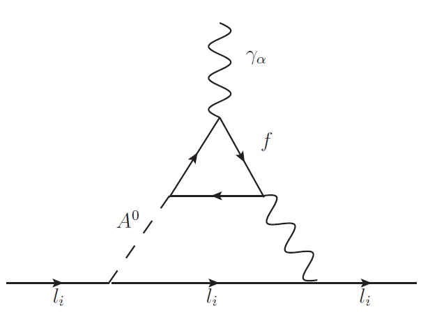
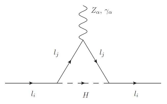
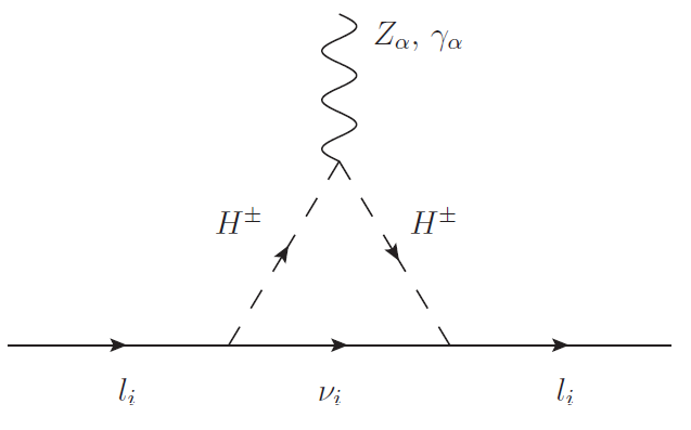
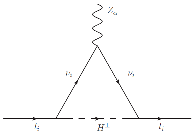
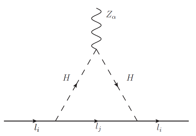
The Feynman diagrams that contribute to the magnetic dipole moment of charged leptons in the framework of the THDM-III are shown in FIG.[1],
Refer to caption
(a)
Refer to caption
(b)
Refer to caption
(c)
Figure 1: Feynman diagrams that contribute to the magnetic dipole moment of charged leptons in the framework of the THDM-III. In the case of the contributions coming of Barr-Zee diagrams we only consider the dominant contribution given by diagram (c).

where li=esubscript𝑙𝑖𝑒l_{i}=e, μ𝜇\mu, τ𝜏\tau, and ljsubscript𝑙𝑗l_{j} refers to a lepton of different flavor, H=h0,H0,A0𝐻superscript0superscript𝐻0superscript𝐴0H=h^{0},H^{0},A^{0} are the neutral light, heavy and pseudo scalar Higgs bosons, respectively. The vertices coupling Higgs bosons to charged fermions are obtained from the Lagrangian in eqs.(II-II), except for the vertices coupling Higgs bosons to gauge bosons and Z to neutrinos [23]. The contributions to the magnetic dipole moments of leptons are CP-conserving, therefore the phases θ1, 2subscript𝜃12\theta_{1,\,2} are set to zero.

We perform the calculation in the unitary gauge via the Feynman parameters. The one-loop contribution is given by:

aliρ1ρ2ρ3=l=1, 2, 3l=2|ηllρ1ρ2ρ3|2mli8π201𝑑x01x𝑑yGkρ1ρ2ρ3(x,y),superscriptsubscript𝑎subscript𝑙𝑖subscript𝜌1subscript𝜌2subscript𝜌3superscript𝑙2𝑙123superscriptsuperscriptsubscript𝜂𝑙superscript𝑙subscript𝜌1subscript𝜌2subscript𝜌32subscript𝑚subscript𝑙𝑖8superscript𝜋2superscriptsubscript01differential-d𝑥superscriptsubscript01𝑥differential-d𝑦superscriptsubscript𝐺𝑘subscript𝜌1subscript𝜌2subscript𝜌3𝑥𝑦a_{l_{i}}^{\rho_{1}\rho_{2}\rho_{3}}=\underset{\underset{l^{\prime}=2}{l=1,\,2,\,3}}{\sum}\frac{\left|\eta_{{}_{ll^{\prime}}}^{\rho_{1}\rho_{2}\rho_{3}}\right|^{2}m_{l_{i}}}{\sqrt{8}\pi^{2}}\intop_{0}^{1}dx\intop_{0}^{1-x}dy\,G_{k}^{\rho_{1}\rho_{2}\rho_{3}}(x,\,y), (74)

where the label ρnsubscript𝜌𝑛\rho_{n} refers to the particles circulating in each diagram, and the index ll𝑙superscript𝑙ll^{\prime} denotes the entry of the Yukawa interaction, in the case for the aμsubscript𝑎𝜇a_{\mu}: l=2superscript𝑙2l^{\prime}=2, i.e. l2𝑙2l2 with l=1, 2, 3𝑙123l=1,\,2,\,3. Notice that our results can be applied to any of the charged lepton. The label ηllρ1ρ2ρ3superscriptsubscript𝜂𝑙superscript𝑙subscript𝜌1subscript𝜌2subscript𝜌3\eta_{{}_{ll^{\prime}}}^{\rho_{1}\rho_{2}\rho_{3}} is the coupling obtained from the neutral Lagrangian term of ll¯H𝑙¯𝑙𝐻l\bar{l}H.

The Gkρ1ρ2ρ3(x,y)superscriptsubscript𝐺𝑘subscript𝜌1subscript𝜌2subscript𝜌3𝑥𝑦G_{k}^{\rho_{1}\rho_{2}\rho_{3}}(x,\,y) function for the diagram (a) is given by:

GaHljlj(x,y)=(x+y)(mljmli(x+y1))/Ma2,superscriptsubscript𝐺𝑎𝐻subscript𝑙𝑗subscript𝑙𝑗𝑥𝑦𝑥𝑦subscript𝑚subscript𝑙𝑗subscript𝑚subscript𝑙𝑖𝑥𝑦1superscriptsubscript𝑀𝑎2G_{a}^{{H}l_{j}l_{j}}(x,\,y)=(x+y)(m_{l_{j}}-m_{l_{i}}(x+y-1))/M_{a}^{2}, (75)

with Ma2=mH2(x+y1)+(x+y)(mlj2+mli2(x+y1)M_{a}^{2}=-m_{H}^{2}(x+y-1)+(x+y)(m_{l_{j}}^{2}+m_{l_{i}}^{2}(x+y-1). Here lj=e,μ,τ.subscript𝑙𝑗𝑒𝜇𝜏l_{j}=e,\,\mu,\,\tau. For the Feynman diagram (b): ηllρ1ρ2ρ3=1superscriptsubscript𝜂𝑙superscript𝑙subscript𝜌1subscript𝜌2subscript𝜌31\eta_{{}_{ll^{\prime}}}^{\rho_{1}\rho_{2}\rho_{3}}=1 and Gbρ1ρ2ρ3(x)superscriptsubscript𝐺𝑏subscript𝜌1subscript𝜌2subscript𝜌3𝑥G_{b}^{\rho_{1}\rho_{2}\rho_{3}}(x) function is given by:

GbH±H±ν(x)=2mlix/Mb2,superscriptsubscript𝐺𝑏superscript𝐻plus-or-minussuperscript𝐻plus-or-minus𝜈𝑥2subscript𝑚subscript𝑙𝑖𝑥superscriptsubscript𝑀𝑏2G_{b}^{H^{\pm}H^{\pm}\nu}(x)=2m_{l_{i}}x/M_{b}^{2}, (76)

with Mb2=(mli2xmH±2)superscriptsubscript𝑀𝑏2superscriptsubscript𝑚subscript𝑙𝑖2𝑥superscriptsubscript𝑚superscript𝐻plus-or-minus2M_{b}^{2}=(m_{l_{i}}^{2}x-m_{H^{\pm}}^{2}). The THDM also has Barr-Zee two-loop contributions to the muon anomalous magnetic moment. The dominant contribution is given by [24]

aμtwoloop=α28π2sW2mμ2ημμ¯A0mW2f=t,τ,bNcfQf2rff(rf)ηff¯A0,superscriptsubscript𝑎𝜇𝑡𝑤𝑜𝑙𝑜𝑜𝑝superscript𝛼28superscript𝜋2superscriptsubscript𝑠𝑊2superscriptsubscript𝑚𝜇2superscriptsubscript𝜂𝜇¯𝜇superscript𝐴0superscriptsubscript𝑚𝑊2subscript𝑓𝑡𝜏𝑏superscriptsubscript𝑁𝑐𝑓superscriptsubscript𝑄𝑓2subscript𝑟𝑓𝑓subscript𝑟𝑓superscriptsubscript𝜂𝑓¯𝑓superscript𝐴0a_{\mu}^{two\,loop}=\frac{\alpha^{2}}{8\pi^{2}s_{W}^{2}}\frac{m_{\mu}^{2}\eta_{\mu\bar{\mu}}^{A^{0}}}{m_{W}^{2}}\sum_{f=t,\,\tau,\,b}N_{c}^{f}Q_{f}^{2}r_{f}f(r_{f})\eta_{f\bar{f}}^{A^{0}}, (77)

where rf=(mf/mA0)subscript𝑟𝑓subscript𝑚𝑓superscriptsubscript𝑚𝐴0r_{f}=(m_{f}/m_{A}^{0}), mfsubscript𝑚𝑓m_{f} is the fermion mass, Ncf=1(3)superscriptsubscript𝑁𝑐𝑓13N_{c}^{f}=1(3) for leptons (quarks), Qfsubscript𝑄𝑓Q_{f} is the electric charge of fermions and ηff¯A0superscriptsubscript𝜂𝑓¯𝑓superscript𝐴0\eta_{f\bar{f}}^{A^{0}} is given by the Lagrangian coupling the CP-odd scalar to fermions:

=igmfηff¯A02mWf¯γ5fA0,𝑖𝑔subscript𝑚𝑓superscriptsubscript𝜂𝑓¯𝑓superscript𝐴02subscript𝑚𝑊¯𝑓superscript𝛾5𝑓superscript𝐴0\mathcal{L}=i\frac{g\,m_{f}\,\eta_{f\bar{f}}^{A^{0}}}{2m_{W}}\bar{f}\gamma^{5}fA^{0}, (78)

and finally

f(x)=01log(xy(1y))xy(1x)𝑑y.𝑓𝑥superscriptsubscript01𝑙𝑜𝑔𝑥𝑦1𝑦𝑥𝑦1𝑥differential-d𝑦f(x)=\int_{0}^{1}\frac{log(\frac{x}{y(1-y)})}{x-y(1-x)}dy. (79)

Because of the term rf=(mf/mA0)subscript𝑟𝑓subscript𝑚𝑓superscriptsubscript𝑚𝐴0r_{f}=(m_{f}/m_{A}^{0}) there is an inverse mass dependence with the pseudo-scalar, which in our work was evaluated in the range of 2001000GeV2001000𝐺𝑒𝑉200-1000\,GeV, hence the contribution of this diagram is of the order 𝒪(1013)𝒪superscript1013\mathcal{O}(10^{-13}). In a previous study by [25], the Barr-Zee contributions are considerable because they consider pseudo-scalar masses between 102102GeVsuperscript102superscript102𝐺𝑒𝑉10^{-2}-10^{2}\,GeV. However, a collider search for the neutral Higgs bosons in the framework of the THDM’s rules out little masses for mA0subscript𝑚superscript𝐴0m_{A^{0}}. An OPAL analysis [26] using the LEP-II data up to s=189GeV𝑠189𝐺𝑒𝑉\sqrt{s}=189GeV exclude the region 12<mA<56GeV12subscript𝑚𝐴56𝐺𝑒𝑉12<m_{A}<56\,GeV.

Therefore, the total contribution to aμsubscript𝑎𝜇a_{\mu} in the THDM-III is

aμTHDMIII=aμH±H±ν+H=h0,H0,A0lj=e,μ,τaμHljlj+aμtwoloop.superscriptsubscript𝑎𝜇𝑇𝐻𝐷𝑀𝐼𝐼𝐼superscriptsubscript𝑎𝜇superscript𝐻plus-or-minussuperscript𝐻plus-or-minus𝜈subscript𝑙𝑗𝑒𝜇𝜏𝐻superscript0superscript𝐻0superscript𝐴0superscriptsubscript𝑎𝜇𝐻subscript𝑙𝑗subscript𝑙𝑗superscriptsubscript𝑎𝜇𝑡𝑤𝑜𝑙𝑜𝑜𝑝a_{\mu}^{THDM-III}=a_{\mu}^{H^{\pm}H^{\pm}\nu}+\underset{\underset{l_{j}=e,\,\mu,\,\tau}{H=h^{0},\,H^{0},\,A^{0}}}{\sum}a_{\mu}^{Hl_{j}l_{j}}+a_{\mu}^{two\,loop}. (80)

III.2 Magnetic and weak magnetic dipole moments of the τ𝜏\tau

The analysis that follows can also be applied to any of the charged leptons li=esubscript𝑙𝑖𝑒l_{i}=e, μ𝜇\mu, τ𝜏\tau. Nonetheless, we will concentrate on the case li=τsubscript𝑙𝑖𝜏l_{i}=\tau. The Feynman diagrams that contribute to the magnetic dipole moment of the τ𝜏\tau are similar to the ones used for the muon, except that we now have that mli=mτsubscript𝑚subscript𝑙𝑖subscript𝑚𝜏m_{l_{i}}=m_{\tau} and l=3superscript𝑙3l^{\prime}=3 because the entries of ηllρ1ρ2ρ3superscriptsubscript𝜂𝑙superscript𝑙subscript𝜌1subscript𝜌2subscript𝜌3\eta_{{}_{ll^{\prime}}}^{\rho_{1}\rho_{2}\rho_{3}} are l3𝑙3l3, i.e. 13, 23, 3313233313,\,23,\,33.

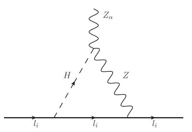
For the weak magnetic dipole moment, we also use diagrams like those shown in FIG.[1] with the photon replaced by the Z boson, but we must also consider the diagrams shown in FIG.[2]
Refer to caption
(d)
Refer to caption
(e)
Refer to caption
(f)
Figure 2: Additionally to the Feynman diagrams (a) y (b) there are contributions from (d), (e) y (f) to the weak dipole moment of the charged leptons aliWsubscriptsuperscript𝑎𝑊subscript𝑙𝑖a^{W}_{l_{i}}. In the Feynman diagrams (e) H=h0,H0,A0𝐻superscript0superscript𝐻0superscript𝐴0H=h^{0},\,H^{0},\,A^{0} and (f) H=h0,H0.𝐻superscript0superscript𝐻0H=h^{0},\,H^{0}.

The contributions to WMDM of the charged leptons of each Feynman diagram are given by:

(aliW)ρ1ρ2ρ3=a,b,c,eAa,b,c,e01𝑑x01x𝑑yGkρ1ρ2ρ3(x,y),superscriptsuperscriptsubscript𝑎subscript𝑙𝑖𝑊subscript𝜌1subscript𝜌2subscript𝜌3subscript𝑎𝑏𝑐𝑒subscript𝐴𝑎𝑏𝑐𝑒superscriptsubscript01differential-d𝑥superscriptsubscript01𝑥differential-d𝑦superscriptsubscript𝐺𝑘subscript𝜌1subscript𝜌2subscript𝜌3𝑥𝑦\left(a_{l_{i}}^{W}\right)^{\rho_{1}\rho_{2}\rho_{3}}=\sum_{a,\,b,\,c,\,e}A_{a,\,b,\,c,\,e}\intop_{0}^{1}dx\intop_{0}^{1-x}dy\,G_{k}^{\rho_{1}\rho_{2}\rho_{3}}(x,\,y), (81)

again the label ρnsubscript𝜌𝑛\rho_{n} refers to the particles circulating in a particular one-loop diagram, Aa,b,c,esubscript𝐴𝑎𝑏𝑐𝑒A_{a,\,b,\,\,c,\,e} represent terms associated to each Feynman diagram, given by

Aasubscript𝐴𝑎\displaystyle A_{a} =\displaystyle= mτ|ηllaρ1ρ2ρ3|24π2cWsW,subscript𝑚𝜏superscriptsuperscriptsubscript𝜂𝑙subscriptsuperscript𝑙𝑎subscript𝜌1subscript𝜌2subscript𝜌324superscript𝜋2subscript𝑐𝑊subscript𝑠𝑊\displaystyle\frac{m_{\tau}\left|\eta_{ll^{\prime}_{a}}^{\rho_{1}\rho_{2}\rho_{3}}\right|^{2}}{4\pi^{2}c_{W}s_{W}}, (82)
Absubscript𝐴𝑏\displaystyle A_{b} =\displaystyle= mτ3gW3(cW2sW2)32π2mW2cW,superscriptsubscript𝑚𝜏3superscriptsubscript𝑔𝑊3superscriptsubscript𝑐𝑊2superscriptsubscript𝑠𝑊232superscript𝜋2superscriptsubscript𝑚𝑊2subscript𝑐𝑊\displaystyle\frac{m_{\tau}^{3}g_{W}^{3}(c_{W}^{2}-s_{W}^{2})}{32\pi^{2}m_{W}^{2}c_{W}}, (83)
Adsubscript𝐴𝑑\displaystyle A_{d} =\displaystyle= gW2gZ128π2mW2cW,superscriptsubscript𝑔𝑊2subscript𝑔𝑍128superscript𝜋2superscriptsubscript𝑚𝑊2subscript𝑐𝑊\displaystyle\frac{g_{W}^{2}g_{Z}}{128\pi^{2}m_{W}^{2}c_{W}}, (84)
Afsubscript𝐴𝑓\displaystyle A_{f} =\displaystyle= mτemZηlmfρ1ρ2ρ34π2cW3sW2cos(αβ),subscript𝑚𝜏𝑒subscript𝑚𝑍superscriptsubscript𝜂𝑙subscript𝑚𝑓subscript𝜌1subscript𝜌2subscript𝜌34superscript𝜋2superscriptsubscript𝑐𝑊3superscriptsubscript𝑠𝑊2𝑐𝑜𝑠𝛼𝛽\displaystyle\frac{m_{\tau}em_{Z}\eta_{lm_{f}}^{\rho_{1}\rho_{2}\rho_{3}}}{4\pi^{2}c_{W}^{3}s_{W}^{2}}cos(\alpha-\beta), (85)

where cW,sW,mW,mZsubscript𝑐𝑊subscript𝑠𝑊subscript𝑚𝑊subscript𝑚𝑍c_{W},\,s_{W},\,m_{W},\,m_{Z} are the cosine, sine of the Weinberg angle, W and Z gauge boson mass, respectively. We omit Aesubscript𝐴𝑒A_{e} because the Feynman diagram (e) gives no contribution to weak magnetic dipole moment. The Gkρ1ρ2ρ3(x,y)superscriptsubscript𝐺𝑘subscript𝜌1subscript𝜌2subscript𝜌3𝑥𝑦G_{k}^{\rho_{1}\rho_{2}\rho_{3}}(x,\,y) functions are:

GaHljlj(x,y)superscriptsubscript𝐺𝑎𝐻subscript𝑙𝑗subscript𝑙𝑗𝑥𝑦\displaystyle G_{a}^{Hl_{j}l_{j}}(x,\,y) =\displaystyle= 2(CV(x+y)(mli(x+y1)mlj))/Ma2,2subscript𝐶𝑉𝑥𝑦subscript𝑚subscript𝑙𝑖𝑥𝑦1subscript𝑚subscript𝑙𝑗superscriptsubscript𝑀𝑎2\displaystyle-2(C_{V}(x+y)(m_{l_{i}}(x+y-1)-m_{l_{j}}))/M_{a}^{2}, (86)
GbH±H±ν(x,y)superscriptsubscript𝐺𝑏superscript𝐻plus-or-minussuperscript𝐻plus-or-minus𝜈𝑥𝑦\displaystyle G_{b}^{H^{\pm}H^{\pm}\nu}(x,\,y) =\displaystyle= 4mlix(x1)/Mb2,4subscript𝑚subscript𝑙𝑖𝑥𝑥1superscriptsubscript𝑀𝑏2\displaystyle 4m_{l_{i}}x(x-1)/M_{b}^{2}, (87)
GdH±νν(x,y)superscriptsubscript𝐺𝑑superscript𝐻plus-or-minus𝜈𝜈𝑥𝑦\displaystyle G_{d}^{H^{\pm}\nu\nu}(x,\,y) =\displaystyle= 8mli(x+y1)(x+y)/Md2,8subscript𝑚subscript𝑙𝑖𝑥𝑦1𝑥𝑦superscriptsubscript𝑀𝑑2\displaystyle-8m_{l_{i}}(x+y-1)(x+y)/M_{d}^{2}, (88)
GfZHτ(x,y)superscriptsubscript𝐺𝑓𝑍𝐻𝜏𝑥𝑦\displaystyle G_{f}^{ZH\tau}(x,\,y) =\displaystyle= CVmZ2Mf2(mli2((x+y1)2(x+y1)\displaystyle-\frac{C_{V}}{m_{Z}^{2}M_{f}^{2}}(-m_{l_{i}}^{2}((x+y-1)^{2}(x+y-1)
+\displaystyle+ Mf2(log(Mf2)(23(x+y))xy1)+mZ2x(y(x+y1)+2)),\displaystyle M_{f}^{2}(\log(M_{f}^{2})(2-3(x+y))-x-y-1)+m_{Z}^{2}x(y(x+y-1)+2)),

where

Ma2superscriptsubscript𝑀𝑎2\displaystyle M_{a}^{2} =\displaystyle= mli2(x+y1)(x+y)+mlj(x+y)mZ2xymH2(x+y1),superscriptsubscript𝑚subscript𝑙𝑖2𝑥𝑦1𝑥𝑦subscript𝑚subscript𝑙𝑗𝑥𝑦superscriptsubscript𝑚𝑍2𝑥𝑦superscriptsubscript𝑚𝐻2𝑥𝑦1\displaystyle m_{l_{i}}^{2}(x+y-1)(x+y)+m_{l_{j}}(x+y)-m_{Z}^{2}xy-m_{H}^{2}(x+y-1), (90)
Mb2superscriptsubscript𝑀𝑏2\displaystyle M_{b}^{2} =\displaystyle= mli2(x1)x+mZ2y(x+y1)mH2(x1),superscriptsubscript𝑚subscript𝑙𝑖2𝑥1𝑥superscriptsubscript𝑚𝑍2𝑦𝑥𝑦1superscriptsubscript𝑚𝐻2𝑥1\displaystyle m_{l_{i}}^{2}(x-1)x+m_{Z}^{2}y(x+y-1)-m_{H}^{2}(x-1), (91)
Md2superscriptsubscript𝑀𝑑2\displaystyle M_{d}^{2} =\displaystyle= mli2(x+y1)(x+y)mZ2xymH2(x+y1),superscriptsubscript𝑚subscript𝑙𝑖2𝑥𝑦1𝑥𝑦superscriptsubscript𝑚𝑍2𝑥𝑦superscriptsubscript𝑚𝐻2𝑥𝑦1\displaystyle m_{l_{i}}^{2}(x+y-1)(x+y)-m_{Z}^{2}xy-m_{H}^{2}(x+y-1), (92)
Mf2superscriptsubscript𝑀𝑓2\displaystyle M_{f}^{2} =\displaystyle= mli2((x+y1)(x+y1))mZ2x(y1)+mH2y.superscriptsubscript𝑚subscript𝑙𝑖2𝑥𝑦1𝑥𝑦1superscriptsubscript𝑚𝑍2𝑥𝑦1superscriptsubscript𝑚𝐻2𝑦\displaystyle m_{l_{i}}^{2}((x+y-1)(x+y-1))-m_{Z}^{2}x(y-1)+m_{H}^{2}y. (93)

The total contribution to (aτW)superscriptsubscript𝑎𝜏𝑊(a_{\tau}^{W}) is:

(aτW)THDMIII=(aτW)H±H±ν+H=h0,H0,A0lj=e,μ,τ(aτW)Hljlj+(aτW)H±νν+(aτW)ZHτ.superscriptsuperscriptsubscript𝑎𝜏𝑊𝑇𝐻𝐷𝑀𝐼𝐼𝐼superscriptsuperscriptsubscript𝑎𝜏𝑊superscript𝐻plus-or-minussuperscript𝐻plus-or-minus𝜈subscript𝑙𝑗𝑒𝜇𝜏𝐻superscript0superscript𝐻0superscript𝐴0superscriptsuperscriptsubscript𝑎𝜏𝑊𝐻subscript𝑙𝑗subscript𝑙𝑗superscriptsuperscriptsubscript𝑎𝜏𝑊superscript𝐻plus-or-minus𝜈𝜈superscriptsuperscriptsubscript𝑎𝜏𝑊𝑍𝐻𝜏(a_{\tau}^{W})^{THDM-III}=(a_{\tau}^{W})^{H^{\pm}H^{\pm}\nu}+\underset{\underset{l_{j}=e,\,\mu,\,\tau}{H=h^{0},\,H^{0},\,A^{0}}}{\sum}(a_{\tau}^{W})^{Hl_{j}l_{j}}+(a_{\tau}^{W})^{H^{\pm}\nu\nu}+(a_{\tau}^{W})^{ZH\tau}. (94)

IV Constraints from Low Energy Processes

Due to the introduction of a second scalar doublet, there are additional Feynman diagrams that are not present in the SM, involving the exchange of Higgs bosons (h0,H0,A0,H±superscript0superscript𝐻0superscript𝐴0superscript𝐻plus-or-minush^{0},\,H^{0},\,A^{0},\,H^{\pm}). There are currently strict bounds and measurements that have been obtained through various low energy phenomenological studies, this allows us to constraint parameters of the model such as tanβ(=tβ)=v2/v1annotated𝛽absentsubscript𝑡𝛽subscript𝑣2subscript𝑣1\tan{\beta}(=t_{\beta})=v_{2}/v_{1} which controls the intensity of the coupling of the Higgs bosons to the fermions. In this section we show the allowed parameters space in the plane tβmH(H±)subscript𝑡𝛽subscript𝑚𝐻superscript𝐻plus-or-minust_{\beta}-m_{H(H^{\pm})}, the other parameters are fixed. In particular for α𝛼\alpha and β𝛽\beta angles we study the scenario where αβ=π2𝛼𝛽𝜋2\alpha-\beta=\frac{\pi}{2}, which reproduces the case where the coupling of h0superscript0h^{0} to fermions is SM-like. In general, the favored region for THDM’s are phenomenologically viable for the scenario αβ=π2𝛼𝛽𝜋2\alpha-\beta=\frac{\pi}{2} [27]. We consider the relevant low energy constraints and the muon anomalous magnetic dipole moment for constraint the model parameters and then we give analytical predictions to magnetic and weak magnetic dipole moments of charged leptons in the section[V] using values of the allowed region. For the low energy constraints mediated by neutral Higgs bosons, we consider Bs0μμ¯superscriptsubscript𝐵𝑠0𝜇¯𝜇B_{s}^{0}\to\mu\bar{\mu}, μeγ𝜇𝑒𝛾\mu\rightarrow e\gamma, τμγ𝜏𝜇𝛾\tau\rightarrow\mu\gamma, τeγ𝜏𝑒𝛾\tau\rightarrow e\gamma, KK¯𝐾¯𝐾K-\bar{K} mixing and liljlklk¯subscript𝑙𝑖subscript𝑙𝑗subscript𝑙𝑘¯subscript𝑙𝑘l_{i}\rightarrow l_{j}l_{k}\overline{l_{k}} and the rare Higgs decay hτμ𝜏𝜇h\to\tau\mu. While for processes mediated by charged Higgs bosons bsγ𝑏𝑠𝛾b\to s\gamma and BD(D)τν𝐵𝐷superscript𝐷𝜏𝜈B\to D(D^{*})\tau\nu. The processes H02jets,Zff¯,e+eH0Z,H0A0,e+ebb¯Hformulae-sequencesuperscript𝐻02𝑗𝑒𝑡𝑠formulae-sequence𝑍𝑓¯𝑓formulae-sequencesuperscript𝑒superscript𝑒superscript𝐻0𝑍superscript𝐻0superscript𝐴0superscript𝑒superscript𝑒𝑏¯𝑏𝐻H^{0}\to 2\,jets,\,Z\to f\bar{f},\,e^{+}e^{-}\to H^{0}Z,\,H^{0}A^{0},\,e^{+}e^{-}\to b\bar{b}H impose a limit on the mass of the Higgs boson given by mH0>110.6GeVsubscript𝑚superscript𝐻0110.6𝐺𝑒𝑉m_{H^{0}}>110.6\,GeV at 95% [28] and in the range 155GeV155𝐺𝑒𝑉1-55\,GeV is excluded [29].

On the other hand, a theoretical approach that can be used to try and understand the underlying physics is through the effective Hamiltonian,

eff=GF2iVCKMiCi(μ)Qi,subscript𝑒𝑓𝑓subscript𝐺𝐹2subscript𝑖superscriptsubscript𝑉𝐶𝐾𝑀𝑖subscript𝐶𝑖𝜇subscript𝑄𝑖\mathcal{H}_{eff}=\frac{G_{F}}{\sqrt{2}}\sum_{i}V_{CKM}^{i}C_{i}(\mu)Q_{i}, (95)

where Qisubscript𝑄𝑖Q_{i} are the operators which govern the decay and Ci(μ)subscript𝐶𝑖𝜇C_{i}(\mu) are Wilson Coefficients. The scale μ𝜇\mu separates the physics contributions into short distance contributions contained in Ci(μ)subscript𝐶𝑖𝜇C_{i}(\mu) while the long distance contributions are contained in Qisubscript𝑄𝑖Q_{i} but the Wilson Coefficients depend on the couplings of the particular model, which in our case are functions of α𝛼\alpha, β𝛽\beta, θisubscript𝜃𝑖\theta_{i}, mH(H±)subscript𝑚𝐻superscript𝐻plus-or-minusm_{H(H^{\pm})} and γfsubscript𝛾𝑓\gamma_{f}. This will allow us to constrain the model parameters.

IV.1 Low energy constraints mediated by neutral Higgs bosons

IV.1.1 Bs0μμ¯superscriptsubscript𝐵𝑠0𝜇¯𝜇B_{s}^{0}\to\mu\bar{\mu}

A measurement of Bs0μμ¯superscriptsubscript𝐵𝑠0𝜇¯𝜇B_{s}^{0}\rightarrow\mu\overline{\mu} was reported in [35], whose value is

BR(Bs0μμ¯)=(2.80.6+0.7)×109,𝐵𝑅superscriptsubscript𝐵𝑠0𝜇¯𝜇superscriptsubscript2.80.60.7superscript109BR(B_{s}^{0}\rightarrow\mu\bar{\mu})=(2{.}8_{-0{.}6}^{+0{.}7})\times 10^{-9}, (96)

while the SM value is given by [36]

BR(Bs0μμ¯)SM=(3.23±0.27)×109,𝐵𝑅subscriptsuperscriptsubscript𝐵𝑠0𝜇¯𝜇𝑆𝑀plus-or-minus3.230.27superscript109BR(B_{s}^{0}\rightarrow\mu\bar{\mu})_{SM}=(3{.}23\pm 0{.}27)\times 10^{-9}, (97)

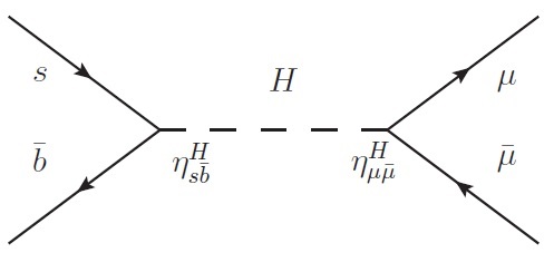
which puts very stringent constraints on the model. The Feynman diagram for this process at the quark level is shown in FIG.[3].
Refer to caption
Figure 3: Feynman diagram for the Bs0μμ¯superscriptsubscript𝐵𝑠0𝜇¯𝜇B_{s}^{0}\to\mu\bar{\mu} process at the quark level. The labels ηff¯Hsuperscriptsubscript𝜂𝑓¯𝑓𝐻\eta_{f\bar{f}}^{H} indicate the new contributions coming from the THDM-III. We will omit these labels in all further Feynman diagrams.

We observe that the new contributions from Higgs bosons appear in the Hs¯b𝐻¯𝑠𝑏H\bar{s}b and Hμμ¯𝐻𝜇¯𝜇H\mu\bar{\mu} couplings. The Branching ratio for this decay is given by [37],

BR𝐵𝑅\displaystyle BR (Bs0μ¯μ)=GF2αem216π3MBτB|VtbVts|214mμ2MB2superscriptsubscript𝐵𝑠0¯𝜇𝜇superscriptsubscript𝐺𝐹2superscriptsubscript𝛼𝑒𝑚216superscript𝜋3subscript𝑀𝐵subscript𝜏𝐵superscriptsubscript𝑉𝑡𝑏superscriptsubscript𝑉𝑡𝑠214superscriptsubscript𝑚𝜇2superscriptsubscript𝑀𝐵2\displaystyle\left(B_{s}^{0}\rightarrow\bar{\mu}\mu\right)=\frac{G_{F}^{2}\alpha_{em}^{2}}{16\pi^{3}}M_{B}\tau_{B}\left|V_{tb}V_{ts}^{*}\right|^{2}\sqrt{1-\frac{4m_{\mu}^{2}}{M_{B}^{2}}} (98)
×\displaystyle\times [|FH|2(14mμ2MB2)+|FA0|2],delimited-[]superscriptsubscript𝐹𝐻214superscriptsubscript𝑚𝜇2superscriptsubscript𝑀𝐵2superscriptsubscript𝐹superscript𝐴02\displaystyle\left[\left|F_{H}\right|^{2}\left(1-\frac{4m_{\mu}^{2}}{M_{B}^{2}}\right)+\left|F_{A^{0}}\right|^{2}\right],

where FHsubscript𝐹𝐻F_{H} and FA0subscript𝐹superscript𝐴0F_{A^{0}} are the form factors given by,

FH,A0subscript𝐹𝐻superscript𝐴0\displaystyle F_{H,A^{0}} =\displaystyle= i2MB2fBsmbmb+msCH,A0,𝑖2superscriptsubscript𝑀𝐵2subscript𝑓subscript𝐵𝑠subscript𝑚𝑏subscript𝑚𝑏subscript𝑚𝑠subscript𝐶𝐻superscript𝐴0\displaystyle-\frac{i}{2}M_{B}^{2}\,f_{B_{s}}\frac{m_{b}}{m_{b}+m_{s}}C_{H,A^{0}},

where GFsubscript𝐺𝐹G_{F} is the Fermi constant, τBsubscript𝜏𝐵\tau_{B} the lifetime of the B𝐵B meson, MBsubscript𝑀𝐵M_{B} the B meson mass, fBs=0.256subscript𝑓subscript𝐵𝑠0.256f_{B_{s}}=0{.}256 and CH,CA0subscript𝐶𝐻subscript𝐶superscript𝐴0C_{H},\;\;C_{A^{0}} the Wilson coefficients that appear in the effective Hamiltonian,

Heff=22GFVtbVtsiCiQi,subscript𝐻𝑒𝑓𝑓22subscript𝐺𝐹subscript𝑉𝑡𝑏superscriptsubscript𝑉𝑡𝑠subscript𝑖subscript𝐶𝑖subscript𝑄𝑖H_{eff}=-2\sqrt{2}G_{F}V_{tb}V_{ts}^{*}\sum_{i}C_{i}Q_{i}, (100)

where Qisubscript𝑄𝑖Q_{i} are the effective operators and are given by:

QH=e216π2mb(s¯PRb)(μ¯μ),QA0=e216π2mb(s¯PRb)(μ¯γ5μ)formulae-sequencesubscript𝑄𝐻superscript𝑒216superscript𝜋2subscript𝑚𝑏¯𝑠subscript𝑃𝑅𝑏¯𝜇𝜇subscript𝑄superscript𝐴0superscript𝑒216superscript𝜋2subscript𝑚𝑏¯𝑠subscript𝑃𝑅𝑏¯𝜇superscript𝛾5𝜇Q_{H}=\frac{e^{2}}{16\pi^{2}}m_{b}(\bar{s\,}P_{R}b)(\bar{\mu}\,\mu),\;Q_{A^{0}}=\frac{e^{2}}{16\pi^{2}}m_{b}(\bar{s\,}P_{R}b)(\bar{\mu}\gamma^{5}\mu)

and the Wilson coefficients Cisubscript𝐶𝑖C_{i} are,

CH=2πmμVtsVtbαem[14mH02H=H0,h0ηb¯sHηmm¯H],CA0=2πmμVtsVtbαem[14mA02ηb¯sA0ηmm¯A0],formulae-sequencesubscript𝐶𝐻2𝜋subscript𝑚𝜇superscriptsubscript𝑉𝑡𝑠subscript𝑉𝑡𝑏subscript𝛼𝑒𝑚delimited-[]14superscriptsubscript𝑚superscript𝐻02subscript𝐻superscript𝐻0superscript0superscriptsubscript𝜂¯𝑏𝑠𝐻superscriptsubscript𝜂𝑚¯𝑚𝐻subscript𝐶superscript𝐴02𝜋subscript𝑚𝜇superscriptsubscript𝑉𝑡𝑠subscript𝑉𝑡𝑏subscript𝛼𝑒𝑚delimited-[]14superscriptsubscript𝑚superscript𝐴02superscriptsubscript𝜂¯𝑏𝑠superscript𝐴0superscriptsubscript𝜂𝑚¯𝑚superscript𝐴0C_{H}=\frac{2\pi m_{\mu}}{V_{ts}^{*}V_{tb}\alpha_{em}}\Bigg{[}\frac{1}{4m_{H^{0}}^{2}}\sum_{H=H^{0},\,h^{0}}\eta_{\bar{b}s}^{H}\eta_{m\bar{m}}^{H}\Bigg{]},\;C_{A^{0}}=\frac{2\pi m_{\mu}}{V_{ts}^{*}V_{tb}\alpha_{em}}\Bigg{[}\frac{1}{4m_{A^{0}}^{2}}\eta_{\bar{b}s}^{A^{0}}\eta_{m\bar{m}}^{A^{0}}\Bigg{]}, (101)

where mb,Vtb(ts),mH0,mh0,mA0subscript𝑚𝑏subscriptsuperscript𝑉𝑡𝑏𝑡𝑠subscript𝑚superscript𝐻0subscript𝑚superscript0subscript𝑚superscript𝐴0m_{b},\,V^{*}_{tb(ts)},m_{H^{0}},m_{h^{0}},m_{A^{0}} are bottom quark mass, CKM elements, heavy, SM-like, pseudo scalar Higgs bosons mass, respectively. We can see through 101 the dependence on the model parameters since ηff¯H,A0=ηff¯H,A0(α,β,θi,γf)superscriptsubscript𝜂𝑓¯𝑓𝐻superscript𝐴0superscriptsubscript𝜂𝑓¯𝑓𝐻superscript𝐴0𝛼𝛽subscript𝜃𝑖subscript𝛾𝑓\eta_{f\bar{f}}^{H,A^{0}}=\eta_{f\bar{f}}^{H,A^{0}}(\alpha,\,\beta,\,\theta_{i},\,\gamma_{f}) and therefore CH,A0=CH,A0(α,β,θi,mH,γf)subscript𝐶𝐻superscript𝐴0subscript𝐶𝐻superscript𝐴0𝛼𝛽subscript𝜃𝑖subscript𝑚𝐻subscript𝛾𝑓C_{H,A^{0}}=C_{H,A^{0}}(\alpha,\,\beta,\,\theta_{i},\,m_{H},\gamma_{f}).

IV.1.2 Radiative decays liljγsubscript𝑙𝑖subscript𝑙𝑗𝛾l_{i}\to l_{j}\gamma

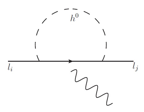
The second processes that we considered are the radiative decays liljγsubscript𝑙𝑖subscript𝑙𝑗𝛾l_{i}\to l_{j}\gamma. The Feynman diagram with the largest contributions for this process is shown in FIG.[4],
Refer to caption
Figure 4: Feynman diagram for the liljγsubscript𝑙𝑖subscript𝑙𝑗𝛾l_{i}\to l_{j}\gamma process.

The branching ratio for the general decay of a lepton (lisubscript𝑙𝑖l_{i}) to a lepton of a different family (ljsubscript𝑙𝑗l_{j}) is given by: [38]

Br(liljγ)=mli54πΓli(|CRljli|2+|CLljli|2),𝐵𝑟subscript𝑙𝑖subscript𝑙𝑗𝛾superscriptsubscript𝑚subscript𝑙𝑖54𝜋subscriptΓsubscript𝑙𝑖superscriptsuperscriptsubscript𝐶𝑅subscript𝑙𝑗subscript𝑙𝑖2superscriptsuperscriptsubscript𝐶𝐿subscript𝑙𝑗subscript𝑙𝑖2\displaystyle Br(l_{i}\to l_{j}\gamma)=\frac{m_{l_{i}}^{5}}{4\pi\Gamma_{l_{i}}}\left(\big{|}C_{R}^{l_{j}l_{i}}\big{|}^{2}+\big{|}C_{L}^{l_{j}l_{i}}\big{|}^{2}\right), (102)

where the Wilson Coefficients CR,Lljlisuperscriptsubscript𝐶𝑅𝐿subscript𝑙𝑗subscript𝑙𝑖C_{R,L}^{l_{j}l_{i}} are:

CRHljlisuperscriptsubscript𝐶𝑅𝐻subscript𝑙𝑗subscript𝑙𝑖\displaystyle C_{RH}^{l_{j}l_{i}} =\displaystyle= [ηliljLRHηliljLRH+ηljliLRHηljliLRH\displaystyle\Bigg{[}\eta_{l_{i}l_{j}}^{LRH\star}\eta_{l_{i}l_{j}}^{LRH}+\eta_{l_{j}l_{i}}^{LRH\star}\eta_{l_{j}l_{i}}^{LRH} (103)
\displaystyle- mlimliηliljLRHηljliLRH(9+6ln(mlj2mH2))],\displaystyle\frac{m_{l_{i}}}{m_{l_{i}}}\eta_{l_{i}l_{j}}^{LRH}\eta_{l_{j}l_{i}}^{LRH}\left(9+6\ln\left(\frac{m_{l_{j}}^{2}}{m_{H}^{2}}\right)\right)\Bigg{]},

such that H=h0,H0,A0𝐻superscript0superscript𝐻0superscript𝐴0H=h^{0},H^{0},A^{0}. CLljlisuperscriptsubscript𝐶𝐿subscript𝑙𝑗subscript𝑙𝑖C_{L}^{l_{j}l_{i}} is obtained by simply interchanging R by L.

The experimental bounds for each of the different processes are [39], [40], [41]

BR(τμγ)𝐵𝑅𝜏𝜇𝛾\displaystyle BR(\tau\rightarrow\mu\gamma) \displaystyle\leq 4.5×1084.5superscript108\displaystyle 4{.}5\times 10^{-8}
BR(τeγ)𝐵𝑅𝜏𝑒𝛾\displaystyle BR(\tau\rightarrow e\gamma) \displaystyle\leq 1.1×1071.1superscript107\displaystyle 1{.}1\times 10^{-7}
BR(μeγ)𝐵𝑅𝜇𝑒𝛾\displaystyle BR(\mu\rightarrow e\gamma) \displaystyle\leq 5.7×10135.7superscript1013\displaystyle 5{.}7\times 10^{-13}

Again we can see that CRHljli=CRHljli(α,β,θi,mH,γf)superscriptsubscript𝐶𝑅𝐻subscript𝑙𝑗subscript𝑙𝑖superscriptsubscript𝐶𝑅𝐻subscript𝑙𝑗subscript𝑙𝑖𝛼𝛽subscript𝜃𝑖subscript𝑚𝐻subscript𝛾𝑓C_{RH}^{l_{j}l_{i}}=C_{RH}^{l_{j}l_{i}}(\alpha,\,\beta,\,\theta_{i},\,m_{H},\gamma_{f}).

IV.1.3 KK¯𝐾¯𝐾K-\bar{K} mixing

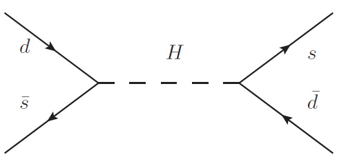
The amplitude for KK¯𝐾¯𝐾K\bar{K} Mixing receives contributions from the Feynman diagram shown in FIG.[5].
Refer to caption
Figure 5: Feynman diagram for the KK¯mixing𝐾¯𝐾𝑚𝑖𝑥𝑖𝑛𝑔K\bar{K}-mixing.

The effective hamiltonian for this process at the quark level is written from [42] as follows

HeffΔS=2=GF2MW216π2iCiQi,superscriptsubscript𝐻𝑒𝑓𝑓Δ𝑆2superscriptsubscript𝐺𝐹2superscriptsubscript𝑀𝑊216superscript𝜋2subscript𝑖subscript𝐶𝑖subscript𝑄𝑖\displaystyle H_{eff}^{\Delta S=2}=\frac{G_{F}^{2}M_{W}^{2}}{16\pi^{2}}\sum_{i}C_{i}Q_{i}, (104)

with (i=L,R,LR)𝑖𝐿𝑅𝐿𝑅(i=L,R,LR), where

QLs¯d,sd¯superscriptsubscript𝑄𝐿¯𝑠𝑑𝑠¯𝑑\displaystyle Q_{L}^{\overline{s}d,s\overline{d}} =\displaystyle= (s¯PLd)(s¯PLd),¯𝑠subscript𝑃𝐿𝑑¯𝑠subscript𝑃𝐿𝑑\displaystyle\big{(}\bar{s}P_{L}d\big{)}\big{(}\bar{s}P_{L}d\big{)}, (105)
QRs¯d,sd¯superscriptsubscript𝑄𝑅¯𝑠𝑑𝑠¯𝑑\displaystyle Q_{R}^{\overline{s}d,s\overline{d}} =\displaystyle= (s¯PRd)(s¯PRd),¯𝑠subscript𝑃𝑅𝑑¯𝑠subscript𝑃𝑅𝑑\displaystyle\big{(}\bar{s}P_{R}d\big{)}\big{(}\bar{s}P_{R}d\big{)}, (106)
QLRs¯d,sd¯superscriptsubscript𝑄𝐿𝑅¯𝑠𝑑𝑠¯𝑑\displaystyle Q_{LR}^{\overline{s}d,s\overline{d}} =\displaystyle= (s¯PLd)(s¯PRd),¯𝑠subscript𝑃𝐿𝑑¯𝑠subscript𝑃𝑅𝑑\displaystyle\big{(}\bar{s}P_{L}d\big{)}\big{(}\bar{s}P_{R}d\big{)}, (107)

and the Wilson coefficients are written here for a general multi-Higgs doublet model,

CLs¯d,sd¯=16π2GF2mW2msmd|ηsbH|2a=12(U1a)2mH2,superscriptsubscript𝐶𝐿¯𝑠𝑑𝑠¯𝑑16superscript𝜋2superscriptsubscript𝐺𝐹2superscriptsubscript𝑚𝑊2subscript𝑚𝑠subscript𝑚𝑑superscriptsuperscriptsubscript𝜂𝑠𝑏𝐻2superscriptsubscript𝑎12superscriptsuperscriptsubscript𝑈1𝑎2superscriptsubscript𝑚𝐻2\displaystyle C_{L}^{\overline{s}d,s\overline{d}}=-\frac{16\pi^{2}}{G_{F}^{2}m_{W}^{2}}m_{s}m_{d}|\eta_{sb}^{H}|^{2}\sum_{a=1}^{2}\frac{\big{(}U_{1a}^{*}\big{)}^{2}}{m_{H}^{2}}, (108)
CRs¯d,sd¯=16π2GF2mW2msmd|ηsbH|2a=12(U1a)2mH2,superscriptsubscript𝐶𝑅¯𝑠𝑑𝑠¯𝑑16superscript𝜋2superscriptsubscript𝐺𝐹2superscriptsubscript𝑚𝑊2subscript𝑚𝑠subscript𝑚𝑑superscriptsuperscriptsubscript𝜂𝑠𝑏𝐻2superscriptsubscript𝑎12superscriptsubscript𝑈1𝑎2superscriptsubscript𝑚𝐻2\displaystyle C_{R}^{\overline{s}d,s\overline{d}}=-\frac{16\pi^{2}}{G_{F}^{2}m_{W}^{2}}m_{s}m_{d}|\eta_{sb}^{H}|^{2}\sum_{a=1}^{2}\frac{\big{(}U_{1a}\big{)}^{2}}{m_{H}^{2}}, (109)
CLRs¯d,sd¯=16π2GF2mW2msmd|ηsbH|2a=12U1aU1amH2,superscriptsubscript𝐶𝐿𝑅¯𝑠𝑑𝑠¯𝑑16superscript𝜋2superscriptsubscript𝐺𝐹2superscriptsubscript𝑚𝑊2subscript𝑚𝑠subscript𝑚𝑑superscriptsuperscriptsubscript𝜂𝑠𝑏𝐻2superscriptsubscript𝑎12superscriptsubscript𝑈1𝑎subscript𝑈1𝑎superscriptsubscript𝑚𝐻2\displaystyle C_{LR}^{\overline{s}d,s\overline{d}}=-\frac{16\pi^{2}}{G_{F}^{2}m_{W}^{2}}m_{s}m_{d}|\eta_{sb}^{H}|^{2}\sum_{a=1}^{2}\frac{U_{1a}^{*}U_{1a}}{m_{H}^{2}}, (110)

where H=H0,h0,A0𝐻superscript𝐻0superscript0superscript𝐴0H=H^{0},\,h^{0},\,A^{0}. Ubasubscript𝑈𝑏𝑎U_{ba} is the rotation matrix to go from weak to mass-eigenstates in the neutral CP-even Higgs sector, since we are working in general THDM, the rotation matrix for neutral Higgs bosons takes the form

U=(cosαsinαsinαcosα).𝑈matrix𝛼𝛼𝛼𝛼\displaystyle U=\begin{pmatrix}\cos\alpha&-\sin\alpha\\ \sin\alpha&\cos\alpha\\ \end{pmatrix}.

Flavor violation arises from the non-diagonal terms of the K (neutral kaon) mass matrix, in particular the component M12K,superscriptsubscript𝑀12𝐾M_{12}^{K}, whose experimental value has been measured to be

M12K=ΔMKMK=7.2948×10¹⁵GeV,superscriptsubscript𝑀12𝐾Δsubscript𝑀𝐾subscript𝑀𝐾7.2948superscript1015𝐺𝑒𝑉\displaystyle M_{12}^{K}=\frac{\Delta M_{K}}{M_{K}}=7{.}2948\times 10^{-15}GeV, (111)

but given that ΔMKΔsubscript𝑀𝐾\Delta M_{K} is obtained through

ΔMKΔsubscript𝑀𝐾\displaystyle\Delta M_{K} =\displaystyle= 2ReK¯0|HeffΔS=2|K02𝑅𝑒quantum-operator-productsuperscript¯𝐾0superscriptsubscript𝐻𝑒𝑓𝑓Δ𝑆2superscript𝐾0\displaystyle 2Re\langle\bar{K}^{0}|H_{eff}^{\Delta S=2}|K^{0}\rangle (112)
=\displaystyle= GF2MW212π2MKFK2η2BKsuperscriptsubscript𝐺𝐹2superscriptsubscript𝑀𝑊212superscript𝜋2subscript𝑀𝐾superscriptsubscript𝐹𝐾2subscript𝜂2subscript𝐵𝐾\displaystyle\frac{G_{F}^{2}M_{W}^{2}}{12\pi^{2}}M_{K}F_{K}^{2}\eta_{2}{B}_{K}
×\displaystyle\times [P¯2,LRCLRs¯d,sd¯+P¯1,L(CLs¯d,sd¯+CRs¯d,sd¯)],delimited-[]subscript¯𝑃2𝐿𝑅superscriptsubscript𝐶𝐿𝑅¯𝑠𝑑𝑠¯𝑑subscript¯𝑃1𝐿superscriptsubscript𝐶𝐿¯𝑠𝑑𝑠¯𝑑superscriptsubscript𝐶𝑅¯𝑠𝑑𝑠¯𝑑\displaystyle\left[\bar{P}_{2,LR}C_{LR}^{\overline{s}d,s\overline{d}}+\bar{P}_{1,L}\left(C_{L}^{\overline{s}d,s\overline{d}}+C_{R}^{\overline{s}d,s\overline{d}}\right)\right],

where FK=160subscript𝐹𝐾160F_{K}=160 MeV, MK=497.6subscript𝑀𝐾497.6M_{K}=497{.}6 MeV, η2=0.57,BK=0.85±0.15,P¯2,LR=30.6formulae-sequencesubscript𝜂20.57formulae-sequencesubscript𝐵𝐾plus-or-minus0.850.15subscript¯𝑃2𝐿𝑅30.6\eta_{2}=0{.}57,\;\;{B}_{K}=0{.}85\pm 0{.}15,\;\;\bar{P}_{2,LR}=30{.}6 and P¯1,L=9.3.subscript¯𝑃1𝐿9.3\bar{P}_{1,L}=-9{.}3{.}, we have

M12Ksuperscriptsubscript𝑀12𝐾\displaystyle M_{12}^{K} =\displaystyle= 43FK2η2B¯K(mdms)1(vcosβ)243subscriptsuperscript𝐹2𝐾subscript𝜂2subscript¯𝐵𝐾subscript𝑚𝑑subscript𝑚𝑠1superscript𝑣𝑐𝑜𝑠𝛽2\displaystyle\frac{4}{3}F^{2}_{K}\eta_{2}\bar{B}_{K}\big{(}m_{d}m_{s}\big{)}\frac{1}{(vcos\beta)^{2}} (113)
×\displaystyle\times a=12[P¯2,LRU2aU1amH2+P¯1,L(U2a2mH2+U1a2mH2)].superscriptsubscript𝑎12delimited-[]subscript¯𝑃2𝐿𝑅subscript𝑈2𝑎subscript𝑈1𝑎superscriptsubscript𝑚𝐻2subscript¯𝑃1𝐿superscriptsubscript𝑈2𝑎2superscriptsubscript𝑚𝐻2superscriptsubscript𝑈1𝑎2superscriptsubscript𝑚𝐻2\displaystyle\sum_{a=1}^{2}\bigg{[}\bar{P}_{2,LR}\frac{U_{2a}U_{1a}}{m_{H}^{2}}+\bar{P}_{1,L}\bigg{(}\frac{U_{2a}^{2}}{m_{H}^{2}}+\frac{U_{1a}^{2}}{m_{H}^{2}}\bigg{)}\bigg{]}.

IV.1.4 liljlkl¯ksubscript𝑙𝑖subscript𝑙𝑗subscript𝑙𝑘subscript¯𝑙𝑘l_{i}\to l_{j}l_{k}\bar{l}_{k}

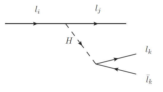
The Feynman diagram for the process liljlkl¯ksubscript𝑙𝑖subscript𝑙𝑗subscript𝑙𝑘subscript¯𝑙𝑘l_{i}\to l_{j}l_{k}\bar{l}_{k} is shown in the FIG.[6],

Refer to caption
Figure 6: Feynman diagram for the liljlkl¯ksubscript𝑙𝑖subscript𝑙𝑗subscript𝑙𝑘subscript¯𝑙𝑘l_{i}\to l_{j}l_{k}\bar{l}_{k} process.

The Branching ratio for this process including contributions from the three Higgs bosons is given by [43]

Br(li\displaystyle Br(l_{i} \displaystyle\rightarrow ljlkl¯k)=5δlllk+23τi211π3mljmlk2mli6v6{cos2(αβ)sin2αmh04\displaystyle l_{j}l_{k}\overline{l}_{k})=\frac{5\delta_{l_{l}l_{k}}+2}{3}\frac{\tau_{i}}{2^{11}\pi^{3}}\frac{m_{l_{j}}m_{l_{k}}^{2}m_{l_{i}}^{6}}{v^{6}}\left\{\frac{cos^{2}(\alpha-\beta)sin^{2}\alpha}{m_{h^{0}}^{4}}\right.
+\displaystyle+ sin2(αβ)cos2αmH042cos(αβ)sin(αβ)cosαsinαmh02mH02𝑠𝑖superscript𝑛2𝛼𝛽𝑐𝑜superscript𝑠2𝛼superscriptsubscript𝑚superscript𝐻042𝑐𝑜𝑠𝛼𝛽𝑠𝑖𝑛𝛼𝛽𝑐𝑜𝑠𝛼𝑠𝑖𝑛𝛼superscriptsubscript𝑚superscript02superscriptsubscript𝑚superscript𝐻02\displaystyle\frac{sin^{2}(\alpha-\beta)cos^{2}\alpha}{m_{H^{0}}^{4}}-2\frac{cos(\alpha-\beta)sin(\alpha-\beta)\,cos\alpha\,sin\alpha}{m_{h^{0}}^{2}m_{H^{0}}^{2}}
+\displaystyle+ sin2βmA04}|ηij|22cos4β.\displaystyle\left.\frac{sin^{2}\beta}{m_{A^{0}}^{4}}\right\}\frac{\left|\eta_{{ij}}\right|^{2}}{2cos^{4}\beta}.

where τisubscript𝜏𝑖\tau_{i} is the time life of the lisubscript𝑙𝑖l_{i} particle. The current upper bounds from PDG [44] are:

BR(τμμ¯μ)𝐵𝑅𝜏𝜇¯𝜇𝜇\displaystyle BR(\tau\rightarrow\mu\bar{\mu}\mu) <\displaystyle< 1.0×10121.0superscript1012\displaystyle 1{.}0\times 10^{-12}
BR(μee¯e)𝐵𝑅𝜇𝑒¯𝑒𝑒\displaystyle BR(\mu\rightarrow e\bar{e}e) <\displaystyle< 2.1×1082.1superscript108\displaystyle 2{.}1\times 10^{-8}

IV.2 Low energy constraints mediated by Charged Higgs bosons

IV.2.1 bsγ𝑏𝑠𝛾b\to s\gamma

In the Standard Model the dominant decay of b quarks are given via couplings to the Wsuperscript𝑊W^{-}. And rare decays like bsγ𝑏𝑠𝛾b\to s\gamma are described by penguin diagrams involving Wsuperscript𝑊W^{-} at one loop level, but in the THDM heavy charged Higgses also contribute at the one loop-level so the decay bsγ𝑏𝑠𝛾b\to s\gamma remains as a good candidate to probe BSM physics.

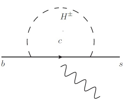
The Feynman diagram for bsγ𝑏𝑠𝛾b\to s\gamma involving Hsuperscript𝐻H^{-} is shown in FIG.[7].

Refer to caption
Figure 7: Feynman diagram for the bsγ𝑏𝑠𝛾b\to s\gamma.

The decay width is given by

Γ(bsγ)=GF232π4|VtsVtb|2αemmb5|D¯|2Γ𝑏𝑠𝛾superscriptsubscript𝐺𝐹232superscript𝜋4superscriptsuperscriptsubscript𝑉𝑡𝑠subscript𝑉𝑡𝑏2subscript𝛼𝑒𝑚superscriptsubscript𝑚𝑏5superscript¯𝐷2\displaystyle\Gamma(b\to s\gamma)=\frac{G_{F}^{2}}{32\pi^{4}}|V_{ts}^{\star}V_{tb}|^{2}\alpha_{em}m_{b}^{5}\big{|}\bar{D}\big{|}^{2} (114)

where the reduced amplitude D¯¯𝐷\bar{D} and the Wilson coefficients are presented in [45], and discussed in [46].

IV.2.2 BD(D)τν𝐵𝐷superscript𝐷𝜏𝜈B\rightarrow D(D^{*})\tau\nu

The BABAR𝐵𝐴𝐵𝐴𝑅BABAR collaboration [47] measured the branching ratios of the B𝐵B decays BR(BD(D)τν)𝐵𝑅𝐵𝐷superscript𝐷𝜏𝜈BR(B\to D(D^{*})\tau\nu), finding:

R(D)𝑅𝐷\displaystyle R(D) =\displaystyle= 0.44±0.058±0.042plus-or-minus0.440.0580.042\displaystyle 0{.}44\pm 0{.}058\pm 0{.}042 (115)
R(D)𝑅superscript𝐷\displaystyle R(D^{*}) =\displaystyle= 0.332±0.024±0.018.plus-or-minus0.3320.0240.018\displaystyle 0{.}332\pm 0{.}024\pm 0{.}018.

where

R(D(D))=BR(BD(D)τν)BR(BD(D)lν),𝑅𝐷superscript𝐷𝐵𝑅𝐵𝐷superscript𝐷𝜏𝜈𝐵𝑅𝐵𝐷superscript𝐷𝑙𝜈R(D(D^{*}))=\frac{BR(B\to D(D^{*})\tau\nu)}{BR(B\to D(D^{*})l\nu)}, (116)

with l=e,μ𝑙𝑒𝜇l=e,\,\mu, while the SM theoretical prediction for these processes is given by

RSM(D)subscript𝑅𝑆𝑀𝐷\displaystyle R_{SM}(D) =\displaystyle= 0.297±0.07,plus-or-minus0.2970.07\displaystyle 0{.}297\pm 0{.}07, (117)
RSM(D)subscript𝑅𝑆𝑀superscript𝐷\displaystyle R_{SM}(D^{*}) =\displaystyle= 0.252±0.003±0.018,plus-or-minus0.2520.0030.018\displaystyle 0{.}252\pm 0{.}003\pm 0{.}018,

taken together the results give a discrepancy of 3.4 σ𝜎\sigma. These processes are present in other models that involve charged scalar bosons and can be used to constrain the parameters of such models, like in our case of the THDM-III.

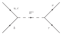
In this model the Feynman diagram that contributes to this process is shown in FIG.[8]
Refer to caption
Figure 8: Feynman diagram for the BD(D)τν𝐵𝐷superscript𝐷𝜏𝜈B\rightarrow D(D^{*})\tau\nu process.

These ratios can be expressed as follows,

R(D)𝑅𝐷\displaystyle{R}(D) =\displaystyle= RSM(D)subscript𝑅𝑆𝑀𝐷\displaystyle{R}_{SM}(D)
×\displaystyle\times (1+1.5Re[CRcb+CLcbCSMcb]+1.0|CRcb+CLcbCSMcb|2),11.5Redelimited-[]superscriptsubscript𝐶𝑅𝑐𝑏superscriptsubscript𝐶𝐿𝑐𝑏superscriptsubscript𝐶𝑆𝑀𝑐𝑏1.0superscriptsuperscriptsubscript𝐶𝑅𝑐𝑏superscriptsubscript𝐶𝐿𝑐𝑏superscriptsubscript𝐶𝑆𝑀𝑐𝑏2\displaystyle\left(1+1{.}5\;{\mbox{Re}}\left[\frac{C_{R}^{cb}+C_{L}^{cb}}{C_{SM}^{cb}}\right]+1{.}0\left|\frac{C_{R}^{cb}+C_{L}^{cb}}{C_{SM}^{cb}}\right|^{2}\right),
R(D)𝑅superscript𝐷\displaystyle{R}(D^{*}) =\displaystyle= RSM(D)subscript𝑅𝑆𝑀superscript𝐷\displaystyle{R}_{SM}(D^{*})
×\displaystyle\times (1+0.12Re[CRcbCLcbCSMcb]+0.05|CRcbCLcbCSMcb|2),10.12Redelimited-[]superscriptsubscript𝐶𝑅𝑐𝑏superscriptsubscript𝐶𝐿𝑐𝑏superscriptsubscript𝐶𝑆𝑀𝑐𝑏0.05superscriptsuperscriptsubscript𝐶𝑅𝑐𝑏superscriptsubscript𝐶𝐿𝑐𝑏superscriptsubscript𝐶𝑆𝑀𝑐𝑏2\displaystyle\left(1+0{.}12\;{\mbox{Re}}\left[\frac{C_{R}^{cb}-C_{L}^{cb}}{C_{SM}^{cb}}\right]+0{.}05\left|\frac{C_{R}^{cb}-C_{L}^{cb}}{C_{SM}^{cb}}\right|^{2}\right),

where CL,Rcbsuperscriptsubscript𝐶𝐿𝑅𝑐𝑏C_{L,R}^{cb} are the Wilson coefficients given in [48].

We find that this is the single most stringent low energy processes. Nonetheless, we are able to satisfy both R(D)𝑅𝐷R(D) and R(D)𝑅superscript𝐷R(D^{\star}) within our model. The combined allowed region of charged Higgs boson mass (mH±superscriptsubscript𝑚𝐻plus-or-minusm_{H}^{\pm}) and tβsubscript𝑡𝛽t_{\beta} for all the previous low energy processes are shown in the following section.

IV.3 h0τμsuperscript0𝜏𝜇h^{0}\to\tau\mu

The flavour violating decay h0τμsuperscript0𝜏𝜇h^{0}\to\tau\mu currently has an excess of signal events with a significance of 2.4 σ𝜎\sigma [49], whose branching ratio reported by CMS with a 95% confidence level is given by:

BR(h0τμ)<1.51%.𝐵𝑅superscript0𝜏𝜇percent1.51BR(h^{0}\to\tau\mu)<1.51\%. (120)

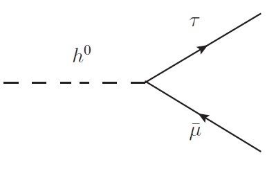
The tree level Feynman diagram for this process is shown in FIG.[9].
Refer to caption
(a)
Figure 9: Feynman diagram of h0τμsuperscript0𝜏𝜇h^{0}\to\tau\mu.

It is important to determine if our model acomodates this anomaly, to this purpuse we calculated the decay width given by:

Γ(h0τμ)Γsuperscript0𝜏𝜇\displaystyle\Gamma(h^{0}\to\tau\mu) =\displaystyle= Nc8πmh02|ητμh0|2(mh02(mτ+mμ)2)3/2subscript𝑁𝑐8𝜋superscriptsubscript𝑚superscript02superscriptsuperscriptsubscript𝜂𝜏𝜇superscript02superscriptsuperscriptsubscript𝑚superscript02superscriptsubscript𝑚𝜏subscript𝑚𝜇232\displaystyle\frac{N_{c}}{8\pi m_{h^{0}}^{2}}\Big{|}\eta_{\tau\mu}^{h^{0}}\Big{|}^{2}\left(m_{h^{0}}^{2}-(m_{\tau}+m_{\mu})^{2}\right)^{3/2} (121)
×\displaystyle\times (mh02(mτmμ)2)1/2,superscriptsuperscriptsubscript𝑚superscript02superscriptsubscript𝑚𝜏subscript𝑚𝜇212\displaystyle\left(m_{h^{0}}^{2}-(m_{\tau}-m_{\mu})^{2}\right)^{1/2},

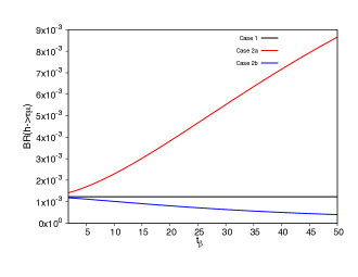
where Nc=1subscript𝑁𝑐1N_{c}=1 is the color number and mh0,mτ,mμsubscript𝑚superscript0subscript𝑚𝜏subscript𝑚𝜇m_{h^{0}},\,m_{\tau},\,m_{\mu} are the neutral light Higgs boson mass, tau mass and muon mass, respectively. We found that the Branching ratio for this process as a function of tβsubscript𝑡𝛽t_{\beta}, falls within the LHC reported measurement as shown in FIG.[10],
Refer to caption
(a)
Figure 10: Branching ratio of h0τμsuperscript0𝜏𝜇h^{0}\to\tau\mu decay as a function of tβsubscript𝑡𝛽t_{\beta}.

It might seem that the branching ratio for case 2a could grow in an undesirable way, but it becomes stable at the value of 2×10²²superscript1022\times 10^{-2}, while for the other two cases it decreases as tβsubscript𝑡𝛽t_{\beta} increases. The allowed range over tβsubscript𝑡𝛽t_{\beta} that we find in this process matches the allowed range obtained from the low energy process that will be presented in the following section.

IV.4 Allowed regions

  • tβsubscript𝑡𝛽t_{\beta} and mHsubscript𝑚𝐻m_{H}

We determine the allowed parameter space by first finding the allowed region for all of the low energy process: IV.1.1, IV.1.2, IV.1.3, IV.1.4 and we then intersect this region with the allowed space of aμTHDMIIIsuperscriptsubscript𝑎𝜇𝑇𝐻𝐷𝑀𝐼𝐼𝐼a_{\mu}^{THDM-III}. In the analysis we have worked with the γl=0.5,(αβ)=π2formulae-sequencesubscript𝛾𝑙0.5𝛼𝛽𝜋2\gamma_{l}=0.5,(\alpha-\beta)=\frac{\pi}{2} scenario, mH±=500GeVsubscript𝑚superscript𝐻plus-or-minus500𝐺𝑒𝑉m_{H^{\pm}}=500\,GeV ,mH=mH0,mA0,m_{H}=m_{H^{0}},m_{A^{0}}, θ1, 2=0subscript𝜃120\theta_{1,\,2}=0 and mh0=125GeVsubscript𝑚superscript0125𝐺𝑒𝑉m_{h^{0}}=125\,GeV; the selection of these values are reasonable, since they satisfy current experimental bounds [33] on both neutral and charged heavy Higgs.

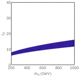
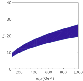
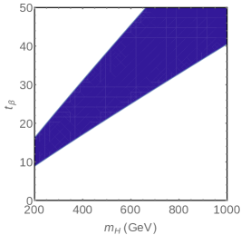
The allowed regions (tβvsmH)subscript𝑡𝛽𝑣𝑠subscript𝑚𝐻(t_{\beta}\,vs\,m_{H}) for case 1, 2a, 2b is presented in FIG.[11].
Refer to caption
Refer to caption
Refer to caption
Figure 11: Allowed regions for the cases: (a) case 1, (b) case 2a, (c) case 2b.

Case a) has the largest allowed region, since it allows for small Higgs masses with a small tβ10subscript𝑡𝛽10t_{\beta}\approx 10 through heavy Higgs of a large tβ50subscript𝑡𝛽50t_{\beta}\approx 50. While for case 2a we have a much more restricted parameter space, since small masses are allowed for a small range of tβ68subscript𝑡𝛽68t_{\beta}\approx 6-8 and the heaviest higgses are between tβ1216subscript𝑡𝛽1216t_{\beta}\approx 12-16. For the case 2b we also see a small allowed zone of parameter space, except that unlike the previous figure, slightly larger values of tβsubscript𝑡𝛽t_{\beta} are allowed.

  • tβsubscript𝑡𝛽t_{\beta} and mH±subscript𝑚superscript𝐻plus-or-minusm_{H^{\pm}}

For the charged heavy Higgs bosons we use the constraints IV.2.1-IV.2.2 to determine the allowed parameter space tβvsmH±subscript𝑡𝛽𝑣𝑠subscript𝑚superscript𝐻plus-or-minust_{\beta}\,vs\,m_{H^{\pm}}. Where we have used γ=0.5,(αβ)=π2,mH=500GeVformulae-sequence𝛾0.5formulae-sequence𝛼𝛽𝜋2subscript𝑚𝐻500𝐺𝑒𝑉\gamma=0{.}5,(\alpha-\beta)=\frac{\pi}{2},m_{H}=500\,GeV, mh0=125GeVsubscript𝑚superscript0125𝐺𝑒𝑉m_{h^{0}}=125\,GeV and θ1=π2,θ2=π4formulae-sequencesubscript𝜃1𝜋2subscript𝜃2𝜋4\theta_{1}=\frac{\pi}{2},\,\theta_{2}=\frac{\pi}{4}. The allowed regions (tβvsmH±)subscript𝑡𝛽𝑣𝑠subscript𝑚superscript𝐻plus-or-minus(t_{\beta}\,vs\,m_{H^{\pm}}) for case 1, 2a, 2b is presented in FIG.[12].

Refer to caption
Refer to caption
Refer to caption
Figure 12: Allowed regions for the cases: (a) case 1, (b) case 2a, (c) case 2b.

Constraints on the THDM must also satisfy electroweak precision data (EWPD). Thus, for our results to be reliable we verified that the parameter space regions explored are consistent with EWPD. In particular we found Higgs boson masses and tβsubscript𝑡𝛽t_{\beta} that satisfy radiative corrections to the W boson mass in the range of 100<mH<900GeV100subscript𝑚𝐻900𝐺𝑒𝑉100<m_{H}<900\,GeV (mH=mH0=mA0subscript𝑚𝐻subscript𝑚superscript𝐻0subscript𝑚superscript𝐴0m_{H}=m_{H^{0}}=m_{A^{0}}) and 1<tβ<401subscript𝑡𝛽401<t_{\beta}<40 for different values of mH±=300, 500, 800GeVsubscript𝑚superscript𝐻plus-or-minus300500800𝐺𝑒𝑉m_{H^{\pm}}=300,\,500,\,800\,GeV and mh0=125GeVsubscript𝑚superscript0125𝐺𝑒𝑉m_{h^{0}}=125\,GeV. Our results agree with the authors of [50]. A brief discution is included in App.VII.2.

V Results

In this section we show the results obtained for the magnetic and weak magnetic dipole moments in the framework of the THDM-III with four zero textures. In the previous section we presented the low energy processes involving either charged or neutral Higgs bosons and we explored what are the available allowed regions that satisfy the experimental bounds or measurements.

V.1 Muon anomalous magnetic dipole moment.

In FIG.[13] we show the contributions to aμsubscript𝑎𝜇a_{\mu} coming from the one loop diagrams in the context of THDM-III.

Refer to caption
Refer to caption
Refer to caption
Figure 13: New contribution of the THDM-III to aμsubscript𝑎𝜇a_{\mu} as function of Higgs mass (mH)subscript𝑚𝐻(m_{H}) and different values of tβsubscript𝑡𝛽t_{\beta} for reasonable values of free parameters of the model: γ=0.5,(αβ)=π2,mH=mH0=mA0,mH±=500GeVformulae-sequenceformulae-sequence𝛾0.5formulae-sequence𝛼𝛽𝜋2subscript𝑚𝐻subscript𝑚superscript𝐻0subscript𝑚superscript𝐴0subscript𝑚superscript𝐻plus-or-minus500𝐺𝑒𝑉\gamma=0.5,(\alpha-\beta)=\frac{\pi}{2},m_{H}=m_{H^{0}}=m_{A^{0}},m_{H^{\pm}}=500\,GeV and mh0=125GeVsubscript𝑚superscript0125𝐺𝑒𝑉m_{h^{0}}=125\,GeV for: (a) case 1, (b) case 2a, (c) case 2b. The parallel lines in all the plots correspond to allowed interval of the discrepancy ΔaμΔsubscript𝑎𝜇\Delta a_{\mu} between the prediction of the SM and experimental measurements with a 95% confidence level.

In each of the plots of FIG.[13] we notice that small masses mHsubscript𝑚𝐻m_{H} are allowed for small values of tβsubscript𝑡𝛽t_{\beta}, while heavier Higgs masses are only allowed for greater values of tβsubscript𝑡𝛽t_{\beta}.

V.2 Magnetic and weak magnetic dipole moments of the τ𝜏\tau.

Using the previously obtained parameter space, we show in FIG.[14] and FIG.[15], the THDM-III scalar contributions to the magnetic and weak magnetic dipole moments of the τ𝜏\tau.

Refer to caption
Refer to caption
Refer to caption
Figure 14: Plots of the scalar contributions to aτsubscript𝑎𝜏a_{\tau} in the THDM-III, (a) case 1, (b) case 2a, (c) case 2b.

from FIG.[14], we find that the contribution to aτsubscript𝑎𝜏a_{\tau} is contained between the current experimental value of [4],

0.052<aτ<0.058.0.052subscript𝑎𝜏0.058\displaystyle-0.052<a_{\tau}<0.058. (122)

We can see that the order of magnitude varies moderately for each of our cases. The contributions of case 1 are within the range 𝒪(108107)𝒪superscript108superscript107\mathcal{O}(10^{-8}-10^{-7}) while case 2a and 2b are 𝒪(108),𝒪(107)𝒪superscript108𝒪superscript107\mathcal{O}(10^{-8}),\,\mathcal{O}(10^{-7}), respectively. It is understandable because the three cases give similar contributions due to the structure of the Yukawa matrices we have considered.

On the other hand, in FIG.[15] shown planes aτWsuperscriptsubscript𝑎𝜏𝑊a_{\tau}^{W} vs mHsubscript𝑚𝐻m_{H}

Refer to caption
Refer to caption
Refer to caption
Figure 15: Plots of the scalar contributions to aτWsuperscriptsubscript𝑎𝜏𝑊a_{\tau}^{W} in the THDM-III, (a) case 1, (b) case 2a, (c) case 2b.

We note that the contributions of case 1 are 𝒪(109108)𝒪superscript109superscript108\mathcal{O}(10^{-9}-10^{-8}) while case 2a and 2b are 𝒪(1010109)𝒪(107)𝒪superscript1010superscript109𝒪superscript107\mathcal{O}(10^{-10}-10^{-9})-\mathcal{O}(10^{-7}), respectively.

VI Conclusions

We found that one loop level scalar contributions from the THDM-III with four zero textures can be a possible origin of the discrepancy ΔaμΔsubscript𝑎𝜇\Delta a_{\mu}. For small values of the mass of the heavy Higgs mHsubscript𝑚𝐻m_{H}, tβsubscript𝑡𝛽t_{\beta} is also small, and reciprocally, larger masses of mHsubscript𝑚𝐻m_{H} are permissible only for large tβsubscript𝑡𝛽t_{\beta}. Furthermore, using current low energy constraints and aμTHDMIIIsuperscriptsubscript𝑎𝜇𝑇𝐻𝐷𝑀𝐼𝐼𝐼a_{\mu}^{THDM-III}, we obtained the allowed parameter space of the Higgs boson masses and tβsubscript𝑡𝛽t_{\beta} which are also consistent with electroweak constraints. We determined that the magnetic dipole moment of the τ𝜏\tau lepton is of the order of 𝒪(108107)𝒪superscript108superscript107\mathcal{O}(10^{-8}-10^{-7}) and the weak magnetic of aτWsuperscriptsubscript𝑎𝜏𝑊a_{\tau}^{W} is of the order 𝒪(1010107)𝒪superscript1010superscript107\mathcal{O}(10^{-10}-10^{-7}). Of the three cases that we consider the dipole moments found in case 2b have the largest value for ali(W)superscriptsubscript𝑎subscript𝑙𝑖𝑊a_{l_{i}}^{(W)}.

Acknowledgements.
We acknowledge support from CONACYT (México). And appreciate the advice and discussions of this work with Gilberto Tavares-Velasco, Lorenzo Diaz-Cruz and Agustin Moyotl.

References

  • [1] G. Bennett et al. (Muon G-2 Collaboration), Phys.Rev.D73, 072003 (2006), arXiv:hep-ex/0602035.
  • [2] M. Jung and A. Pich, JHEP1404, 076 (2014) [arXiv:1308.6283 [hep-ph].
  • [3] D. Gomez-Dumm and G. Gonzalez-Sprinberg, Eur.Phys.J.C11, 293 (1999), arXiv:hep-ph/9905213 [hep-ph].
  • [4] J. Abdallah et al. [DELPHI Collaboration], Eur. Phys. J. C 35 (2004) 159.
  • [5] S. Eidelman and M. Passera, Mod.Phys.Lett. A22, 159 (2007), arXiv:hep-ph/0701260 [hep-ph].
  • [6] Bolaños, A. and Moyotl, A. and Tavares-Velasco, G., Phys. Rev. D89 2014, arxiv:1312.6860
  • [7] T. Ibrahim and P. Nath, Phys.Rev. D78 , 075013 (2008), arXiv:0806.3880 [hep-ph].
  • [8] A. Moyotl and G. Tavares-Velasco, Phys.Rev.D86, 013014 (2012), arXiv:1210.1994 [hep-ph]
  • [9] J. Bernabeu, G. Gonzalez-Sprinberg, M. Tung, and J. Vidal, Nucl.Phys.B436, 474 (1995), arXiv:hep-ph/9411289 [hep-ph]
  • [10] B. de Carlos and J. Moreno, Nucl.Phys. B519 , 101 (1998), arXiv:hep-ph/9707487 [hep-ph]; W. Hollik, J. I. Illana, S. Rigolin, and D. Stockinger, Phys.Lett. B416 , 345 (1998), arXiv:hep-ph/9707437 [hep-ph].
  • [11] A. Heister et al. (ALEPH Collaboration), Eur.Phys.J. C30, 291 (2003), arXiv:hep-ex/0209066.
  • [12] M. Laursen, M. A. Samuel, and A. Sen, Phys.Rev.D29, 2652 (1984).
  • [13] Qing-Jun Xu, Chao-Hsi Chang, arXiv:1410.1774v2 [hep-ph]
  • [14] Buras, Andrzej J. and Carlucci, Maria Valentina and Gori, Stefania and Isidori, Gino. JHEP,  10,  2010.
  • [15] T. P. Cheng and M. Sher, Phys. Rev. D 35, 3484 (1987).
  • [16] Honda, Mizue and Kaneko, Satoru and Tanimoto, Morimitsu, Phys. Lett. B593.  2004.
  • [17] Branco, G. C. and Emmanuel-Costa, D. and Simoes, C. Phys. Lett.,  B690,  2010.
  • [18] G. C. Branco, P. M. Ferreira, L. Lavoura, M. N. Rebelo, M. Sher, and J. P. Silva, Theory and phenomenology of two-Higgs-doublet models, Phys. Rept. 516(2012) 1 [arXiv:1106.0034 [hep-ph]].
  • [19] H. Nishiura, K. Matsuda and T. Fukuyama, PHYSICAL REVIEW D, VOLUME 60, 013006.
  • [20] J.L. Diaz-Cruz, R. Noriega-Papaqui and A. Rosado,
  • [21] G. C. Branco, D. Emmanuel-Costa and R. Gonzalez Felipe, Phys. Lett. B 477, 147 (2000) [hep-ph/9911418].
  • [22] M. Gomez-Bock and R. Noriega-Papaqui, J. Phys. G 32, 761 (2006) [hep-ph/0509353].
  • [23] J. F. Gunion, H. E. Haber, G. L. Kane and S. Dawson, “The Higgs Hunter’s Guide,” Front. Phys.  80, 1 (2000).
  • [24] D. Chang, W.-F. Chang, C.-H. Chou, and W.-Y. Keung, Phys.Rev. D 63, 091301(R)(2001).
  • [25] F. Larios, G- Tavares-Velasco, C.-P Yuan, Phys-Rev. D 64, 055004.
  • [26] OPAL Collaboration, G. Abbiendi et.al., Eur. Phys. J. C 18, 425 (2001).
  • [27] Dean Carmi, Adam Falkowski, Eric Kuflik, Tomer Volansky, Jure Zupan, 10.1007/JHEP10(2012)196, arXiv:1207.1718v3 [hep-ph].
  • [28] J. Abdallah et al. [DELPHI Collaboration], Eur. Phys. J. C 38 (2004) 1 [hep-ex/0410017].
  • [29] The OPAL Collaboration, Search for a low mass CP-odd Higgs boson in electron positron collisions with the OPAL detector at LEP2, Eur. Phys. J. C27 (2003), [hep-ex/0209068].
  • [30] M. Arroyo, J. L. Diaz-Cruz, E. Diaz and J. A Orduz-Ducuara, arXiv:1306.2343 [hep-ph]
  • [31] G. CVETIC, S. S. HWANG, and C. S. KIM, Int. J. Mod. Phys. A 14, 769 (1999). DOI: 10.1142/S0217751X99000385
  • [32] Zhi-zhong Xing, Zhen-hua Zhao. DOI:10.1016/j.nuclphysb.2015.05.027. arXiv:1501.06346v2 [hep-ph].
  • [33] P.M. Ferreira, R. Guedes, J.F. Gunion, H.E. Haber, M.O.P. Sampaio, R. Santos, The Wrong Sign limit in the 2HDM, arXiv:1410.1926 [hep-ph].
  • [34] A. Heister et al. (ALEPH Collaboration), Eur.Phys.J. C30, 291 (2003), arXiv:hep-ex/0209066 [hep-ex].
  • [35] V. Khachatryan et al., [CMS and LHCb Collaborations], arXiv:1411.4413 [hep-ex].
  • [36] C. Bobeth et al. , Phys. Rev. Lett. 112 (2014) 101801.
  • [37] A. Dedes and A. Pilaftsis, Phys. Rev. D 67, 015012 (2003) [hep-ph/0209306].
  • [38] Crivellin A Kokulu A and Greub C 2013 Flavor-phenomenology of two-Higgs-doublet models with generic Yukawa structure,” Phys. Rev.D879, 094031 [arXiv:1303.5877 [hep-ph]]
  • [39] J. Adam et al. [MEG Collaboration], Phys. Rev. Lett. 110, no. 20, 201801 (2013) [arXiv:1303.0754 [hep-ex]].
  • [40] B. Aubert et al. [BaBar Collaboration], Phys. Rev. Lett. 104, 021802 (2010) [arXiv:0908.2381 [hep-ex]].
  • [41] K. Hayasaka et al. [Belle Collaboration], Phys. Lett. B 666, 16 (2008) [arXiv:0705.0650 [hep-ex]].
  • [42] Dedes, Athanasios and Pilaftsis, Apostolos, Phys. Rev., D67, 2003, 015012, 10.1103/PhysRevD.67.015012.
  • [43] Y-F. Zhou, J.Phys.G30:783-792,2004.
  • [44] Olive, K. A. and others, Review of Particle Physics, Particle Data Group, Chin. Phys., C38, 2014.
  • [45] F. Borzumati and C. Greub, Phys. Rev. D 58, 074004 (1998) [hep-ph/9802391].
  • [46] P. Ciafaloni, A. Romanino and A. Strumia, Nucl. Phys. B 524, 361 (1998) [hep-ph/9710312].
  • [47] Lees, J. P. et al. Phys. Rev.D88, 2013, 7, 072012.
  • [48] A. Crivellin, C. Greub and A. Kokulu, Phys. Rev. D 86, 054014 (2012) [arXiv:1206.2634 [hep-ph].
  • [49] V. Khachatryan et al. [CMS Collaboration], arXiv:1502.07400 [hep-ex].
  • [50] Alessandro Broggio, Eung Jin Chun, Massimo Passera, Ketan M. Patel, Sudhir K. Vempati, arXiv:1409.3199v1 [hep-ph].
  • [51] David Lopez-Val and Joan Sola, arXiv:1211.0311v3.

VII Appendix

VII.1 Yukawa elements for Case 1

Y~21subscript~𝑌21\displaystyle\widetilde{Y}_{21} =\displaystyle= ei(θ1+θ2)γm1m2(γm2+m2m3)(m1+m2)(m1+m3)(γm2m3)superscript𝑒𝑖subscript𝜃1subscript𝜃2𝛾subscript𝑚1subscript𝑚2𝛾subscript𝑚2subscript𝑚2subscript𝑚3subscript𝑚1subscript𝑚2subscript𝑚1subscript𝑚3𝛾subscript𝑚2subscript𝑚3\displaystyle e^{-i\left(\theta_{1}+\theta_{2}\right)}\sqrt{\frac{\gamma m_{1}m_{2}\left(\gamma m_{2}+m_{2}-m_{3}\right)}{\left(m_{1}+m_{2}\right)\left(m_{1}+m_{3}\right)\left(\gamma m_{2}-m_{3}\right)}}
×\displaystyle\times (ei(θ1+θ2)γm22(γm2+m1+m3)(m1+m2)(m2m3)(γm2m3)(γm2m3)\displaystyle\left(e^{i\left(\theta_{1}+\theta_{2}\right)}\sqrt{\frac{\gamma m_{2}^{2}\left(-\gamma m_{2}+m_{1}+m_{3}\right)}{\left(m_{1}+m_{2}\right)\left(m_{2}-m_{3}\right)\left(\gamma m_{2}-m_{3}\right)}}\left(\gamma m_{2}-m_{3}\right)\right.
+\displaystyle+ eiθ1θ2m2(γm2+m2m3)(m1+m2)(m2m3)superscript𝑒𝑖subscript𝜃1subscript𝜃2subscript𝑚2𝛾subscript𝑚2subscript𝑚2subscript𝑚3subscript𝑚1subscript𝑚2subscript𝑚2subscript𝑚3\displaystyle e^{i\theta_{1}\theta_{2}}\sqrt{\frac{m_{2}\left(\gamma m_{2}+m_{2}-m_{3}\right)}{\left(m_{1}+m_{2}\right)\left(m_{2}-m_{3}\right)}}
×\displaystyle\times γm2(γm2+m2m3)(γm2+m1+m3)γm2m3)\displaystyle\left.\sqrt{\frac{\gamma m_{2}\left(\gamma m_{2}+m_{2}-m_{3}\right)\left(-\gamma m_{2}+m_{1}+m_{3}\right)}{\gamma m_{2}-m_{3}}}\right)
+\displaystyle+ eiθ1θ2m1(γm2+m1+m3)(m1+m2)(m1+m3)superscript𝑒𝑖subscript𝜃1subscript𝜃2subscript𝑚1𝛾subscript𝑚2subscript𝑚1subscript𝑚3subscript𝑚1subscript𝑚2subscript𝑚1subscript𝑚3\displaystyle e^{-i\theta_{1}\theta_{2}}\sqrt{\frac{m_{1}\left(-\gamma m_{2}+m_{1}+m_{3}\right)}{\left(m_{1}+m_{2}\right)\left(m_{1}+m_{3}\right)}}
×\displaystyle\times (eiθ1θ2m2(γm2+m2m3)(m1+m2)(m2m3)(γm2m1+m2)\displaystyle\left(-e^{i\theta_{1}\theta_{2}}\sqrt{\frac{m_{2}\left(\gamma m_{2}+m_{2}-m_{3}\right)}{\left(m_{1}+m_{2}\right)\left(m_{2}-m_{3}\right)}}\left(\gamma m_{2}-m_{1}+m_{2}\right)\right.
\displaystyle- ei(θ2θ1+θ1+θ2)m1m2m3γm2m3superscript𝑒𝑖subscript𝜃2subscript𝜃1subscript𝜃1subscript𝜃2subscript𝑚1subscript𝑚2subscript𝑚3𝛾subscript𝑚2subscript𝑚3\displaystyle e^{i\left(\theta_{2}\theta_{1}+\theta_{1}+\theta_{2}\right)}\sqrt{-\frac{m_{1}m_{2}m_{3}}{\gamma m_{2}-m_{3}}}
×\displaystyle\times m1m3(γm2+m2m3)(m1+m2)(m2m3)(γm2m3)+ei(θ1+θ2)subscript𝑚1subscript𝑚3𝛾subscript𝑚2subscript𝑚2subscript𝑚3subscript𝑚1subscript𝑚2subscript𝑚2subscript𝑚3𝛾subscript𝑚2subscript𝑚3superscript𝑒𝑖subscript𝜃1subscript𝜃2\displaystyle\sqrt{-\frac{m_{1}m_{3}\left(\gamma m_{2}+m_{2}-m_{3}\right)}{\left(m_{1}+m_{2}\right)\left(m_{2}-m_{3}\right)\left(\gamma m_{2}-m_{3}\right)}}+e^{i\left(\theta_{1}+\theta_{2}\right)}
×\displaystyle\times γm22(γm2+m1+m3)(m1+m2)(m2m3)(γm2m3)𝛾superscriptsubscript𝑚22𝛾subscript𝑚2subscript𝑚1subscript𝑚3subscript𝑚1subscript𝑚2subscript𝑚2subscript𝑚3𝛾subscript𝑚2subscript𝑚3\displaystyle\sqrt{\frac{\gamma m_{2}^{2}\left(-\gamma m_{2}+m_{1}+m_{3}\right)}{\left(m_{1}+m_{2}\right)\left(m_{2}-m_{3}\right)\left(\gamma m_{2}-m_{3}\right)}}
×\displaystyle\times γm2(γm2+m2m3)(γm2+m1+m3)γm2m3)\displaystyle\left.\sqrt{\frac{\gamma m_{2}\left(\gamma m_{2}+m_{2}-m_{3}\right)\left(-\gamma m_{2}+m_{1}+m_{3}\right)}{\gamma m_{2}-m_{3}}}\right)
+\displaystyle+ ei(θ1+θ2)m2(γm2+m2m3)(m1+m2)(m2m3)m1m2m3γm2m3superscript𝑒𝑖subscript𝜃1subscript𝜃2subscript𝑚2𝛾subscript𝑚2subscript𝑚2subscript𝑚3subscript𝑚1subscript𝑚2subscript𝑚2subscript𝑚3subscript𝑚1subscript𝑚2subscript𝑚3𝛾subscript𝑚2subscript𝑚3\displaystyle e^{-i\left(\theta_{1}+\theta_{2}\right)}\sqrt{\frac{m_{2}\left(\gamma m_{2}+m_{2}-m_{3}\right)}{\left(m_{1}+m_{2}\right)\left(m_{2}-m_{3}\right)}}\sqrt{-\frac{m_{1}m_{2}m_{3}}{\gamma m_{2}-m_{3}}}
×\displaystyle\times m2m3(γm2m1m3)(m1+m2)(m1+m3)(γm2m3)subscript𝑚2subscript𝑚3𝛾subscript𝑚2subscript𝑚1subscript𝑚3subscript𝑚1subscript𝑚2subscript𝑚1subscript𝑚3𝛾subscript𝑚2subscript𝑚3\displaystyle\sqrt{\frac{m_{2}m_{3}\left(\gamma m_{2}-m_{1}-m_{3}\right)}{\left(m_{1}+m_{2}\right)\left(m_{1}+m_{3}\right)\left(\gamma m_{2}-m_{3}\right)}}
Y~22subscript~𝑌22\displaystyle\widetilde{Y}_{22} =\displaystyle= 2m2(γm2+m2m3)(m1+m2)(m2m3)(m1m2m3γm2m3m1m3(γm2+m2m3)(m1+m2)(m2m3)(γm2m3)\displaystyle 2\sqrt{\frac{m_{2}\left(\gamma m_{2}+m_{2}-m_{3}\right)}{\left(m_{1}+m_{2}\right)\left(m_{2}-m_{3}\right)}}\left(\sqrt{-\frac{m_{1}m_{2}m_{3}}{\gamma m_{2}-m_{3}}}\sqrt{-\frac{m_{1}m_{3}\left(\gamma m_{2}+m_{2}-m_{3}\right)}{\left(m_{1}+m_{2}\right)\left(m_{2}-m_{3}\right)\left(\gamma m_{2}-m_{3}\right)}}\right.
×\displaystyle\times cos(θ1+θ2)γm22(γm2+m1+m3)(m1+m2)(m2m3)(γm2m3)subscript𝜃1subscript𝜃2𝛾superscriptsubscript𝑚22𝛾subscript𝑚2subscript𝑚1subscript𝑚3subscript𝑚1subscript𝑚2subscript𝑚2subscript𝑚3𝛾subscript𝑚2subscript𝑚3\displaystyle\cos\left(\theta_{1}+\theta_{2}\right)-\sqrt{\frac{\gamma m_{2}^{2}\left(-\gamma m_{2}+m_{1}+m_{3}\right)}{\left(m_{1}+m_{2}\right)\left(m_{2}-m_{3}\right)\left(\gamma m_{2}-m_{3}\right)}}
×\displaystyle\times γm2(γm2+m2m3)(γm2+m1+m3)γm2m3cos(θ2θ1+θ1+θ2))\displaystyle\left.\sqrt{\frac{\gamma m_{2}\left(\gamma m_{2}+m_{2}-m_{3}\right)\left(-\gamma m_{2}+m_{1}+m_{3}\right)}{\gamma m_{2}-m_{3}}}\cos\left(-\theta_{2}\theta_{1}+\theta_{1}+\theta_{2}\right)\right)
+\displaystyle+ m2(m2((2γ1)m1+2γ(γ+1)m2+m2)+m3(m1(2γ+1)m2))(m1+m2)(m2m3)subscript𝑚2subscript𝑚22𝛾1subscript𝑚12𝛾𝛾1subscript𝑚2subscript𝑚2subscript𝑚3subscript𝑚12𝛾1subscript𝑚2subscript𝑚1subscript𝑚2subscript𝑚2subscript𝑚3\displaystyle\frac{m_{2}\left(m_{2}\left((-2\gamma-1)m_{1}+2\gamma(\gamma+1)m_{2}+m_{2}\right)+m_{3}\left(m_{1}-(2\gamma+1)m_{2}\right)\right)}{\left(m_{1}+m_{2}\right)\left(m_{2}-m_{3}\right)}
Y~23subscript~𝑌23\displaystyle\widetilde{Y}_{23} =\displaystyle= ei(θ1+θ2)m3(γm2+m2m3)(γm2+m1+m3)(m2m3)(m1+m3)(γm2m3)superscript𝑒𝑖subscript𝜃1subscript𝜃2subscript𝑚3𝛾subscript𝑚2subscript𝑚2subscript𝑚3𝛾subscript𝑚2subscript𝑚1subscript𝑚3subscript𝑚2subscript𝑚3subscript𝑚1subscript𝑚3𝛾subscript𝑚2subscript𝑚3\displaystyle e^{-i\left(\theta_{1}+\theta_{2}\right)}\sqrt{-\frac{m_{3}\left(\gamma m_{2}+m_{2}-m_{3}\right)\left(-\gamma m_{2}+m_{1}+m_{3}\right)}{\left(m_{2}-m_{3}\right)\left(m_{1}+m_{3}\right)\left(\gamma m_{2}-m_{3}\right)}}
×\displaystyle\times (ei(θ1+θ2)γm22(γm2+m1+m3)(m1+m2)(m2m3)(γm2m3)\displaystyle\left(e^{i\left(\theta_{1}+\theta_{2}\right)}\sqrt{\frac{\gamma m_{2}^{2}\left(-\gamma m_{2}+m_{1}+m_{3}\right)}{\left(m_{1}+m_{2}\right)\left(m_{2}-m_{3}\right)\left(\gamma m_{2}-m_{3}\right)}}\right.
×\displaystyle\times (γm2m3)+eiθ1θ2m2(γm2+m2m3)(m1+m2)(m2m3)𝛾subscript𝑚2subscript𝑚3superscript𝑒𝑖subscript𝜃1subscript𝜃2subscript𝑚2𝛾subscript𝑚2subscript𝑚2subscript𝑚3subscript𝑚1subscript𝑚2subscript𝑚2subscript𝑚3\displaystyle\left(\gamma m_{2}-m_{3}\right)+e^{i\theta_{1}\theta_{2}}\sqrt{\frac{m_{2}\left(\gamma m_{2}+m_{2}-m_{3}\right)}{\left(m_{1}+m_{2}\right)\left(m_{2}-m_{3}\right)}}
×\displaystyle\times γm2(γm2+m2m3)(γm2+m1+m3)γm2m3)\displaystyle\left.\sqrt{\frac{\gamma m_{2}\left(\gamma m_{2}+m_{2}-m_{3}\right)\left(-\gamma m_{2}+m_{1}+m_{3}\right)}{\gamma m_{2}-m_{3}}}\right)
+\displaystyle+ eiθ1θ2γm2m3(m2m3)(m1+m3)(eiθ1θ2m2(γm2+m2m3)(m1+m2)(m2m3)\displaystyle e^{-i\theta_{1}\theta_{2}}\sqrt{-\frac{\gamma m_{2}m_{3}}{\left(m_{2}-m_{3}\right)\left(m_{1}+m_{3}\right)}}\left(e^{i\theta_{1}\theta_{2}}\sqrt{\frac{m_{2}\left(\gamma m_{2}+m_{2}-m_{3}\right)}{\left(m_{1}+m_{2}\right)\left(m_{2}-m_{3}\right)}}\right.
×\displaystyle\times (γm2m1+m2)+ei(θ2θ1+θ1+θ2)m1m2m3γm2m3𝛾subscript𝑚2subscript𝑚1subscript𝑚2superscript𝑒𝑖subscript𝜃2subscript𝜃1subscript𝜃1subscript𝜃2subscript𝑚1subscript𝑚2subscript𝑚3𝛾subscript𝑚2subscript𝑚3\displaystyle\left(\gamma m_{2}-m_{1}+m_{2}\right)+e^{i\left(\theta_{2}\theta_{1}+\theta_{1}+\theta_{2}\right)}\sqrt{-\frac{m_{1}m_{2}m_{3}}{\gamma m_{2}-m_{3}}}
×\displaystyle\times m1m3(γm2+m2m3)(m1+m2)(m2m3)(γm2m3)subscript𝑚1subscript𝑚3𝛾subscript𝑚2subscript𝑚2subscript𝑚3subscript𝑚1subscript𝑚2subscript𝑚2subscript𝑚3𝛾subscript𝑚2subscript𝑚3\displaystyle\sqrt{-\frac{m_{1}m_{3}\left(\gamma m_{2}+m_{2}-m_{3}\right)}{\left(m_{1}+m_{2}\right)\left(m_{2}-m_{3}\right)\left(\gamma m_{2}-m_{3}\right)}}
\displaystyle- ei(θ1+θ2)γm22(γm2+m1+m3)(m1+m2)(m2m3)(γm2m3)superscript𝑒𝑖subscript𝜃1subscript𝜃2𝛾superscriptsubscript𝑚22𝛾subscript𝑚2subscript𝑚1subscript𝑚3subscript𝑚1subscript𝑚2subscript𝑚2subscript𝑚3𝛾subscript𝑚2subscript𝑚3\displaystyle e^{i\left(\theta_{1}+\theta_{2}\right)}\sqrt{\frac{\gamma m_{2}^{2}\left(-\gamma m_{2}+m_{1}+m_{3}\right)}{\left(m_{1}+m_{2}\right)\left(m_{2}-m_{3}\right)\left(\gamma m_{2}-m_{3}\right)}}
×\displaystyle\times γm2(γm2+m2m3)(γm2+m1+m3)γm2m3)\displaystyle\left.\sqrt{\frac{\gamma m_{2}\left(\gamma m_{2}+m_{2}-m_{3}\right)\left(-\gamma m_{2}+m_{1}+m_{3}\right)}{\gamma m_{2}-m_{3}}}\right)
+\displaystyle+ ei(θ1+θ2)m2(γm2+m2m3)(m1+m2)(m2m3)m1m2m3γm2m3superscript𝑒𝑖subscript𝜃1subscript𝜃2subscript𝑚2𝛾subscript𝑚2subscript𝑚2subscript𝑚3subscript𝑚1subscript𝑚2subscript𝑚2subscript𝑚3subscript𝑚1subscript𝑚2subscript𝑚3𝛾subscript𝑚2subscript𝑚3\displaystyle e^{-i\left(\theta_{1}+\theta_{2}\right)}\sqrt{\frac{m_{2}\left(\gamma m_{2}+m_{2}-m_{3}\right)}{\left(m_{1}+m_{2}\right)\left(m_{2}-m_{3}\right)}}\sqrt{-\frac{m_{1}m_{2}m_{3}}{\gamma m_{2}-m_{3}}}
×\displaystyle\times γm1m22(m2m3)(m1+m3)(γm2m3)𝛾subscript𝑚1superscriptsubscript𝑚22subscript𝑚2subscript𝑚3subscript𝑚1subscript𝑚3𝛾subscript𝑚2subscript𝑚3\displaystyle\sqrt{\frac{\gamma m_{1}m_{2}^{2}}{\left(m_{2}-m_{3}\right)\left(m_{1}+m_{3}\right)\left(\gamma m_{2}-m_{3}\right)}}
Y~31subscript~𝑌31\displaystyle\widetilde{Y}_{31} =\displaystyle= ei(θ1+θ2)γm1m2(γm2+m2m3)(m1+m2)(m1+m3)(γm2m3)(ei(θ1+θ2)\displaystyle e^{-i\left(\theta_{1}+\theta_{2}\right)}\sqrt{\frac{\gamma m_{1}m_{2}\left(\gamma m_{2}+m_{2}-m_{3}\right)}{\left(m_{1}+m_{2}\right)\left(m_{1}+m_{3}\right)\left(\gamma m_{2}-m_{3}\right)}}\left(e^{i\left(\theta_{1}+\theta_{2}\right)}\right.
×\displaystyle\times m3(γm2+m2m3)(γm2+m1+m3)(m2m3)(m1+m3)(γm2m3)(m3γm2)subscript𝑚3𝛾subscript𝑚2subscript𝑚2subscript𝑚3𝛾subscript𝑚2subscript𝑚1subscript𝑚3subscript𝑚2subscript𝑚3subscript𝑚1subscript𝑚3𝛾subscript𝑚2subscript𝑚3subscript𝑚3𝛾subscript𝑚2\displaystyle\sqrt{-\frac{m_{3}\left(\gamma m_{2}+m_{2}-m_{3}\right)\left(-\gamma m_{2}+m_{1}+m_{3}\right)}{\left(m_{2}-m_{3}\right)\left(m_{1}+m_{3}\right)\left(\gamma m_{2}-m_{3}\right)}}\left(m_{3}-\gamma m_{2}\right)
+\displaystyle+ eiθ1θ2γm2m3(m2m3)(m1+m3)superscript𝑒𝑖subscript𝜃1subscript𝜃2𝛾subscript𝑚2subscript𝑚3subscript𝑚2subscript𝑚3subscript𝑚1subscript𝑚3\displaystyle e^{i\theta_{1}\theta_{2}}\sqrt{-\frac{\gamma m_{2}m_{3}}{\left(m_{2}-m_{3}\right)\left(m_{1}+m_{3}\right)}}
×\displaystyle\times γm2(γm2+m2m3)(γm2+m1+m3)γm2m3)\displaystyle\left.\sqrt{\frac{\gamma m_{2}\left(\gamma m_{2}+m_{2}-m_{3}\right)\left(-\gamma m_{2}+m_{1}+m_{3}\right)}{\gamma m_{2}-m_{3}}}\right)
+\displaystyle+ eiθ1θ2m1(γm2+m1+m3)(m1+m2)(m1+m3)(eiθ1θ2γm2m3(m2m3)(m1+m3)\displaystyle e^{-i\theta_{1}\theta_{2}}\sqrt{\frac{m_{1}\left(-\gamma m_{2}+m_{1}+m_{3}\right)}{\left(m_{1}+m_{2}\right)\left(m_{1}+m_{3}\right)}}\left(-e^{i\theta_{1}\theta_{2}}\sqrt{-\frac{\gamma m_{2}m_{3}}{\left(m_{2}-m_{3}\right)\left(m_{1}+m_{3}\right)}}\right.
×\displaystyle\times (γm2m1+m2)ei(θ2θ1+θ1+θ2)m1m2m3γm2m3𝛾subscript𝑚2subscript𝑚1subscript𝑚2superscript𝑒𝑖subscript𝜃2subscript𝜃1subscript𝜃1subscript𝜃2subscript𝑚1subscript𝑚2subscript𝑚3𝛾subscript𝑚2subscript𝑚3\displaystyle\left(\gamma m_{2}-m_{1}+m_{2}\right)-e^{i\left(\theta_{2}\theta_{1}+\theta_{1}+\theta_{2}\right)}\sqrt{-\frac{m_{1}m_{2}m_{3}}{\gamma m_{2}-m_{3}}}
×\displaystyle\times γm1m22(m2m3)(m1+m3)(γm2m3)𝛾subscript𝑚1superscriptsubscript𝑚22subscript𝑚2subscript𝑚3subscript𝑚1subscript𝑚3𝛾subscript𝑚2subscript𝑚3\displaystyle\sqrt{\frac{\gamma m_{1}m_{2}^{2}}{\left(m_{2}-m_{3}\right)\left(m_{1}+m_{3}\right)\left(\gamma m_{2}-m_{3}\right)}}
\displaystyle- ei(θ1+θ2)γm2(γm2+m2m3)(γm2+m1+m3)γm2m3superscript𝑒𝑖subscript𝜃1subscript𝜃2𝛾subscript𝑚2𝛾subscript𝑚2subscript𝑚2subscript𝑚3𝛾subscript𝑚2subscript𝑚1subscript𝑚3𝛾subscript𝑚2subscript𝑚3\displaystyle e^{i\left(\theta_{1}+\theta_{2}\right)}\sqrt{\frac{\gamma m_{2}\left(\gamma m_{2}+m_{2}-m_{3}\right)\left(-\gamma m_{2}+m_{1}+m_{3}\right)}{\gamma m_{2}-m_{3}}}
×\displaystyle\times m3(γm2+m2m3)(γm2+m1+m3)(m2m3)(m1+m3)(γm2m3))\displaystyle\left.\sqrt{-\frac{m_{3}\left(\gamma m_{2}+m_{2}-m_{3}\right)\left(-\gamma m_{2}+m_{1}+m_{3}\right)}{\left(m_{2}-m_{3}\right)\left(m_{1}+m_{3}\right)\left(\gamma m_{2}-m_{3}\right)}}\right)
+\displaystyle+ ei(θ1+θ2)m1m2m3γm2m3γm2m3(m2m3)(m1+m3)superscript𝑒𝑖subscript𝜃1subscript𝜃2subscript𝑚1subscript𝑚2subscript𝑚3𝛾subscript𝑚2subscript𝑚3𝛾subscript𝑚2subscript𝑚3subscript𝑚2subscript𝑚3subscript𝑚1subscript𝑚3\displaystyle e^{-i\left(\theta_{1}+\theta_{2}\right)}\sqrt{-\frac{m_{1}m_{2}m_{3}}{\gamma m_{2}-m_{3}}}\sqrt{-\frac{\gamma m_{2}m_{3}}{\left(m_{2}-m_{3}\right)\left(m_{1}+m_{3}\right)}}
×\displaystyle\times m2m3(γm2m1m3)(m1+m2)(m1+m3)(γm2m3)subscript𝑚2subscript𝑚3𝛾subscript𝑚2subscript𝑚1subscript𝑚3subscript𝑚1subscript𝑚2subscript𝑚1subscript𝑚3𝛾subscript𝑚2subscript𝑚3\displaystyle\sqrt{\frac{m_{2}m_{3}\left(\gamma m_{2}-m_{1}-m_{3}\right)}{\left(m_{1}+m_{2}\right)\left(m_{1}+m_{3}\right)\left(\gamma m_{2}-m_{3}\right)}}
Y~32subscript~𝑌32\displaystyle\widetilde{Y}_{32} =\displaystyle= eiθ1θ2γm22(γm2+m1+m3)(m1+m2)(m2m3)(γm2m3)(eiθ1θ2\displaystyle-e^{i\theta_{1}\theta_{2}}\sqrt{\frac{\gamma m_{2}^{2}\left(-\gamma m_{2}+m_{1}+m_{3}\right)}{\left(m_{1}+m_{2}\right)\left(m_{2}-m_{3}\right)\left(\gamma m_{2}-m_{3}\right)}}\left(e^{-i\theta_{1}\theta_{2}}\right.
×\displaystyle\times m3(γm2+m2m3)(γm2+m1+m3)(m2m3)(m1+m3)(γm2m3)(m3γm2)subscript𝑚3𝛾subscript𝑚2subscript𝑚2subscript𝑚3𝛾subscript𝑚2subscript𝑚1subscript𝑚3subscript𝑚2subscript𝑚3subscript𝑚1subscript𝑚3𝛾subscript𝑚2subscript𝑚3subscript𝑚3𝛾subscript𝑚2\displaystyle\sqrt{-\frac{m_{3}\left(\gamma m_{2}+m_{2}-m_{3}\right)\left(-\gamma m_{2}+m_{1}+m_{3}\right)}{\left(m_{2}-m_{3}\right)\left(m_{1}+m_{3}\right)\left(\gamma m_{2}-m_{3}\right)}}\left(m_{3}-\gamma m_{2}\right)
+\displaystyle+ ei(θ1+θ2)γm2m3(m2m3)(m1+m3)superscript𝑒𝑖subscript𝜃1subscript𝜃2𝛾subscript𝑚2subscript𝑚3subscript𝑚2subscript𝑚3subscript𝑚1subscript𝑚3\displaystyle e^{-i\left(\theta_{1}+\theta_{2}\right)}\sqrt{-\frac{\gamma m_{2}m_{3}}{\left(m_{2}-m_{3}\right)\left(m_{1}+m_{3}\right)}}
×\displaystyle\times γm2(γm2+m2m3)(γm2+m1+m3)γm2m3)\displaystyle\left.\sqrt{\frac{\gamma m_{2}\left(\gamma m_{2}+m_{2}-m_{3}\right)\left(-\gamma m_{2}+m_{1}+m_{3}\right)}{\gamma m_{2}-m_{3}}}\right)
+\displaystyle+ eiθ1θ2m2(γm2+m2m3)(m1+m2)(m2m3)(eiθ1θ2γm2m3(m2m3)(m1+m3)\displaystyle e^{-i\theta_{1}\theta_{2}}\sqrt{\frac{m_{2}\left(\gamma m_{2}+m_{2}-m_{3}\right)}{\left(m_{1}+m_{2}\right)\left(m_{2}-m_{3}\right)}}\left(e^{i\theta_{1}\theta_{2}}\sqrt{-\frac{\gamma m_{2}m_{3}}{\left(m_{2}-m_{3}\right)\left(m_{1}+m_{3}\right)}}\right.
×\displaystyle\times (γm2m1+m2)+ei(θ2θ1+θ1+θ2)m1m2m3γm2m3𝛾subscript𝑚2subscript𝑚1subscript𝑚2superscript𝑒𝑖subscript𝜃2subscript𝜃1subscript𝜃1subscript𝜃2subscript𝑚1subscript𝑚2subscript𝑚3𝛾subscript𝑚2subscript𝑚3\displaystyle\left(\gamma m_{2}-m_{1}+m_{2}\right)+e^{i\left(\theta_{2}\theta_{1}+\theta_{1}+\theta_{2}\right)}\sqrt{-\frac{m_{1}m_{2}m_{3}}{\gamma m_{2}-m_{3}}}
×\displaystyle\times γm1m22(m2m3)(m1+m3)(γm2m3)𝛾subscript𝑚1superscriptsubscript𝑚22subscript𝑚2subscript𝑚3subscript𝑚1subscript𝑚3𝛾subscript𝑚2subscript𝑚3\displaystyle\sqrt{\frac{\gamma m_{1}m_{2}^{2}}{\left(m_{2}-m_{3}\right)\left(m_{1}+m_{3}\right)\left(\gamma m_{2}-m_{3}\right)}}
+\displaystyle+ ei(θ1+θ2)γm2(γm2+m2m3)(γm2+m1+m3)γm2m3superscript𝑒𝑖subscript𝜃1subscript𝜃2𝛾subscript𝑚2𝛾subscript𝑚2subscript𝑚2subscript𝑚3𝛾subscript𝑚2subscript𝑚1subscript𝑚3𝛾subscript𝑚2subscript𝑚3\displaystyle e^{i\left(\theta_{1}+\theta_{2}\right)}\sqrt{\frac{\gamma m_{2}\left(\gamma m_{2}+m_{2}-m_{3}\right)\left(-\gamma m_{2}+m_{1}+m_{3}\right)}{\gamma m_{2}-m_{3}}}
×\displaystyle\times m3(γm2+m2m3)(γm2+m1+m3)(m2m3)(m1+m3)(γm2m3))\displaystyle\left.\sqrt{-\frac{m_{3}\left(\gamma m_{2}+m_{2}-m_{3}\right)\left(-\gamma m_{2}+m_{1}+m_{3}\right)}{\left(m_{2}-m_{3}\right)\left(m_{1}+m_{3}\right)\left(\gamma m_{2}-m_{3}\right)}}\right)
+\displaystyle+ ei(θ1+θ2)m1m2m3γm2m3m1m3(γm2+m2m3)(m1+m2)(m2m3)(γm2m3)superscript𝑒𝑖subscript𝜃1subscript𝜃2subscript𝑚1subscript𝑚2subscript𝑚3𝛾subscript𝑚2subscript𝑚3subscript𝑚1subscript𝑚3𝛾subscript𝑚2subscript𝑚2subscript𝑚3subscript𝑚1subscript𝑚2subscript𝑚2subscript𝑚3𝛾subscript𝑚2subscript𝑚3\displaystyle e^{-i\left(\theta_{1}+\theta_{2}\right)}\sqrt{-\frac{m_{1}m_{2}m_{3}}{\gamma m_{2}-m_{3}}}\sqrt{-\frac{m_{1}m_{3}\left(\gamma m_{2}+m_{2}-m_{3}\right)}{\left(m_{1}+m_{2}\right)\left(m_{2}-m_{3}\right)\left(\gamma m_{2}-m_{3}\right)}}
×\displaystyle\times γm2m3(m2m3)(m1+m3)𝛾subscript𝑚2subscript𝑚3subscript𝑚2subscript𝑚3subscript𝑚1subscript𝑚3\displaystyle\sqrt{-\frac{\gamma m_{2}m_{3}}{\left(m_{2}-m_{3}\right)\left(m_{1}+m_{3}\right)}}
Y~33subscript~𝑌33\displaystyle\widetilde{Y}_{33} =\displaystyle= 2γm2m3(m2m3)(m1+m3)(m1m2m3γm2m3\displaystyle 2\sqrt{-\frac{\gamma m_{2}m_{3}}{\left(m_{2}-m_{3}\right)\left(m_{1}+m_{3}\right)}}\left(\sqrt{-\frac{m_{1}m_{2}m_{3}}{\gamma m_{2}-m_{3}}}\right.
×\displaystyle\times γm1m22(m2m3)(m1+m3)(γm2m3)cos(θ1+θ2)𝛾subscript𝑚1superscriptsubscript𝑚22subscript𝑚2subscript𝑚3subscript𝑚1subscript𝑚3𝛾subscript𝑚2subscript𝑚3subscript𝜃1subscript𝜃2\displaystyle\sqrt{\frac{\gamma m_{1}m_{2}^{2}}{\left(m_{2}-m_{3}\right)\left(m_{1}+m_{3}\right)\left(\gamma m_{2}-m_{3}\right)}}\cos\left(\theta_{1}+\theta_{2}\right)
+\displaystyle+ γm2(γm2+m2m3)(γm2+m1+m3)γm2m3𝛾subscript𝑚2𝛾subscript𝑚2subscript𝑚2subscript𝑚3𝛾subscript𝑚2subscript𝑚1subscript𝑚3𝛾subscript𝑚2subscript𝑚3\displaystyle\sqrt{\frac{\gamma m_{2}\left(\gamma m_{2}+m_{2}-m_{3}\right)\left(-\gamma m_{2}+m_{1}+m_{3}\right)}{\gamma m_{2}-m_{3}}}
×\displaystyle\times m3(γm2+m2m3)(γm2+m1+m3)(m2m3)(m1+m3)(γm2m3)cos(θ2θ1+θ1+θ2))\displaystyle\left.\sqrt{-\frac{m_{3}\left(\gamma m_{2}+m_{2}-m_{3}\right)\left(-\gamma m_{2}+m_{1}+m_{3}\right)}{\left(m_{2}-m_{3}\right)\left(m_{1}+m_{3}\right)\left(\gamma m_{2}-m_{3}\right)}}\cos\left(-\theta_{2}\theta_{1}+\theta_{1}+\theta_{2}\right)\right)
+\displaystyle+ m3(m3(2γm2m1+m2)+m2(2γm12γ(γ+1)m2+m1)m32)(m2m3)(m1+m3)subscript𝑚3subscript𝑚32𝛾subscript𝑚2subscript𝑚1subscript𝑚2subscript𝑚22𝛾subscript𝑚12𝛾𝛾1subscript𝑚2subscript𝑚1superscriptsubscript𝑚32subscript𝑚2subscript𝑚3subscript𝑚1subscript𝑚3\displaystyle\frac{m_{3}\left(m_{3}\left(2\gamma m_{2}-m_{1}+m_{2}\right)+m_{2}\left(2\gamma m_{1}-2\gamma(\gamma+1)m_{2}+m_{1}\right)-m_{3}^{2}\right)}{\left(m_{2}-m_{3}\right)\left(m_{1}+m_{3}\right)}

VII.2 Electroweak constraints

Following the work done in [51] the W mass in the THDM is perturbatively calculated through the relation

MW2=MZ22(1+14παem2GFMZ2(1+Δr)),superscriptsubscript𝑀𝑊2superscriptsubscript𝑀𝑍22114𝜋subscript𝛼𝑒𝑚2subscript𝐺𝐹superscriptsubscript𝑀𝑍21Δ𝑟M_{W}^{2}=\frac{M_{Z}^{2}}{2}\left(1+\sqrt{1-\frac{4\pi\alpha_{em}}{\sqrt{2}G_{F}M_{Z}^{2}}(1+\Delta r)}\right), (123)

where GF,αem,MZsubscript𝐺𝐹subscript𝛼𝑒𝑚subscript𝑀𝑍G_{F},\,\alpha_{em},\,M_{Z} are the Fermi constant, fine-structure constant and Z boson mass, respectively. The terms ΔrΔ𝑟\Delta r are radiative corrections to the W boson mass given by:

Δr=ΔrSM+ΔrTHDMΔ𝑟Δsuperscript𝑟𝑆𝑀Δsuperscript𝑟𝑇𝐻𝐷𝑀\Delta r=\Delta r^{SM}+\Delta r^{THDM} (124)

where

ΔrTHDM=ΔαTHDMcW2sW2δρTHDM+Δrrem,Δsuperscript𝑟𝑇𝐻𝐷𝑀Δsuperscript𝛼𝑇𝐻𝐷𝑀superscriptsubscript𝑐𝑊2superscriptsubscript𝑠𝑊2𝛿superscript𝜌𝑇𝐻𝐷𝑀Δsubscript𝑟𝑟𝑒𝑚\Delta r^{THDM}=\Delta\alpha^{THDM}-\frac{c_{W}^{2}}{s_{W}^{2}}\delta\rho^{THDM}+\Delta r_{rem}, (125)

such that ΔαTHDMΔsuperscript𝛼𝑇𝐻𝐷𝑀\Delta\alpha^{THDM} is the photon vacuum polarization of the THDM, ΔrremΔsubscript𝑟𝑟𝑒𝑚\Delta r_{rem} incorporates the remaining contributions and

δρTHDM𝛿superscript𝜌𝑇𝐻𝐷𝑀\displaystyle\delta\rho^{THDM} =\displaystyle= α16πsW2MW2(cos2(βα)[F(mh02,mH±2)F(mh02,mA02)]\displaystyle\frac{-\alpha}{16\pi s_{W}^{2}M_{W}^{2}}\Big{(}\cos^{2}(\beta-\alpha)[F(m_{h^{0}}^{2},m_{H^{\pm}}^{2})-F(m_{h^{0}}^{2},m_{A^{0}}^{2})] (126)
+\displaystyle+ sin2(βα)[F(mH02,mH±2)F(mH02,mA02)]+F(mA02,mH±2)superscript2𝛽𝛼delimited-[]𝐹superscriptsubscript𝑚superscript𝐻02superscriptsubscript𝑚superscript𝐻plus-or-minus2𝐹superscriptsubscript𝑚superscript𝐻02superscriptsubscript𝑚superscript𝐴02𝐹superscriptsubscript𝑚superscript𝐴02superscriptsubscript𝑚superscript𝐻plus-or-minus2\displaystyle\sin^{2}(\beta-\alpha)[F(m_{H^{0}}^{2},m_{H^{\pm}}^{2})-F(m_{H^{0}}^{2},m_{A^{0}}^{2})]+F(m_{A^{0}}^{2},m_{H^{\pm}}^{2})
\displaystyle- 3cos2(βα)[F(mH02,MW2)+F(mh02,MZ2)]3superscript2𝛽𝛼delimited-[]𝐹superscriptsubscript𝑚superscript𝐻02superscriptsubscript𝑀𝑊2𝐹superscriptsubscript𝑚superscript02superscriptsubscript𝑀𝑍2\displaystyle 3\cos^{2}(\beta-\alpha)[F(m_{H^{0}}^{2},M_{W}^{2})+F(m_{h^{0}}^{2},M_{Z}^{2})]
\displaystyle- F(mH02,MZ2)F(mh02,MW2)),\displaystyle F(m_{H^{0}}^{2},M_{Z}^{2})-F(m_{h^{0}}^{2},M_{W}^{2})\Big{)},
F(x,y)𝐹𝑥𝑦\displaystyle F(x,\,y) =\displaystyle= x+y2xyxylog(xy),ifxy𝑥𝑦2𝑥𝑦𝑥𝑦𝑙𝑜𝑔𝑥𝑦𝑖𝑓𝑥𝑦\displaystyle\frac{x+y}{2}-\frac{xy}{x-y}log(\frac{x}{y}),\,if\,x\neq y (127)
F(x,y)𝐹𝑥𝑦\displaystyle F(x,\,y) =\displaystyle= 0,ifx=y.0𝑖𝑓𝑥𝑦\displaystyle 0,\,if\,x=y. (128)