Multi-agent Reinforcement Learning with Sparse Interactions by Negotiation and Knowledge Transfer

Abstract

Reinforcement learning has significant applications for multi-agent systems, especially in unknown dynamic environments. However, most multi-agent reinforcement learning (MARL) algorithms suffer from such problems as exponential computation complexity in the joint state-action space, which makes it difficult to scale up to realistic multi-agent problems. In this paper, a novel algorithm named negotiation-based MARL with sparse interactions (NegoSI) is presented. In contrast to traditional sparse-interaction based MARL algorithms, NegoSI adopts the equilibrium concept and makes it possible for agents to select the non-strict Equilibrium Dominating Strategy Profile (non-strict EDSP) or Meta equilibrium for their joint actions. The presented NegoSI algorithm consists of four parts: the equilibrium-based framework for sparse interactions, the negotiation for the equilibrium set, the minimum variance method for selecting one joint action and the knowledge transfer of local Q-values. In this integrated algorithm, three techniques, i.e., unshared value functions, equilibrium solutions and sparse interactions are adopted to achieve privacy protection, better coordination and lower computational complexity, respectively. To evaluate the performance of the presented NegoSI algorithm, two groups of experiments are carried out regarding three criteria: steps of each episode (SEE), rewards of each episode (REE) and average runtime (AR). The first group of experiments is conducted using six grid world games and shows fast convergence and high scalability of the presented algorithm. Then in the second group of experiments NegoSI is applied to an intelligent warehouse problem and simulated results demonstrate the effectiveness of the presented NegoSI algorithm compared with other state-of-the-art MARL algorithms.

I Introduction

Multi-agent learning is drawing more and more interests from scientists and engineers in multi-agent systems (MAS) and machine learning communities [1]-[4]. One key technique for multi-agent learning is multi-agent reinforcement learning (MARL), which is an extension of reinforcement learning in multi-agent domain [5]. Several mathematical models have been built as frameworks of MARL, such as Markov games (MG) [6] and decentralized sparse-interaction Markov decision processes (Dec-SIMDP) [7]. Markov games are based on the assumption of full observability of all agents in the entire joint state-action space. Several well-known equilibrium-based MARL algorithms [6]-[12] are derived from this model. Dec-SIMDP based algorithms rely on agents’ local observation, i.e., the individual state and action. Agents in Dec-SIMDP are modeled with single-agent MDP when they are outside of the interaction areas, while the multi-agent model such as MG is used when they are inside. Typical Dec-SIMDP based algorithms include LoC [13] and CQ-learning [14]. Besides, other models such as learning automata [2] [15] are also valuable tools for designing MARL algorithms.

In spite of the rapid development of MARL theories and algorithms, more efforts are needed for practical applications of MARL when compared with other MAS techniques [16]-[18] due to some limitations of the existing MARL methods. The equilibrium-based MARL relies on the tightly coupled learning process which hinders their applications in practice. Calculating the equilibrium (e.g., Nash equilibrium [19]) for each time step and all joint states are computationally expensive [8], even for relatively small scale environments with two or three agents. In addition, sharing individual states, individual actions or even value functions all the time with other agents is unrealistic in some distributed domains (e.g., streaming processing systems [20], sensor networks [21]) given the agents’ privacy protections and huge real-time communication costs [1]. As for MARL with sparse interactions, agents in this setting have no concept of equilibrium policy and they tend to act aggressively towards their goals, which results in a high probability of collisions.

Therefore, in this paper we focus on how the equilibrium mechanism can be used in sparse-interaction based algorithms and a negotiation-based MARL algorithm with sparse interactions (NegoSI) is proposed for multi-agent systems in unknown dynamic environments. The NegoSI algorithm consists of four parts: the equilibrium-based framework for sparse interactions, the negotiation for the equilibrium set, the minimum variance method for selecting one joint action and the knowledge transfer of local Q-values. Firstly, we start with the proposed algorithm based on the MDP model and the assumption that the agents have already obtained the single-agent optimal policy before learning in multi-agent settings. Then, the agents negotiate for pure strategy profiles as their potential set for the joint action at the “coordination state” and they use the minimum variance method to select the relatively good one. After that, the agents move to the next joint state and receive immediate rewards. Finally, the agents’ Q-values are updated by their rewards and equilibrium utilities. When initializing the Q-value for the expanded “coordination state”, the agents with NegoSI utilize both of the environmental information and the prior-trained coordinated Q-values. To test the effectiveness of the proposed algorithm, several benchmarks are adopted to demonstrate the performances in terms of the convergence, scalability, fairness and coordination ability. In addition, aiming at solving realistic MARL problems, the presented NegoSI algorithm is also further tested on an intelligent warehouse simulation platform.

The rest of this paper is organized as follows. Section II introduces the basic MARL theory and the MAS with sparse interactions. In Section III, the negotiation-based MARL algorithm with sparse interactions (NegoSI) is presented in details and related issues are discussed. Experimental results are shown in Section IV. Conclusions are given in Section V.

II BACKGROUND

In this section, some important concepts in multi-agent reinforcement learning and typical sparse-interaction based MARL algorithms are introduced.

II-A MDP and Markov Games

We start with reviewing two standard decision-making models that are relevant to our work, i.e., Markov decision process (MDP) and Markov Games, respectively. MDP is the foundation of Markov Games, while Markov Games adopt game theory in multi-agent MDPs. MDP describes a sequential decision problem as follows [22]:

Definition 1

(Markov Decision Process, MDP) An MDP is a tuple $\langle S,A,R,T\rangle$, where $S$ is the state space, $A$ is the action space of the agent, $R:S\times A\to\mathbb{R}$ is the reward function mapping state-action pairs to rewards, $T:S\times A\times S\to[0,1]$ is the transition function.

An agent in an MDP is required to find an optimal policy which maximizes some reward-based optimization criteria, such as expected discounted sum of rewards:

$$V^{*}(s)=\max\limits_{\pi}E_{\pi}\{\sum_{k=0}^{\infty}\gamma^{k}r^{t+k}|s^{t}=s\},$$ (1)

where $V^{*}(s)$ stands for the value of a state $s$ under the optimal policy, $\pi:S\times A\to[0,1]$ stands for the policy of an agent, $E_{\pi}$ is the expectation under policy $\pi$, $t$ is any time step, $k$ represents a future time step, $r^{t+k}$ denotes the reward at the time step $(t+k)$ and $\gamma\in[0,1]$ is a parameter called the discount factor. This goal can also be equivalently described using the Q-value for a state-action pair:

$$Q^{*}(s,a)=r(s,a)+\gamma\sum_{s^{\prime}}T(s,a,s^{\prime})\max\limits_{a^{\prime}}Q^{*}(s^{\prime},a^{\prime}),$$ (2)

where $Q^{*}(s,a)$ stands for the value of a state-action pair $(s,a)$ under the optimal policy, $s^{\prime}$ is the next state and $r(s,a)$ is the immediate reward when agent adopts the action $a$ at the state $s$, $T(s,a,s^{\prime})$ is the transition possibility for the agent to transit from $s$ to $s^{\prime}$ given action $a$. One classic RL algorithm for estimating $Q^{*}(s,a)$ is Q-learning [23], whose one-step updating rule is as follows:

$$Q(s,a)\leftarrow(1-\alpha)Q(s,a)+\alpha[r(s,a)+\gamma\max\limits_{a^{\prime}}Q(s^{\prime},a^{\prime})],$$ (3)

where $Q(s,a)$ denotes the state-action value function at a state-action pair $(s,a)$ and $\alpha\in[0,1]$ is a parameter called the learning rate. Provided that all state-action pairs are visited infinite times with a reasonable learning rate, the estimated Q-value $Q(s,a)$ converges to $Q^{*}(s,a)$ [24].

Markov games are widely adopted as a framework for multi-agent reinforcement learning (MARL) [6] [10]. It is regarded as multiple MDPs in which the transition probabilities and rewards depend on the joint state-action pairs of all agents. In a certain state, agents’ individual action sets generate a repeated game that could be solved in a game-theoretic way. Therefore, Markov game is a richer framework which generalizes both of the MDP and the repeated game [25]-[27].

Definition 2

(Markov game) An $n$-agent ($n\geq 2$) Markov game is a tuple $\langle n,\{S_{i}\}_{i=1,\ldots,n},\{A_{i}\}_{i=1,\ldots,n},\{R_{i}\}_{i=1,\ldots,n},T\rangle$, where $n$ is the number of agents in the system, $S_{i}$ is the set of the state space for $i^{th}$ agent, $S=\{S_{i}\}_{i=1,\ldots,n}$ is the set of state spaces for all agents, $A_{i}$ is the set of the action space for $i^{th}$ agent, $A=\{A_{i}\}_{i=1,\ldots,n}$ is the set of action spaces for all agents, $R_{i}:S\times A\to\mathbb{R}$ is the reward function of agent $i$, $T:S\times A\times S\to[0,1]$ is the transition function.

Denote the individual policy of agent $i$ by $\pi_{i}=S\times A_{i}\to[0,1]$ and the joint policy of all agents by $\pi=(\pi_{1},\ldots,\pi_{n})$. The Q-value of the join state-action pair for agent $i$ under the joint policy $\pi$ can be formulated by

$$Q_{i}^{\pi}(\vec{s},\vec{a})=E_{\pi}\{\sum_{k=0}^{\infty}\gamma^{k}r_{i}^{t+k}|\vec{s}^{t}=\vec{s},\vec{a}^{t}=\vec{a}\},$$ (4)

where $\vec{s}\in S$ stands for a joint state, $\vec{a}\in A$ for a joint action and $r_{i}^{t+k}$ is the reward received at the time step $(t+k)$. Unlike the optimization goal in an MDP, the objective of a Markov game is to find an equilibrium joint policy $\pi$ rather than an optimal joint policy for all agents. Here, the equilibrium policy concept is usually transferred to finding the equilibrium solution for the one-shot game played in each joint state of a Markov game [8]. Several equilibrium-based MARL algorithms in existing literatures such as NashQ [10] [28] and NegoQ [8] have been proposed, so that the joint state-action pair Q-value can be updated according to the equilibrium:

$$Q_{i}(\vec{s},\vec{a})\leftarrow(1-\alpha)Q_{i}(\vec{s},\vec{a})+\alpha(r_{i}(\vec{s},\vec{a})+\gamma\phi_{i}(\vec{s}^{\prime}))),$$ (5)

where $\phi_{i}(\vec{s}^{\prime})$ denotes the expected value of the equilibrium in the next joint state $\vec{s}^{\prime}$ for agent $i$ and can be calculated in the one-shot game at that joint state.

II-B MAS with Sparse Interactions

The definition of Markov game reveals that all agents need to learn their policies in the full joint state-action space and they are coupled with each other all the time [10] [29]. However, this assumption does not hold in practice. The truth is that the learning agents in many practical multi-agent systems are loosely coupled with some limited interactions in some particular areas [5] [13] [29]. Meanwhile, the interactions between agents may not always involve all the agents. These facts lead to a new mechanism of sparse interactions for MARL research.

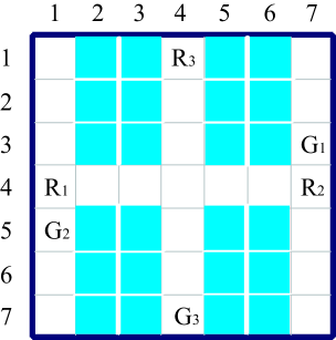
Sparse-interaction based algorithms [13] [14] have recently found wide applications in MAS research. An example of MAS with sparse interactions is the intelligent warehouse systems, where autonomous robots only consider other robots when they are close enough to each other [25] (see Fig. 1), i.e., when they meet around the crossroad. Otherwise, they can act independently.

Figure 1: A part of an intelligent warehouse with three robots, where $R_{i}$ ($i=1,2,3$) represents for robot $i$ with its corresponding goal $G_{i}$ and the shaded grids are storage shelves.

Earlier works such as the coordinated reinforcement learning [30] [31] and sparse cooperative Q-learning [32] used coordination graphs (CGs) to learn interdependencies between agents and decomposed the joint value function to local value functions. However, these algorithms cannot learn CGs online and only focus on finding specific states where coordination is necessary instead of learning for coordination [13]. Melo and Veloso [13] extended the Q-learning to a two-layer algorithm and made it possible for agents to use an additional COORDINATE action to determine the state when the coordination was necessary. Hauwere and Vrancx proposed Coordinating Q-learning (CQ-learning) [14] and FCQ-learning [33] that helped agents learn from statistical information of rewards and Q-values where an agent should take other agents’ states into account. However, all these algorithms allow agents to play greedy strategies at a certain joint state rather than equilibrium strategies, which might cause conflicts.

More recently, Hu et al [8] proposed an efficient equilibrium-based MARL method, called Negotiation-based Q-learning, by which agents can learn in a Markov game with unshared value functions and unshared joint state-actions. In later work, they applied this method for sparse interactions by knowledge transfer and game abstraction [29], and demonstrated the effectiveness of the equilibrium-based MARL in solving sparse-interaction problems. Nevertheless, as opposed to single Q-learning based approaches like CQ-learning, Hu’s equilibrium-based methods for sparse interactions require a great deal of real-time information about the joint states and joint actions of all the agents, which results in huge amount of communication costs. In this paper, we focus on solving learning problems in complex systems. Tightly coupled equilibrium-based MARL methods discussed above are impractical in these situations while sparse-interaction based algorithms tend to cause many collisions. To this end, we adopt the sparse-interaction based learning framework and each agent selects equilibrium joint actions when they are in coordination areas.

III NEGOTIATION-BASED MARL WITH SPARSE INTERACTIONS

When people work in restricted environments with possible conflicts, they usually learn how to finish their individual tasks first and then learn how to coordinate with others. We apply this commonsense to our sparse-interaction method and decompose the learning process into two distinct sub-processes [5]. First, each agent learns an optimal single-agent policy by itself in the static environment and ignores the existences of other agents. Second, each agent learns when to coordinate with others according to their immediate reward changes, and then learns how to coordinate with others in a game-theoretic way. In this section, the negotiation-based framework for MAS with sparse interactions is first introduced and then related techniques and specific algorithms are described in details.

III-A Negotiation-based Framework for Sparse Interactions

We assume that agents have learnt their optimal policies and reward models when acting individually in the environment. Two situations might occur when agents are working in a multi-agent setting. If the received immediate rewards for state-action pairs are the same as what they learned by reward models, the agents act independently. Otherwise, they need to expand their individual state-action pairs to the joint ones by adding other agents’ state-action pairs for better coordination. This negotiation-based framework for sparse interactions is given as shown in Algorithm 1, while the expansion and negotiation process is explained as follows:

0:  The agent $i$, state space $S_{i}$, action space $A_{i}$, learning rate $\alpha$, discount rate $\gamma$, exploration factor $\epsilon$ for the $\epsilon-Greedy$ exploration policy.

0:  Global Q-value $Q_{i}$ with optimal single-agent policy.

1:  for each episode do

2:     Initialize state $s_{i}$;

3:     while true do

4:        Select $a_{i}\in A_{i}$ from $Q_{i}$ with $\epsilon-Greedy$;

5:        if ($s_{i},a_{i}$) is “dangerous” then

6:           Broadcasts ($s_{i},a_{i}$) and receives ($s_{-i},a_{-i}$), form ($\vec{s},\vec{a}$);/* See Section III-D for the definitions of $s_{-i}$ and $a_{-i}$*/

7:           if ($\vec{s},\vec{a}$) is not “coordination pair” then

8:              Mark ($\vec{s},\vec{a}$) as a “coordination pair” and $\vec{s}$ as a “coordination state”, initialize Local Q-value $Q_{i}^{J}$ at $\vec{s}$ with transfer knowledge (See Equation 9);

9:           end if

10:           Negotiate for the equilibrium joint action with Algorithm 2 - Algorithm 4. Select new $\vec{a}$ with $\epsilon-Greedy$;

11:        else {detected an immediate reward change}

12:           Mark ($s_{i},a_{i}$) as “dangerous”, broadcasts ($s_{i},a_{i}$) and receives ($s_{-i},a_{-i}$), form ($\vec{s},\vec{a}$);

13:           Mark ($\vec{s},\vec{a}$) as “coordination pair” and $\vec{s}$ as “coordination state”, initialize $Q_{i}^{J}$ at $\vec{s}$ with transfer knowledge (See Equation 9);

14:           Negotiate for the equilibrium joint action with Algorithm 2 - Algorithm 4. Select new $\vec{a}$ with $\epsilon-Greedy$;

15:        end if

16:        Move to the next state $s_{i}^{\prime}$ and receive the reward $r_{i}$;

17:        if $\vec{s}$ exists then

18:           Update $Q_{i}^{J}(\vec{s},\vec{a})=(1-\alpha)Q_{i}^{J}(\vec{s},\vec{a})+\alpha(r_{i}+\gamma\max\limits_{a_{i}^{\prime}}Q_{i}(s_{i}^{\prime},a_{i}^{\prime}))$;

19:        end if

20:        Update $Q_{i}(s_{i},a_{i})=(1-\alpha)Q_{i}(s_{i},a_{i})+\alpha(r_{i}+\gamma\max\limits_{a_{i}^{\prime}}Q_{i}(s_{i}^{\prime},a_{i}^{\prime}))$;

21:        $s_{i}\leftarrow s_{i}^{\prime}$;

22:     end while until $s_{i}$ is a terminal state.

23:  end for

Algorithm 1 Negotiation-based Framework for Sparse Interactions

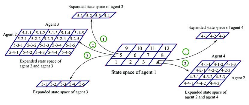
1. Broadcast joint state. Agents select an action at a certain state, and they detect a change in the immediate rewards. This state-action pair is marked as “dangerous” and these agents are called “coordinating agents”. Then, “coordinating agents” broadcast their state-action information to all other agents and receive corresponding state-action information from others. These state-action pairs with reward changes form a joint state-action and is marked as a “coordination pair”. Also, these states form a joint state called a “coordination state”, which is included in the state space of each “coordinating agent”.

2. Negotiation for equilibrium policy. When agents select a “dangerous” state-action pair, they broadcast their state-action information to each other to determine whether they are staying at a “coordination pair”. If so, the agents need to find an equilibrium policy rather than their inherent greedy policies to avoid collisions. We propose a negotiation mechanism similar to the work in [8] to find this equilibrium policy. Each “coordinating agent” broadcasts the set of strategy profiles that are potential Non-strict Equilibrium-Dominating Strategy Profile (non-strict EDSP) according to its own utilities (See Algorithm 2). If no non-strict EDSP is found, the agents search for a Meta equilibrium set (See Algorithm 3) instead, which is always nonempty [8]. Then, if there are several candidates in the equilibrium set, the agents use the minimum variance method to find the relatively good one (See Algorithm 4).

3. When an agent selects an action at a certain state, if neither a change in the immediate reward nor a “dangerous” state-action pair is detected, the agent continue to select its action independently.

Remark 1

If the number of agents $n\geq 2$, the agents may have several different expansions for different “coordination states” in one state. Each expanded joint-state is assigned an index and has a corresponding local Q-value. Once the agents form a “coordination state”, they search for the joint state in their expanded joint-state pool and obtain the corresponding local Q-value. An example is shown as in Fig. 2. In this example, agent 1-4 have twelve states, four states, five states and three states, respectively. For convenience, we assume here when agent 1 is expanding joint states, it adds all states of relevant agents in its joint states even though in most of the cases it only needs to add a small part of the states. Specifically, the fourth state of agent 1 is expanded to two joint states, the first one is with agent 4 and the second one is with agent 2 and agent 4. Similarly, the fifth state of agent 1 is expanded to three joint states, the first one is with agent 2, the second one is with agent 2 and agent 3, and the third one is with agent 3.

Remark 2

Owing to the broadcast mechanism, an agent will add the states of all the “coordinating agents” to its state space, even though it does not need to coordinate with some of these agents. The agents cannot distinguish the agent they need to coordinate with from other agents, which brings unnecessary calculations. This problem becomes more significant with the growth of the complexity of the environment and the number of the agents. Our tentative solution is setting the communication range of the agents so that they can only add neighbouring agents’ states to their state space and ignore those that do not need to coordinate with.

Remark 3

It is worth noting that if the agent detects a “dangerous” state-action pair, it should observe a reward change, that is, if we replace the former concept with the latter one, the algorithm can work equally. Defining dangerous state-action pairs mainly help us to better explain our thoughts and describe the algorithm.

Figure 2: An example of the expansion of an agent’s state space.

III-B Negotiation for Equilibrium Set

One contribution of this paper is to apply the equilibrium solution concept to traditional Q-learning based MARL algorithms. Different from previous work like CQ-learning and Learning of Coordination [14], our approach aims at finding the equilibrium solution for the one-shot game played in each “coordination state”. As a result, we focus on two pure strategy profiles [8], i.e., Non-strict Equilibrium-Dominating Strategy Profile (non-strict EDSP) and Meta Equilibrium set. The definition of Non-strict EDSP is as follows.

Definition 3

(Non-strict EDSP): In an $n$-agent ($n\geq 2$) normal-form game $\Gamma$, $\vec{e_{i}}\in A(i=1,2,\ldots,m)$ are pure strategy Nash equilibriums. A joint action $\vec{a}\in A$ is a non-strict EDSP if $\forall j\leq n$,

$$U_{j}(\vec{a})\geq\min\limits_{i}U_{j}(\vec{e_{i}})$$ (6)

The negotiation process of finding the set of Non-strict EDSP is shown as in Algorithm 2, which generally consists of two steps: 1) the agents find the set of strategy profiles that are potentially Non-strict EDSP according to their individual utilities; 2) the agents solve the intersection of all the potentially strategy sets and get the Non-strict EDSP set.

However, given the fact that the pure strategy Nash equilibrium can be non-existent in some cases, the set of Non-strict EDSP might also be empty. On this occasion, we replace this strategy profile with Meta Equilibrium, which is always nonempty. The sufficient and necessary condition of Meta Equilibrium is defined as follows.

Algorithm 2 Negotiation for Non-strict EDSPs Set

0:  A normal-form game $\langle n,\{A_{i}\}_{i=1,\ldots,n},\{U_{i}\}_{i=1,\ldots,n}\rangle$./* To be noted, “coordinating agent” $i$ only has the knowledge of $n$, $\{A_{i}\}_{i=1,\ldots,n}$ and $U_{i}$*/

0:  The set of non-strict EDSP candidates for “coordinating agents” $i$: $J_{NS}^{i}\leftarrow\emptyset$;Minimum utility value of pure strategy Nash equilibrium (PNE) candidates for “coordinating agents” $i$: $MinU_{PNE}^{i}\leftarrow\infty$;The set of non-strict EDSPs: $J_{NS}\leftarrow\emptyset$.

1:  for each $\vec{a_{-i}}\in A_{-i}$ do

2:     if $\max\limits_{a_{i}^{\prime}}U_{i}(a_{i}^{\prime},\vec{a_{-i}})<MinU_{PNE}^{i}$ then

3:        $MinU_{PNE}^{i}=\max\limits_{a_{i}^{\prime}}U_{i}(a_{i}^{\prime},\vec{a_{-i}})$;

4:     end if

5:  end for

6:  for each $\vec{a}\in A$ do

7:     if $U_{i}(\vec{a})\geq MinU_{PNE}^{i}$ then

8:        $J_{NS}^{i}\leftarrow J_{NS}^{i}\cup\{\vec{a}\}$;

9:     end if

10:  end for/* Broadcast $J_{NS}^{i}$ and corresponding utilities*/

11:  $J_{NS}\leftarrow\bigcap_{i=1}^{n}J_{NS}^{i}$

Definition 4

(Sufficient and Necessary Condition of Meta Equilibrium) [8]: In an $n$-agent ($n\geq 2$) normal-form game $\Gamma$, a joint action $\vec{a}$ is called a Meta equilibrium from a metagame $k_{1}k_{2}\ldots k_{r}\Gamma$ if and only if for any $i$ there holds

$$U_{i}(\vec{a})\geq\min\limits_{\vec{a_{P_{i}}}}\max\limits_{a_{i}}\min\limits_{\vec{a_{S_{i}}}}U_{i}(\vec{a_{P_{i}}},a_{i},\vec{a_{S_{i}}}),$$ (7)

where $P_{i}$ is the set of agents listed before sign $i$ in the prefix $k_{1}k_{2}\ldots k_{r}$, $S_{i}$ is the set of agents listed after sign $i$ in the prefix.

For example, in a three agents metagame $213\Gamma$, we have $P_{1}=\{2\},S_{1}=\{3\};P_{2}=\emptyset,S_{2}=\{1,3\};P_{3}=\{2,1\},S_{3}=\emptyset$. A Meta equilibrium $\vec{a}$ meets the following constraints:

$$\begin{split}U_{1}(\vec{a})\geq\min\limits_{a_{2}}\max\limits_{a_{1}}\min\limits_{a_{3}}U_{1}(a_{1},a_{2},a_{3}),\\ U_{2}(\vec{a})\geq\max\limits_{a_{2}}\min\limits_{a_{1}}\min\limits_{a_{3}}U_{2}(a_{1},a_{2},a_{3}),\\ U_{3}(\vec{a})\geq\min\limits_{a_{2}}\min\limits_{a_{1}}\max\limits_{a_{3}}U_{3}(a_{1},a_{2},a_{3}).\end{split}$$ (8)

Hu et al [8] used a negotiation-based method to find Meta Equilibrium set and we simplified the method as shown in Algorithm 3. It is also pointed out that both of these two strategy profiles belong to the set of symmetric meta equilibrium, which to some degree strengthens the convergence of the algorithm.

Algorithm 3 Negotiation for Meta Equilibrium Set for 3-agent games

0:  A normal-form game $<n,\{A_{i}\}_{i=1,\ldots,n},\{U_{i}\}_{i=1,\ldots,n}>$./* To be noted, “coordinating agents” $i$ only has the knowledge of $n$, $\{A_{i}\}_{i=1,\ldots,n}$ and $U_{i}$*/

0:  The set of Meta Equilibrium candidates for “coordinating agents” $i$: $J_{MetaE}^{i}\leftarrow\emptyset$;Minimum utility value of Meta Equilibrium candidates for “coordinating agents” $i$: $MinU_{MetaE}^{i}\leftarrow\infty$;The set of Meta Equilibrium: $J_{MetaE}\leftarrow\emptyset$;

1:  Randomly initialize the prefix $s_{1}s_{2}s_{3}$ from the set {123,132,213,231,312,321}.

2:  Calculate $MinU_{MetaE}^{i}$ according to Equation 7;

3:  for each $\vec{a}\in A$ do

4:     if $U_{i}(\vec{a})\geq MinU_{MetaE}^{i}$ then

5:        $J_{MetaE}^{i}\leftarrow J_{MetaE}^{i}\cup\{\vec{a}\}$;

6:     end if

7:  end for/* Broadcast $J_{MetaE}^{i}$ and corresponding utilities*/

8:  $J_{MetaE}\leftarrow\bigcap_{i=1}^{n}J_{MetaE}^{i}$

III-C Minimum Variance Method

In Section III-B, we presented the process for all “coordinating agents” to negotiate for an equilibrium joint-action set. However, the obtained set usually contains many strategy profiles and it is difficult for the agents to choose an appropriate one. In this paper a Minimum Variance method is proposed to help the “coordinating agents” choose the joint action with relatively high total utility and minimum utilities variance to guarantee the cooperation and fairness of the learning process. In addition, if the equilibrium set is nonempty, the best solution defined in the minimum variance method always exists. The minimum variance method is described in Algorithm 4.

Algorithm 4 Minimum Variance Method

0:  The equilibrium set with $m$ elements $J_{NS}=\{\vec{a_{ns}^{1}},\vec{a_{ns}^{2}},\ldots,\vec{a_{ns}^{m}}\}$ and corresponding utilities $\{U_{i}^{ns}\}_{i=1,\ldots,n}$.

0:  threshold value for total utility $\tau$;/* We set the threshold value to the mean value of the sum utilities of different joint-action profiles $\frac{\sum_{j=1}^{m}\sum_{i=1}^{n}U_{i}^{ns}(\vec{a_{ns}^{j}})}{m}$*/Minimum variance of these equilibriums $MinV\leftarrow\infty$;Best equilibrium of the non-strict EDSPs set $J_{BestNS}\leftarrow\emptyset$.

1:  for each $\vec{a_{ns}^{j}}\in J_{NS}$ do

2:     if $\sum_{i=1}^{n}U_{i}^{ns}(\vec{a_{ns}^{j}})<\tau$ then

3:        $J_{NS}\leftarrow J_{NS}\backslash\{\vec{a_{ns}^{j}}\}$;

4:     end if

5:  end for/* Minimize the joint action’s utility variance*/

6:  for each $\vec{a_{ns}^{j}}\in J_{NS}$ do

7:     if $\sqrt{\frac{1}{n}\sum_{k=1}^{n}[U_{k}^{ns}(\vec{a_{ns}^{j}})-\frac{1}{n}\sum_{i=1}^{n}U_{i}^{ns}(\vec{a_{ns}^{j}})]^{2}}<MinV$ then

8:        $MinV=\sqrt{\frac{1}{n}\sum_{k=1}^{n}[U_{k}^{ns}(\vec{a_{ns}^{j}})-\frac{1}{n}\sum_{i=1}^{n}U_{i}^{ns}(\vec{a_{ns}^{j}})]^{2}}$;

9:        $J_{BestNS}=\{\vec{a_{ns}^{j}}\}$;

10:     end if

11:  end for

12:  Output $J_{BestNS}$ as the adopted joint action.

After negotiating for one equilibrium, the agents update their states according to the joint action and receive immediate rewards, which are used to update local Q-values as well as global Q-values. Unlike other sparse-interaction algorithms (e.g., CQ-learning), we update the global optimal Q-values to avoid possible misleading information. In fact, in some cases, the selected policies in multi-agent setting are totally opposite to the agents’ individual optimal policies due to dynamic coordinating processes. The whole negotiation-based learning algorithm has already been given in Algorithm 1.

III-D Local Q-value transfer

At the beginning of the learning process, we use the transfer knowledge of agents’ optimal single agent policy to accelerate the learning process. Furthermore, it is possible to improve the algorithm performance by the local Q-value transfer. In most previous literatures [13] [14], the initial local Q-values of the newly expanded joint states are zeros. Recently, Vrancx et al proposed a transfer learning method [34] to initialize these Q-values with prior trained Q-value from the source task, which is reasonable in the real world. When people meet with others on the way to their individual destinations, they usually have prior knowledge of how to avoid collisions. Based on this prior commonsense and the knowledge of how to finish their individual tasks, the agents learn to negotiate with others and obtain fixed coordination strategies suitable for certain environments. However, Vrancx et al only used coordination knowledge to initialize the local Q-values and overlooked the environmental information, which was proved to be less effective in our experiments. In our approach, we initialize the local Q-values of newly detected “coordination” to hybrid knowledge as follows:

$$Q_{i}^{J}((s_{i},\vec{s_{-i}}),(a_{i},\vec{a_{-i}}))\leftarrow Q_{i}(s_{i},a_{i})+Q_{i}^{CT}(\vec{s},\vec{a}),$$ (9)

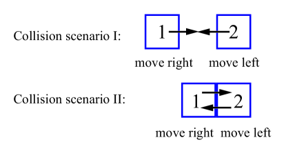
where $\vec{s_{-i}}$ is the joint-state set except for the state $s_{i}$ and $\vec{a_{-i}}$ is the joint-action set except for the action $a_{i}$, $Q_{i}^{J}((s_{i},\vec{s_{-i}}),(a_{i},\vec{a_{-i}}))$ is equal with $Q_{i}^{J}(\vec{s},\vec{a})$, $Q_{i}^{CT}(\vec{s},\vec{a})$ is the transferred Q-value from a blank source task at joint state $\vec{s}$. In this blank source task, joint action learners (JAL) [35] learn to coordinate with others disregarding the environmental information. They are given a fixed number of learning steps to learn stable Q-value $Q_{i}^{CT}(\vec{s},\vec{a})$. Similar to [34], the joint state $\vec{s}$ in $Q_{i}^{CT}(\vec{s},\vec{a})$ is presented as the relative position $(\Delta x,\Delta y)$, horizontally and vertically. When agents attempt to move into the same grid location or their previous locations (as shown in Fig. 3), these agents receive a penalty of -10. In other cases, the reward is zero.

Take a two-agent source task for example (as shown in Fig. 4(a)). The locations of agent $1$ and agent $2$ are ($4,3$) and ($3,4$), respectively. Then we have the joint state $\vec{s}=(x_{1}-x_{2},y_{1}-y_{2})=(1,-1)$ and the joint action for this joint state

$$\vec{a}=\begin{pmatrix}(a_{1},a_{2})\end{pmatrix}=\begin{pmatrix}(\uparrow,\uparrow)&(\uparrow,\downarrow)&(\uparrow,\leftarrow)&(\uparrow,\rightarrow)\\ (\downarrow,\uparrow)&(\downarrow,\downarrow)&(\downarrow,\leftarrow)&(\downarrow,\rightarrow)\\ (\leftarrow,\uparrow)&(\leftarrow,\downarrow)&(\leftarrow,\leftarrow)&(\leftarrow,\rightarrow)\\ (\rightarrow,\uparrow)&(\rightarrow,\downarrow)&(\rightarrow,\leftarrow)&(\rightarrow,\rightarrow)\end{pmatrix},$$

where $\{\uparrow,\downarrow,\leftarrow,\rightarrow\}$ denotes the action set of {up, down, left, right} for each agent. After sufficient learning steps, the agents learn their Q-value matrices at joint state $\vec{s}$ as

Figure 3: Two scenarios of possible collisions.

$$Q_{1}^{CT}(\vec{s},\bm{\cdot})=Q_{2}^{CT}(\vec{s},\bm{\cdot})=\begin{pmatrix}0&0&-10&0\\ 0&0&0&0\\ 0&0&0&0\\ 0&-10&0&0\end{pmatrix},$$

that is because when agent 1 and agent 2 select the action pair $(\uparrow,\leftarrow)$ or $(\rightarrow,\downarrow)$, a collision will occur, which leads to a -10 punishment for each agent. Otherwise, the reward is 0. Suppose that the agents are in the “coordination state” as shown in Fig. 4(b). When acting independently in the environment, the agents learn their single agent optimal Q-value vectors at state $s_{1}$ or $s_{2}$ as $Q_{1}(s_{1},\bm{\cdot})=(-1,-10,-5,-1)$, $Q_{2}(s_{2},\bm{\cdot})=(-10,-1,-1,-5)$. Then the local Q-value matrices of this “coordination state” need to be initialized as

$$\begin{aligned} Q_{1}^{J}(\vec{s},\bm{\cdot})&=Q_{1}(s_{1},\bm{\cdot})^{T}\times(1,1,1,1)+Q_{1}^{CT}(\vec{s},\bm{\cdot})\\ &=\begin{pmatrix}-1&-1&-11&-1\\ -10&-10&-10&-10\\ -5&-5&-5&-5\\ -1&-11&-1&-1\end{pmatrix},\\ Q_{2}^{J}(\vec{s},\bm{\cdot})&=(1,1,1,1)^{T}\times Q_{2}(s_{2},\bm{\cdot})+Q_{2}^{CT}(\vec{s},\bm{\cdot})\\ &=\begin{pmatrix}-10&-1&-11&-5\\ -10&-1&-1&-5\\ -10&-1&-1&-5\\ -10&-11&-1&-5\end{pmatrix}.\\ \end{aligned}$$

So the pure strategy Nash equilibria for this joint state are (up, down) and (right, left). If we initialize the local Q-value with the way used in [34] or just initialize them to zeros, the learning process would be much longer.

For the “coordination state” with three agents, the Q-value $Q_{i}^{CT}(\vec{s},\vec{a})$ can be calculated in the same way, except for the relative positions $(\Delta x_{1},\Delta y_{1},\Delta x_{2},\Delta y_{2})=(x_{1}-x_{2},y_{1}-y_{2},x_{2}-x_{3},y_{2}-y_{3})$ and the cubic Q-value for each joint state.

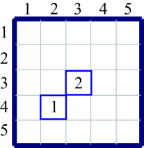
(a) A $5\times 5$ blank source task with two agents.

(b) The detected “coordination states”.

Figure 4: An example of the local Q-value transfer in a two-agent system.

IV EXPERIMENTS

To test the presented NegoSI algorithm, several groups of simulated experiments are implemented and the results are compared with those of three other state-of-the-art MARL algorithms, namely, CQ-learning [14], NegoQ with value function transfer (NegoQ-VFT) [29] and independent learners with value function transfer (IL-VFT). In next two subsections, the presented NegoSI algorithm is applied to six grid world games and an intelligent warehouse problem, which shows that NegoSI is an effective approach for MARL problems compared with other existing MARL algorithms.

For all these experiments, each agent has four actions: up, down, left, right. The reward settings are as follows:

1. When an agent reaches its goal/goals, it receives a reward of 100. Its final goal is an absorbing state. One episode is over when all agents reach their goals.

2. A negative reward of -10 is received if a collision happens or an agent steps out of the border. In these cases, agents will bounce to their previous states.

3. Otherwise, the reward is set to -1 as the power consumption.

The settings of other parameters are the same for all algorithms: learning rate $\alpha=0.1$, discount rate $\gamma=0.9$, exploration factor $\epsilon=0.01$ for $\epsilon$-greedy strategy. All algorithms run $2000$ iterations for the grid world games and $8000$ iterations for the intelligent warehouse problem. We use three typical criteria to evaluate these MARL algorithms, i.e., steps of each episode (SEE), rewards of each episode (REE) and average runtime (AR). All the results are averaged over 50 runs.

IV-A Tests on grid world games

(a) ISR

(b) SUNY

(c) MIT

(d) PENTAGON

(e) GW_nju

(f) GWa3

Figure 5: Grid world games.

TABLE I: The learning steps of the final episode of each tested benchmark map.

	$ISR$	$SUNY$	$MIT$	$PENTAGON$	$GW\_{nju}$	$GWa3$
$CQ-learning$	$8.91$	$10.70$	$19.81$	$15.32$	$12.65$	$8.65$
$ILVFT$	$13.11$	10.38	18.67	$14.18$	10.94	$11.40$
$NegoQVFT$	$8.36$	$12.98$	$19.81$	8.55	$10.95$	8.31
$NegoSI$	7.48	$10.92$	$21.29$	$10.30$	$12.11$	$8.87$
$The\ optimal\ policy$	$6$	$10$	$18$	$8$	$10$	$8$

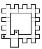
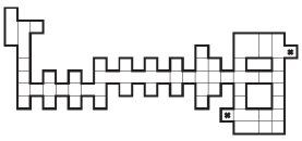
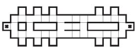
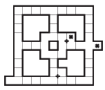
The proposed NegoSI algorithm is evaluated in the grid world games presented by Melo and Veloso [13], which are shown in Fig. 5. The first four benchmarks, i.e., ISR, SUNY, MIT and PENTAGON (shown as Fig. 5(a)-(d), respectively), are two-agent games, where the cross symbols denote the initial locations of each agent and the goals of the other agent. In addition, we design two highly competitive games to further test the algorithms, namely, GW_nju (Fig. 5(e)) and GWa3 (Fig. 5(f)). The game GW_nju has two agents and the game GWa3 has three agents. The initial location and the goal of agent $i$ are represented by the number $i$ and $G_{i}$, respectively.

(a) ISR

(b) SUNY

(c) MIT

(d) PENTAGON

(e) GW_nju

(f) GWa3

Figure 6: SEE (steps of each episode) for each tested benchmark map.

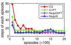
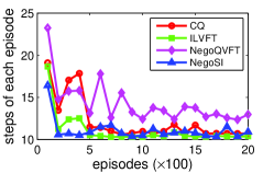
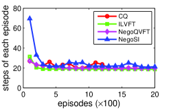
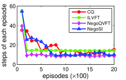
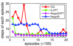
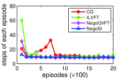
We first examine the performances of the tested algorithms regarding the SEE (steps of each episode) for each benchmark map (See Fig. 6). The state-of-the-art value function transfer mechanism helps NegoQ and ILs to converge fast in all games except for SUNY. NegoSI also has good convergence characteristics. CQ-learning, however, has a less stable learning curve especially in PENTAGON, GW_nju and GWa3. This is reasonable since in these highly competitive games, the agents’ prior-learned optimal policies always have conflicts and CQ-learning cannot find the equilibrium joint action to coordinate them. When more collisions occur, the agents are frequently bounced to previous states and forced to take more steps before reaching their goals. The learning steps of the final episode for each algorithm in each benchmark map are shown in Table I. In ISR, NegoSI converges to 7.48, which is the closest one to the value obtained by the optimal policy. In other cases, NegoSI achieves the learning step of the final episode between 105.1% and 120.4% to the best solution.

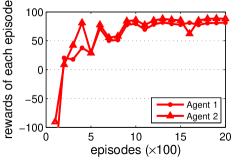
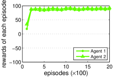
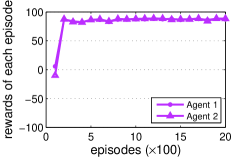
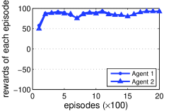
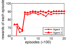
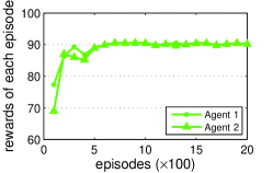
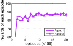
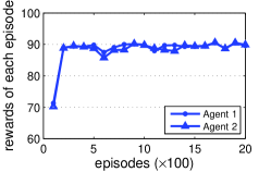
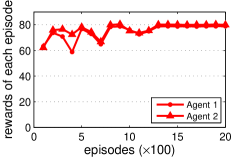
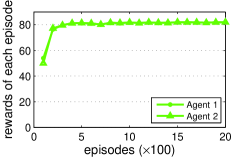
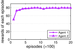
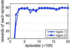
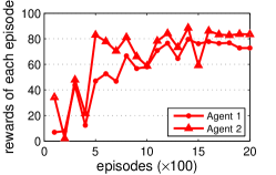
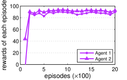
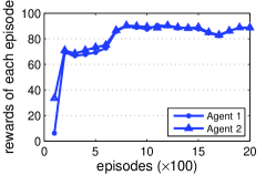
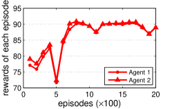
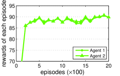
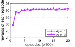
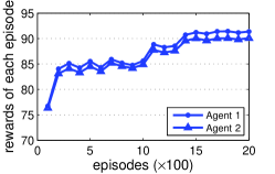
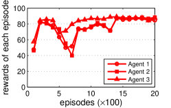
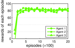
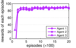
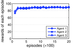
Then we analyze the REE (rewards of each episode) criterion of these tested algorithms (See Fig. 7-12). The results vary for each map. In ISR, NegoSI generally achieves the highest REE through the whole learning process, which shows fewer collisions and more cooperations between the learning agents. Also, the difference between the two agents’ reward values is small, which reflects the fairness of the learning process of NegoSI. The agents are more independent in SUNY. Each of them has three candidates for the single-agent optimal policy. In this setting, ILVFT has good performance. NegoSI shows its fairness and high REE value compared with NegoVFT and CQ-learning. The agents in MIT have more choices of collision avoidances. All the tested algorithms obtain the final reward of around 80. However, the learning curves of CQ-learning are relatively unstable. In PENTAGON, NegoSI proves its fairness and achieves as good performance as algorithms do with the value function transfer.

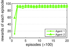
Other than these above benchmarks, we give two highly competitive games to test the proposed algorithm. In both games, the agents’ single-agent optimal policies conflict with each other and need appropriate coordination. In GW_nju, the learning curves of NegoSI finally converge to 91.39 and 90.09, which are very close to the optimal final REE values as 93 and 91, respectively. Similar to NegoSI, NegoVFT achieves the final REE values of 91.27 and 91.25. However, NegoSI can negotiate for a fixed and safer policy that allows one agent to always move greedily and the other to avoid collision (while NegoVFT cannot), which shows the better coordination ability of NegoSI. For the three-agent grid world GWa3, even though NegoSI does not have the lowest SEE, it achieves the highest REE through the whole learning process. For one thing, this result demonstrates the scalability of NegoSI in the three-agent setting. For another, it shows that the agents using NegoSI have the ability to avoid collisions to obtain more rewards while the agents using traditional MARL methods have less desire to coordinate and therefore lose their rewards. Actually, even though we developed our method with non-cooperative multi-agent model, it does not necessarily mean that the agents are egoistic. Thanks to the negotiation mechanism, agents learn to benefit themselves while doing little harm to others, which shows an evidence of cooperation.

(a) CQ-learning

(b) ILVFT

(c) NegoQVFT

(d) NegoSI

Figure 7: REE (rewards of each episode) for each tested algorithm in ISR.

(a) CQ-learning

(b) ILVFT

(c) NegoQVFT

(d) NegoSI

Figure 8: REE (rewards of each episode) for each tested algorithm in SUNY.

(a) CQ-learning

(b) ILVFT

(c) NegoQVFT

(d) NegoSI

Figure 9: REE (rewards of each episode) for each tested algorithm in MIT.

(a) CQ-learning

(b) ILVFT

(c) NegoQVFT

(d) NegoSI

Figure 10: REE (rewards of each episode) for each tested algorithm in PENTAGON.

(a) CQ-learning

(b) ILVFT

(c) NegoQVFT

(d) NegoSI

Figure 11: REE (rewards of each episode) for each tested algorithm in GW_nju.

(a) CQ-learning

(b) ILVFT

(c) NegoQVFT

(d) NegoSI

Figure 12: REE (rewards of each episode) for each tested algorithm in GWa3.

TABLE II: Average runtime for each tested map.

	$ISR$	$SUNY$	$MIT$	$PENTAGON$	$GW\_{nju}$	$GWa3$
$CQ-learning$	$8.54$	$5.91$	$13.68$	$8.52$	$5.07$	$5.95$
$ILVFT$	$4.91$	$4.14$	$9.78$	$6.56$	$2.53$	$7.21$
$NegoQVFT$	$13.92$	$20.18$	$36.84$	$18.45$	$21.89$	$50.48$
$NegoSI$	$16.74$	$7.33$	$19.58$	$16.18$	$7.08$	$16.41$
$QL\ for\ Single\ Policy$	$0.51$	$0.45$	$1.29$	$0.05$	$0.19$	$0.07$

The results regarding AR (average runtime) are shown in Table II. ILVFT has the fastest learning speed, which is only five to ten times slower than Q-learning to learn single policy. CQ-learning only considers joint states in “coordination state” and it also has a relatively small computational complexity. The AR of NegoVFT is five to ten times more than that of ILVFT. This is reasonable since NegoVFT learns in the whole joint state-action space and computes the equilibrium for each joint state. The learning speed of NegoSI is slower than CQ-learning but faster than NegoVFT. Even if NegoSI adopts the sparse-interaction based learning framework and has computational complexity similar to CQ-learning, it needs to search for the equilibrium joint action in the “coordination state”, which slows down the learning process.

IV-B A real-world application: intelligent warehouse systems

Figure 13: Simulation platform of the intelligent warehouse system.

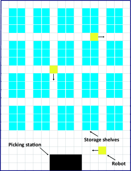
MARL has been widely used in such simulated domains as grid worlds [1], but few applications have been found for realistic problems comparing to single-agent RL algorithms [36]-[39] or MAS algorithms [40]-[42]. In this paper, we apply the proposed NegoSI algorithm to an intelligent warehouse problem. Previously, single agent path planning methods have been successfully used in complex systems [43] [44], however, the intelligent warehouse employs a team of mobile robots to transport objects and single-agent path planning methods frequently cause collisions [45]. So we solve the multi-agent coordination problem in a learning way.

The intelligent warehouse is made up of three parts: picking stations, robots and storage shelves (shown as in Fig. 13). There are generally four steps of the order fulfillment process for intelligent warehouse systems:

1. Input and decomposition: input and decompose orders into separated tasks;

2. Task allocation: the central controller allocates the tasks to corresponding robots using task allocation algorithms (e.g., the Auction method);

3. Path planning: robots plan their transportation paths with a single-agent path planning algorithm;

4. Transportation and collision avoidance: robots transport their target storage shelves to the picking station and then bring them back to their initial positions. During the transportation process, robots use sensors to detect shelves and other robots to avoid collisions.

We focus on solving the multi-robot path planning and collision avoidance in a MARL way and ignore the first two steps of the order fulfillment process by requiring each robot to finish a certain number of random tasks. The simulation platform of an intelligent warehouse system is shown as in Fig. 13, which is a $16\times 21$ grid environment and each grid is of size $0.5m\times 0.5m$ in real world. Shaded grids are storage shelves which cannot be passed through. The state space of each robot is made up of two parts: the location and the task number. Each robot has 4 actions, namely, “up”, “down”, “left” and “right”.

(a) SEE

(b) REE

Figure 14: SEE (steps of each episode) and REE (rewards of each episode) for NegoSI and CQ-learning in the 2-agent intelligent warehouse.

(a) SEE

(b) REE

Figure 15: SEE (steps of each episode) and REE (rewards of each episode) for NegoSI and CQ-learning in the 3-agent intelligent warehouse.

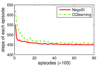
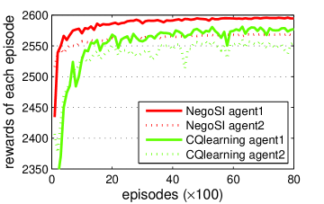
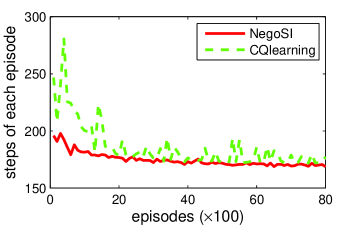
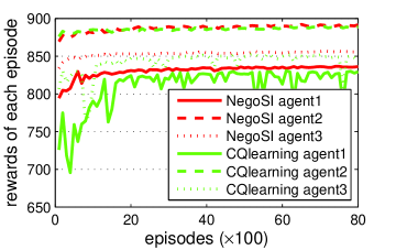
We only compare the NegoSI algorithm with CQ-learning for the intelligent warehouse problem. In fact, ILVFT has no guarantee of the convergence characteristics and it is difficult to converge in the intelligent warehouse setting in practice. NegoVFT is also infeasible since its internal memory cost in MATLAB is estimated to be $208\times 208\times 208\times 10\times 10\times 10\times 4\times 4\times 4\times 8B=4291GB$, while the costs of other algorithms are about 2 MB. Like NegoVFT, other MG-based MARL algorithms cannot solve the intelligent warehouse problem either. Experiments were performed in 2-agent and 3-agent settings, respectively, and the results are shown as in Fig. 14 and Fig. 15.

In the 2-agent setting, the initial position and final goal of robot $1$ are ($1,1$) and those of robot $2$ are ($1,16$). Each robot needs to finish 30 randomly assigned tasks. The task set is the same for all algorithms. Robots with NegoSI achieve lower SEE (steps of each episode) than robots with CQ-learning throughout the whole learning process (as shown in Fig. 14). NegoSI finally converges to 449.9 steps and CQ-learning converges to 456.9 steps. In addition, robots with NegoSI have higher and more stable REE (rewards of each episode). Finally, the average runtime for completing all the tasks is $2227$s for NegoSI and is $3606$s for CQ-learning. Robots used 38% less time to complete all the tasks with NegoSI than that with CQ-learning.

The performances of NegoSI are also better in the 3-agent setting than that of CQ-learning. The initial position and the final goal of different robots are ($1,1$), ($1,8$) and ($1,16$). Each robot needs to finish $10$ randomly assigned tasks. The task set is the same for different algorithms. SEE (steps of each episode) for robots with NegoSI finally converges to $168.7$ steps and that for robots with CQ-learning converges to $177.3$ steps (as shown in Fig. 15). In addition, the learning curves of NegoSI are more stable. Robots with NegoSI have higher and more stable REE (rewards of each episode). Finally, the average runtime for completing all the tasks is $1352$s for NegoSI and $2814$s for CQ-learning. The robots use 52% less time to complete all the tasks with NegoSI than that with CQ-learning.

Remark 4

The agents with CQ-learning algorithm learn faster than the agents with NegoSI for the benchmark maps in Section IV-A, but slower than those with NegoSI for the intelligent warehouse problem in Section IV-B. The reason is that for agents with CQ-learning, the number of “coordination state” is several times higher than that with NegoSI. This difference becomes significant with the increase of the task number, the environment scale and the number of agents. Thus, the time used to search for one specific “coordination state” in the “coordination state” pool increases faster in CQ-learning than in NegoSI, which results in the increase of the whole learning time. According to all these experimental results, the presented NegoSI algorithm maintains better performances regarding such characteristics as coordination ability, convergence, scalability and computational complexity, especially for practical problems.

V Conclusions

In this paper a negotiation-based MARL algorithm with sparse interactions (NegoSI) is proposed for the learning and coordination problems in multi-agent systems. In this integrated algorithm the knowledge transfer mechanism is also adopted to improve agent’s learning speed and coordination ability. In contrast to traditional sparse-interaction based MARL algorithms, NegoSI adopts the equilibrium concept and makes it possible for agents to select non-strict EDSP or Meta equilibrium for their joint actions, which makes it easy to find near optimal (or even optimal) policy and to avoid collisions as well. The experimental results demonstrate the effectiveness of the presented NegoSI algorithm regarding such characteristics as fast convergence, low computational complexity and high scalability in comparison to the state-of-the-art MARL algorithms, especially for practical problems. Our future work focuses on further comparison of NegoSI with other existing MARL algorithms and more applications of MARL algorithms to general and realistic problems. In addition, multi-objective reinforcement learning (MORL) [46]-[48] will also be considered to further combine environment information and coordination knowledge for local learning.

References

- [1] L. Buşoniu, R. Babuška and B. D. Schutter, “A comprehensive survey of multi-agent reinforcement learning,” IEEE Transactions on System, Man, and Cybernetics, Part C: Applications and Reviews, vol. 38, no. 2, pp. 156-172, 2008.
- [2] P. Vrancx, K. Verbeeck and A. Nowé, “Decentralized learning in markov games,” IEEE Transactions on Systems, Man, and Cybernetics, Part B: Cybernetics, vol. 38, no. 4, pp. 976-981, 2008.
- [3] R. Bianchi, M. F. Martins, C. H. Ribeiro and A. H. Costa, “Heuristically-accelerated multiagent reinforcement learning,” IEEE Transactions on Cybernetics, vol. 44, no. 2, pp. 252-265, 2014.
- [4] K. Hwang, S. Tan, M. Hsiao and C. Wu, “Cooperative multiagent congestion control for high-speed networks,” IEEE Transactions on Systems, Man, and Cybernetics, Part B: Cybernetics, vol. 35, no. 2, pp. 255-268, 2005.
- [5] C. Yu, M. Zhang, F. Ren and G. Tan, “Multiagent learning of coordination in loosely coupled multiagent systems,” IEEE Transaction on Cybernetics, vol. 45, no. 12, pp. 2853-2867, 2015.
- [6] M. L. Littman, “Markov games as a framework for multi-agent reinforcement learning,” in Proceedings of the International Conference on Machine Learning (ICML-94), pp.157-163, New Brunswick, NJ, July 10-13, 1994.
- [7] F. S. Melo and M. Veloso, “Decentralized MDPs with sparse interactions,” Artificial Intelligence, vol. 175, no. 11, pp. 1757-1789, 2011.
- [8] Y. Hu, Y. Gao and B. An, “Multiagent reinforcement learning with unshared value functions,” IEEE Transaction on Cybernetics, vol. 45, no. 4, pp. 647-662, 2015.
- [9] Y. Hu, Y. Gao and B. An, “Accelerating multiagent reinforcement learning by equilibrium transfer,” IEEE Transaction on Cybernetics, vol.45, no. 7, pp. 1289 - 1302, 2015.
- [10] J. Hu and M. P. Wellman, “Nash Q-learning for general-sum stochastic games,” The Journal of Machine Learning Research, vol. 4, pp. 1039 C1069, 2003.
- [11] M. L. Littman, “Friend-or-foe Q-learning in general-sum games,” in Proceedings of the International Conference on Machine Learning (ICML-01), pp. 322-328, Williams College, Williamstown, MA, USA, 2001.
- [12] A. Greenwald, K. Hall and R. Serrano, “Correlated Q-learning,” in Proceedings of the International Conference on Machine Learning (ICML-03), pp. 84-89, Washington, DC, USA, 2003.
- [13] F. S. Melo and M. Veloso, “Learning of coordination: Exploiting sparse interactions in multiagent systems,” in Proceedings of the International Conference on Autonomous Agents and Multiagent Systems (AAMAS), pp. 773-780, 2009.
- [14] Y. D. Hauwere, P. Vrancx and A. Nowé, “Learning multi-agent state space representations,” in Proceedings of the International Conference on Autonomous Agents and Multiagent Systems (AAMAS), vol. 1, no. 1, pp. 715-722, 2010.
- [15] Y. D. Hauwere, P. Vrancx and A. Nowé, “Generalized learning automata for multi-agent reinforcement learning,” AI Communications, vol. 23, no. 4, pp. 311-324, 2010.
- [16] W. Wang and Y. Jiang, “Community-aware task allocation for social networked multiagent systems,” IEEE Transactions on Cybernetics, vol. 44, no. 9, pp. 1529-1543, 2014.
- [17] J. Enright and P. R. Wurman, “Optimization and coordinated autonomy in mobile fulfillment systems,” Automated Action Planning for Autonomous Mobile Robots, pp. 33-38, 2011.
- [18] P. Stone and M. Veloso, “Multiagent systems: a survey from the machine learning perspective,” Autonomous Robots, vol. 8, no. 3, pp. 345-383, 2000.
- [19] J. F. Nash, “Equilibrium points in n-person games,” in Proceedings of the National Academy of Sciences of the United States of America, vol. 36, no. 1, pp. 48-49, 1950.
- [20] B. An, F. Douglis and F. Ye, “Heuristics for negotiation schedules in multi-plan optimization,” in Proceedings of the International Conference on Autonomous Agents and Multiagent Aystems (AAMAS), vol. 2, pp. 551-558, 2008.
- [21] B. An, V. Lesser, D. Westbrook and M. Zink, “Agent-mediated multi-step optimization for resource allocation in distributed sensor networks,” in Proceedings of the International Conference on Autonomous Agents and Multiagent Systems (AAMAS), vol. 2, pp. 609-616, 2011.
- [22] R. S. Sutton and A. G. Barto, “Reinforcement learning: an introduction,” MIT press, 1998.
- [23] C. Watkins, “Learning from delayed rewards,” PhD thesis, University of Cambridge, 1989.
- [24] J. Tsitsiklis, “Asynchronous stochastic approximation and Q-learning,” Machine Learning, vol. 16, no. 3, pp. 185-202, 1994.
- [25] A. Nowé, P. Vrancx, and Y. D. Hauwere, “Game theory and multi-agent reinforcement learning,” Reinforcement Learning, Springer Berlin Heidelberg, pp. 441-470, 2012.
- [26] A. Burkov and B. Chaib-Draa, “Repeated games for multiagent systems: a survey,” The Knowledge Engineering Review, vol. 29, no. 1, pp. 1-30, 2014.
- [27] A. Burkov and B. Chaib-Draa, “An approximate subgame-perfect equilibrium computation technique for repeated games,” Proceedings of the Twenty-Fourth AAAI Conference on Artificial Intelligence, pp. 729-736, 2010.
- [28] R. Porter, E. Nudelman and Y. Shoham, “Simple search methods for finding a Nash equilibirum,” Games and Economic Behavior, vol. 63, no. 2, pp. 642-662, 2008.
- [29] Y. Hu, Y. Gao and B. An, “Learning in Multi-agent Systems with Sparse Interactions by Knowledge Transfer and Game Abstraction,” in Proceedings of the International Conference on Autonomous Agents and Multiagent Systems (AAMAS), pp. 753-761, Istanbul, Turkey, 4-8 May, 2015.
- [30] C. Guestrin, M. Lagoudakis and R. Parr, “Coordinated reinforcement learning,” in Proceedings of the International Conference on Machine Learning (ICML-02), vol. 2, pp. 227-234. 2002.
- [31] C. Guestrin, S. Venkataraman and D. Koller, “Context-specific multiagent coordination and planning with factored MDPs,” in Proceedings of the National Conference on Artificial Intelligence, pp. 253-259. 2002.
- [32] J. R. Kok and N. A. Vlassis, “Sparse cooperative Q-learning,” in Proceedings of the International Conference on Machine Learning (ICML-04), pp. 61-68, Banff, Alberta, Canada, 2004.
- [33] Y. D. Hauwere, P. Vrancx, and A. Nowé, “Solving sparse delayed coordination problems in multi-agent reinforcement learning,” Adaptive and Learning Agents, Springer Berlin Heidelberg, pp. 114-133, 2012.
- [34] P. Vrancx, Y. D. Hauwere and A. Nowé, “Transfer learning for multi-agent coordination,” in Proceedings of the International Conference on Agents and Artificial Intelligence (ICAART), pp. 263-272, 2011.
- [35] C. Claus and C. Boutilier, “The dynamics of reinforcement learning in cooperative multiagent systems,” in Proceedings of the fifteenth national/tenth conference on Artificial intelligence/Innovative applications of artificial intelligence, pp. 746-752, July 26 C30, 1998.
- [36] D. Liu, X. Yang, D. Wang and Q. Wei, “Reinforcement-learning-based robust controller design for continuous-time uncertain nonlinear systems subject to input constraints,” IEEE Transactions on Cybernetics, vol. 45, no. 7, pp. 1372-1385, 2015.
- [37] S. Haeri and L. Trajkovic, “Intelligent Deflection Routing in Buffer-Less Networks,” IEEE Transactions on Cybernetics, vol. 45, no. 2, pp. 316-327, 2015.
- [38] D. Ernst, M. Glavic, F. Capitanescu and L. Wehenkel, “Reinforcement learning versus model predictive control: a comparison on a power system problem,” IEEE Transactions on Systems, Man, and Cybernetics, Part B: Cybernetics, vol. 39, no. 2, pp. 517-529, 2009.
- [39] J. Valasek, J. Doebbler, M. D. Tandale and A. J. Meade, “Improved adaptive-reinforcement learning control for morphing unmanned air vehicles,” IEEE Transactions on Systems, Man, and Cybernetics, Part B: Cybernetics, vol. 38, no. 4, pp. 1014-1020, 2008.
- [40] L. Sabattini, C. Secchi and N. Chopra, “Decentralized estimation and control for preserving the strong connectivity of directed graphs,” IEEE Transactions on Cybernetics, vol. 45, no. 10, pp. 2273-2286, 2015.
- [41] S. Su, Z. Lin and A. Garcia, “Distributed synchronization control of multiagent systems with unknown nonlinearities,” IEEE Transactions on Cybernetics, vol. 46, no. 1, pp. 325-338, 2016.
- [42] H. Zhang, T. Feng, G. Yang and H. Liang, “Distributed cooperative optimal control for multiagent systems on directed graphs: an inverse optimal approach,” IEEE Transactions on Cybernetics, vol. 45, no. 7, pp. 1315-1326, 2015.
- [43] L. Zhou, Y. Shi, J. Wang and P. Yang, “A balanced heuristic mechanism for multirobot task allocation of intelligent warehouses,” Mathematical Problems in Engineering, vol. 2014, article ID 380480, 2014.
- [44] H. H. Viet, P. H. Kyaw and T. Chung. “Simulation-based evaluations of reinforcement learning algorithms for autonomous mobile robot path planning,” IT Convergence and Services, Springer Netherlands, pp. 467-476, 2011.
- [45] P. R. Wurman, R. D’Andrea and M. Mountz, “Coordinating hundreds of cooperative, autonomous vehicles in warehouses,” AI Magazine, vol. 29, no. 1, pp. 9-20, 2008.
- [46] P. Vamplew, R. Dazeley, A. Berry, R. Issabekov and E. Dekker, “Empirical evaluation methods for multiobjective reinforcement learning algorithms,” Machine Learning, vol. 84, no. 1-2, pp. 51-80, 2011.
- [47] C. Lin and I. Chung, “A reinforcement neuro-fuzzy combiner for multiobjective control,” IEEE Transactions on Systems, Man, and Cybernetics, Part B: Cybernetics, vol. 29, no. 6, pp. 726-744, 1999.
- [48] C. Liu, X. Xu and D. Hu, “Multiobjective reinforcement learning: A comprehensive overview,” IEEE Transactions on Systems, Man, and Cybernetics: Systems, vol. 45, no. 3, pp. 385-398, 2015.