Asymptotic Efficiency of Goodness-of-fit Tests Based on Too-Lin Characterization

Abstract

In this paper a new class of uniformity tests is proposed. It is shown that those tests are applicable to the cases of any simple null hypothesis as well as for the composite null hypothesis of rectangular distributions on arbitrary support. The asymptotic properties of test statistics are examined. The tests are compared with some standard and some recent uniformity tests. For each test the Bahadur efficiencies against some common local alternatives are calculated. A class of locally optimal alternatives is found for each proposed test. The power study is also provided. Some applications in time series analysis are presented.

keywords: testing uniformity, moments of order statistics,
Bahadur efficiency, $U$-statistics, conditional duration models.

MSC(2010): 60F10, 62G10,  62G20, 62G30

1 Introduction

The uniform distribution is one of the most used distribution in statistical modeling and computer science. Therefore ensuring that the data come from uniform distribution is of huge importance. Moreover, testing that the data come from a particular distribution can be easily reduced to testing uniformity. More about such goodness-of-fit techniques can be found in [5] and [7].

In recent times, the tests based on some characteristic property that distribution possesses have become very popular. Many different types of characterizations can be found e.g in [10]. Some characterizations of the uniform distribution can be found e.g in [1], [11], [34]. The first uniformity test based on a characterization that involves moments, was proposed in [13]. Their test was based on Papathanasiou’s characterization on maximal covariance between the minimum and the maximum of a sample of the size two, presented in [31]. Other tests based on characterizations via moments have been considered in, among others, [23], [24].

One way to compare tests is to calculate their asymptotic efficiencies. In the case of non-normal limiting distribution, the Bahadur approach to efficiency is suitable (see [2] and [25]). Among recent papers, it has been considered in e.g. [32], [28], [12], [15], [29], [30], [20], [21], [22].

In this paper we propose new uniformity tests based on the characterization from [33], that involves some moments of order statistics. We examine the asymptotic properties of the test statistics. This characterization has already been used in [23], however the nature of their test is completely different.

The paper is organized as follows. In Section 2 we present the characterization and a class of test statistics based on it. Next, we give a brief introduction to Bahadur theory. Using the Bahadur efficiency we compare our test with Hashimoto-Shirahata test based on a maximal covariance characterization (see [13]), Fortiana-Grané test based on maximum correlations (see [12]), as well as some standard goodness-of-fit tests. Additionally, for each proposed test we find some classes of locally optimal alternatives. Next we compare the Bahadur efficiencies of presented tests in the case of testing the null hypothesis of standard normal, standard logistic and standard Cauchy distribution against location alternatives. Finally, we adapt our tests for testing ”rectangularity” on an unknown support. In Section 4 we perform a power study and present some applications in time series analysis.

2 Characterization and Test Statistics

In [33] the following characterization of the uniform distribution is proved.

Theorem 2.1

Let the kth order statistic from the i.i.d. sample of size $m$, $X_{(k),m}$ has finite second moment, $EX_{(k),m}^{2}<\infty$ for some pair $(k,m)$. Then the equality

$$EX^{2}_{(k),m}-\frac{2k}{m+1}EX_{(k+1),m+1}+\frac{k(k+1)}{(m+1)(m+2)}=0$$ (1)

holds if and only if $F(x)=x$ on $(0,1)$.

Denote $X_{(a),X_{1},...,X_{n}}$ the $a$th order statistic of the i.i.d. sample $X_{1},...,X_{n}$. We test the null hypothesis $H_{0}:(F(x)=x,\;x\in(0,1))$. In view of the characterization for $k=1$, we propose the following class of test statistics.

$$T^{(m)}_{n} =\frac{1}{\binom{n}{m+1}}\sum\limits_{i_{1}<\cdots<i_{m+1}}\Big{(}\frac{1}{(m+1)!}\sum\limits_{\pi\in\Pi(m+1)}\!\!\!X_{(1),X_{i_{\pi(1)}},...,X_{i_{\pi(m)}}}^{2}$$

$$-\frac{2}{m+1}X_{(2),X_{i_{1}},...,X_{i_{m+1}}}+\frac{2}{(m+1)(m+2)}\Big{)},$$

where $\Pi(m)$ is the set of all one-to-one mappings $\pi:\{1,....,m\}\mapsto\{1,....,m\}.$

We consider large absolute values of test statistic to be significant.

Notice that these statistics are $U$-statistics with symmetric kernels

$$\Phi_{m}(X_{1},..,X_{m+1}) =\frac{1}{(m+1)!}\sum\limits_{\pi\in\Pi(m+1)}\!\!\!X_{(1),X_{\pi(1)},...,X_{\pi(m)}}^{2}-\frac{2}{m+1}X_{(2),X_{1},...,X_{{m+1}}}$$

$$+\frac{2}{(m+1)(m+2)},$$

where $\Pi(m)$ is the set of all permutations of numbers $1,2,...,m$.

The first projections of the kernels $\Phi_{m}(X_{1},..,X_{m+1})$ on $X_{m+1}$ under $H_{0}$ are

$$\phi_{m}(s) =E(\Phi_{m}(X_{1},..,X_{m+1})|X_{m+1}=s)=\frac{m}{m+1}E(X^{2}_{(1),s,X_{1},...,X_{m-1}})$$

$$+\frac{1}{m+1}E(X^{2}_{(1),X_{1},...,X_{m}})-\frac{2}{m+1}E(X_{(2),s,X_{1},...,X_{m}})+\frac{2}{(m+1)(m+2)}.$$

We have

$$E(X^{2}_{(1),s,X_{1},...,X_{m-1}}) =E(X^{2}_{(1),X_{1},...,X_{m-1}}I\{X_{(1),X_{1},...,X_{m-1}}<s\})$$

$$+s^{2}P\{X_{(1),X_{1},...,X_{m-1}}>s\}$$

$$=\frac{2-2(1-s)^{m}(ms+1)}{m(m+1)}.$$

Similarly,

$$E(X^{2}_{(1),X_{1},...,X_{m}}) =\int_{0}^{1}y^{2}\cdot m(1-y)^{m-1}dy=\frac{2}{(m+1)(m+2)},$$

$$E(X_{(2),s,X_{1},...,X_{m}}) =E(X_{(1),X_{1},...,X_{m}}I\{s<X_{(1),X_{1},...,X_{m}}\})$$

$$+sP\{X_{(1),X_{1},...,X_{m}}<s<X_{(2),X_{1},...,X_{m}}\}$$

$$+E(X_{(2),X_{1},...,X_{m}}I\{s>X_{(2),X_{1},...,X_{m}}\})$$

$$=\int_{s}^{1}y\cdot m(1-y)^{m-1}dy$$

$$+s\cdot ms(1-s)^{m-1}$$

$$+\int_{0}^{s}y\cdot m(m-1)y(1-y)^{m-2}dy$$

$$=\frac{2-(1-s)^{m}(ms+1)}{m+1}.$$

Therefore, the first projections are equal to zero under the null hypothesis. Hence, the statistics $T^{(m)}_{n}$ are degenerate for every $m$.

The second projections of $\Phi_{m}(X_{1},..,X_{m+1})$ on $(X_{m},X_{m+1})$ under the null hypothesis are

$$\phi^{\ast}_{m}(s,t) =E(\Phi_{m}(X_{1},..,X_{m+1})|X_{m}=s,X_{m+1}=t)$$

$$=\frac{m-1}{m+1}E(X^{2}_{(1),s,t,X_{1},...,X_{m-2}})+\frac{1}{m+1}E(X^{2}_{(1),s,X_{1},...,X_{m-1}})$$

$$+\frac{1}{m+1}E(X^{2}_{(1),t,X_{1},...,X_{m-1}})-\frac{2}{m+1}E(X_{(2),s,t,X_{1},...,X_{m-1}})$$

$$+\frac{2}{(m+1)(m+2)}.$$

Using the same reasoning as before, after some calculations, we obtain

$$\phi^{\ast}_{m}(s,t) =-\frac{2}{m(1+m)^{2}(2+m)}\Big{(}-2+2(1-t)^{m}+m^{2}\big{(}-(1-s)^{m+1}$$

$$+(1-t)^{m}t\big{)}+m\big{(}-2(1-s)^{m+1}+(1-t)^{m}+2(1-t)^{m}t\big{)}\Big{)}$$

$$+\frac{2}{m(1+m)}I\{s<t\}((1-t)^{m}-(1-s)^{m}).$$

Obviously, $\phi^{\ast}_{m}$ is not equal to zero for any choice of $m$. Therefore we conclude that the kernels of our test statistics are weakly degenerate.

Using Theorem 4.4.1 from [17] for weakly degenerate $U$-statistics we have

$$nT^{(m)}_{n}\overset{d}{\rightarrow}\binom{m+1}{2}\sum\limits_{i=1}^{\infty}\nu^{(m)}_{i}(\tau^{2}_{i}-1),$$

where ${\nu^{(m)}_{i}}$ are the eigenvalues of the integral operator $S$ defined by

$$Sf(t)=\int\limits_{0}^{1}\phi^{\ast}_{m}(s,t)f(s)ds.$$ (2)

Thus we have to solve the following integral equation

$$\nu^{(m)}f(t)=\int\limits_{0}^{1}\phi^{\ast}_{m}(s,t)f(s)ds,$$ (3)

with constraint $\int\limits_{0}^{1}f(s)ds=0$.

Denote $y(t)=\int_{0}^{t}f(s)ds$. After the differentiation, the expression (3) becomes

$$\nu^{(m)}y^{\prime\prime}(t)=-2\frac{(1-t)^{m-1}}{m+1}y(t),\;\;\;y(0)=0,\;\;y(1)=0.$$

After the change of variables $s=1-t$, $\lambda^{(m)}=\frac{1}{\nu^{(m)}},$ we obtain the following boundary problem

$$y^{\prime\prime}(s)+\frac{2}{m+1}\lambda^{(m)}y(s)s^{m-1}=0,\;y(0)=1,\;y(1)=1.$$ (4)

Using the result from [16, 2.162, p.440] for $a=0$, $c=0$ and $b\neq 0$ we obtain the solution as a linear combination of Bessel’s functions of the first kind

$$y(s)=\sqrt{s}\Big{(}C_{1}J_{-\frac{1}{m+1}}\Big{(}(\frac{2}{m+1})^{\frac{3}{2}}\sqrt{\lambda^{(m)}}s^{\frac{m+1}{2}}\Big{)}+C_{1}J_{\frac{1}{m+1}}\Big{(}(\frac{2}{m+1})^{\frac{3}{2}}\sqrt{\lambda^{(m)}}s^{\frac{m+1}{2}}\Big{)}\Big{)}.$$

From the boundary conditions we have

$$0=C_{1},$$ (5)

$$0=J_{-\frac{1}{m+1}}\Big{(}\frac{2\sqrt{2\lambda^{(m)}}}{(1+m)^{\frac{3}{2}}}\Big{)}C_{1}+J_{\frac{1}{m+1}}\Big{(}\frac{2\sqrt{2\lambda^{(m)}}}{(1+m)^{\frac{3}{2}}}\Big{)}C_{2}.$$

Hence, the initial problem transforms into the problem of finding zeros of Bessel’s function $J_{\frac{1}{m+1}}(x)$, which can be found for every $m\geq 1$, numerically.

Notice that for $m=1$ it is Sturm-Liouville problem

$$y^{\prime\prime}(t)+\lambda^{(1)}y(t)=0,\;y(0)=0,\;y(1)=0.$$ (6)

whose solution is well known (see e.g. [26]).

3 Local Bahadur Efficiency

We choose Bahadur asymptotic efficiency as a measure of the quality of tests. One of the reasons is that the asymptotic distributions of our test statistics are not normal. The Bahadur efficiency can be expressed as the ratio of the Bahadur exact slope, a function describing the rate of exponential decrease for the attained level of significance under the alternative, and the double Kullback-Leibler distance between the null and the alternative distribution. We present a brief review of the theory, for more about this topic we refer to [2], [25].

According to Bahadur’s theory, the exact slopes can be found in the following way. Suppose that under alternative

$$T_{n}\overset{P_{\theta}}{\rightarrow}b(\theta).$$

Also suppose that the large deviation limit

$$\lim_{n\to\infty}n^{-1}\ln P_{H_{0}}\left(T_{n}\geq t\right)=-f(t)$$ (7)

exists for any $t$ in an open interval $I,$ on which $f$ is continuous and $\{b(\theta),\>\theta>0\}\subset I$. Then the Bahadur exact slope is

$$c_{T}(\theta)=2f(b(\theta)).$$ (8)

The Bahadur-Raghavachari inequality

$$c_{T}(\theta)\leq 2K(\theta),\,\theta>0,$$ (9)

where $K(\theta)$ is the Kullback-Leibler distance between the alternative $H_{1}$ and the null hypothesis $H_{0}$, leads to a natural definition of the Bahadur efficiency, as the ratio of the $c_{T}(\theta)$ and $2K(\theta).$ Since it is very important for a test to distinguish close alternatives from the null distribution, we consider the local Bahadur efficiency, defined as

$$e^{B}(T)=\lim_{\theta\to 0}\frac{c_{T}(\theta)}{2K(\theta)}.$$ (10)

Let $\mathcal{G}=\{G(x;\theta):\theta\in[0,\theta^{\star}]\}$, for $\theta^{\star}>0$, be the class of absolutely continuous distribution functions with densities $g(x;\theta)$ satisfying the following conditions:

• $G(x;\theta)$ is the d.f. of uniform $\mathcal{U}[0,1]$ random variable if and only if $\theta=0$;

• $g(x;\theta)$ is three times continuously differentiable along $\theta$ in some neighbourhood of zero;

• the partial derivatives of $g(x;\theta)$ along $\theta$, $g^{\prime}_{\theta}(x;\theta)$, $g^{\prime\prime}_{\theta\theta}(x;\theta)$, and $g^{\prime\prime\prime}_{\theta\theta\theta}(x;\theta)$, are absolutely integrable for $\theta$ in some neighbourhood of zero.

Denote $h(x)=g^{\prime}_{\theta}(x,0)$.

It can be shown that the double Kullback-Leibler distance between the null distribution and the close alternative can be expressed as

$$2K(\theta)=I(g)\theta^{2}+o(\theta^{2}),\;\;\theta\rightarrow 0,$$ (11)

where $I(g)\in(0,\infty)$ is the Fisher information function

$$I(g)=\int\limits_{0}^{1}\frac{h^{2}(x)}{g(x,0)}dx.$$

Note that the condition $\theta>0$ is no loss of generality. Any close distribution can be reparametrized such that $\theta\in[0,\theta^{\star}]$.

3.1 Statistic $T^{(m)}_{n}$

In the following theorem we give the expression for the exact local Bahadur slope of statistic $T^{(m)}_{n}$.

Theorem 3.1

Let $X_{1},X_{2}...,X_{n}$ be an i.i.d. sample from an absolutely continuous alternative distribution from $\mathcal{G}$. Then the local Bahadur slope of statistic $T^{(m)}_{n}$ is

$$c_{T}(\theta)=\lambda^{(m)}_{1}\Big{|}\int_{0}^{1}\int_{0}^{1}h(s)h(t)\phi^{\ast}_{m}(s,t)dsdt\Big{|}\cdot\theta^{2}+o(\theta^{2}),\;\;\;\theta\to 0,$$

where $\lambda^{(m)}_{1}=\frac{1}{\nu^{(m)}_{1}}$ , and $\nu^{(m)}_{1}$ is the largest eigenvalue of integral operator (2).

Proof. Since the large absolute values are significant, we need the large deviation function and the limit in probability of $T^{(m)}_{n}$. Taking into account that the support of the limiting distribution of $T^{(m)}_{n}$ is semi-infinite, with its left end being finite, the large deviation function of $|T^{(m)}_{n}|$ coincides with the one of the statistic $T^{(m)}_{n}$. Applying the result from [27], for weakly degenerate $U$-statistics, and the same reasoning as in the proof [26, Th. 4], we complete the proof. $\Box$.

For $m=1$, the equation (6) has the minimal solution $\lambda^{(1)}_{1}=\pi^{2}$. It is interesting to note that Cramer-von Mises statistic has the same kernel (see e.g. [26]). Therefore they are asymptotically equivalent in the Bahadur sense.

In case of $m=2$ we numerically obtain that the minimal solution of (5) is $\lambda^{(2)}_{1}=28.4344$.

3.2 Competitor tests

We compare our tests with the following tests:

• Kolmogorov-Smirnov test with test statistic

  $$D_{n}=\sup\limits_{t\in(0,1)}|F_{n}(t)-t|;$$ (12)

• Anderson-Darling test with test statistic

  $$A_{n}^{2}=\int\limits_{0}^{1}\frac{(F_{n}(t)-t)^{2}}{t(1-t)}dt;$$ (13)

• Cramer-von Mises test with test statistic

  $$\omega_{n}^{2}=\int\limits_{0}^{1}(F_{n}(t)-t)^{2}dt;$$ (14)

• the test based on maximum correlations (see [9]) with test statistic

  $$Q^{c}_{n}=|Q_{n}-1|=|\frac{6}{n^{2}}\sum\limits_{i=1}^{n}(2i-n-1)X_{(i)}-1|;$$ (15)

• the test based on the maximal covariance characterization (see [13]) with test statistic

  $$C_{n}=\binom{n}{4}^{-1}\sum_{i<j<k<l}h(X_{i},X_{j},X_{k},X_{l});$$ (16)

  where

  $$h(X_{i},X_{j},X_{k},X_{l})=\frac{1}{36}\Big{(}(X_{i}-X_{j})^{2}+(X_{i}-X_{k})^{2}+(X_{i}-X_{l})^{2}$$

  $$+(X_{j}-X_{k})^{2}+(X_{j}-X_{l})^{2}+(X_{k}-X_{l})^{2}\Big{)}$$

  $$-\frac{1}{6}\Big{(}(\max(X_{i},X_{j})-\max(X_{k},X_{l}))(\min(X_{i},X_{j})-\min(X_{k},X_{l})$$

  $$+(\max(X_{i},X_{k})-\max(X_{j},X_{l}))(\min(X_{i},X_{k})-\min(X_{j},X_{l})$$

  $$+(\max(X_{i},X_{l})-\max(X_{j},X_{k}))(\min(X_{i},X_{l})-\min(X_{j},X_{k}))\Big{)}.$$

We calculate the local Bahadur efficiencies of the proposed tests and the competitor ones against the following alternatives:

• a power function distribution with density

  $$g_{1}(x,\theta)=(\theta+1)x^{\theta},\;x\in(0,1),\;\theta>0;$$ (17)

• a distribution with density

  $$g_{2}(x,\theta)=1+\theta(2x-1),\;x\in(0,1),\;\theta>0;$$ (18)

• a mixture of a uniform and a power function distributions

  $$g_{3}(x,\theta)=1-\theta+\theta\beta x^{\beta-1},\;x\in(0,1),\;\theta\in[0,1];$$ (19)

• a second Ley-Paindaveine alternative (see [18]) with density function

  $$g_{4}(x,\theta)=1-\theta\pi\cos\pi x,\;x\in(0,1),\;\theta\in[0,\pi^{-1}].$$ (20)

It can be shown that those alternatives belong to class $\mathcal{G}$.

In order to calculate local Bahadur efficiencies of competitors (12)-(15), we use the results for exact Bahadur slopes from [25] and [12].

Since for the test with statistic (16), the exact Bahadur slope is not derived yet, we do it here. Notice that $C_{n}$ is a $U$-statistic with kernel $h(X_{1},X_{2},X_{3},X_{4})$. It can be easily shown, that the kernel is weakly degenerate. The projection of the kernel on $X_{3}$ and $X_{4}$ is equal to

$$h^{*}(s,t) =E(h(X_{1},X_{2},X_{3},X_{4})|X_{3}=s,X_{4}=t)=\frac{s^{2}t+t^{2}s}{6}$$

$$+\frac{\min(s,t)}{18}-\frac{2st}{9}-\frac{s^{2}t^{2}}{6}.$$

According to [26, Th.4], we have to find the smallest $\lambda$ that satisfies the integral equation

$$x(s)=\lambda\int\limits_{0}^{1}h^{*}(s,t)x(t)dt,\;\int\limits_{0}^{1}x(t)dt=0,$$

or equivalently

$$x^{\prime\prime\prime}(s)=-\frac{\lambda}{18}x^{\prime}(s),\;x(0)=x(1)=0,\;\int\limits_{0}^{1}x(t)dt=0.$$

This differential equation has a solution if and only if $\lambda$ is the solution of the following equation

$$\sin\frac{\sqrt{\lambda}}{6\sqrt{2}}\Big{(}\sqrt{\lambda}\cos\frac{\sqrt{\lambda}}{6\sqrt{2}}-6\sqrt{2}\sin\frac{\sqrt{\lambda}}{6\sqrt{2}}\Big{)}=0.$$

The smallest positive solution is $\lambda_{0}=72\pi^{2}$.

Therefore, the local Bahadur slope for alternatives from $\mathcal{G}$ is

$$c_{C}(\theta)=\int_{0}^{1}\int_{0}^{1}h^{*}(s,t)h(s)h(t)dsdt\cdot\theta^{2}+o(\theta^{2}),\;\;\theta\to 0.$$

The limit in probability under a close alternative from $\mathcal{G}$, for all considered statistics can be obtained applying the results from [26].

In Table 1 we present the local Bahadur efficiencies of considered tests for alternatives (17)-(20). The efficiencies of our test are comparable with those of classical tests, and rather high, in comparison to the recent characterization based tests $Q^{c}$ and $C$.

Table 1: Local Bahadur efficiency

Alternative	$A^{2}$	$D$	$T^{(1)}$	$T^{(2)}$	$Q^{c}$	$C$
$g_{1}$	0.80	0.54	0.73	0.81	0.14	0.37
$g_{2}$	1	0.75	0.99	0.95	0	0.66
$g_{3}(3)$	0.96	0.74	0.94	0.82	0.06	0.63
$g_{4}$	0.99	0.81	1	0.96	0	0.76

Although the efficiencies for the considered alternatives are rather high, there exists alternatives for which our tests have even better efficiencies. Namely, using the result from [26, Th. 6], we obtain locally optimal alternatives, i.e. alternatives for which our tests have local Bahadur efficiency 1.

For example, for the test $T^{(1)}_{n}$ some of locally optimal alternative densities are

$$g_{(1),1}(x,\theta) =1+\theta\cos\pi x,\;\;x\in[0,1],$$ (21)

$$g_{(1),2}(x,\theta) =\frac{\sqrt{1-\theta^{2}}}{1-\theta\cos\pi x},\;\;x\in[0,1].$$ (22)

The locally optimal densities for $T^{(2)}_{n}$ are too complicated to display. We present some of them in Figure 1 and Figure 2.

Figure 1: Locally optimal alternatives $g_{(2),1}(x,\theta)$

Figure 2: Locally optimal alternatives $g_{(2),2}(x,\theta)$

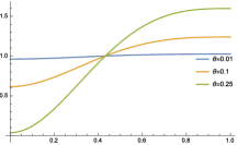
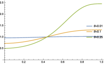
3.3 Testing arbitrary simple hypothesis

We now pass to the testing of the null hypothesis that the sample is from a continuous distribution function $F(x)$, such that $0<F(x)<1$ for all $x\in R$, against an alternative distribution function $F(x,\theta)=F(x-\theta),\;\theta>0$.

Denote the alternative density function with $f(x,\theta)$ and let $h^{\ast}(x)=f^{\prime}_{\theta}(x,0)$. If null hypothesis is true, then $F(X)$ has the uniform $U[0,1]$ distribution and the alternative that corresponds to $F(x-\theta)$ is

$$G(x,\theta)=P_{\theta}\{F(X)\leq x\}=P\{X\leq F^{-1}(x)\}=F(F^{-1}(x)-\theta),\;x\in(0,1).$$

Therefore, $G(x,\theta)$ is a close alternative to the uniform distribution, and $G(x,0)$ is obviously uniform. Then, our testing problem can be reformulated as $H_{0}:$ $U[0,1](\theta=0)$ against $H_{1}:$ $G(x,\theta)\;(\theta>0)$. The alternative density function is

$$g(x,\theta)=\frac{\partial G(x,\theta)}{\partial x}=\frac{f(F^{-1}(x),\theta)}{f(F^{-1}(x))}=\frac{f(F^{-1}(x)-\theta)}{f(F^{-1}(x))}.$$

Then we have

$$h(x)=g_{\theta}^{\prime}(x,0)=\frac{h^{\ast}(F^{-1}(x))}{f(F^{-1}(x))}.$$

Now, the integral in Theorem 3.1 can be expressed as

$$\int_{0}^{1}\int_{0}^{1}h(x)h(y)\phi^{\ast}_{m}(x,y)dxdy=\int_{0}^{1}\int_{0}^{1}\frac{h^{\ast}(F^{-1}(x))}{f(F^{-1}(x))}\frac{h^{\ast}(F^{-1}(y))}{f(F^{-1}(y))}\phi^{\ast}_{m}(x,y)dxdy$$

$$=\int_{-\infty}^{\infty}\int_{-\infty}^{\infty}\frac{h^{\ast}(u)}{f(u)}\frac{h^{\ast}(v)}{f(v)}\phi^{\ast}_{m}(F(u),F(v))f(u)f(v)dudv$$

$$=\int_{-\infty}^{\infty}\int_{-\infty}^{\infty}h^{\ast}(u)h^{\ast}(v)\phi^{\ast}_{m}(F(u),F(v))dudv.$$

Since $G(x,\theta)$ and $G(x,0)$ are defined on the same support $(0,1)$ we can calculate the Kullback-Leibler distance in terms of the Fisher information function which here is equal to

$$I =\int_{0}^{1}h^{2}(x)dx=\int_{0}^{1}\big{(}\frac{h^{\ast}(F^{-1}(x))}{f(F^{-1}(x))}\big{)}^{2}dx=\int_{-\infty}^{\infty}\big{(}\frac{h^{\ast}(u)}{f(u)}\big{)}^{2}f(u)du$$

$$=\int_{-\infty}^{\infty}\frac{(h^{\ast}(u))^{2}}{f(u)}du.$$

Therefore, we have all the ingredients to calculate the local Bahadur efficiencies of the proposed tests, in general null hypothesis case.

In Table 2, we present the local Bahadur efficiency of our tests applied to standard normal, Cauchy, and logistic null distribution and corresponding location alternatives. We use notation from [25, Ch. 2].

Table 2: Local Bahadur efficiency for location alternatives

Statistics	Gaussian	Cauchy	Logistic
$A^{2}$	0.96	0.66	1
$D$	0.64	0.81	0.75
$T^{(1)}$	0.91	0.76	0.99
$T^{(2)}$	0.87	0.72	0.95
$Q^{c}$	0	0	0
$C$	0.49	1	0.66

It is interesting to note that test (16) is locally optimal for the location alternative of Cauchy distribution.

3.4 Testing for uniformity on unknown support

In this section we show how we can adapt the presented tests to testing uniformity on an unknown support, i.e for testing $H_{0}$ that a sample $X_{1},...,X_{n}$ comes from the uniform $\mathcal{U}[a,b]$ where $a$ and $b$ are unknown.

First, consider the transformed ordered sample $Y_{2},...,Y_{n-1}$ where

$$Y_{i}=\frac{X_{(i),n}-\hat{a}}{\hat{b}-\hat{a}},\;\;i=2,3,...,n-1$$

and $\hat{a}=X_{(1),n}$ and $\hat{b}=X_{(n),n}$ are MLE of a and b, respectively.

Each of the previously presented tests can be applied to the transformed sample. Following this procedure, we obtain the tests for rectangularity on an unknown support. It is obvious that, under the null hypothesis, the distribution of test statistics does not depend on $a$ and $b$. Additionally, our statistics are symmetric functions of the sample, i.e. we may consider them as functions of order statistics. Moreover, it can be shown that random vector $(Y_{2},...,Y_{n-1})$ is equally distributed as the vector of order statistics of i.i.d. sample of size $n-2$ from uniform $\mathcal{U}[0,1]$.

Having this in mind, we conclude that all derived asymptotic properties of the proposed tests still hold.

4 Power study and applications

The powers of our and competitors tests are presented in Figures 3-10. The powers are calculated using Monte Carlo simulations with 10000 replicates at levels of significance $0.05$ and $0.1$ for samples of size $n=20$ and $n=50$.

Figure 3: Empirical powers of tests for power alternatives for $\alpha=0.05$ (left) and $\alpha=0.1$ (right), $n=20$

Figure 4: Empirical powers of tests for power alternatives for $\alpha=0.05$ (left) and $\alpha=0.1$ (right), $n=50$

Figure 5: Empirical powers of tests for $g_{2}$ alternatives for $\alpha=0.05$ (left) and $\alpha=0.1$ (right), $n=20$

Figure 6: Empirical powers of tests for $g_{2}$ alternatives for $\alpha=0.05$ (left) and $\alpha=0.1$ (right), $n=50$

Figure 7: Empirical powers of test for mixture with power alternatives for $\alpha=0.05$ (left) and $\alpha=0.1$ (right), $n=20$

Figure 8: Empirical powers of test for mixture with power alternatives for $\alpha=0.05$ (left) and $\alpha=0.1$ (right), $n=50$

Figure 9: Empirical powers of tests for Ley-Paindaveine alternatives for $\alpha=0.05$ (left) and $\alpha=0.1$ (right), $n=20$

Figure 10: Empirical powers of tests for Ley-Paindaveine alternatives for $\alpha=0.05$ (left) and $\alpha=0.1$ (right), $n=50$

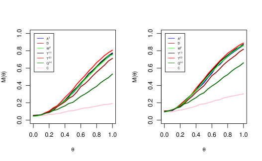
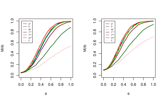
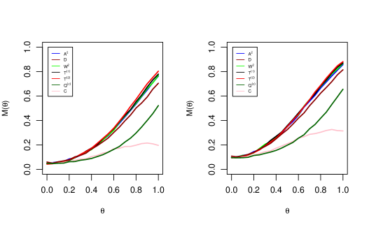
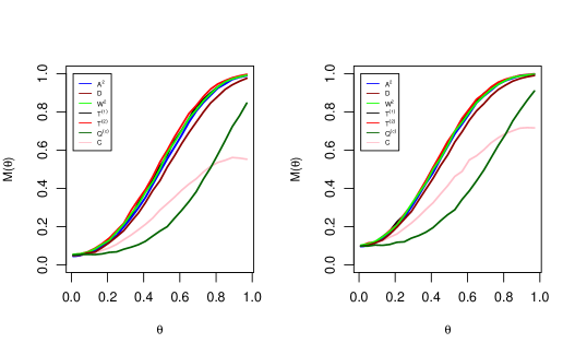
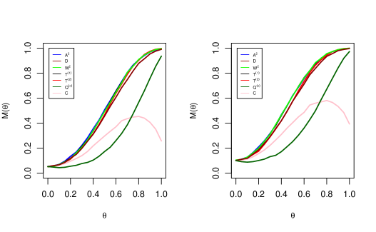
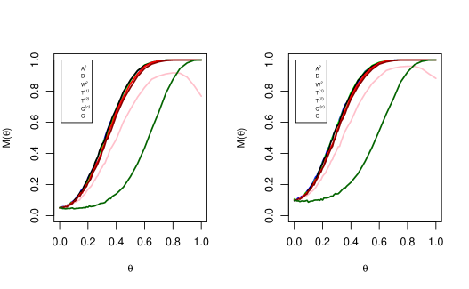
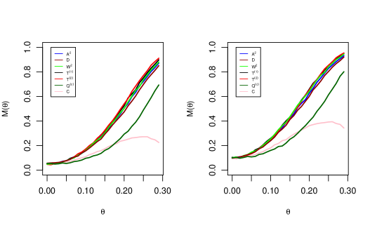
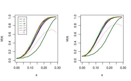
From these figures we may conclude that for all considered values of parameter $\theta$, our tests outperform the competitor ones, while the test based on the maximal covariance characterization is the worst. In particular, in the case of power and $g_{2}$ alternatives, $T^{(2)}_{n}$ is the most powerful one, while in case of other two alternatives $T^{(2)}_{n}$ and $W^{2}_{n}$ are the leading ones. Also, it is noticeable that the differences between the estimated powers of the consider tests are larger for smaller level of significance.

In order to additionally explore small sample properties of the proposed tests, we also consider the following multi-parameter alternatives defined on [0,1]:

• a beta distribution $\mathcal{B}(\alpha,\beta)$ with density

  $$g(x;\alpha,\beta)=\frac{x^{\alpha-1}(1-x)^{\beta-1}}{B(\alpha,\beta)},\;\;\alpha>0,\beta>0;$$

• a Tukey’s distribution $T(a,\lambda)$ (see [14]) with inverse d.f.

  $$G^{-1}(x;a,\lambda)=\frac{ax^{\lambda}-(1-x)^{\lambda}+1}{a+1},\;\;\;a>0,\lambda>0;$$

• a Johnson’s bounded distribution ${JB}(\frac{\gamma}{\delta^{2}},\frac{1}{\delta^{2}})$ (see [3]) with inverse d.f.

  $$G^{-1}(x;\gamma,\delta)=\frac{1}{1+e^{-\frac{\Phi^{-1}(x)-\gamma}{\delta}}},\;\;\;\gamma\in\mathbf{R},\delta>0,$$

  where $\Phi(x)$ is d.f. of standard normal distribution;

• a truncated normal distribution $TN(\mu,\sigma^{2})$ with density

  $$g(x;\mu,\sigma)=\frac{1}{(\Phi(\frac{1-\mu}{\sigma})-\Phi(\frac{-\mu}{\sigma}))\sqrt{2\pi\sigma^{2}}}e^{-\frac{(x-\mu)^{2}}{2\sigma^{2}}},\;\;\;\mu\in\mathbf{R},\sigma>0.$$

These families include both symmetric and positively and negatively skewed distributions with different shapes. One can notice that $\mathcal{B}(1,1)$ and $T(a,1)$ coincide with $\mathcal{U}[0,1]$, while $JB(\frac{\gamma}{\delta^{2}},\frac{1}{\delta^{2}})$ and $TN(\mu,\sigma^{2})$ are never uniform for any choice of parameters. The results are presented in Tables 3 and 4.

Table 3: Empirical powers of tests for $n=20$

Alternative	$\alpha$	$A^{2}$	D	$W^{2}$	$T^{(1)}$	$T^{(2)}$	$Q^{c}$	C
$\mathcal{B}(1,2)$	0.05	0.76	0.71	0.76	0.78	0.65	0.53	0.19
	0.1	0.86	0.82	0.86	0.87	0.79	0.66	0.30
$\mathcal{B}(1.2,2)$	0.05	0.49	0.48	0.51	0.54	0.33	0.49	0.11
	0.1	0.64	0.62	0.67	0.69	0.51	0.64	0.19
$\mathcal{B}(2,1.2)$	0.05	0.49	0.48	0.51	0.54	0.61	0.49	0.11
	0.1	0.65	0.63	0.67	0.70	0.74	0.64	0.19
$\mathcal{B}(1.2,0.8)$	0.05	0.34	0.29	0.32	0.33	0.30	0.09	0.15
	0.1	0.46	0.40	0.45	0.45	0.41	0.15	0.23
$\mathcal{B}(3,2)$	0.05	0.47	0.53	0.49	0.57	0.71	0.89	0.04
	0.1	0.68	0.68	0.70	0.76	0.85	0.95	0.10
$\mathcal{B}(0.5,0.5)$	0.05	0.54	0.21	0.19	0.16	0.16	0.24	0.21
	0.1	0.66	0.33	0.33	0.27	0.26	0.40	0.28
$T(2,3)$	0.05	0.23	0.26	0.25	0.27	0.18	0.24	0.17
	0.1	0.35	0.38	0.38	0.40	0.32	0.34	0.27
$T(3,2)$	0.05	0.28	0.23	0.24	0.24	0.23	0.07	0.16
	0.1	0.38	0.33	0.35	0.34	0.36	0.12	0.24
$T(0.5,3.5)$	0.05	0.29	0.36	0.33	0.36	0.41	0.37	0.23
	0.1	0.43	0.47	0.48	0.51	0.53	0.49	0.35
$T(1,10)$	0.05	0.85	0.85	0.87	0.92	0.82	0.99	0.71
	0.1	0.95	0.94	0.97	0.98	0.92	0.99	0.86
$JB(0.5,0.5)$	0.05	0.69	0.60	0.63	0.62	0.65	0.10	0.45
	0.1	0.78	0.70	0.73	0.72	0.75	0.15	0.55
$JB(-0.5,0.5)$	0.05	0.69	0.60	0.62	0.62	0.54	0.10	0.44
	0.1	0.78	0.71	0.73	0.72	0.63	0.15	0.53
$JB(0.5,1)$	0.05	0.46	0.51	0.49	0.57	0.21	0.90	0.05
	0.1	0.67	0.67	0.68	0.75	0.44	0.95	0.11
$JB(-0.5,1)$	0.05	0.46	0.52	0.49	0.59	0.69	0.90	0.05
	0.1	0.67	0.67	0.69	0.76	0.83	0.95	0.12
$JB(0,0.5)$	0.05	0.11	0.10	0.09	0.07	0.07	0.02	0.10
	0.1	0.18	0.16	0.15	0.13	0.13	0.06	0.15
$TN(1,0.5^{2})$	0.05	0.58	0.56	0.58	0.62	0.63	0.36	0.22
	0.1	0.71	0.67	0.71	0.73	0.74	0.48	0.34
$TN(1.2,0.5^{2})$	0.05	0.85	0.82	0.86	0.87	0.88	0.57	0.34
	0.1	0.92	0.90	0.93	0.93	0.93	0.69	0.47
$TN(0.5,0.2^{2})$	0.05	0.19	0.20	0.16	0.28	0.24	0.94	0.04
	0.1	0.45	0.39	0.42	0.56	0.47	0.97	0.11

Table 4: Empirical powers of tests for $n=50$

Alternative	$\alpha$	$A^{2}$	D	$W^{2}$	$T^{(1)}$	$T^{(2)}$	$Q^{c}$	C
$\mathcal{B}(1,2)$	0.05	0.99	0.98	1	1	0.98	0.88	0.53
	0.1	1	0.99	1	1	0.99	0.94	0.71
$\mathcal{B}(1.2,2)$	0.05	0.94	0.90	0.94	0.94	0.81	0.87	0.32
	0.1	0.98	0.95	0.97	0.97	0.92	0.93	0.47
$\mathcal{B}(2,1.2)$	0.05	0.94	0.91	0.93	0.94	0.97	0.87	0.32
	0.1	0.97	0.95	0.97	0.97	0.99	0.93	0.47
$\mathcal{B}(1.2,0.8)$	0.05	0.70	0.58	0.66	0.66	0.63	0.12	0.35
	0.1	0.79	0.70	0.77	0.76	0.74	0.19	0.46
$\mathcal{B}(3,2)$	0.05	0.98	0.96	0.98	0.99	1	1	0.15
	0.1	1	0.99	0.99	1	1	1	0.30
$\mathcal{B}(0.5,0.5)$	0.05	0.87	0.43	0.45	0.40	0.40	0.84	0.42
	0.1	0.94	0.60	0.66	0.58	0.55	0.91	0.54
$T(2,3)$	0.05	0.55	0.57	0.59	0.61	0.49	0.40	0.45
	0.1	0.69	0.69	0.72	0.72	0.66	0.52	0.58
$T(3,2)$	0.05	0.54	0.46	0.52	0.52	0.54	0.07	0.35
	0.1	0.66	0.58	0.64	0.64	0.66	0.13	0.46
$T(0.5,3.5)$	0.05	0.71	0.74	0.75	0.76	0.80	0.66	0.63
	0.1	0.83	0.83	0.86	0.86	0.88	0.76	0.75
$T(1,10)$	0.05	1	1	1	1	1	1	1
	0.1	1	1	1	1	1	1	1
$JB(0.5,0.5)$	0.05	0.97	0.93	0.95	0.95	0.96	0.11	0.84
	0.1	0.98	0.96	0.97	0.97	0.98	0.17	0.89
$JB(-0.5,0.5)$	0.05	0.96	0.93	0.95	0.95	0.90	0.11	0.83
	0.1	0.98	0.96	0.98	0.97	0.94	0.17	0.89
$JB(0.5,1)$	0.05	0.98	0.96	0.97	0.98	0.79	1	0.18
	0.1	0.99	0.98	0.99	0.99	0.94	1	0.33
$JB(-0.5,1)$	0.05	0.99	0.96	0.97	0.98	0.99	1	0.19
	0.1	1	0.99	0.99	1	1	1	0.35
$JB(0,0.5)$	0.05	0.14	0.11	0.10	0.09	0.09	0.12	0.13
	0.1	0.24	0.20	0.19	0.17	0.18	0.22	0.22
$TN(1,0.5^{2})$	0.05	0.94	0.92	0.95	0.95	0.96	0.67	0.61
	0.1	0.97	0.97	0.98	0.98	0.98	0.77	0.74
$TN(1.2,0.5^{2})$	0.05	1	1	1	1	1	0.89	0.82
	0.1	1	1	1	1	1	0.94	0.90
$TN(0.5,0.2^{2})$	0.05	0.93	0.75	0.86	0.92	0.84	0.99	0.21
	0.1	0.99	0.90	0.97	0.98	0.96	1	0.44

Taking into account the previous results, and those presented in Tables 3 and 4, we may conclude that, although asymptotically equivalent, the tests $T_{n}^{(1)}$ and $W^{2}_{n}$ do differ for small sample size $n=20$. Moreover, in that case, $T_{n}^{(1)}$ is usually more powerful than $W^{2}_{n}$.

In general, for the sample size $n=20$, the ”ordering” of the considered tests largely depends on the shape of the alternative distribution. In particular, for alternatives with monotone densities, the classical tests $A^{2}_{n},D_{n},W^{2}_{n}$, and our two tests $T^{(1)}_{n}$ and $T^{(2)}_{n}$ are shown to be much more powerful than $Q^{c}_{n}$ and $C.$ Usually $T^{(2)}_{n}$ is the leading one. Also, $T^{(1)})n$ and $T^{(2)}_{n}$ are among the best, for positively and negatively skewed alternatives, respectively, and the only test that is sometimes better in these cases is $Q^{c}_{n}$. In the case of U-shaped densities, $A^{2}_{n}$ is the leading one. For the grater sample size $n=50$, the ”ordering” of the tests is very similar.

4.1 Specification tests for conditional duration models

Recently, high-frequency data have become widely available in markets. Therefore, there is a growing interest in modeling such data with special attention given to modeling the times between observations. [8] and [6], using the idea from GARCH, proposed to model durations (appropriately standardized) with

$$x_{t}=\mu_{t}\varepsilon_{t},\ \mu_{t}=a_{0}+\sum_{j=1}^{p}a_{j}x_{t-j}+\sum_{j=1}^{q}b_{j}\tilde{\mu}_{t-j},$$

where $\varepsilon_{t}$ is a sequence of i.i.d. positive random variables with d.f. F and the expectation one, so called innovation process. This model is widely known as Autoregressive Conditional Duration Model and labeled with ACD(p,q). Naturally, developing modeling diagnostic tools have become important. One of two possible directions is to inspect the adequacy of the functional form of the conditional duration, while the other is to test the distribution of the error term.

In this section we compare the introduced tests as the specification tests for ACD model with exponential innovations ($\rm EACD$ model). Since the innovations are unobservable, it is natural to base a test on corresponding residuals given by

$$\widehat{\varepsilon}_{t}=\frac{x_{t}}{\widehat{\mu}_{t}},\;t=1,...,T,$$

where $\widehat{\mu}_{t}$ is the estimator of conditional mean duration. Taking into account the model definition, the null hypothesis is that the corresponding innovations have exponential $\mathcal{E}(1)$ distribution. Hence, we apply our tests to the appropriately transformed residuals. Following the procedure described in [19], we obtain the empirical powers of considered tests. In order to use results from [19] as benchmark ones, we consider $ACD(1,1)$ model with parameters $a_{0}=0.3,a_{1}=0.3$ and $b_{1}=0.4$ and sample sizes $T=100$ and $T=200$. For alternative distribution we choose Weibull, gamma and lognormal distributions (see [19]).

From Tables 5 and 6 and the results presented in [19], we can notice that all empirical sizes are satisfactory and that, in general, the powers are reasonably high for all tests. In particular, in the case of gamma and Weibull alternative, tests based on Too-Lin characterization are among the best. They are more powerful than $C_{n}$, $Q^{c}_{n}$, and classical $D_{n}$ tests and comparable with $A^{2}_{n}$ and $W^{2}_{n}$ tests. A similar situation is in the case of lognormal alternative with the exception of $C_{n}$ that outperforms others for shape parameter $\theta=1.1$.

Table 5: Empirical powers of tests for exponential innovations, for $T=100$

Alternative	$A^{2}$	D	$W^{2}$	$T^{(1)}$	$T^{(2)}$	$Q^{C}$	C
E(1)	0.06	0.06	0.06	0.05	0.06	0.05	0.04
W(1.1)	0.24	0.18	0.20	0.22	0.23	0.21	0.10
W(1.2)	0.56	0.46	0.54	0.57	0.56	0.57	0.19
W(1.3)	0.88	0.78	0.85	0.87	0.87	0.83	0.33
W(1.4)	0.98	0.95	0.98	1	1	0.98	0.50
W(1.5)	1		1	1	1	1	0.67
G(1.2)	0.25	0.20	0.24	0.23	0.25	9.30	0.10
G(1.3)	0.44	0.39	0.42	0.46	0.48	0.51	0.13
G(1.4)	0.70	0.52	0.65	0.63	0.65	0.71	0.17
G(1.5)	0.81	0.71	0.78	0.78	0.81	0.84	0.23
LN(0.8)	1	0.97	0.98	0.99	1	1	0.27
LN(0.9)	0.89	0.69	0.73	0.81	0.87	0.3	0.34
LN(1)	0.65	0.41	0.49	0.51	0.55	0.62	0.46
LN(1.1)	0.58	0.49	0.54	0.55	0.51	0.20	0.65

Table 6: Empirical powers of tests for exponential innovations, for $T=200$

Alternative	$A^{2}$	D	$W^{2}$	$T^{(1)}$	$T^{(2)}$	$Q^{c}$	C
E(1)	0.05	0.06	0.05	0.04	0.04	0.04	0.05
W(1.1)	0.33	0.31	0.33	0.36	0.37	0.35	0.15
W(1.2)	0.86	0.75	0.85	0.86	0.86	0.84	0.40
W(1.3)	1	0.97	1	1	1	0.99	0.66
W(1.4)	1	1	1	1	1	1	0.86
G(1.2)	0.47	0.34	0.42	0.43	0.47	0.48	0.13
G(1.3)	0.75	0.62	0.71	0.72	0.76	0.77	0.21
G(1.4)	0.96	0.83	0.93	0.90	0.91	0.93	0.32
G(1.5)	0.99	0.94	0.97	0.97	0.98	0.99	0.45
LN(0.8)	1	1	1	1	1	1	0.26
LN(0.9)	1	0.98	0.99	0.99	1	1	0.69
LN(1)	0.98	0.77	0.89	0.92	0.92	0.89	0.81
LN(1.1)	0.95	0.81	0.90	0.91	0.88	0.37	0.93

4.2 Detecting hidden periodicity

We shall demonstrate the use of the cumulative periodogram as a useful diagnostic tool for hidden periodicity of the unspecified frequencies. For more on theory of analysis of time series in frequency domain we refer to [4].

Let us consider a real-valued stationary time series $\{X_{t},\;t\geq 0\}$, and let $f(\omega_{i})$ and $I(\omega_{i})$ be the corresponding spectral density of $X_{t}$ and its estimate based on the first $n$ elements of $X_{t}$, evaluated at Fourier frequencies $\omega_{i}=2\pi i/n$. In [4] it is proved that $\{X_{t},0\leq t\leq n\}$ is Gaussian white noise if and only if the random variables

$$Y_{k}=\frac{\sum_{i=1}^{k}I(\omega_{i})}{\sum_{i=1}^{q-1}I(\omega_{i})},\;\;k=1...q-1,\;\;q=\Big{[}\frac{n-1}{2}\Big{]},$$

are distributed as the order statistics from uniform $\mathcal{U}[0,1]$ distribution. Hence, we can use the uniformity tests to check whether $\{X_{t}\}$ is Gaussian white noise.

We compare the powers of presented tests for artificially generated time series

$$X_{t}=\sin\frac{\pi t}{a}+Z_{t},\;t=1...T,$$ (23)

where $\{Z_{t}\}$ is Gaussian white noise. The powers are estimated based on $N=10000$ Monte Carlo replicates and for level of significance $\alpha=0.05$, for different values of parameter $a$. The values are given in Tables 7 and 8.

$a$	$A^{2}$	$D$	$W^{2}$	$T^{(1)}$	$T^{(2)}$	$Q^{c}$	$C$
$\infty$	0.07	0.07	0.07	0.06	0.07	0.05	0.07
1	0.07	0.06	0.06	0.06	0.06	0.05	0.07
2	0.63	0.67	0.57	0.49	0.50	0.65	0.91
3	0.70	0.77	0.68	0.64	0.64	0.23	0.94
4	0.78	0.85	0.79	0.78	0.80	0.00	0.96
5	0.85	0.91	0.87	0.86	0.90	0.02	0.97
6	0.88	0.92	0.89	0.89	0.92	0.13	0.97
7	0.91	0.94	0.92	0.92	0.95	0.40	0.97
8	0.91	0.95	0.93	0.92	0.96	0.61	0.97
9	0.92	0.96	0.93	0.94	0.96	0.74	0.96
10	0.95	0.97	0.95	0.95	0.98	0.84	0.96

Table 7: Empirical powers in case of testing for hidden periodicities, for $T=100$

$a$	$A^{2}$	$D$	$W^{2}$	$T^{(1)}$	$T^{(2)}$	$Q^{c}$	$C$
$\infty$	0.06	0.07	0.07	0.07	0.06	0.06	0.07
1	0.07	0.07	0.06	0.07	0.06	0.05	0.07
2	0.96	0.98	0.97	0.96	0.94	0.95	1.00
3	0.97	0.99	0.97	0.97	0.98	0.65	1.00
4	0.99	0.99	0.99	0.99	0.99	0.02	1.00
5	0.99	1.00	1.00	1.00	1.00	0.02	1.00
6	1.00	1.00	1.00	1.00	1.00	0.25	1.00
7	1.00	1.00	1.00	1.00	1.00	0.63	1.00
8	1.00	1.00	1.00	1.00	1.00	0.85	1.00
9	1.00	1.00	1.00	1.00	1.00	0.94	1.00
10	1.00	1.00	1.00	1.00	1.00	0.97	1.00

Table 8: Empirical powers in case of testing for hidden periodicities, for $T=200$

We notice that our tests perform well in all cases, while the test based on maximal correlation is the worst one, and, surprisingly, the test based on maximal covariance characterization outperformed the others. The similar conclusion is for the series of size 200. In many cases, the power are very high, and the ”ordering” for each value of $a$ is the same.

References

- [1] P. Anand. Characterizations of the uniform distribution via sample spacings and nonlinear transformations. J. Math. Anal. Appl., 284(1):397–402, 2003.
- [2] R. R. Bahadur. Some limit theorems in statistics. SIAM, 1971.
- [3] K O. Bowman and L. R. Shenton. Johnson’s system of distributions. In Encyclopedia of Statistical Sciences, volume 4, pages 303–314. John Wiley & Sons, 1983.
- [4] P. J. Brockwell and R. A. Davis. Time series: theory and methods. Springer Science & Business Media, 2013.
- [5] R. B. D’Agostino. Goodness-of-fit-techniques, volume 68. CRC press, 1986.
- [6] A. Dufour and R. F. Engle. Time and the price impact of a trade. J. Finance, 55(6):2467–2498, 2000.
- [7] K.O. Dzhaparidze and M.S. Nikulin. Probability distributions of the kolmogorov and omega-square statistics for continuous distributions with shift and scale parameters. J. Math. Sci., 20(3):2147–2164, 1982.
- [8] R. F. Engle and J. R. Russell. Autoregressive conditional duration: a new model for irregularly spaced transaction data. Econometrica, pages 1127–1162, 1998.
- [9] J. Fortiana and A. Grané. Goodness-of-fit tests based on maximum correlations and their orthogonal decompositions. J. R. Stat. Soc. Ser. B Stat. Methodol., 65(1):115–126, 2003.
- [10] J. Galambos and S. Kotz. Characterization of Probability Distributions. Springer-Verlag, Berlin-Heidelberg-New York, 1978.
- [11] M. N. Goria. Some characterizations of the uniform distribution. Comm. Statist. Theory Methods, 16(3):813–819, 1987.
- [12] A. Grané and A. V. Tchirina. Asymptotic properties of a goodness-of-fit test based on maximum correlations. Statistics, 47(1):202–215, 2013.
- [13] T. Hashimoto and S. Shirahata. A Goodness of Fit Test Based on a Characterization of Uniform Distribution. J. Japan Statist. Soc., 23(2):123–130, 1993.
- [14] B. L. Joiner and J. R. Rosenblatt. Some properties of the range in samples from tukey’s symmetric lambda distributions. J. Am. Stat. Assoc., 66(334):394–399, 1971.
- [15] M. Jovanović, B. Milošević, Ya. Yu. Nikitin, M. Obradović, and K. Yu. Volkova. Tests of exponentiality based on Arnold–Villasenor characterization and their efficiencies. Comput. Stat. Data Anal., 90:100–113, 2015.
- [16] E. Kamke. Differentialgleichungen. Losungsmethoden und Losungen I 7th edition. Akademische Verlagsgesellschaft Geest and Porting K.-G., Leipzig,, 1961.
- [17] V. S. Korolyuk and Yu. V. Borovskikh. Theory of U-statistics. Kluwer, Dordrecht, 1994.
- [18] C. Ley and D. Paindaveine. Le Cam optimal tests for symmetry against Ferreira and Steel’s general skewed distribution. J. Nonparametr. Stat., 21(8):943–967, 2008.
- [19] S. G. Meintanis, B. Milošević, and M. Obradović. Goodness-of-fit tests in conditional duration models. Statist. Papers, pages 1–18, 2017.
- [20] B. Milošević. Asymptotic efficiency of new exponentiality tests based on a characterization. Metrika, 79(2):221–236, 2016.
- [21] B. Milošević and M. Obradović. New class of exponentiality tests based on U-empirical Laplace transform. Statist. Papers, 57(4):977–990, 2016.
- [22] B. Milošević and M. Obradović. Two-dimensional Kolmogorov-type goodness-of-fit tests based on characterisations and their asymptotic efficiencies. J. Nonparametr. Stat., 28(2):413–427, 2016.
- [23] K. W. Morris and D. Szynal. Goodness-of-fit tests based on characterizations of continuous distributions. Appl. Math., 27(4):475–488, 2000.
- [24] K. W. Morris and D. Szynal. Goodness-of-fit tests using dual versions of characterizations via moments of order statistics. J. Math. Sci., 122(4):3365–3383, 2004.
- [25] Ya. Yu. Nikitin. Asymptotic efficiency of nonparametric tests. Cambridge University Press, New York, 1995.
- [26] Ya. Yu. Nikitin and I. Peaucelle. Efficiency and local optimality of nonparametric tests based on U- and V-statistics. Metron, 62(2):185–200, 2004.
- [27] Ya. Yu. Nikitin and E. V. Ponikarov. Rough large deviation asymptotics of Chernoff type for von Mises functionals and U-statistics. Proceedings of Saint-Petersburg Mathematical Society, 7:124–167, 1999. English translation in AMS Translations, ser. 2, 203:107–146, 2001.
- [28] Ya. Yu. Nikitin and K. Yu. Volkova. Asymptotic efficiency of exponentiality tests based on order statistics characterization. Georgian Math. J., 17(4):749–763, 2010.
- [29] M. Obradović. On asymptotic Efficiency of Goodness of Fit Tests for Pareto Distribution Based on Characterizations. Filomat, 29(10):2311–2324, 2015.
- [30] M. Obradović, M. Jovanović, and B. Milošević. Goodness-of-fit tests for Pareto distribution based on a characterization and their asymptotics. Statistics, 49(5):1026–1041, 2015.
- [31] V. Papathanasiou. Some characterizations of distributions based on order statistics. Statist. Probab. Lett., 9(2):145–147, 1990.
- [32] C. Tenreiro. On the finite sample behavior of fixed bandwidth Bickel–Rosenblatt test for univariate and multivariate uniformity. Comm. Statist. Simulation Comput., 36(4):827–846, 2007.
- [33] Y. H. Too and G. D. Lin. Characterizations of uniform and exponential distributions. Statist. Probab. Lett., 7(5):357–359, 1989.
- [34] H. Volkmer and G. G. Hamedani. On distributions of order statistics and their applications to uniform distribution. Metrika, 74(2):287–295, 2011.