Features of electroweak symmetry breaking in five dimensional SUSY models
Abstract
We explore the phenomenological predictions of a supersymmetric standard model, with a large extra dimension and unifying gauge couplings. The modified five dimensional renormalisation group equations make it possible to obtain light, maximally mixed stops, with a low scale of supersymmetry breaking and a low unification scale. This allows the fine-tuning to be lowered right down to the barrier coming directly from experimental lower limits on the stop masses. We also show that modifying the SUSY breaking pattern to obtain lighter stops at the high scale does not result in fine-tuning relaxation, and only RGE effects turn out to be effective in generating a lower fine-tuning.
Keywords:
Large A-term, extra dimension, light third-generation squarks1 Introduction
The discovery of the Higgs boson, of mass GeV, at the first LHC run Aad:2012tfa ; Chatrchyan:2012ufa and various null results in searches for super-particles (sparticles) appear to imply that the sparticles of minimal theories of supersymmetry (such as the MSSM) are likely to be out of reach of the LHC altogether. Further considerations regarding electroweak symmetry breaking and the naturalness aesthetic bring further doubt that perhaps supersymmetry is not a symmetry of nature after all.
At this time it is also worth to consider non minimal models that share much of the well grounded theoretical elegance of the (four dimensional) MSSM: supersymmetry, gauge coupling unification, anomaly cancellation, a minimal matter content to achieve these, unification of matter representations, an explanation of the big hierarchy problem, various dark matter candidates. The model we consider is five dimensional and brings with it additional interesting features: the possibility to observe Kaluza-Klein states of gauge (and other) fields Antoniadis:1990ew , the possibility to achieve the observed Higgs mass with sparticles within reach of the next LHC run, and a much lower unification scale and supersymmetry breaking scale than is normally possible in four dimensions.
In this paper we explore electroweak symmetry breaking in a particular class of five dimensional supersymmetric theories Pomarol:1998sd ; Abdalgabar:2015ora . We also wish to address the possibility to construct a ‘natural theory’ where stops are lighter than their first and second generation counterparts, and which is not spoiled by the renormalisation group effects that would usually make the 3rd generation similarly heavy at a low scale, after a long period of RG-running. Studying models that differ in how matter fields are located among branes and bulk opens the possibility to explore the effect different SUSY breaking patterns and modified five dimensional RGEs have on fine-tuning wrt a four dimensional theory. Unfortunately modifying the breaking pattern to obtain more natural soft terms at the high scale does not give the expected fine-tuning relaxation. However we show that modified RGEs enable us to obtain light maximally mixed stops. This allows us to lower fine-tuning down to the barrier coming directly from observational lower limits on the stop mass.
In our analysis we used renormalisation group equations outlined in Abdalgabar:2014bfa ; Abdalgabar:2015ora and adapted a C++ based spectrum generator originally intended for the (four dimensional) MSSM Lalak:2013bqa . A similar modification may be carried out with any publicly available spectrum generator Allanach:2001kg ; Porod:2003um ; Djouadi:2002ze 111To date, five dimensional theories are one such class of models that cannot yet be explored using SARAH Staub:2009bi ; Staub:2010jh ; Staub:2012pb ; Staub:2013tta although it can still be a powerful tool to determine the RGEs of the low energy four dimensional effective theory that the five dimensional theory runs to Abdalgabar:2015ora .. The RGEs used in this paper may be found in Abdalgabar:2015ora and further conventions in Abdalgabar:2014bfa and Hebecker:2001ke ; Mirabelli:1997aj ; McGarrie:2010kh ; Cornell:2011fw ; McGarrie:2013hca . For earlier phenomenological studies of five dimensional theories see for example Bhattacharyya:2010rm .
The outline of the paper is as follows: section 2 we outline the two base models that we wish to explore. In section 3 we explore the behaviour of the running parameters of the theories. In section 5 we look at naturalness and electroweak symmetry breaking as we vary the radius of the extra dimension. We also look at benchmark models of supersymmetry breaking in section 4. In section 4.3 we outline and explore a “natural” model in which the 3rd generation are spatially located on a different brane to the first two generations and in which supersymmetry is gauge mediated directly to the first two generations but only indirectly to the 3rd, which ideally would allow for light stops. In section 6 we conclude. In appendix A we outline the implementation of spectrum generator and RG solver in C++ code.
2 The 5D-SSM+ Model
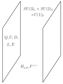
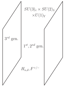
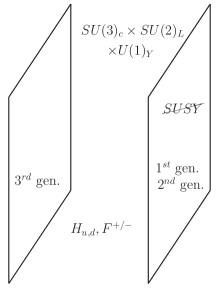
The first model that we wish to explore is a five dimensional supersymmetric theory with the field content outlined in table 1 and is pictured in figure 1 (left). In this model the Higgs fields (), gauge fields and additionally are bulk fields Delgado:1998qr . This matter content is necessary for the gauge couplings unification, as we shall explore further later. All five dimensional bulk matter fields are supersymmetric Hypermultiplets which due to even and odd boundary conditions lead to a four dimensional Chiral multiplet as a zero mode of the Kaluza-Klein expansion: such details are well documented, for instance in Hebecker:2001ke ; Mirabelli:1997aj ; McGarrie:2010kh ; Cornell:2011fw ; McGarrie:2013hca . The second model we wish to explore is outlined in table 2 and pictured in figure 1 (right). In model 2 only the third generation is located on a brane and the first and second generation are in the bulk along with the Higgs multiplets and fields.
| Superfields | Brane | Bulk | |
| ✓ | - | ||
| ✓ | - | ||
| ✓ | - | ||
| ✓ | - | ||
| ✓ | - | ||
| - | ✓ | ||
| - | ✓ | ||
| - | ✓ | ||
| - | ✓ | ||
| - | ✓ | ||
| - | ✓ | ||
| - | ✓ |
| Superfields | Brane | Bulk | |
| - | ✓ | ||
| - | ✓ | ||
| - | ✓ | ||
| - | ✓ | ||
| - | ✓ | ||
| ✓ | - | ||
| ✓ | - | ||
| ✓ | - | ||
| ✓ | - | ||
| ✓ | - | ||
| - | ✓ | ||
| - | ✓ | ||
| - | ✓ | ||
| - | ✓ | ||
| - | ✓ | ||
| - | ✓ | ||
| - | ✓ |
The superpotential for both models is given by
| (1) |
It would be very worthwhile to consider the generation of the term in the superpotential, although for this paper we will not need to consider it, and postpone that to later work. We will now explore the running parameters of these two theories as one changes the scale of the extra dimension.
3 Running parameters
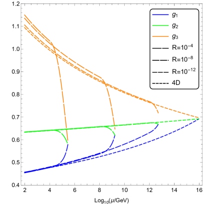
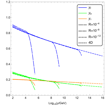
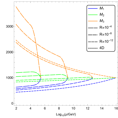
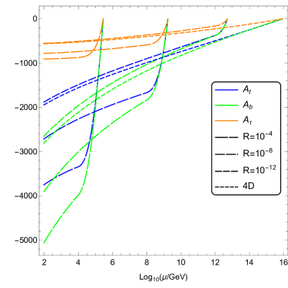
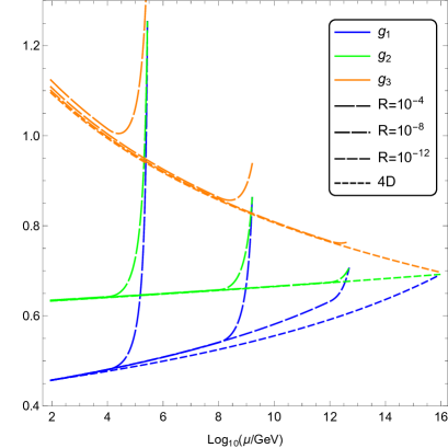
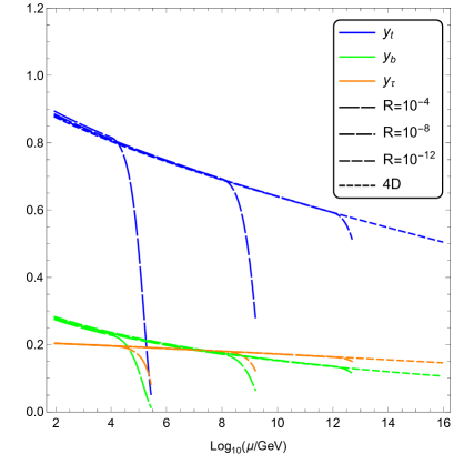
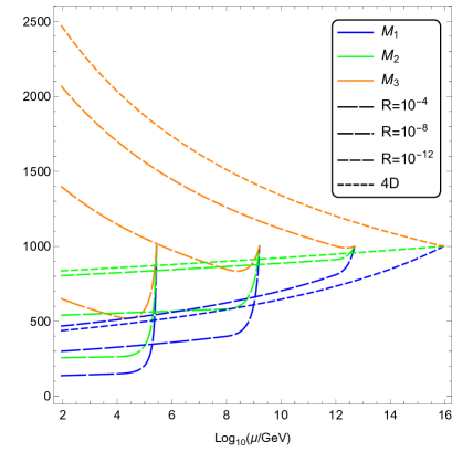
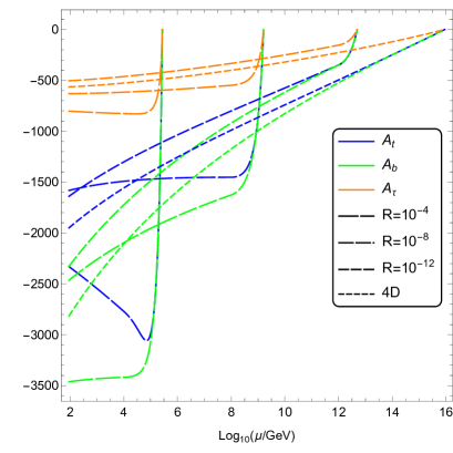
It is particularly interesting to understand and compare the behaviour of the various running parameters of these theories compared to the more usual four dimensional MSSM. The behaviour of the various parameters as a function of renormalisation scale for model 1 is pictured in figure 2. Of particular note is that unification happens much earlier if the size of the extra dimension is large Dienes:1998vg , than the usual four dimensional case. One also finds that the top Yukawa reduces rather significantly and becomes of similar order to the other Yukawa couplings near the unification scale. In addition one finds that even for initially vanishing A-terms the term may become multi-TeV in value at the electoweak scale, which is encouraging from the perspective of obtaining the observed Higgs mass. It is also the case (bottom left) that the gluino mass can become much hearvier than the other gauginos allowing for the theory to still have a light bino and wino whilst allowing for a gluino above current exclusions.
The first model may be compared with model 2 similarly presented in figure 3 and in table 2. In these figures it is notable that that gauge couplings quite nearly unify but the gauge couplings rise rather than fall, after the KK modes start to take effect in the RGEs. The still decreases in value, although now rather interestingly the becomes so quickly negative that it can quickly overcompensate the effect of the gluino soft mass, and for very large radius, the running may even return on itself. Again the wino and bino soft terms can be much smaller than that of the gluino, even starting from the same initial value.
4 Supersymmetry breaking in benchmark models
So far our exploration has been reasonably agnostic about how supersymmetry is broken, since the main feature of the models presented in the previous sections are their RGEs. In what follows we will simply refer to sets of RGEs we used, as models.
There are however a number of ways that have been proposed for the parametrisation of supersymmetry breaking in a five dimensional scenario. In this section we wish to identify these scenarios and look at their patterns of supersymmetry breaking which define their possible high scale spectra.
4.1 Gravity mediation (CMSSM)
Our first benchmark scenario is the simple CMSSM spectrum, however since easier generation of -terms during running is a key feature of five dimensional running, we will always take case for which the difference between five and four dimensional theories is the most visible. This implies a very simple type of spectrum with just two free parameters and :
| (2) |
defined at the unification scale.
4.2 Minimal Gauge Mediation (MGM) in five dimensions
In gauge mediation there is an additional characteristic scale at which SUSY is broken, which for brevity we will labelled . For the five dimensional RGEs to have an impact on the spectrum and to not simply be an effective four dimensional theory with a low SUSY breaking scale we wish that M is at least and possibly nearer .
The soft terms in five dimensional GMSB, at the breaking scale, are then given by
| (3) |
where and are the free parameters we will scan over. This paper is the first implementation of five dimensional GMSB soft masses Kaplan:1999ac ; Chacko:1999mi ; Mirabelli:1997aj ; McGarrie:2010kh ; McGarrie:2011av , with five dimensional RGEs Abdalgabar:2015ora ; Abdalgabar:2014bfa . In both model 1 and 2 we will take the supersymmetry breaking to be on the opposite brane to the matter, and both brane and bulk matter are essentially suppressed by the effect of the extra dimension, as in the above equation.
4.3 Realising natural SUSY with GMSB in five dimensions (nMGM)
The renormalisation group equations of model 1 may be used to explore a natural susy scenario as pictured in figure 4. In this model the 3rd generation is located on one brane and the 1st and 2nd generation on another, along with the supersymmetry breaking sector. The effects of supersymmetry breaking are mediated by gauge forces Giudice:1998bp (but one can also easily consider gravity mediation too in this context) and the result is that the 1st and 2nd generation and also the gauginos will receive normal (4D) GMSB soft mass contributions but the 3rd generation will be heavily suppressed McGarrie:2011av ; McGarrie:2010kh ; Abdalgabar:2014bfa ; Abdalgabar:2015ora . The soft mass matrix for squarks and sleptons takes the form
| (4) |
leading to an interesting natural SUSY spectrum of lighter 3rd generation squarks. This scenario suggests that natural SUSY softer terms are imprinted due to the ‘geometry’ of the theory. We will consider such a natural spectrum in context of minimal gauge mediation, the resulting soft terms are similar to those in(3), however now only third generation sfermions are suppressed by . In the text we will refer to this as an nMGM spectrum. Needless to say, a similar model may be constructed using brane to brane gravity mediation. It would also be interesting to discuss models with and localised alongside the 3rd families, however it would require a much more serious modification of the RGE’s of our Model 1 and 2, consequently we postpone that discussion to future work.
5 Electroweak symmetry breaking and naturalness
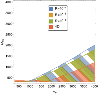
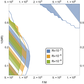
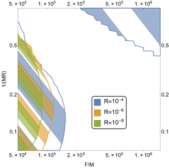
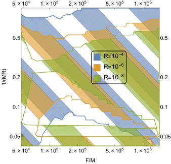
One important feature of a model is whether its parameter space can accommodate electroweak symmetry breaking. Figure 5 shows regions in the parameter space of our models where the breaking does not occur or which violate direct detection bounds summarised in table 3 Agashe:2014kda . Exclusions corresponding to varying size of the extra dimension (including the case) are plotted together.
| particle | mass bound in GeV |
|---|---|
For standard CMSSM and MGM boundary conditions Model predicts rather standard spectra of sparticles quite similar to the case. However Model 2 due to much lower gaugino masses compared to the -terms allows us to obtain very light stops and maximal mixing even despite -terms vanishing at the unification scale. In fact for large the peculiar shape of the CMSSM excluded region in model 2 comes from obtaining too light stops that would have already been observed.
The MGM excluded region comes from the interplay between large scalar masses we obtain at the scale when , and when they are generated during 5D modified running between and . The minimal stop mass is obtained between these two situations and results in excluded part on the left hand side of middle row in Figure 5 where the small stop soft mass fails to push to negative values and break electroweak symmetry.
This is also visible in nMGM plot on the bottom row of Figure 5. However here the problem is more severe since is not suppressed by at the SUSY breaking scale, and a much bigger part of the parameter space is excluded. For nMGM spectrum this problem appears also for very small , because in this part of the parameter space the difference between Higgs and stop soft masses is the largest. These two effects lead to appearance of a window of allowed parameter space which is very interesting, since it is in that window, that we obtain the highest Higgs mass.

5.1 Exploring naturalness in benchmark scenarios
In MSSM-like theories, at a finite loop order, electroweak symmetry breaking is radiatively induced. The up-Higgs soft mass is driven to negative values, leading to
| (5) |
At leading order, the running of this soft mass in four dimensions follows
| (6) |
In five dimensional models the RGEs are rather different due to the power law contributions and one finds
| (7) |
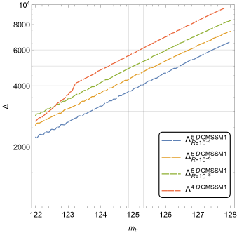
One might have expected a significant contribution to fine tuning from the power law contribution. However four and five dimensional theories actually have similar fine tuning as the much faster power law contribution can dominate the running for only a very small range of scales if the spectra we are comparing are similar. And so the final amount of fine-tuning for a given scenario depends mostly on the resulting spectrum rather than on the amount of power law running. This is quantified in figure 6, where in numerical calculations we use a standard fine-tuning measure with respect to parameter defined as follows222The numerical procedure used to calculate fine-tuning is detailed in appendix A.5. Ellis:1985yc ; Barbieri:1987fn ; Chankowski:1998xv
| (8) |
Fine-tuning connected with a set of independent parameters is then
| (9) |
Figure 6 shows resulting fine-tuning as a function of Higgs mass for different sizes of the extra dimension as well as the result one would obtain from running. the top row shows results obtained assuming CMSSM-like soft terms (with ), the middle row shows gauge mediated boundary conditions and the bottom plot shows the nMGM ones.
The results in left panel show model which gives a rather standard prediction despite power law contribution to running. However model shown on the right hand side allows us to reduce fine-tuning very significantly. The reason are the gaugino masses that decrease during 5D part of the running (as shown in Figure 3). This protects the soft terms from the usual increase due to the heavy gluino. Since the A-terms do not grow proportionally to scalar masses we can easily achieve maximal mixing scenario for the light stops, and their direct detection bound is precisely what gives us the lower bound on fine-tuning we can see in model with .
The bottom plot shows nMGM result which turns out quite similar to MGM and CMSSM model results. The reason for this is that in model the least fine tuned results are those for which . Thus the scalar masses are initially very small and have to be generated with modified running. Consequently the 3rd family part of the spectra are very similar. The correction introduced by nMGM relies only on larger subleading corrections to the Higgs mass from first two families and other Higgs sector scalars. Unfortunately fine-tuning price of these corrections is larger than their contribution to the Higgs mass and the results are slightly more fine tuned than those from standard MGM or CMSSM soft terms.
A large qualitative difference between MGM and nMGM becomes visible for Higgs masses slightly higher than the observed one. This comes from the part of parameter space which predicts successful electroweak symmetry breaking in nMGM. As explained in the beginning of this section, the problem is a result of the exclusion appearing in nMGM for very small . Where we cannot break electroweak symmetry because radiative correction to the unsuppressed soft Higgs mass coming from highly suppressed stop mass is to small, and the former never runs negative. This becomes visible for higher Higgs masses because very small is the part of the parameter space where we obtain highest Higgs masses. Another very important feature of 5D models is the possibility to bring superpartner masses within the LHC reach for points predicting minimal fine-tuning. This is illustrated in Table 4 which shows spectra corresponding to lowest obtained fine tuning for GeV.
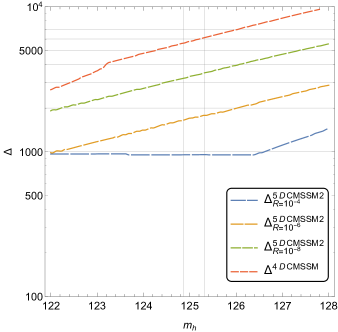
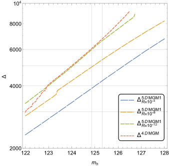
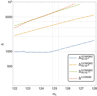
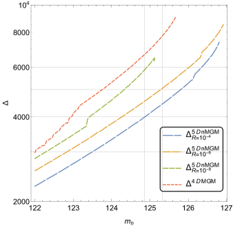
| CMSSM | |||||||
|---|---|---|---|---|---|---|---|
| Model: | 1 | 2 | |||||
| R: | |||||||
| 3.14 | 3.45 | 3.84 | 1.76 | 2.40 | 3.23 | 4.58 | |
| 2.44 | 2.82 | 3.1 | 0.75 | 1.1 | 2.2 | 3.59 | |
| 0.85 | 1.02 | 1.23 | 0.21 | 0.38 | 0.81 | 1.26 | |
| 1.82 | 2.20 | 2.50 | 2.1 | 2.3 | 2.4 | 2.77 | |
| MGM | |||||||
| Model: | 1 | 2 | |||||
| R: | |||||||
| 3.12 | 3.45 | 3.84 | 1.76 | 2.40 | 3.23 | 4.59 | |
| 2.57 | 2.77 | 3.18 | 0.81 | 1.47 | 2.2 | 3.92 | |
| 0.80 | 0.91 | 1.08 | 0.17 | 0.37 | 0.81 | 1.32 | |
| 1.82 | 2.20 | 2.44 | 1.43 | 1.8 | 1.90 | 2.31 | |
| nMGM | ||||
|---|---|---|---|---|
| Model: | 1 | |||
| R: | ||||
| 3.81 | 4.41 | 5.69 | 6.41 | |
| 2.33 | 2.64 | 3.15 | 3.69 | |
| 0.79 | 0.93 | 1.01 | 1.05 | |
| 1.92 | 2.36 | 2.92 | 3.31 | |
6 Conclusions
In this paper we explored the implementation of the five dimensional renormalisation group equations of a number of supersymmetric extensions of the MSSM, into a full C++ spectrum generator, along with self energy corrections for the Higgs mass.
Our key result is showing that modified five dimensional RGEs can result in spectra very different from the usual case. The is because in 5D the heavy gluino does not necessarily dominate running of other soft terms during power law running, as in our model 2. Thus we can easily obtain maximal stop mixing and much less fine tuned spectra, even with standard sets of soft terms at the SUSY breaking scale. This is also very interesting because in 5D models the least fine tuned spectra with correct Higgs mass can easily predict soft superpartner masses within LHC reach, even for standard patterns of soft terms. Interestingly, this means the most interesting parts of the parameter space can be probed during next run of the LHC, which is not usually the case in 4D models.
We explored models where the 1st and 2nd generation are in the bulk and a model in which the 1st and 2nd generation is on the same brane as the supersymmetry breaking sector and the 3rd generation is located on an opposite brane, resulting in a spectrum of stops lighter than other squarks. Obtaining lighter stop soft terms at the SUSY breaking scale did not result in a more natural spectrum. The reason is non negligible fine-tuning price of heavier first two generations and heavier Higgs sector which give only a subleading correction to the light Higgs mass.
The final advantage is a low scale of unification of gauge couplings and a low supersymmetry breaking scale. And also much better unification of Yukawa couplings (especially in model 2) which gives hope for a very interesting five dimensional UV completion of such models.
Acknowledgements
This work was partially supported by the Foundation for Polish Science International PhD Projects Programme co-financed by the EU European Regional Development Fund and by National Science Centre under research grants DEC-2012/04/A/ST2/00099 and DEC- 2014/13/N/ST2/02712. ML was supported by the Polish National Science Centre under doctoral scholarship number 2015/16/T/ST2/00527.
Appendix A Numerical procedure
In this appendix we outline the implementation of the RG-solver and spectrum generator used in this paper. The numerical procedure we use is similar to the ones used in existing codes Allanach:2001kg ; Porod:2003um ; Djouadi:2002ze . We work with quantities renormalized in and use renormalization group equations (RGE), to iteratively find low energy parameters for a given set of high energy soft terms.
A.1 Scale
At the scale we include radiative corrections to couplings. We set Yukawa couplings using the tree-level relations
| (10) |
where are fermion masses and is the Higgs vev. At the first iteration we use physical masses and SM Higgs vev GeV. During subsequent iterations above quantities are renormalized in scheme and one-loop SUSY corrections are included. To calculate the top mass we use 2-loop QCD corrections Avdeev:1997sz and 1-loop corrections from super-partners from the appendix of Pierce:1996zz . While calculating the bottom mass we follow Les Houches Accord Skands:2003cj , starting from running mass in scheme in SM . Next applying the procedure described in Baer:2002ek we find mass at , from which we get MSSM value by including corrections described in appendix D of Pierce:1996zz . While calculating the tau mass we include only leading corrections approximated in Pierce:1996zz . We calculate the Higgs vev in the MSSM using
| (11) |
where we include self interactions described in appendix D of Pierce:1996zz . To calculate , , in in the MSSM we use the procedure described in appendix C of Pierce:1996zz .
A.2 RGE and scale
After calculating coupling constants at the scale we numerically solve RGEs Martin:1997ns ,Yamada:2001ck , to find their values at the scale , at which we include the soft breaking terms. Then we solve RGEs again to find soft terms, coupling constants, and Higgs vev at the scale . At first iteration we take and and run to the scale at which the above equation is fulfilled.
A.3 Electroweak symmetry breaking
In order to obtain correct electroweak symmetry breaking we use minimization conditions for the scalar potential to find new values of and . We include radiative corrections in these equations by the substitution
| (12) |
We include full one-loop corrections to and presented in appendix E of Pierce:1996zz and leading two-loop corrections Dedes:2002dy ; Dedes:2003km ; Brignole:2002bz ; Brignole:2001jy ; Degrassi:2001yf . Since these corrections depend on sparticle masses which in turn depend on the parameter that we aim to calculate, an iterative calculation is performed to obtain new values of and .
If the new values differ significantly from the ones obtained in previous repetition of the whole algorithm described above, we run back to the scale and repeat the whole calculation once again. If however the values of and converged, we can move on to teh calculation of physical masses.
A.4 Calculation of physical masses
To calculate physical masses we use only leading corrections described in Pierce:1996zz everywhere but the Higgs sector. In the Higgs masses calculation we use full one-loop corrections from Pierce:1996zz and leading two-loop corrections described in Dedes:2002dy ; Dedes:2003km ; Brignole:2002bz ; Brignole:2001jy ; Degrassi:2001yf .
A.5 Fine-tuning
After the calculation of the spectrum is finished, one has a whole set of parameters and couplings that predict correct electroweak symmetry breaking. In order to calculate fine-tuning we solve the RGEs from scale down to with one of the fundamental parameters changed slightly at the high scale . Than at the scale we recalculate the spectrum and use minimization conditions to calculate a new value of and to obtain our new prediction for , which means that we calculate numerically the derivative in the definition of fine-tuning (8). We repeat that procedure for all parameters and obtain our final result as a maximum of results obtained for each of those parameters (as in (9)).
References
- (1) ATLAS Collaboration, G. Aad et al., Observation of a new particle in the search for the Standard Model Higgs boson with the ATLAS detector at the LHC, Phys.Lett. B716 (2012) 1–29, [arXiv:1207.7214].
- (2) CMS Collaboration, S. Chatrchyan et al., Observation of a new boson at a mass of 125 GeV with the CMS experiment at the LHC, Phys.Lett. B716 (2012) 30–61, [arXiv:1207.7235].
- (3) I. Antoniadis, A Possible new dimension at a few TeV, Phys. Lett. B246 (1990) 377–384.
- (4) A. Pomarol and M. Quiros, The Standard model from extra dimensions, Phys. Lett. B438 (1998) 255–260, [hep-ph/9806263].
- (5) A. Abdalgabar, A. S. Cornell, A. Deandrea, and M. McGarrie, Natural Supersymmetry and Unification in Five Dimensions, arXiv:1504.7749.
- (6) A. Abdalgabar, A. S. Cornell, A. Deandrea, and M. McGarrie, Large At Without the Desert, JHEP 1407 (2014) 158, [arXiv:1405.1038].
- (7) Z. Lalak and M. Lewicki, Fine-tuning in GGM and the 126 GeV Higgs particle, JHEP 1305 (2013) 125, [arXiv:1302.6546].
- (8) B. Allanach, SOFTSUSY: a program for calculating supersymmetric spectra, Comput.Phys.Commun. 143 (2002) 305–331, [hep-ph/0104145].
- (9) W. Porod, SPheno, a program for calculating supersymmetric spectra, SUSY particle decays and SUSY particle production at e+ e- colliders, Comput.Phys.Commun. 153 (2003) 275–315, [hep-ph/0301101].
- (10) A. Djouadi, J.-L. Kneur, and G. Moultaka, SuSpect: A Fortran code for the supersymmetric and Higgs particle spectrum in the MSSM, Comput.Phys.Commun. 176 (2007) 426–455, [hep-ph/0211331].
- (11) F. Staub, From Superpotential to Model Files for FeynArts and CalcHep/CompHep, Comput.Phys.Commun. 181 (2010) 1077–1086, [arXiv:0909.2863].
- (12) F. Staub, Automatic Calculation of supersymmetric Renormalization Group Equations and Self Energies, Comput.Phys.Commun. 182 (2011) 808–833, [arXiv:1002.0840].
- (13) F. Staub, SARAH 3.2: Dirac Gauginos, UFO output, and more, Computer Physics Communications 184 (2013) pp. 1792–1809, [arXiv:1207.0906].
- (14) F. Staub, SARAH 4: A tool for (not only SUSY) model builders, Comput.Phys.Commun. 185 (2014) 1773–1790, [arXiv:1309.7223].
- (15) A. Hebecker, 5-D superYang-Mills theory in 4-D superspace, superfield brane operators, and applications to orbifold GUTs, Nucl.Phys. B632 (2002) 101–113, [hep-ph/0112230].
- (16) E. A. Mirabelli and M. E. Peskin, Transmission of supersymmetry breaking from a four-dimensional boundary, Phys.Rev. D58 (1998) 065002, [hep-th/9712214].
- (17) M. McGarrie and R. Russo, General Gauge Mediation in 5D, Phys.Rev. D82 (2010) 035001, [arXiv:1004.3305].
- (18) A. S. Cornell, A. Deandrea, L.-X. Liu, and A. Tarhini, Scaling of the CKM Matrix in the 5D MSSM, Phys.Rev. D85 (2012) 056001, [arXiv:1110.1942].
- (19) M. McGarrie, 5D Maximally Supersymmetric Yang-Mills in 4D Superspace: Applications, JHEP 1304 (2013) 161, [arXiv:1303.4534].
- (20) G. Bhattacharyya and T. S. Ray, A phenomenological study of 5d supersymmetry, JHEP 05 (2010) 040, [arXiv:1003.1276].
- (21) A. Delgado, A. Pomarol, and M. Quiros, Supersymmetry and electroweak breaking from extra dimensions at the TeV scale, Phys.Rev. D60 (1999) 095008, [hep-ph/9812489].
- (22) K. R. Dienes, E. Dudas, and T. Gherghetta, Grand unification at intermediate mass scales through extra dimensions, Nucl. Phys. B537 (1999) 47–108, [hep-ph/9806292].
- (23) D. E. Kaplan, G. D. Kribs, and M. Schmaltz, Supersymmetry breaking through transparent extra dimensions, Phys. Rev. D62 (2000) 035010, [hep-ph/9911293].
- (24) Z. Chacko, M. A. Luty, A. E. Nelson, and E. Ponton, Gaugino mediated supersymmetry breaking, JHEP 01 (2000) 003, [hep-ph/9911323].
- (25) M. McGarrie, Gauge Mediated Supersymmetry Breaking in Five Dimensions, arXiv:1109.6245.
- (26) G. Giudice and R. Rattazzi, Theories with gauge mediated supersymmetry breaking, Phys.Rept. 322 (1999) 419–499, [hep-ph/9801271].
- (27) Particle Data Group Collaboration, K. A. Olive et al., Review of Particle Physics, Chin. Phys. C38 (2014) 090001.
- (28) J. R. Ellis, K. Enqvist, D. V. Nanopoulos, and F. Zwirner, Aspects of the Superunification of Strong, Electroweak and Gravitational Interactions, Nucl.Phys. B276 (1986) 14.
- (29) R. Barbieri and G. Giudice, Upper Bounds on Supersymmetric Particle Masses, Nucl.Phys. B306 (1988) 63.
- (30) P. H. Chankowski, J. R. Ellis, M. Olechowski, and S. Pokorski, Haggling over the fine tuning price of LEP, Nucl.Phys. B544 (1999) 39–63, [hep-ph/9808275].
- (31) L. Avdeev and M. Y. Kalmykov, Pole masses of quarks in dimensional reduction, Nucl.Phys. B502 (1997) 419–435, [hep-ph/9701308].
- (32) D. M. Pierce, J. A. Bagger, K. T. Matchev, and R.-j. Zhang, Precision corrections in the minimal supersymmetric standard model, Nucl.Phys. B491 (1997) 3–67, [hep-ph/9606211].
- (33) P. Z. Skands, B. Allanach, H. Baer, C. Balazs, G. Belanger, et al., SUSY Les Houches accord: Interfacing SUSY spectrum calculators, decay packages, and event generators, JHEP 0407 (2004) 036, [hep-ph/0311123].
- (34) H. Baer, J. Ferrandis, K. Melnikov, and X. Tata, Relating bottom quark mass in DR-BAR and MS-BAR regularization schemes, Phys.Rev. D66 (2002) 074007, [hep-ph/0207126].
- (35) S. P. Martin, A Supersymmetry primer, Adv.Ser.Direct.High Energy Phys. 21 (2010) 1–153, [hep-ph/9709356].
- (36) Y. Yamada, Two loop renormalization of tan beta and its gauge dependence, Phys.Lett. B530 (2002) 174–178, [hep-ph/0112251].
- (37) A. Dedes and P. Slavich, Two loop corrections to radiative electroweak symmetry breaking in the MSSM, Nucl.Phys. B657 (2003) 333–354, [hep-ph/0212132].
- (38) A. Dedes, G. Degrassi, and P. Slavich, On the two loop Yukawa corrections to the MSSM Higgs boson masses at large tan beta, Nucl.Phys. B672 (2003) 144–162, [hep-ph/0305127].
- (39) A. Brignole, G. Degrassi, P. Slavich, and F. Zwirner, On the two loop sbottom corrections to the neutral Higgs boson masses in the MSSM, Nucl.Phys. B643 (2002) 79–92, [hep-ph/0206101].
- (40) A. Brignole, G. Degrassi, P. Slavich, and F. Zwirner, On the O(alpha(t)**2) two loop corrections to the neutral Higgs boson masses in the MSSM, Nucl.Phys. B631 (2002) 195–218, [hep-ph/0112177].
- (41) G. Degrassi, P. Slavich, and F. Zwirner, On the neutral Higgs boson masses in the MSSM for arbitrary stop mixing, Nucl.Phys. B611 (2001) 403–422, [hep-ph/0105096].