The forward approximation as a mean field approximation for the Anderson and Many Body Localization transitions
Abstract
In this paper we analyze the predictions of the forward approximation in some models which exhibit an Anderson (single-) or many-body localized phase. This approximation, which consists in summing over the amplitudes of only the shortest paths in the locator expansion, is known to over-estimate the critical value of the disorder which determines the onset of the localized phase. Nevertheless, the results provided by the approximation become more and more accurate as the local coordination (dimensionality) of the graph, defined by the hopping matrix, is made larger. In this sense, the forward approximation can be regarded as a mean field theory for the Anderson transition in infinite dimensions. The sum can be efficiently computed using transfer matrix techniques, and the results are compared with the most precise exact diagonalization results available.
For the Anderson problem, we find a critical value of the disorder which is off the most precise available numerical value already in 5 spatial dimensions, while for the many-body localized phase of the Heisenberg model with random fields the critical disorder is strikingly close to the most recent results obtained by exact diagonalization. In both cases we obtain a critical exponent . In the Anderson case, the latter does not show dependence on the dimensionality, as it is common within mean field approximations.
We discuss the relevance of the correlations between the shortest paths for both the single- and many-body problems, and comment on the connections of our results with the problem of directed polymers in random medium.
I Introduction
The propagation of waves and quantum particles in a disordered medium is a fascinating and challenging problem in statistical mechanics, with plenty of relevance for experiments Abrahams (2010); Billy et al. (2008); Roati et al. (2008). Among the phenomena that occur in such a setting, Anderson localization is probably the most striking Anderson (1958); Abrahams (2010). “Anderson’s theorem” in Ref. Anderson, 1958 states that for sufficiently strong disorder, diffusive transport is completely suppressed in single particle problems on a lattice. The study of the transition that separates the two phases (localized and delocalized) has resisted an exact solution for about 60 years, and numerical methods are still at the core of the advances in this topic Evers and Mirlin (2008).
Recently, interest in Anderson localization has surged due to the work by Basko, Aleiner and Altshuler Basko et al. (2006), henceforth denoted by BAA. There, the phenomenon of many-body localization (MBL), i.e. the stability of the Anderson insulator to the addition of interactions, is investigated. BAA’s work has been extended and re-interpreted in several other works Oganesyan and Huse (2007); Pal and Huse (2010); De Luca and Scardicchio (2013); Serbyn et al. (2013); Imbrie (2014); Kjäll et al. (2014); Huse et al. (2014); Laumann et al. (2014); Chandran et al. (2015); Ros et al. (2015); Luitz et al. (2015), and MBL appears now to be the most robust mechanism to break the ergodicity that is typical of generic interacting systems.
The core of BAA’s analysis relies on perturbatively accounting for the interactions, at finite temperature and particle density. Technically, they consider the perturbation theory for the imaginary part of the propagator of an excitation on top of an eigenstate by means of the Keldysh formalism. For sufficiently weak interactions, the perturbative series is shown to converge with probability equal to one. In the spirit of Ref. Anderson, 1958 this implies the localization of the excitations themselves, and the absence of transport.
As an alternative route, the MBL problem can be interpreted as a single particle tight-binding problem in the space of many-body configurationsAltshuler et al. (1997), with the interactions playing the role of an effective hopping. However, several issues arise in this formulation. First, the on-site energies in the resulting effective lattice are not independent variables drawn from the same distribution, but they are strongly correlated. Secondly, the connectivity of a configuration in the many-body problem scales with (a power of) the system size: it diverges in the thermodynamic limit, and thus it is impossible to define a limiting graph. As a consequence, one needs to define an effective connectivity which stays of in the thermodynamic limit (a similar phenomenon is observed in Ref. Huse et al., 2015). Finally, the number of paths of a given length connecting two many-body configurations grows factorially with the distance between them, the distance being defined as the minimum number of actions of the interaction operator needed to connect the initial to the final configuration. Since the distance between two configurations can be of the order of the system size, the number of paths can grow factorially in the system size. When the mapping to a single particle problem is applied to a system of interacting spins, it results into a correlated-disorder problem on a (section of) an -dimensional hypercube.
Despite these complications, in some recent works Laumann et al. (2014); Ros et al. (2015); Huse et al. (2015) this approach has been used successfully to estimate, among other things, the boundaries of the MBL region. The analytical calculations in Refs. Laumann et al., 2014; Huse et al., 2015 were shown to be in very good agreement with the numerical results in the same papers, obtained with exact diagonalization. The analytic results are derived revisiting an approximation already used in Refs. Anderson, 1958; Abou-Chacra et al., 1973; Medina and Kardar, 1992; Altshuler et al., 1997, which consists in calculating the Green’s functions by retaining only the lowest order in the hopping. Recently, this approximation has been used in Ref. De Luca et al., 2014 to derive the power-law tail of the distribution of the wave function amplitudes on a Bethe lattice in the localized phase.
In this paper we discuss in detail this approximation, dubbed “forward approximation” (FA), by illustrating its virtues and limitations and its connections to other, seemingly unrelated, problems of statistical physics. The paper is organized as follows: in Section II we derive the expression for the wave function amplitudes in forward approximation, and discuss a criterion for localization given in terms of the probability of resonances. In Section III, after recalling some known results on the Anderson model on the Bethe lattice, we focus on -dimensional systems (with ). We compare the analytic results we get for the critical disorder within the FA with the numerics, showing how the approximation gives better results as the dimensionality is increased. We then discuss the application of the aforementioned technique to a many-body problem of interacting spins in a disordered environment. In Section IV we discuss the relevance of the correlations and interference between different paths connecting two configurations, both for the single particle and for the many body problem. In the Conclusions we comment on the various possible directions in which this work can be extended, focusing in particular on the application of the forward approximation to the study of the MBL phase and of the many-body localization-delocalization transition.
II Derivation
II.1 The forward approximation for the eigenfunctions
To begin with, we derive the expression for the wave function amplitudes in FA for a single particle hopping on a finite lattice with on-site disorder. We consider the Hamiltonian:
| (1) |
In the Anderson model, the are independent random variables uniformly distributed in , one for each of the sites in the lattice. The edges define the lattice geometry. The lattice constant is set to one, and we denote with the length scale characterizing the size of the lattice (for a cubic lattice in dimension the diameter is , for a Bethe lattice or regular random graph it is , where is the connectivity of the lattice). The distance between two arbitrary sites of the lattice is the number of edges in a shortest path connecting them. We refer to it as the lattice distance in the following.
We consider the matrix elements of the resolvent between two states associated to the sites in the lattice:
| (2) |
at energy . They have the following expansion in series of
| (3) |
where the sum runs over all the paths in the lattice connecting the sites and , and labels the sites visited by the path (site excluded). Given two sites at lattice distance , the lowest orders in the expansion are
| (4) |
where the sites belong to one of the shortest paths connecting and .
On the other hand, from the spectral decomposition it follows
| (5) |
and thus the residue at gives
| (6) |
assuming no degeneracy of the eigenvalues.
The path representation (3) does not have a pole at , to no order in . To get the exact poles it is necessary to re-sum the closed paths in the series expansion. Once this is done, the full series is re-cast into a sum over the non-repeating paths connecting the sites and :
| (7) |
Here is the local self-energy at the site , defined through the identity:
| (8) |
It is equal to the sum of the amplitudes of all the closed paths in which site appears only as starting and ending point; to lowest order in
| (9) |
where is the set of nearest neighboring sites of . The path-dependent term is a modified self-energy, which re-sums the loops around site , never crossing site again, nor any of the sites already visited by the non-repeating path .
The expansion (7) in non-repeating paths has several advantages. First, while is an infinite set, even for a finite lattice, is finite for a finite lattice. Moreover, (7) is free of the divergences affecting (3) that are due to local resonances, i.e. to sites at bounded distance satisfying with small (we clarify the exact meaning of small in Sec. II.2). Local resonances necessarily occur also in the localized phase, and produce arbitrarily large factors in (3), corresponding to the paths repeatedly hitting the resonant sites an arbitrary number of times. These repetitions of large factors lead to the divergence of the naive perturbation series in , but are re-summed into self energy corrections in (7). The “renormalized” expansion in non-repeating paths is found to converge in the localized phase Anderson (1958), when resonances do not proliferate at asymptotically large distances in space, and the hopping hybridizes only the degrees of freedom in a finite, albeit possibly big, region of space. An analogous resummation procedure is discussed in Ref. Ros et al., 2015, where the perturbation theory for quasi-local conserved operators is shown to converge in the MBL phase.
The expression for the eigenfunction is obtained from the resolvent as follows: the eigenenergy satisfies , thus the first factor of (7) has a pole at with residue , as it follows from (8) and (6). Then:
| (10) |
which gives
| (11) |
with obtained from using (6).111A similar argument gives a perturbative series in for the conductance.
From (11) we can read the expression of the wave function amplitudes to lowest order in . Assume that labels an eigenstate localized at site for . Since , we have to lowest order , , , giving
| (12) |
where the set contains the shortest paths from to . Note that this derivation does not rely on the particular structure of the lattice nor on the independence of the on-site energies, and thus it can be straightforwardly generalized to hopping problems on graphs with different geometry or more general distribution of the random energies, such as the ones in Sec. III.3.
The effect of the modified self energy corrections is to weaken the role of resonances. Indeed, let us assume that in the path there is a site which is resonant with , . In this case the forward approximation (12) will contain the very large term . However, the correction in the previous site also contains such large term, leading to a compensation. As we shall see in the following, neglecting this effect leads to an overestimate of the minimum disorder strength needed to localize the system. On the other hand, the loops contributing to the self energy corrections become less relevant when the dimensionality (or connectivity) of the lattice is increased. Thus, the FA is expected to give faithful results in higher dimension (see Sec. III.2).
II.2 Probability of resonances and criterion for localization
For a single particle problem on a finite dimensional lattice, we define an eigenstate of a system of size localized if (with probability 1 over the disorder realizations) the probability of finding a particle at a distance from the localization center of the state tends to zero in the limit of large . More precisely, let denote the localization center of , and
| (13) |
We define the state localized if there exists a finite such that
| (14) |
Namely, we require that the random numbers can be enclosed in an exponential envelope for all sufficiently far from the localization center of the state. By means of the Kubo formula, it is possible to show that this condition on the eigenstates implies the vanishing of the DC conductivity. We identify the localization length of with the minimum value of for which Eq. (14) is true. It does, in general, depend on the state; however, it is supposed to depend smoothly on the energy in the thermodynamic limit. A mobility edge exists whenever there is band of energies for which such minimum is not finite. In particular, at fixed energy and at the corresponding critical value of disorder , the localization length diverges and the asymptotic bound in Eq. (14) ceases to hold for any finite . This entails that for any arbitrarily small, positive and at arbitrarily large distances from the localization center, there exist sites such that the ratio exceeds the constant with some finite probability. We expect the delocalized phase to be characterized by the stronger condition:
| (15) |
holding for any arbitrarily small, strictly positive value of .
From the equations (14), (15) it follows that the localization-delocalization transition can be detected analyzing the statistics of the wave function amplitudes as a function of distance. In the following, we compute the wave function amplitudes in FA and determine numerically the probability in Eq.(15), choosing of the order of the numerical precision. We refer to the resulting probability as the “probability of resonances”. The terminology is motivated by the fact that within the FA, an amplitude of at a site at distance from the localization center corresponds to a resonance between the two sites. Indeed, the corresponding two sites problem can be considered as a two-level system with reduced Hamiltonian
| (16) |
where , and
| (17) |
where the products are taken over all sites in the path, excluding . The sites are resonant when the energy difference is small, and precisely . Considering to lowest order in , one finds that this is equivalent to , with computed in the lowest order FA. Thus, with (14) and (15) one is probing the statistics of resonances within the FA, and requiring that the probability to find at least a resonant site at any sufficiently large distance from the localization center decays to zero in the localized phase. This criterion involving resonances allows to obtain an estimate for the critical disorder within the FA also on the Bethe lattice, where the exact eigenstates satisfy Eq. (14) even in the delocalized phase, due to normalization.
III Results
III.1 Warming up: the Bethe lattice
The simplest setting for the application of the forward approximation is a Bethe lattice: in this case, given two sites , there is only one non-repeating path connecting them, along which all the energies are i.i.d. . This makes the problem amenable to analytic calculations.Abou-Chacra et al. (1973); Abou-Chacra and Thouless (1974); Altshuler et al. (1997) We briefly recall some results in the following.
Let be the root of the tree, and the branching number (the connectivity is ). Within the FA we get that the wave function at one particular point at distance from the root is given by
| (18) |
This random variable has a power-law tail distribution for any distribution of having a support such that , as one can see from the divergence of the first moment of the absolute value of . It is convenient to consider the distribution of the logarithm of , whose moments are all finite. Let us remind the reader that we choose , and in this calculation for simplicity we set . Defining
| (19) |
we find that
| (20) |
The ratio is the typical decay of wave function amplitudes from the origin of localization
| (21) |
However, this is not the localization length as defined in (14). The latter is indeed a uniform bound over the full set of points at distance from the localization center: it is determined by the decay rate of the maximal amplitude over sites in each shell at distance . This is a point-to-set correlation function decay, which is familiar in the study of disordered systems on the Bethe lattice (on a regular lattice the point-to-set is substituted by the point-to-point, but with exponentially many shortest paths leading to the final point).
The typical value of the maximal amplitude among samplings is the largest solution of
| (22) |
Here is the distribution of , and the paths are treated as independent. For large , what matters is the tail of the distribution . If we rescale
| (23) |
we get, for large :
| (24) |
The probability distribution of can be found inverting its Laplace transform, which is computable since is a sum of i.i.d. variables. The maximum over samplings of is the solution of
| (25) |
and . Localization occurs as long as , so the critical condition can be written as
| (26) | |||||
| (27) |
By eliminating we recover the familiar Abou-Chacra et al. (1973) equation:
| (28) |
Moreover, is given in terms of as
| (29) |
so we can write the localization length as
| (30) |
This gives a mean-field exponent for the divergence of the localization length at the transition:
| (31) |
Note that irrespective of the value of the disorder. The belief expressed in Ref. De Luca et al., 2014 is that this behavior persists even within the delocalized regime, in the form of very irregular (multi fractal) eigenstates. Note additionally that the difference between and is due to the exponential sampling of the probability distribution, and it extends both to the finite-dimensional cube and to the many-body case.
III.2 d-dimensional cube
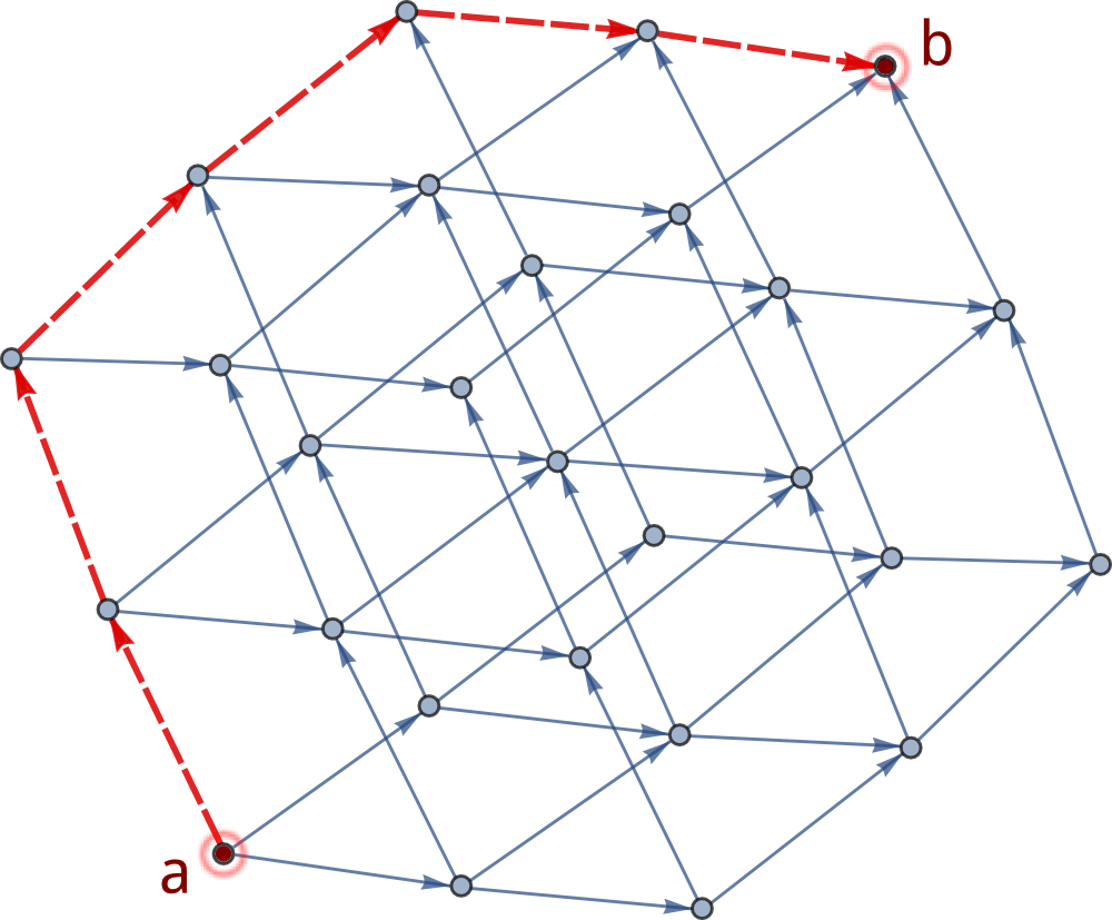
Consider now the case of a -dimensional lattice of side , and let be the site at one corner of the cube, which we treat as the origin. Given any other site , the orientation of the non-repeating, shortest paths from to induces a natural orientation of the edges of the cube, which is thus directed, see Fig. 1. Let be the lattice distance of the sites with respect to the origin : for a cube of side , the maximum is , corresponding to the site at the opposite corner of the cube with respect to .
In an infinite cube the number of points at distance from the origin is , and thus it grows at most polynomially in , slower than . Naively, one would be led to think that the transition is given by the divergence of , see Eq. (21). However, the number of minimum length paths leading from the origin to an arbitrary site at lattice distance scales exponentially with , as . Therefore, unlike in the Bethe lattice case, in finite dimension the wave function amplitude at a given site is a sum over exponentially many correlated terms
| (32) |
where
| (33) |
and the random variables are uniformly distributed in . In the following, we consider the probability distribution of the random variable
| (34) |
for different values of . Here denotes the maximum among all the rescaled amplitudes (33) at sites that are at lattice distance with respect to the origin . The probability of resonances for arbitrary values of and , see Eq. (15), is easily recovered from the cumulative distribution function of as:
| (35) |
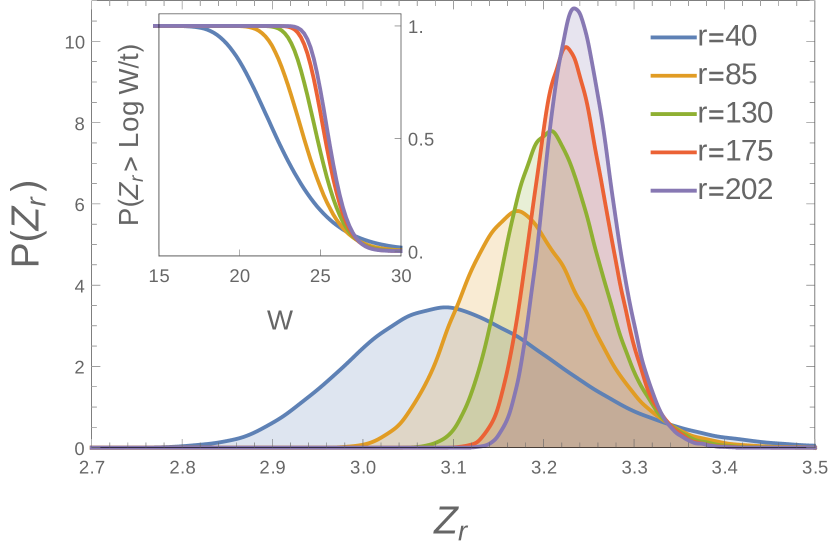
with arbitrarily close to zero. According to Eqs. (14) and (15), the density of becomes asymptotically peaked at for , with width going to zero with . Thus, the critical value of disorder can be estimated inspecting the scaling with of the probability density of .
The distribution of is hard to determine analytically, due to the correlation between the different shortest paths. To account for such correlations, we compute the amplitude (33) numerically by means of a transfer matrix technique, and use the resulting values to determine the probability (35) with smaller than the numerical precision. The convenience of the transfer matrix method relies on the fact that it takes only polynomial time in , as it was realized by Medina and KardarMedina and Kardar (1992) in their treatment of the Nguyen, Spivak, and Shklovskii Nguyen et al. (1985a); *nguyen1985jetp2; *nguyen1986hopping (NSS) model. 222Note that the present calculation does not reduce to the one for the NSS case, since a major difference between the two models is in the statistics of energy denominators: in the NSS model the binary disorder (with probability or ) does not allow for resonances due to a single site. Rather, the resonances arise from contributions of different paths. This led to a body of work following Ref. Medina and Kardar, 1992, on the presence of a sign transition, where effects from different paths accumulate in order to break the sign symmetry. In the FA for the Anderson case, the energy denominators can be arbitrarily small with finite probability, generating path weights that are fat tailed distributed. The fat tail of this distribution is crucial for the considerations below.
The numerical computation is as follows. We fix and introduce the matrix defined as
| (36) |
where is the forward adjacency matrix of the lattice (that is, the adjacency matrix associated to the directed cube of Fig.1), and is a diagonal matrix with components:
| (37) |
We initialize the system in the state completely localized in the origin , and iteratively apply the transfer matrix . A single iteration gives
| (38) |
where are the forward neighbors of site . The value of equals , where is the state completely localized in the site and is the lattice distance between and .
We fix and compute the rescaled amplitude (33) for all the points on a shell at the same lattice distance from the origin of a hypercube of side . Here is fixed so as to have about points per each size of the hypercube. We determine the maximal among the wave function amplitudes on those sites. We repeat the procedure for hypercubes of different sizes, with disorder realizations for most system sizes, decreasing to realizations only for the biggest system sizes that we consider (e.g. in we take system sizes through , with disorder realizations up to and realizations up to ).
As we discuss in Section IV, the main contribution to the transfer matrix result comes from only one of the exponentially many paths in (33), and the results obtained with the transfer matrix technique are faithfully reproduced by analyzing the statistics of the dominant path alone. The latter can be determined (see Section IV) with an algorithm that is computationally more efficient than the transfer matrix, allowing to access to much bigger system sizes. The results presented in this sections for , as well as for the higher values of in , are obtained with this procedure.
III.2.1 Fluctuations of the wave function amplitudes
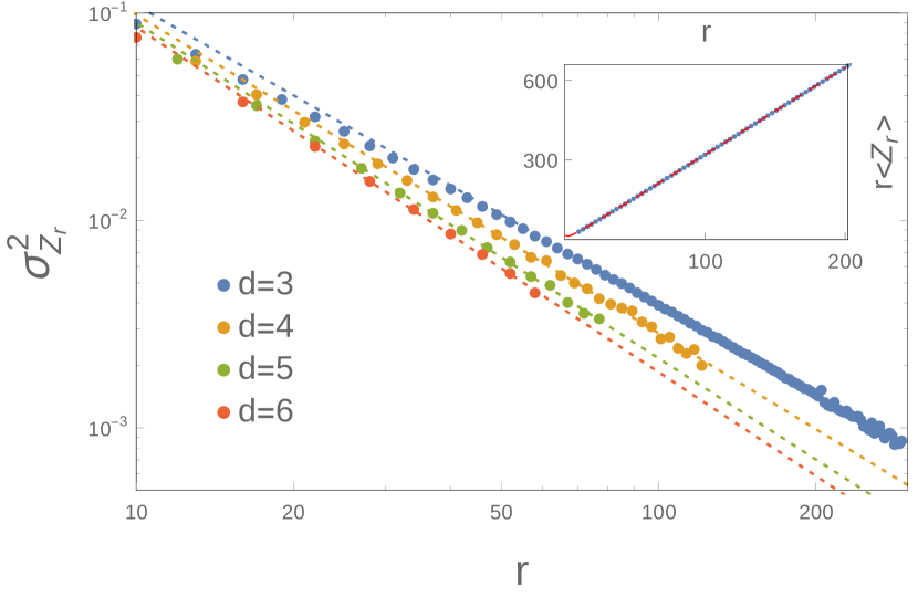
In Fig. 2 we plot the probability density of the variable defined in Eq. (34), for different values of in . The plot shows a drift of the position of the peaks with increasing , together with the shrinking of the width of the distribution, in agreement with the conditions (14), (15). Plots of the -dependence of the variance of (34) are given in Fig. 3, in log-log scale for . The linear behavior indicates that the fluctuations of decay to zero as a power law in , with a coefficient that depends on the dimensionality. The higher cumulants of the distribution exhibit a similar linear behavior in log-log scale. Moreover, the numerical computation indicates that for fixed the probability densities of the variable
| (39) |
collapse to a limiting curve for increasing , see Fig. 4. As shown in the same plot, for fixed and varying dimensionality, the distribution of does not change significantly, except for a weak -dependence of the tails.
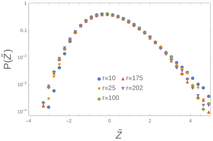
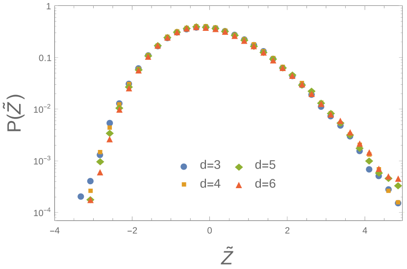
These numerical observations are compatible with the following large scaling form for :
| (40) |
where is a random variable of with a distribution which depends weakly on the dimensionality.
| d=D+1 | ||
|---|---|---|
| 3 | ||
| 4 | ||
| 5 | ||
| 6 |
According to (40), for large the fluctuations decay to zero with the power . From the linear fit of we extract the numerical estimate of the exponent in (40), which we denote with . The results are reported in Table 1.
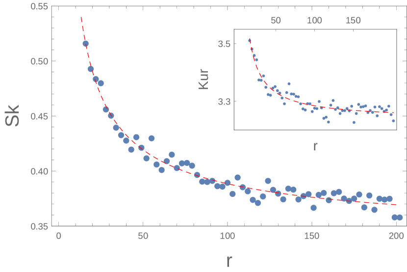
In order to characterize the limiting distribution in Fig. 4, we compute the skewness and the kurtosis of the density of (here denotes the -th cumulant of the distribution). From (40) it follows that these parameters approach the ones corresponding to the variable in the limit of large . We restrict to , for which we have the largest statistics available. Plots of the -dependence of Sk and Kur are given in Fig. 5. The asymptotic values are estimated to be and , see the caption of Fig. 5 for details.
III.2.2 Estimate of the critical disorder
To determine the critical value of disorder for , we extrapolate the asymptotic limit of the typical value of . Since the distribution is not fat tailed, we can equivalently consider the averages of and set:
| (41) |
The inset in Fig. 3 shows the scaling with of . The average grows linearly in , in agreement with Eq. (40). We fit the data with the form
| (42) |
with the numerical values reported in Table 1,.
The resulting estimates of the critical disorder, which we denote with , are displayed in Table 2. For the smallest dimensions, a comparison is made with the critical values determined in Refs. Slevin and Ohtsuki, 2014; Ueoka and Slevin, 2014 by means of a combination of exact diagonalization and transfer matrix techniques.
| d | Error | ||
|---|---|---|---|
| 3 | 39% | ||
| 4 | 16% | ||
| 5 | 0.9% | ||
| 6 | - | - | |
| 7 | - | - |
The data in Table 2 clearly show that the FA gives an upper bound to the critical disorder, since the renormalization of the energy denominators provided by the (modified) self-energy corrections are neglected, and the effects of resonances are thus enhanced. However, increasing the dimensionality the discrepancy between the numerical estimates of decreases; the enhanced precision of the FA result is due to the fact that the loops giving rise to the self-energy corrections become less relevant in higher dimensional lattices, and thus the FA becomes asymptotically exact in this limit.
III.2.3 Divergent length scales and critical exponents
For fixed values of and for finite , the probability of resonances (35) is determined by the tails of the distribution of .
For increasing , the asymptotic limit is approached in a different way at the two sides of the transition: for , the probability of resonances goes to zero exponentially with . Below the transition, the probability converges to one much faster, with corrections that are only double exponential in . We justify analytically this behavior in Appendix A, by computing an approximate expression for the density of the variable . The approximation consists in considering the different paths contributing to it as independent variables.
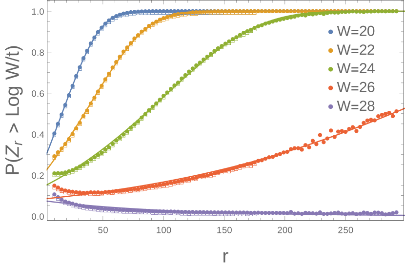
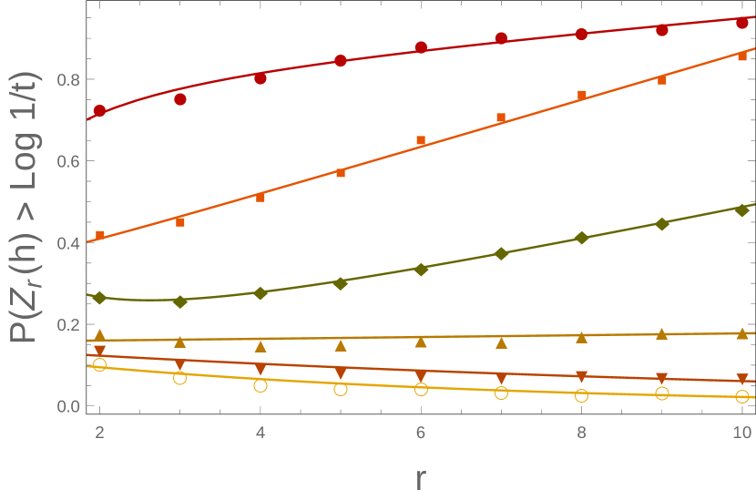
Examples of the fits of the probability of resonances are shown in Fig. 6. To extract a -dependent length scale , we perform an exponential fit of the form:
| (43) |
for . For we determine by means of the linear fit
| (44) |
The length scale is plotted in Fig. 7 for . We expect it to diverge in the same way as the localization length/correlation length does in the localized/delocalized phase, respectively. We find that diverges as a power-law at a critical disorder compatible with the values of listed in Table 2. A fit of the form results in an exponent that is compatible with for all dimensions, consistently with the Bethe lattice picture and with the results in Appendix A. However, some deviations can be observed: a more careful analysis of the numerical data will be presented in a future publication.
III.2.4 Connections with the problem of directed polymers in random medium
In the single particle case, the energy denominators associated to different sites along the paths are independent variables. Thus, the expression for the wave function amplitude in FA, Eq. (12), resembles the expression for the partition function of a directed polymer (DP) in a random potentialDerrida (1990); Derrida and Spohn (1988); Halpin-Healy and Zhang (1995), with the thermal weights for the polymer configurations given by the amplitudes of the different paths. This analogy is not straightforward, due to the occurrence of negative contributions in (12). Nevertheless, it has been fruitfully exploited both for the single particle problem Somoza et al. (2007); Prior et al. (2009); Somoza et al. (2015); Monthus and Garel (2009), and for problems of interacting spins on the Bethe lattice Feigel’man et al. (2010); Ioffe and Mézard (2010); Müller (2013); Yu and Müller (2013).
Motivated by this analogy ,the authors of Ref. Prior et al., 2009 have proposed a scaling form analogous to (40) for the logarithm of the conductance of an Anderson model. There, the conductance in is obtained from the Green functions, which are computed numerically within a modified FA, the modification consisting in taking energy denominators that are not arbitrarily small but are bounded from below. 333Note that if this constraint is relaxed and the energy denominators are allowed to be arbitrarily small, is found to be proportional to the quantity that we are considering. It is shown that the fluctuations of scale with an exponent , and that the distribution of the variable is compatible with a Tracy-Widom distribution.
These results are consistent with the conjectureMedina et al. (1989); Medina and Kardar (1992) that in the strongly localized phase, where the expansion in non-repeating paths is best controlled, the Anderson model in dimension belongs to the same universality class of the directed polymer in dimension , with . In particular, the conjecture implies that in the limit of large the distribution of has the scaling form (40), with coinciding with the droplet exponentFisher and Huse (1991) in dimensions (which is exactly knownHuse et al. (1985) to be equal to for ), and having the same distribution of the fluctuations of the free energy in the disordered phase of the polymer (distributed according to the Tracy-Widom distributionJohansson (2000); Prähofer and Spohn (2000); *prahofer2002scale; *prahofer2004exact in ).
The values of the scaling exponents extracted from our data do not compare well with the droplet exponents of the DP, see Table 1. Curiously, they compare within errors with . We do not have an explanation for this curious behavior, and we leave its analysis for future work. Broadly speaking, the discrepancies with respect to the directed polymer results are generated by the fat-tail of the distribution of the paths amplitudes in (32), produced by the arbitrarily small energy denominators. It might be that the finite size effect are more pronounced in the case of unbounded denominators. On the other hand, it is quite natural to expect that the models of non-repeating paths with bounded amplitude considered in Ref. Prior et al., 2009 exhibit a stronger dependence on the dimensionality, due to the fact that the domination by one single path is less pronounced in that case. We comment more on this point in Sec. IV.
III.3 Heisenberg model with random fields
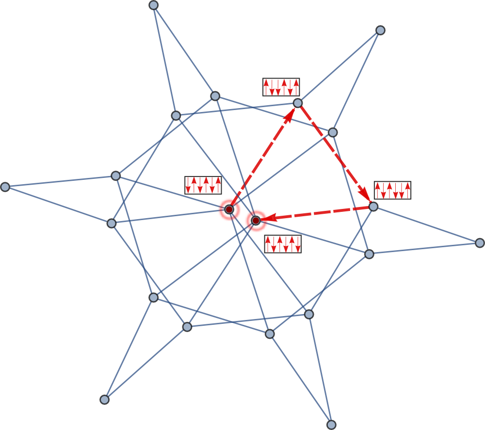
In order to test the forward approximation on a many-body problem, we consider an XXZ spin-1/2 chain in random magnetic field,
| (45) |
where periodic boundary conditions are assumed (), and the random fields are uniformly distributed in . This spin Hamiltonian (45) has been studied in a large number of works Pal and Huse (2010); Žnidarič et al. (2008); Bardarson et al. (2012); De Luca and Scardicchio (2013); Bauer and Nayak (2013); Nanduri et al. (2014); Bar Lev et al. (2015); Mondragon-Shem et al. ; Goold et al. (2015), in which numerical evidence of the existence of a localization-delocalization transition is provided, mainly based on exact diagonalization results. The critical disorder is estimated Luitz et al. (2015) to be for states in the middle of the energy band and parameters and .
As mentioned in the Introduction, the many body problem can be seen as a single particle hopping problem in the “configuration space”. The latter is composed of the product states in the basis of , which span the full Hilbert space and diagonalize . We denote these basis states with , and refer to them as the “computational basis”. The mapping to an hopping problem is obtained by interpreting each state as a vertex of a graph, with associated random energy defined by . The third term in (45) provides the hopping between different sites, thus defining the geometry of the graph. Note that due to spin conservation, the full configuration space, and consequently the graph, are partitioned into disjoint sectors corresponding to different total spin; we restrict to the sector of total spin equal to zero, corresponding to a connected graph with vertices. See Fig. 8 for a pictorial representation of the graph for .
The effective hopping problem can be analyzed using the procedure set up in Sec. II.1: the amplitude of an eigenstate of the effective single particle problem is given in forward approximation by:
| (46) |
where it is assumed that the eigenstate satisfies for .
In the many body language, Eq.(46) provides the expression of the coefficients of the eigenstates of (45) in the computational basis, to lowest order in the coupling . The exponential decay of the coefficients implies localization in the configuration space, meaning that the full many-body eigenstates are effectively a superposition of product states which differ only by configurations distant from the initial configuration. The two main consequences of this structure of the wave function is that they have significantly less entanglement than ergodic states Buccheri et al. (2011); De Luca and Scardicchio (2013); Bauer and Nayak (2013) and that, using Kubo’s formula for linear response Ros et al. (2015), one can prove that they cannot support transport on macroscopic distances.
Similarly to the Anderson case, we fix an initial configuration of spins and we look at the amplitude in perturbation theory on the most distant, fully flipped configuration. In particular, we fix the localization center to be the site correspondent to the Neel state , and consider the wave function amplitude on the site corresponding to the fully flipped Neel state . These two sites are connected by paths on the graph, of length each.
By means of the transfer matrix we compute the rescaled amplitude
| (47) |
for different disorder strength , with given by (46). We consider spin chains of size with hopping and interaction constants respectively and , and . Note that, despite the general framework is the same as in the Anderson problem, the transfer matrix calculation is by no means identical; indeed, in the many body case the energies associated to the different graph vertices are a linear combination of the independent random fields, and are thus correlated. Moreover, the number of paths connecting two sites proliferates with the size of the chain , with a scaling that is faster than exponential. These paths present correlations that are much stronger with respect to the Anderson problem, as we shall discuss in more detail in Sec. IV.
III.3.1 Distribution of the wave function amplitudes and critical disorder
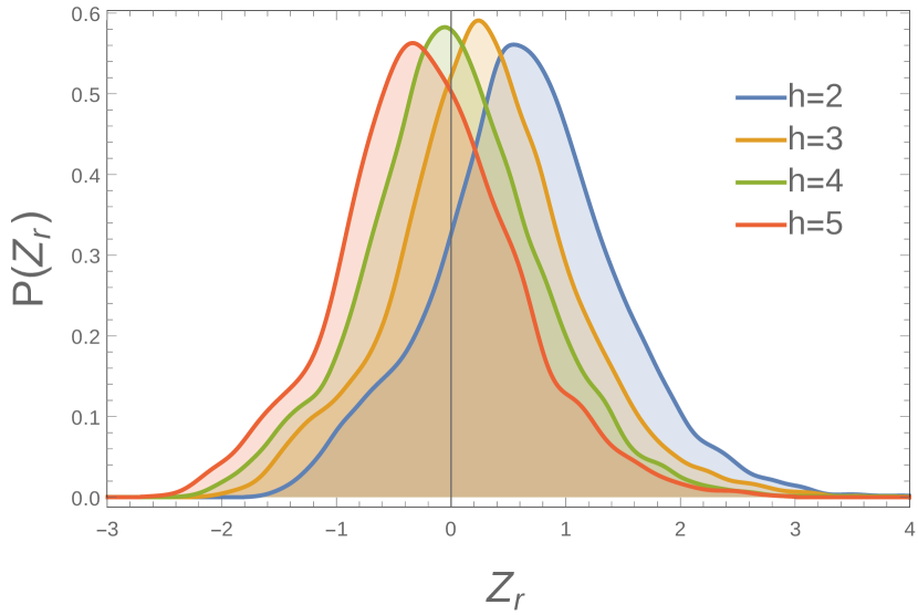
In Fig. 9 we show the probability density of for a chain of length and different values of . Since in the many body case it is not possible to simplify the dependence on the disorder strength , the criterion for the transition reads
| (48) |
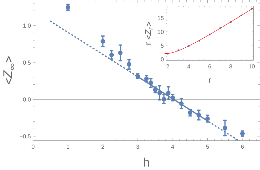
where is the extrapolated value of the average of (47) for fixed . Plots of are given in Fig. 10. Here is extrapolated from the finite size values using the fitting function
| (49) |
For , the critical point is estimated from the condition . The resulting value is , which is, as expected, larger than the result derived with exact diagonalization. Notice also that the corrections are consistent with the intuition that the is the correct mean-field scaling for MBL.
As we discuss in Sec. IV, in the many body case the sum (46) is no longer dominated by a single path. Thus, the algorithm for the best path is not applicable in this context, and the limited system sizes accessible with the transfer matrix do not allow to investigate whether a scaling form exists also for (47) in the limit of large . For the available system sizes, the distributions of the rescaled variables do not seem to collapse to a unique curve, and the scaling of the variances with appears to be compatible with a power-law, but with exponent depending on the disorder strength . However, a more refined numerical analysis is necessary to draw a conclusion on the asymptotic behavior.
III.3.2 Divergent length scales and critical exponents
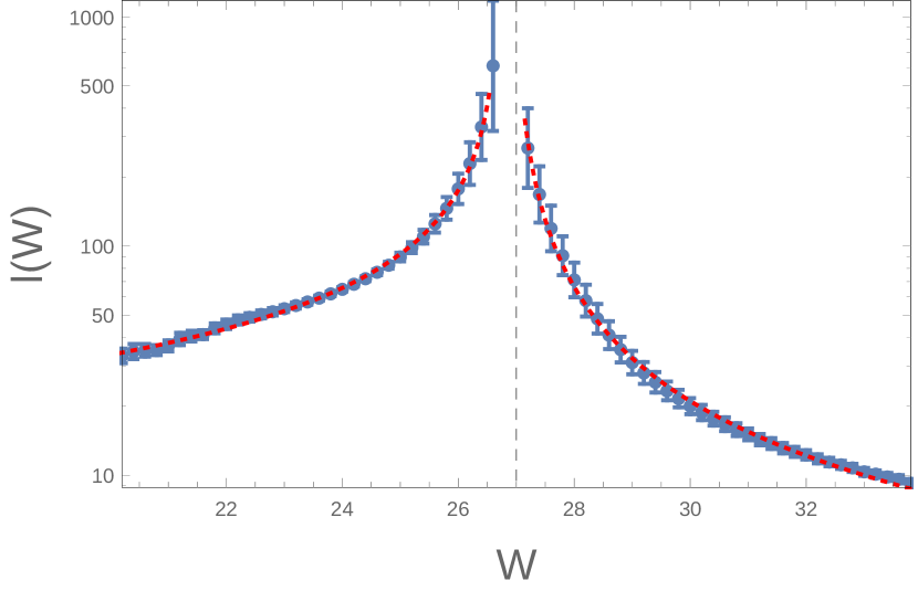
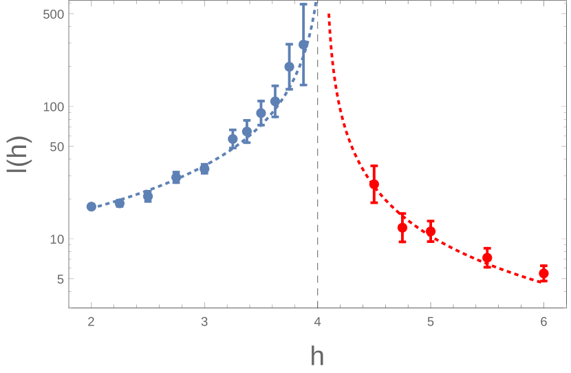
Fig. 11 shows the behavior of the probability of resonances as function of the distance between the Neel states. As expected, the -dependence changes with the disorder: the probability decays to zero at large , and increases towards one for the smaller . We expect the convergence to be exponential in on both sides of the transition; however, the exponential behavior is not clearly detectable in the delocalized phase, due to the few accessible system sizes. For we extract a length scale by fitting the curves in Fig. 11 with the function:
| (50) |
In the localized phase we perform instead the exponential fit:
| (51) |
The length scales extracted with this procedure are shown in Fig. 12, together with the power law fit . The fit is performed separately for and , resulting in an exponent close to in both cases (see Fig. 12 for details). Note the asymmetry of the curve with respect to , which indicates that at fixed the typical distance to find a resonance in the delocalized phase is larger than the localization length at the corresponding value of disorder in the localized phase. A possible consequence of this phenomenon, which occurs also in the Anderson model (see Fig. 7), could be a large “critical region” in the dynamics in the delocalized phase.
IV The structure of the dominating paths
As mentioned in section Sec. III.2, the wave function amplitudes in FA can be interpreted as the partition function for a directed polymer in random medium. However, a relevant difference is that while the weight associated to the polymer is bounded from aboveDerrida and Spohn (1988), the single factors in (33) are unbounded, with diverging average. As a consequence, the strongly localized phase in the Anderson model (where the FA is best controlled) always corresponds to a “frozen” phase of the directed polymer, in which most of the weight in the total sum (12) is given by one single path. An interesting questionBiroli et al. (2012) is whether the freezing phenomenon persists in the delocalized phase in some form, and what this implies that the structure of the eigenstates close to the transition De Luca et al. (2013, 2014).
In this section, we compare the statistics of the wave function amplitudes in FA with that of the optimal path, i.e. the path with maximal amplitude, both for the single particle problem and for the XXZ chain. We show that while in the first case the full sum is strongly dominated by the extremal path amplitude, in the many body case most of the paths have comparable amplitude. However, the much stronger correlation between them gives rise to non-negligible interference effects, resulting in strong cancellations.
IV.1 The single particle case
For the finite dimensional case, we compute the amplitude of the optimal path dominating the sum (12) by means of the Dijkstra algorithm Dijkstra (1959), a graph-search algorithm that determines the path minimizing a given cost function. We consider a directed cube (such as the one in Figure 1) and assign a positive cost to each directed edge :
| (52) |
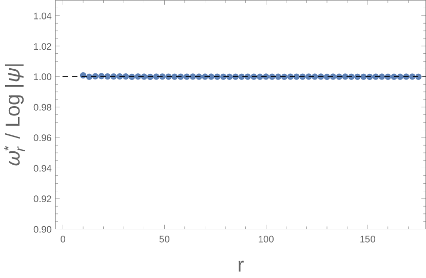
The total cost of a path is the sum of the costs of the edges belonging to it, and the path with maximal amplitude is the one minimizing the total cost function. In order to compare with the transfer matrix results, we compute the ratio between and the full sum (32) computed via the transfer matrix technique, for the same given disorder realization. The distribution of the ratios turns out to be very narrowly peaked around one. Figure 13 displays its average as a function of the length of the paths for , which is extremely close to one, uniformly in the path length.
As a further check of the agreement between the values computed with the two methods, we plot in Fig. 6 the -dependence of the probability (15) with , determined with the substitution . The data are plotted as points, which are almost indistinguishable from the transfer matrix results (squares). This indicates that the statistics of distant resonances is fully captured by the optimal path. Thus, in the single particle case the correlation between different paths does not play a relevant role, since the sum is dominated by the extremum, as it would happen for independent random variables with fat-tailed distribution. Based on this observation, the numerical analysis outlined in the previous sections can be carried out for much bigger system sizes with respect to the ones accessible with the transfer matrix technique, since the Dijkstra algorithm has lower complexity than the transfer matrix (indeed, the time complexity is and the space complexity is , where is the number of vertices and is the number of graph edges).
We perform the same analysis also for the modified forward approximation discussed in Ref. Prior et al., 2009, by taking the energy denominators uniformly distributed in in for two values of the cutoff, and . We find that in this case the ratio between the maximal path and the transfer matrix result departs from one for increasing . This suggests that more than one path dominates the transfer matrix result. It is natural to expect that in this case the number of dominating paths depends on the geometry of the system, thus introducing a stronger dependence on the dimensionality, see also the comments in Sec. III.2.
For the case of unbounded denominators, we compute the inverse participation ratio (IPR) of the edge weights contributing to , for (i.e. ). We define
| (53) |
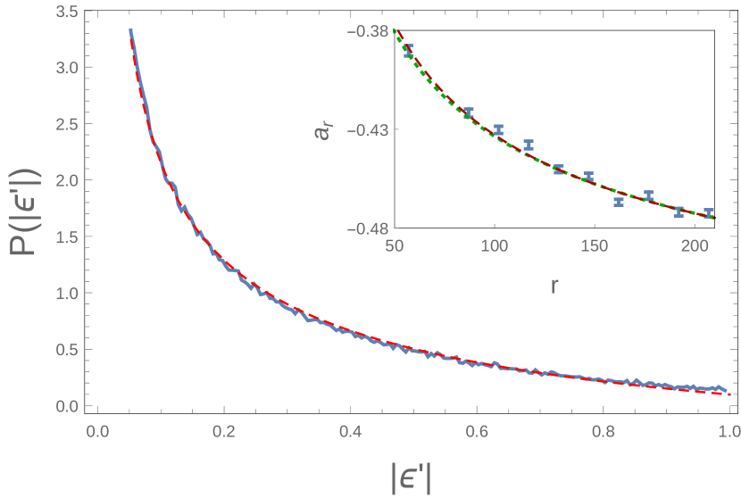
where labels the sites belonging to the optimal path . We find that the disorder-averaged IPR scales linearly with the length of the path , indicating that an extensive (in ) number of edges contributes to the total path weight, and cooperate to produce the atypically big path weights dominating (32). Fig. 14 shows the distribution of the absolute value of the energies along the optimal path for , , and . The fitting function has the form
| (54) |
The power-law behavior is consistent with the considerations in Ref. Yu and Müller, 2013. Adapting their reasoning to the finite dimensional case, one can argue that asymptotically in (and under the hypothesis of independent paths) the biased energy distribution along the optimal path has the form
| (55) |
with solving the -dependent equation
| (56) |
Fitting the -dependence of the coefficients one finds that the asymptotic limits are in agreement with (55); for details see the inset of Fig. 14.
IV.2 The many-body case
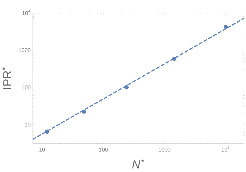
When performing the same type of analysis for the Heisenberg chain, we find that the statistics of the sum (46) is not well reproduced by the optimal path alone: the distribution of the ratios between the full sum and the optimal path is very wide and peaked at values that are far from one. Thus, despite also in this case the amplitude of the single paths are fat-tailed distributed, there is not a single one dominating. Instead, we find that the average IPR* of the paths amplitudes (which we denote with ):
| (57) |
scales linearly with the total number of paths , indicating that there are factorially many (in the length of the chain ) paths having amplitudes that are comparable in absolute value. This is a signature of the strong correlations between the paths, which is not surprising in view of the many-body nature of the model. Following Ref. Ros et al., 2015, one can argue that the strongest correlations are among those paths associated to processes in which the same spin flips occur, but in different order: the different orderings of the flips produce different energy denominators in (46), and thus different path amplitudes; however, the resulting terms are correlated, and one can expect that for those realizations of the random fields producing one particularly large path weight, the other ones (related to it by permutation of the order of the spin flips) will also have a large amplitude in absolute value. However, in the sum (46) the paths contribute with well defined relative signs, leading to cancellations between these factorially many terms (see Ref. Ros et al., 2015 for an explicit calculation for a model of interacting fermions), which are fully taken into account only with the transfer matrix method.
V Conclusion
In this work we have discussed the advantages and the limitations of the forward approximation applied to both single- and many-body quantum disordered systems. In particular, the FA has been used to obtain an expression for the wave functions, that can be computed by means of a transfer matrix technique. The statistical analysis of the wave functions allows to determine the critical values of the disorder (exact in large ), the critical exponents of the localization length (which turn out to be mean-field) and the universal distribution of the eigenfunctions’ coefficients.
For the single particle case, the amplitudes of the wave functions in FA turned out to be very well approximated by only one path, the dominating path: this has been exploited to investigate larger system sizes with respect to the ones accessible with the transfer matrix (the algorithm that computes the best path runs in time linear in the number of edges of the underlying graph, and is not as memory-demanding as either the transfer matrix of shift-invert exact diagonalization). The extremely good agreement (within statistical error) of the predicted critical values for the disorder for suggests that the approximation should be predictive also for the properties of the wave functions at the critical point. We have not investigated in details these implications, but we foresee the wave functions to have a sparse structure which is similar to that discussed in high-coordination Bethe latticesDe Luca et al. (2014). The strong similarities with the problem of directed polymers in random medium have also been addressed; however, from the statistical analysis it emerges that the scaling exponents describing the fluctuations of the wave functions are non-mean field, but also not equal to those of the directed polymer. Moreover, the limiting distribution of the appropriately rescaled wave functions seems to depend weaker on the dimensionality with respect to the directed polymer case.
In many-body problem there is no concentration of amplitude on a small number of paths, but there are strong cancellations between them: as a result, the full sum over factorially-many paths is only exponentially large (or small) in the system size. The correlation between the paths has been discussed in detail in Ref. Ros et al., 2015, and this work can be interpreted as a numerical test of the claims in that work. For the XXZ chain with random fields, the critical value predicted within the approximation () is very close to the most updated result obtained with exact diagonalization; thus, this tool furnishes an alternative route to exact diagonalization, that can be applied to significantly larger system sizes. We leave to future work the question of how to incorporate higher-order corrections in the FA within the transfer matrix scheme, and how they affect the critical exponents, and the accuracy of the results.
As a conclusive remark, we would like to briefly comment on the nature of the FA as a mean-field approximation for Anderson localization. For certain, the value of the critical disorder for the onset of localization grows indefinitely with , and in high the hopping becomes an almost negligible perturbation at the transition. The fact that the error in essentially disappears around is a strong indication of this. This feature is quite peculiar, since in ordinary, second order phase transitions the critical exponents above the upper critical dimension are correctly reproduced by the mean field approximation, but the location of the transition (e.g. the critical temperature) is not. In this sense the locator expansion (that to lowest order reduces to the FA considered in this work) becomes a better suited candidate for a mean field than the expansion of the nonlinear supersymmetric sigma model (NLSM)Efetov (1999). It is plausible that there is a field-theoretical description of the FA which can be put in direct relation with the NLSM; this is an obvious direction in which to continue this work. In addition, the relation with the Bethe lattice results can be further investigated, given that the critical predicted by the FA does not correspond to that of a Bethe lattice of any (integer) coordination number.
VI Acknowledgements
AS would like to thank B.L.Altshuler, R.Moessner, V.Oganesyan and S.L.Sondhi for discussions.
Appendix A Probability density of
An estimate for the probability density of can be obtained making use of the fact that the sum over (33) is dominated by the single path with maximal weight:
| (58) |
If the correlations between the different path weights are neglected, the calculation is similar to the one performed for the Bethe lattice case. In particular, one finds for the cumulative function of the following expression:
| (59) |
where is the total number of paths on which the maximum is taken. This implies the following form for the probability density of :
| (60) |
where we introduced the monotone decreasing function
| (61) |
The typical value of , denoted , is defined by the equation
| (62) |
The solutions of (62) approach a finite limit for , which is related to the critical value of disorder by , as previously discussed. Using that and computing the integral in (62) with a saddle point calculation (assuming ), one recovers the condition (28) for , with the substitution .
For increasing the probability density of peaks at the typical value, with tails that approach zero in the limit . In particular, for the decay of the tail is exponential in . Indeed, in this regime the product is itself exponentially decreasing with ; thus, the rightmost exponential in (60) rapidly converges to one, and the distribution approaches zero with a tail of the form
| (63) |
When becomes smaller than the typical value , the product increases exponentially. Since for large the integral is still exponentially small for all , one can still set . Thus, in this regime the probability density of decays to zero much faster, double-exponentially with
| (64) |
Note that (for large enough) the interval in which does not shrink to zero for , given that the value obtained from the condition (62) is always bigger than one. When approaches one, the probability in (61) is no longer a large deviation probability, i.e. it is no longer exponentially small in : the term approaches a constant function of , and the main scaling is given by the factor .
Finally, exactly at , using (62) and performing the integral with an integration by parts, one finds that the probability density can be written as
| (65) |
which diverges like when .
Given the tails of the distribution of computed in this approximation, it is immediate to derive the asymptotic decay of the probability of resonances in the localized phase. Indeed, for , the probability (35) is is a large deviation for . Making use of (63) we find
| (66) |
with
| (67) |
Thus, within this approximation for approaching from above one finds
| (68) |
thus the length scale diverges at the transition with a critical exponent equal to .
References
- Abrahams (2010) E. Abrahams, 50 years of Anderson localization, Vol. 24 (World Scientific, 2010).
- Billy et al. (2008) J. Billy, V. Josse, Z. Zuo, A. Bernard, B. Hambrecht, P. Lugan, D. Clément, L. Sanchez-Palencia, P. Bouyer, and A. Aspect, Nature 453, 891 (2008).
- Roati et al. (2008) G. Roati, C. D’Errico, L. Fallani, M. Fattori, C. Fort, M. Zaccanti, G. Modugno, M. Modugno, and M. Inguscio, Nature 453, 895 (2008).
- Anderson (1958) P. Anderson, Phys. Rev. 109, 1492 (1958).
- Evers and Mirlin (2008) F. Evers and A. D. Mirlin, Reviews of Modern Physics 80, 1355 (2008).
- Basko et al. (2006) D. Basko, I. Aleiner, and B. Altshuler, Annals of physics 321, 1126 (2006).
- Oganesyan and Huse (2007) V. Oganesyan and D. Huse, Physical Review B 75, 155111 (2007).
- Pal and Huse (2010) A. Pal and D. A. Huse, Phys. Rev. B 82, 174411 (2010).
- De Luca and Scardicchio (2013) A. De Luca and A. Scardicchio, Europhys. Lett. 101, 37003 (2013).
- Serbyn et al. (2013) M. Serbyn, Z. Papić, and D. A. Abanin, Physical review letters 111, 127201 (2013).
- Imbrie (2014) J. Z. Imbrie, arXiv preprint arXiv:1403.7837 (2014).
- Kjäll et al. (2014) J. A. Kjäll, J. H. Bardarson, and F. Pollmann, Physical review letters 113, 107204 (2014).
- Huse et al. (2014) D. A. Huse, R. Nandkishore, and V. Oganesyan, Physical Review B 90, 174202 (2014).
- Laumann et al. (2014) C. Laumann, A. Pal, and A. Scardicchio, Physical review letters 113, 200405 (2014).
- Chandran et al. (2015) A. Chandran, I. H. Kim, G. Vidal, and D. A. Abanin, Physical Review B 91, 085425 (2015).
- Ros et al. (2015) V. Ros, M. Müller, and A. Scardicchio, Nuclear Physics B 891, 420 (2015).
- Luitz et al. (2015) D. J. Luitz, N. Laflorencie, and F. Alet, Physical Review B 91, 081103 (2015).
- Altshuler et al. (1997) B. Altshuler, Y. Gefen, A. Kamenev, and L. Levitov, Phys. Rev. Lett. 78, 2803 (1997).
- Huse et al. (2015) D. A. Huse, R. Nandkishore, F. Pietracaprina, V. Ros, and A. Scardicchio, Phys. Rev. B 92, 014203 (2015).
- Abou-Chacra et al. (1973) R. Abou-Chacra, D. Thouless, and P. Anderson, Journal of Physics C: Solid State Physics 6, 1734 (1973).
- Medina and Kardar (1992) E. Medina and M. Kardar, Physical Review B 46, 9984 (1992).
- De Luca et al. (2014) A. De Luca, B. Altshuler, V. Kravtsov, and A. Scardicchio, Physical review letters 113, 046806 (2014).
- Note (1) A similar argument gives a perturbative series in for the conductance.
- Note (2) Evidence for the fact that this finite limit is indeed approached in the limit of large is provided in the numerical calculations below.
- Abou-Chacra and Thouless (1974) R. Abou-Chacra and D. Thouless, Journal of Physics C: Solid State Physics 7, 65 (1974).
- Nguyen et al. (1985a) V. Nguyen, B. Spivak, and B. Shklovskii, JETP Lett 41 (1985a), [Pis’ma Zh. Eksp. Teor. Fiz. 41, 35 (1985)].
- Nguyen et al. (1985b) V. Nguyen, B. Spivak, and B. Shklovskii, Sov. Phys.—JETP 62, 1021 (1985b), [Zh. Eksp. Teor. Fiz. 89, 11 (1985).
- Nguyen et al. (1986) V. Nguyen, B. Spivak, and B. Shklovskii, JETP Lett 43 (1986), [Pis’ma Zh. Eksp. Teor. Fiz. 43, 35 (1986)].
- Note (3) Note that the present calculation does not reduce to the one for the NSS case, since a major difference between the two models is in the statistics of energy denominators: in the NSS model the binary disorder (with probability or ) does not allow for resonances due to a single site. Rather, the resonances arise from contributions of different paths. This led to a body of work following Ref. \rev@citealpnumMedina1992, on the presence of a sign transition, where effects from different paths accumulate in order to break the sign symmetry. In the FA for the Anderson case, the energy denominators can be arbitrarily small with finite probability, generating path weights that are fat tailed distributed. The fat tail of this distribution is crucial for the considerations below.
- Monthus and Garel (2012) C. Monthus and T. Garel, Journal of Physics A: Mathematical and Theoretical 45, 095002 (2012).
- Slevin and Ohtsuki (2014) K. Slevin and T. Ohtsuki, New Journal of Physics 16, 015012 (2014).
- Ueoka and Slevin (2014) Y. Ueoka and K. Slevin, Journal of the Physical Society of Japan 83, 084711 (2014).
- García-García and Cuevas (2007) A. M. García-García and E. Cuevas, Phys. Rev. B 75, 174203 (2007).
- Derrida (1990) B. Derrida, Physica A Statistical Mechanics and its Applications 163, 71 (1990).
- Derrida and Spohn (1988) B. Derrida and H. Spohn, Journal of Statistical Physics 51, 817 (1988).
- Halpin-Healy and Zhang (1995) T. Halpin-Healy and Y.-C. Zhang, Physics reports 254, 215 (1995).
- Somoza et al. (2007) A. M. Somoza, M. Ortuño, and J. Prior, Phys. Rev. Lett. 99, 116602 (2007).
- Prior et al. (2009) J. Prior, A. M. Somoza, and M. Ortuño, The European Physical Journal B 70, 513 (2009).
- Somoza et al. (2015) A. M. Somoza, P. Le Doussal, and M. Ortuño, Phys. Rev. B 91, 155413 (2015).
- Monthus and Garel (2009) C. Monthus and T. Garel, Phys. Rev. B 80, 024203 (2009).
- Feigel’man et al. (2010) M. V. Feigel’man, L. B. Ioffe, and M. Mézard, Phys. Rev. B 82, 184534 (2010).
- Ioffe and Mézard (2010) L. B. Ioffe and M. Mézard, Phys. Rev. Lett. 105, 037001 (2010).
- Müller (2013) M. Müller, EPL (Europhysics Letters) 102, 67008 (2013).
- Yu and Müller (2013) X. Yu and M. Müller, Annals of Physics 337, 55 (2013).
- Note (4) Note that if this constraint is relaxed and the energy denominators are allowed to be arbitrarily small, is found to be proportional to the quantity that we are considering.
- Medina et al. (1989) E. Medina, M. Kardar, Y. Shapir, and X. R. Wang, Phys. Rev. Lett. 62, 941 (1989).
- Fisher and Huse (1991) D. S. Fisher and D. A. Huse, Phys. Rev. B 43, 10728 (1991).
- Huse et al. (1985) D. A. Huse, C. L. Henley, and D. S. Fisher, Phys. Rev. Lett. 55, 2924 (1985).
- Johansson (2000) K. Johansson, Communications in Mathematical Physics 209, 437 (2000).
- Prähofer and Spohn (2000) M. Prähofer and H. Spohn, Phys. Rev. Lett. 84, 4882 (2000).
- Prähofer and Spohn (2002) M. Prähofer and H. Spohn, Journal of statistical physics 108, 1071 (2002).
- Prähofer and Spohn (2004) M. Prähofer and H. Spohn, Journal of statistical physics 115, 255 (2004).
- Žnidarič et al. (2008) M. Žnidarič, T. Prosen, and P. Prelovšek, Physical Review B 77, 64426 (2008).
- Bardarson et al. (2012) J. H. Bardarson, F. Pollmann, and J. E. Moore, Phys. Rev. Lett. 109, 017202 (2012).
- Bauer and Nayak (2013) B. Bauer and C. Nayak, J. Stat. Mech 2013, P09005 (2013).
- Nanduri et al. (2014) A. Nanduri, H. Kim, and D. A. Huse, Phys. Rev. B 90, 064201 (2014).
- Bar Lev et al. (2015) Y. Bar Lev, G. Cohen, and D. R. Reichman, Phys. Rev. Lett. 114, 100601 (2015).
- (58) I. Mondragon-Shem, A. Pal, T. L. Hughes, and C. R. Laumann, arXiv:1501.03824 [cond-mat.dis-nn] .
- Goold et al. (2015) J. Goold, S. R. Clark, C. Gogolin, J. Eisert, A. Scardicchio, and A. Silva, arXiv:1504.06872 [cond-mat.dis-nn] (2015).
- Buccheri et al. (2011) F. Buccheri, A. De Luca, and A. Scardicchio, Physical Review B 84, 094203 (2011).
- Biroli et al. (2012) G. Biroli, A. Ribeiro-Teixeira, and M. Tarzia, arXiv preprint arXiv:1211.7334 (2012).
- De Luca et al. (2013) A. De Luca, A. Scardicchio, V. E. Kravtsov, and B. L. Altshuler, arXiv:1401.0019 (2013).
- Dijkstra (1959) E. Dijkstra, Numerische Mathematik 1, 269 (1959).
- Efetov (1999) K. Efetov, Supersymmetry in disorder and chaos (Cambridge University Press, 1999).