Optimizing Quantum Adiabatic Algorithm

Abstract

In quantum adiabatic algorithm, as the adiabatic parameter $s(t)$ changes slowly from zero to one with finite rate, a transition to excited states inevitably occurs and this induces an intrinsic computational error. We show that this computational error depends not only on the total computation time $T$ but also on the time derivatives of the adiabatic parameter $s(t)$ at the beginning and the end of evolution. Previous work (Phys. Rev. A 82, 052305) also suggested this result. With six typical paths, we systematically demonstrate how to optimally design an adiabatic path to reduce the computational errors. Our method has a clear physical picture and also explains the pattern of computational error. In this paper we focus on quantum adiabatic search algorithm although our results are general.

I Introduction

Quantum adiabatic algorithm was proposed in 2000 by Farhi et al.Farhi0 as an alternative paradigm of quantum computing to quantum circuit algorithm QuantumComputationBook . It works by constructing a time-dependent Hamiltonian that evolves slowly from the initial Hamiltonian to the problem Hamiltonian. The ground state of the initial Hamiltonian is easy to find and the answer of the intent problem is encoded in the problem Hamiltonian. It is ensured by the quantum adiabatic theorem that if the Hamiltonian evolves slowly enough, the system will stay in the ground state and evolve into the ground state of the problem Hamiltonian. When it is applied to the search problem, the quantum adiabatic algorithm has been shown to be $O(\sqrt{N})$ Roland ; RezakhaniPRL , which is as powerful as Grover’s algorithm Grover and is quadratic speedup over the classical search algorithm. In general, the adiabatic algorithm has been shown to have the potential to solve NP-hard problem Farhi2 ; Zhuang .

In addition to its speed up against classical computing, the quantum adiabatic algorithm also has capacity to remain robust against environment noise Preskill . Some practical architectures for quantum adiabatic algorithms were proposed Seth ; in 2013 D-Wave company claimed that they built a quantum computer based on quantum adiabatic algorithm DWAVE .

In quantum adiabatic algorithm, there are two types of computational errors. One is the extrinsic error, which is caused by the environment. The other is the intrinsic error: as the algorithm has to be run in a finite computation time $T$, the adiabatic Hamiltonian must change in a finite rate and this inevitably will induce transition to excited states and cause computational error. The intrinsic computational error depends entirely on how the adiabatic path $s(t)$ is chosen. The most popular choice so far is the linear path, $s(t)=t/T$. Other choices were proposed in literature Rezakhani . People has also tried to optimize the adiabatic path $s(t)$ using geometrization RezakhaniPRL .

According to the hierarchical theory of quantum adiabatic evolution Qi , the intrinsic error depends crucially on the time derivatives of $s(t)$ at the beginning and the end of the evolution. This fact was also pointed out in Ref. Rezakhani ; Lidar . In this work we choose six typical adiabatic paths $s(t)$ to systematically demonstrate how to optimally control these time derivatives to reduce the computational error. Also we give a physical picture about the origin of computational error’s oscillation. We focus on the quantum adiabatic search algorithm and numerically compare the computational errors for different adiabatic paths. We find that the cubic path is the best among the six chosen path and it can reduce the error by orders of magnitude compared to the popular linear path and sinusoidal path.

Our paper is organized as follows: for the sake of self-containment, we first briefly introduce the quantum adiabatic algorithm, in particular, the quantum adiabatic search algorithm, and the hierarchical theory of quantum adiabatic evolution, respectively, in Sections II and III. In Section IV, we show that the Hamiltonian for the quantum adiabatic search algorithm can be reduced to a spin-1/2 Hamiltonian and apply the hierarchical theory. In Section V, six typical adiabatic paths are chosen and they are categorized into three groups. Our main numerical results are shown in Section VI. We finally conclude in Section VII.

II Quantum Adiabatic Search Algorithm

The adiabatic quantum computation was first introduced in 2000 Farhi0 based on the quantum adiabatic theorem BornFock . In a quantum adiabatic algorithm, the solution of a problem is encoded into the ground state of the problem Hamiltonian $H_{p}$. An initial Hamiltonian $H_{b}$ is chosen so that its ground state can be easily found and set up. The total adiabatic Hamiltonian is constructed by linking the initial Hamiltonian with the problem Hamiltonian with a path as follows

$$H_{s}(t)=(1-s(t))H_{b}+s(t)H_{p}\,,$$ (1)

where $s(t)\in[0,1]$ is the adiabatic parameter. The system is prepared in the ground state of $H_{b}$. As $s$ changes slowly from zero to one, the quantum adiabatic theorem ensures that the system stays in the ground state of $H_{s}$ and eventually arrives at the ground state of $H_{p}$, the solution.

In the search problem, the task is to locate $M$ marked items out of $N$ randomly arranged items. On a quantum computer, we use a set of orthonormal basis $|1\rangle,|2\rangle,...,|N\rangle$ to denote the $N$ unsorted items. The problem Hamiltonian can be constructed as Roland

$$H_{p}=1-\sum_{m\in\mathcal{M}}|m\rangle\langle m|,$$ (2)

where $\mathcal{M}$ is the set of marked items. This Hamiltonian is the projection operator to a subspace orthogonal to the subspace spanned by $\{|m\rangle\}_{m\in\mathcal{M}}$; its ground state can be any state from subspace $\{|m\rangle\}_{m\in\mathcal{M}}$. If we choose the initial state to be equally contributed from the orthonormal basis as $|\psi_{0}\rangle=\dfrac{1}{\sqrt{N}}\sum_{i=1}^{N}|i\rangle$, then the initial Hamiltonian is

$$H_{b}=1-|\psi_{0}\rangle\langle\psi_{0}|=1-\dfrac{1}{N}\sum_{i,j}|i\rangle\langle j|.$$ (3)

Thus the quantum adiabatic Hamiltonian for search is

$$H_{s}=1-\dfrac{1-s(t)}{N}\sum_{i,j}|i\rangle\langle j|-s(t)\sum_{m\in\mathcal{M}}|m\rangle\langle m|\,.$$ (4)

Note that the unit of Hamiltonian which rules the quantum computation depends on what kind of system is used for realization. Suppose a system has a characteristic time $\tau$; the unit of Hamiltonian is $\hbar/\tau$. For convenience, in the following derivation, we set $\tau=\hbar=1$.

In the above Hamiltonian, if $s(t)$ changes from zero to one infinitely slowly, the system will stay strictly in the ground state and the solution can be found without any error if there is no environment noise. This is dictated by the quantum adiabatic theorem. However, we want to know the solution as fast as possible. This means that $s$ has to change from zero to one in a finite time $T$, causing a small transition to excited states. At the end, there is an inevitable error in the solution. For the search problem, we define the intrinsic computational error as Rezakhani

$$\delta=1-\langle\psi(T)|\hat{P}|\psi(T)\rangle\,,$$ (5)

where the projection operator $\hat{P}$ is defined as

$$\hat{P}=\sum_{m\in\mathcal{M}}|m\rangle\langle m|\,.$$ (6)

The main purpose of this work is to reduce the computational error $\delta$ by optimizing the adiabatic path $s(t)$. The simplest and also the most popular choice is the linear path $s=t/T$. This is almost the worst among the easy choices, which includes sinusoidal path. According to the newly developed hierarchical theory of quantum adiabatic evolution Qi , the error $\delta$ depends crucially how the time derivatives of $s(t)$ at the beginning and the end of the adiabatic evolution. In this work, several adiabatic paths $s(t)$ are designed and the errors caused by these paths are computed and compared to the error by the linear path. The error can be reduced by orders of magnitude.

III Hierarchical Theory of Quantum Adiabatic Evolution

Figure 1: (color online)Adiabatic evolution trajectories in the projective Hilbert space. The red lines are the zeroth-order trajectories, that is, the trajectories follow strictly the quantum adiabatic theorem. The blue lines are the first-order trajectories, which are shifted from the zeroth-order ones by a small amount proportional to $\dot{s}$. The black lines are the second-order trajectories. When $\dot{s}$ is not zero at $t=0$, the system will oscillate around the first-order trajectory (the green line in (a)). Similarly, when $\ddot{s}$ is not zero at $t=0$, the system will oscillate around the second-order trajectory (the green line in (b)).

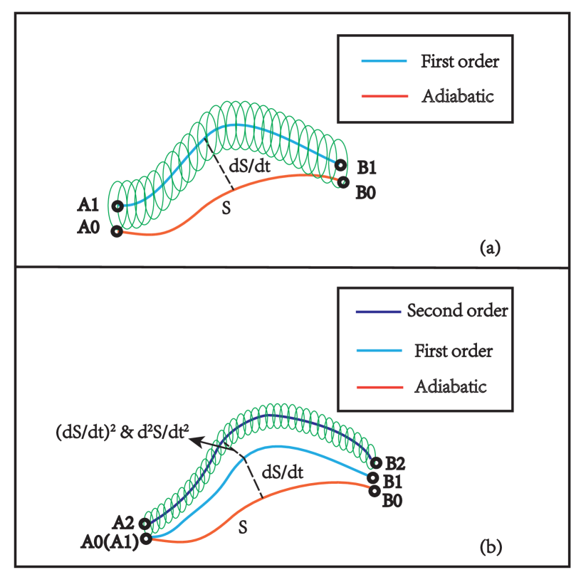
The quantum adiabatic theorem was proved in 1928 by Born and Fock BornFock . This theorem ensures that a system starting in the ground state will stay in the ground state when the adiabatic parameter $s$ changes slowly. However, this is mathematically true only when the changing rate of $s$ is infinitesimally small. In any practical situation, for example, quantum adiabatic computing, the adiabatic parameter $s$ has to change with a small but finite rate, this will cause a small transition to excited states, resulting a deviation from the quantum adiabatic theorem. In Ref. Qi , a hierarchical theory was developed to compute the deviation order by order.

The results are schematically illustrated in Fig. 1 with trajectories in the projective Hilbert space (the overall phase is not important) Fu1 ; Fu2 ; Niu . At the zeroth order, the system follows the trajectory dictated by the quantum adiabatic theorem. At the first order, the system oscillates with a small amplitude around a trajectory slightly shifted from the zeroth-order trajectory. The small shift is proportional to $\dot{s}$, the first-order time derivative of $s(t)$; the small oscillating amplitude is determined by $\dot{s}$ at $t=0$. This is illustrated in Fig. 1(a).

To reduce and also to better control the computational error $\delta$, we can set $\dot{s}=0$ at the beginning. In this case, there are no oscillations and the system will follow a smooth first-order trajectory. As the shift between the first-order trajectory and the zeroth-order trajectory is proportional to $\dot{s}$, we can reduce the error $\delta$ in the first order to zero by choosing a $s(t)$ such that $\dot{s}=0$ at $t=T$. For such a path $s(t)$, the error $\delta$ is of the second-order, determined by $\ddot{s}$, the second-order time derivative of $s(t)$. To further reduce the error, we can repeat the above procedure by choosing a path $s(t)$ such that $\ddot{s}=0$ at $t=0,T$. This strategy is very successful as we shall see in the following sections.

We note here that the crucial role played by the time derivatives was also pointed out in Ref. Rezakhani ; Lidar with a different approach.

IV Reduced Search Hamiltonian and Analytical Results

Let us come back to the search Hamiltonian and see how the hierarchical theory outlined in the last section can be applied successfully to this problem. Because of the permutation symmetry of the search Hamiltonian $H_{s}$, for the given initial state, the quantum state at any given time has the form VDam2

$$|\psi\rangle=\frac{\psi_{u}}{\sqrt{N-M}}\sum_{u\notin\mathcal{M}}|u\rangle+\frac{\psi_{m}}{\sqrt{M}}\sum_{m\in\mathcal{M}}|m\rangle\,.$$ (7)

The Schrödinger equation governing the search algorithm becomes

$$i\dfrac{\partial}{\partial t}\begin{pmatrix}\psi_{u}\\ \psi_{m}\end{pmatrix}=\widetilde{H}_{s}\begin{pmatrix}\psi_{u}\\ \psi_{m}\end{pmatrix},$$ (8)

with

$$\widetilde{H}_{s}=\begin{pmatrix}r(1-s(t))+s&-\sqrt{r(1-r)}(1-s(t))\\ -\sqrt{r(1-r)}(1-s(t))&(1-r)(1-s(t))\end{pmatrix}$$ (9)

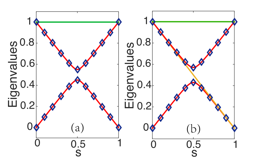
where $r=M/N$. In other words, the search Hamiltonian $H_{s}$ is reduced to a spin-1/2 Hamiltonian $\widetilde{H}_{s}$. Fig. 2 shows the eigenvalues of both Hamiltonians, $H_{s}$ and $\widetilde{H}_{s}$. It is clear that two eigenvalues of $\widetilde{H}_{s}$ (diamonds) are identical to two of the eigenvalues of $H_{s}$ (red solid lines). Due to the permutation symmetry, all other eigenstates of $H_{s}$ (non-red solid lines) do not participate in the dynamical evolution when $s$ changes from zero to one.

Figure 2: (color online)Eigenvalues of the search Hamiltonian. (a) $N=100$, $M=1$; (b) $N=100$, $M=2$. The solid lines are for $H_{s}$ and the diamonds for $\widetilde{H}_{s}$. The time unit depends on the system used to realize our algorithm. Suppose the system has a characteristic time $\tau$, then the unit of energy is $\hbar/\tau$. In this article, we have set $\hbar=\tau=1$.

To apply the hierarchical theory in Ref.Qi , we reformulate our problem in the projective Hilbert space Fu1 ; Fu2 ; Niu . We rewrite the state as

$$|\psi_{2}\rangle=\begin{pmatrix}\psi_{u}\\ \psi_{m}\end{pmatrix}=\dfrac{\lambda_{1}}{\sqrt{2}}\begin{pmatrix}1\\ i\end{pmatrix}+\dfrac{\lambda_{2}}{\sqrt{2}}\begin{pmatrix}1\\ -i\end{pmatrix}\,,$$ (10)

and define $p=\arg(\lambda_{2})-\arg(\lambda_{1})\in[0,2\pi]$, $q=|\lambda_{2}|^{2}\in[0,1]$. The dynamics of our system in the projective Hilbert space can be completely determined by $p$ and $q$. In terms of $p$ and $q$, the classical Hamiltonian becomes

$$\widetilde{H}_{c} = \dfrac{1}{2}+\sqrt{q(1-q)}\cos(p)(2r+2s-2rs-1)$$ (11)

$$-2\sqrt{q(1-q)}\sin(p)\sqrt{r(1-r)}(1-s)\,,$$

where $\widetilde{H}_{c}=\langle\psi_{2}|\widetilde{H}_{s}|\psi_{2}\rangle$.

The ground state of the reduced search Hamiltonian is a fixed point in the projective Hilbert space where the overall phase is removed. The fixed point is given by

$$\left\{\begin{array}[]{ll}\bar{q}=\dfrac{1}{2}\\ \bar{p}=\left\{\begin{array}[]{ll}\pi-\arctan(\dfrac{2\sqrt{(1-r)r}(1-s)}{2r+2s-2rs-1}).~{}~{}(s\geq\dfrac{1-2r}{2-2r})\\ \\ \arctan(\dfrac{2\sqrt{(1-r)r}(1-s)}{2rs-2r-2s+1}).~{}~{}(s<\dfrac{1-2r}{2-2r})\end{array}\right.\end{array}\right.$$ (12)

where we have assumed that $r\ll 1$. When $s$ changes infinitesimally slowly, this fixed point traverses the adiabatic trajectory (the red lines in Fig. 1). When $s$ changes with a finite but small rate, the actual dynamics will deviate from the adiabatic trajectory of the fixed point. The averaged first-order and second-order deviations areQi

1. First Order Deviation
   

   $$\begin{pmatrix}A_{1}\\ B_{1}\end{pmatrix}=\begin{pmatrix}0\\ \dfrac{\dot{s}\sqrt{r(1-r)}}{\lambda^{3/2}}\end{pmatrix}$$ (13)

2. Second Order Deviation
   

   $$\begin{pmatrix}A_{2}\\ B_{2}\end{pmatrix}=\begin{pmatrix}2\sqrt{r(1-r)}\dfrac{3\dot{s}(r-1)(2-4s)-\lambda\ddot{s}}{\lambda^{3}}\\ 0\end{pmatrix}$$ (14)

where $\lambda=1+4(r-1)s-4(r-1)s^{2}$. $A_{i}$ is the ith order deviation of p, and $B_{i}$ is the ith order deviation of q. Detailed derivation of ($A_{i},B_{i}$) can be found in the appendix. The first-order deviation as depicted by the blue lines in Fig. 1 is proportional to $\dot{s}$. The second-order deviation is depicted by the black line in Fig. 1(b) and it is proportional to $\ddot{s}$ if $\dot{s}$ is zero.

V Adiabatic Paths

We will show in the last two sections that the time derivatives of $s$ at the beginning and end play a crucial role in determining the computational errors. We define these time derivatives as

$$c_{n}\equiv\dfrac{d^{n}s}{dt^{n}}(0)~{}~{}\,,~{}~{}~{}~{}~{}~{}d_{n}\equiv\dfrac{d^{n}s}{dt^{n}}(T)\,.$$ (15)

With $c_{n}$ and $d_{n}$, we categorize the evolution paths in the following ways: the path is called $n$th-order if all of its $c_{m}$ and $d_{m}$ for $m\leq n$ are zero while either $c_{n}$ or $d_{n}$ are not zero. The zeroth-order path has either $c_{1}\neq 0$ or $d_{1}\neq 0$. We propose the following six adiabatic paths to illustrate our ideas:

1. Linear path

   $$s_{1}(t)=\left\{\begin{array}[]{lll}0~{}~{}~{}t<0\\ \dfrac{t}{T}~{}~{}~{}0\leq t<T\\ 1~{}~{}~{}t\geq T\end{array}\right.$$ (16)

2. Sinusoidal path

   $$s_{2}(t)=\left\{\begin{array}[]{lll}0~{}~{}~{}t<0\\ \sin(\frac{\pi t}{2T})~{}~{}~{}0\leq t<T\\ 1~{}~{}~{}t\geq T\end{array}\right.$$ (17)

3. Square path

   $$s_{3}(t)=\left\{\begin{array}[]{lll}0~{}~{}~{}t<0\\ 3(\frac{t}{T})^{2}-2(\frac{t}{T})^{3}~{}~{}~{}0\leq t<T\\ 1~{}~{}~{}t\geq T\end{array}\right.$$ (18)

4. Sinusoidal square path

   $$s_{4}(t)=\left\{\begin{array}[]{lll}0~{}~{}~{}t<0\\ \sin^{2}(\frac{\pi t}{2T})~{}~{}~{}0\leq t<T\\ 1~{}~{}~{}t\geq T\end{array}\right.$$ (19)

5. Sinusoidal cubic path

   $$s_{5}(t)=\left\{\begin{array}[]{lll}0~{}~{}~{}t<0\\ \sin^{3}(\frac{\pi t}{2T})~{}~{}~{}0\leq t<T\\ 1~{}~{}~{}t\geq T\end{array}\right.$$ (20)

6. Cubic path

   $$s_{6}(t)=\left\{\begin{array}[]{lll}0~{}~{}~{}t<0\\ 6(\frac{t}{T})^{5}-15(\frac{t}{T})^{4}+10(\frac{t}{T})^{3}~{}~{}~{}0\leq t<T\\ 1~{}~{}~{}t\geq T\end{array}\right.$$ (21)

Among these six paths, linear path and sinusoidal path are of zeroth order; the first-order paths are square path, sinusoidal square path, and sinusoidal cubic path; cubic path is second order. As we shall see, the higher-order path can lead to smaller computational error by orders of magnitude. Note that only linear path and sinusoidal path of those six paths were studied before. Rezakhani

Figure 3: (color online) Deviations from the ground state as a function of time for the linear path and the sinusoidal path. The analytical results for the first-order deviation are plotted for comparison. ($N=10$, $M=1$, $T=1000$)

VI Numerical Results

The Schrödinger equation (8) is solved numerically for the six adiabatic paths for various values of $T$. The results are analyzed, explained, and compared in this section. They convincingly show that higher-order paths can reduce computational errors by orders of magnitude.

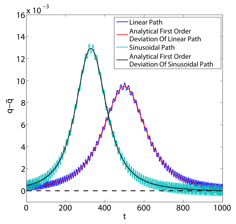
Fig. 3 shows how the deviation from the ground state (fixed point) changes with time for linear path and sinusoidal path. It is clear from this figure that the deviations oscillate around the first-order analytical results. And the amplitude of this oscillation is conserved, which is an result of conservation of actionDirac . This is expected from the hierarchical theory (see Fig. 1)Qi as both linear path and sinusoidal path are zeroth-order path with nonzero $c_{1}$. It is interesting to compare the results for linear path and sinusoidal path. The deviation for the sinusoidal path is larger than that for the linear path in the middle of the evolution; however, the computational error (i.e., the deviation at $t=T$) appears slightly smaller for sinusoidal path. The reason is that $\dot{s}$ decreases smoothly toward zero for the sinusoidal path. Although the reduction of the computational error is not much, it already shows the possibility to reduce the computational error by optimally designing $s(t)$ for a given $T$. This kind of reduction can be of order of magnitude when we choose a path of higher-order as we shall see next.

Figure 4: (color online) (a) Deviation from the ground state as a function of time for the square path. The analytical results for the second-order deviation are plotted for comparison. (b) Difference between numerical result of p and its second order analytical result as a function of time. ($N=10$, $M=1$, $T=1000$)

Figure 5: (color online) (a) Deviation from the ground state as a function of time for the square path. The analytical results for the second-order deviation are plotted for comparison. (b) Difference between numerical result of p and its second order analytical result as a function of time. ($N=10$, $M=1$, $T=1000$)

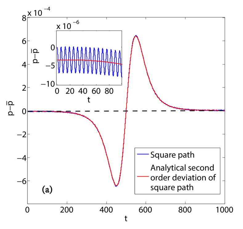
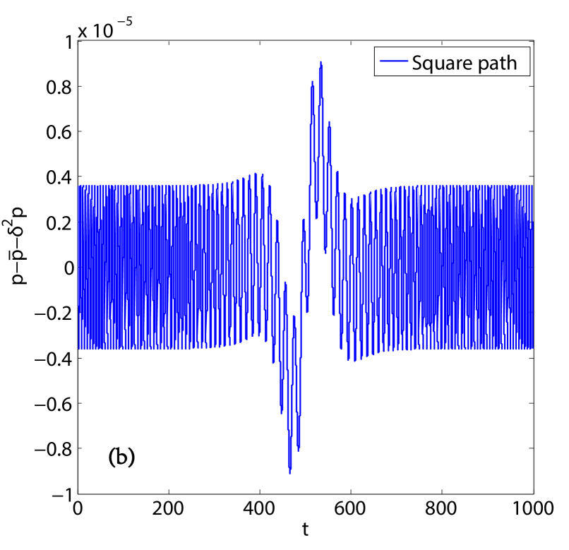
We have designed three first-order paths, square path, sinusoidal square path, and sinusoidal cubic path whose $c_{1}$ and $d_{1}$ are zero. As an example, our numerical results for square path is plotted in Fig.4. The results in Fig.4(a) are deviation from the ground state. As the first-order derivative $c_{1}$ and $d_{1}$ are zero, the deviation is of second order and it oscillates around the analytical second-order deviation (see the inset of Fig.4(a)). To see these oscillations more clearly, we have plotted the difference between our numerical results and the analytical second-order deviation in Fig.4(b)), where the oscillation pattern is seen to have a kink in the middle of the evolution. Since the second order derivatives $c_{2}$ and $d_{2}$ are very small, the deviation is very small, order of magnitude smaller than the ones in Fig. 3. The deviation pattern for sinusoidal square path and sinusoidal cubic path are similar to square path. To avoid the overcrowding of figures, we only plotted the results for square path.

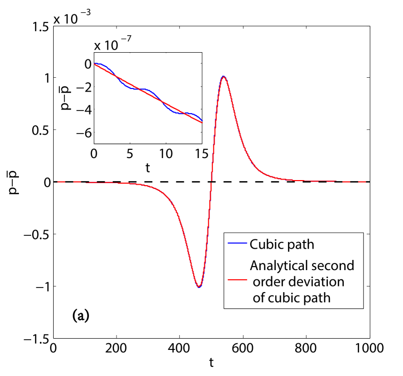
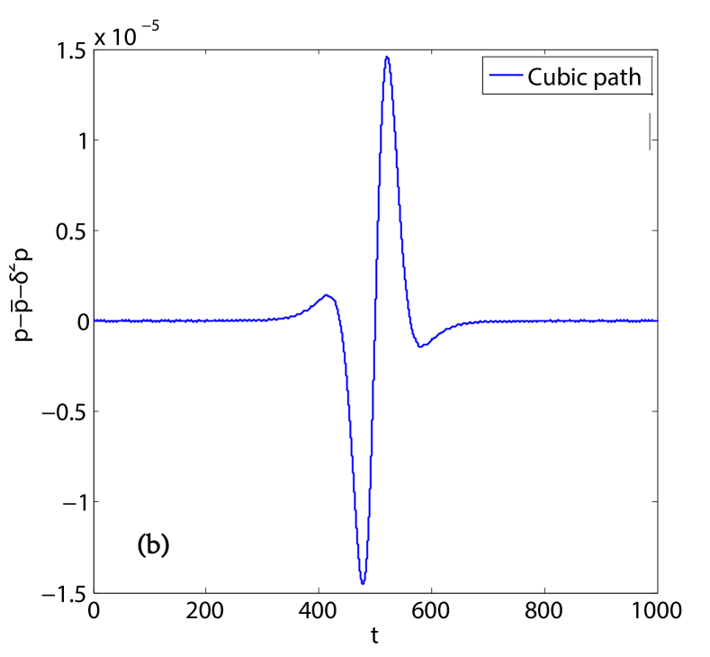
We finally look at the results for cubic path, which is the only second-order path among the six. From the discussion above, we know that the main deviation of cubic path is of the third order because both its $c_{2}$ and $d_{2}$ are zero. Therefore, the deviation of cubic path should be very different from square path. For comparison, the numerical results for cubic path are plotted in Fig.5 in a similar fashion as for square path. There are still oscillations around the second-order analytical result as seen from the inset of Fig.5(a). However, the oscillations have a very different pattern: as $c_{2}$ is zero, the oscillation starts at zero with a much smaller amplitude and frequency. In Fig.5(b), where the difference is plotted, the oscillations with small oscillations are not even visible due to a large kink around $t=500$. This is very different from Fig.4(b)). Overall, we see that the deviation of cubic path is much smaller than square path.

Figure 6: (color online) The computation error as a function of computation time $T$ for the linear path and the sinusoidal path. ($N=100$, $M=1$)

Figure 7: (color online) The computation error as a function of computation time $T$ for the square path, the sinusoidal square path, and the sinusoidal cubic path. ($N=100$, $M=1$)

Figure 8: (color online) The computation error as a function of computation time $T$ for the cubic path. ($N=100$, $M=1$)

Figure 9: (color online)The smoothed computational error with total evolution time of six paths. (N=100, M=1)

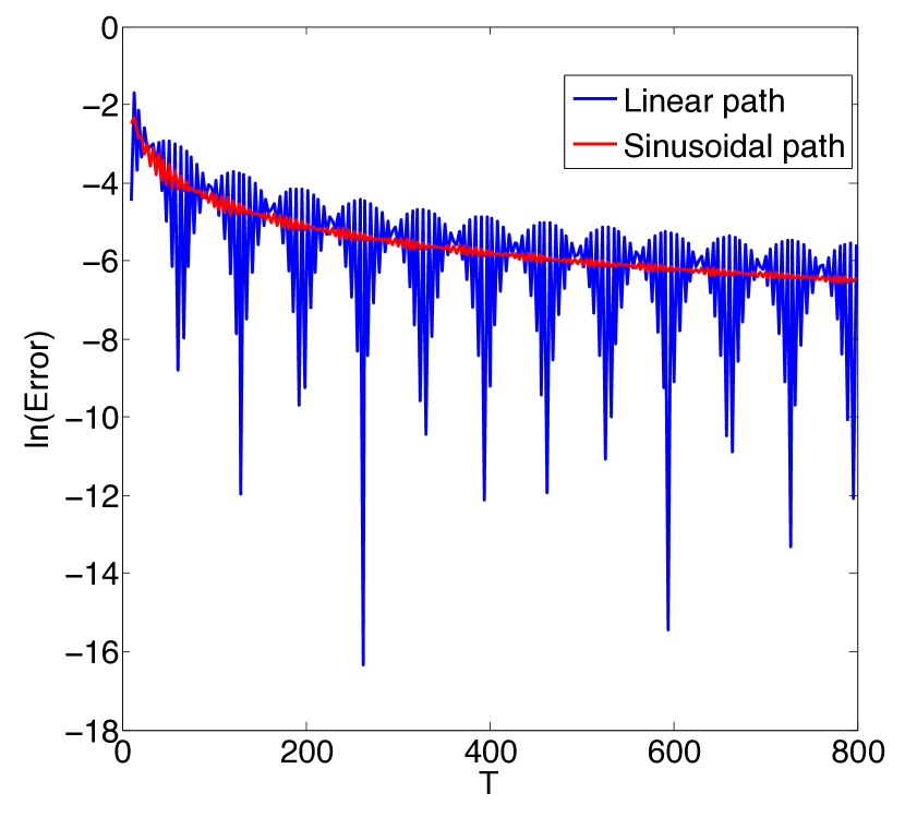
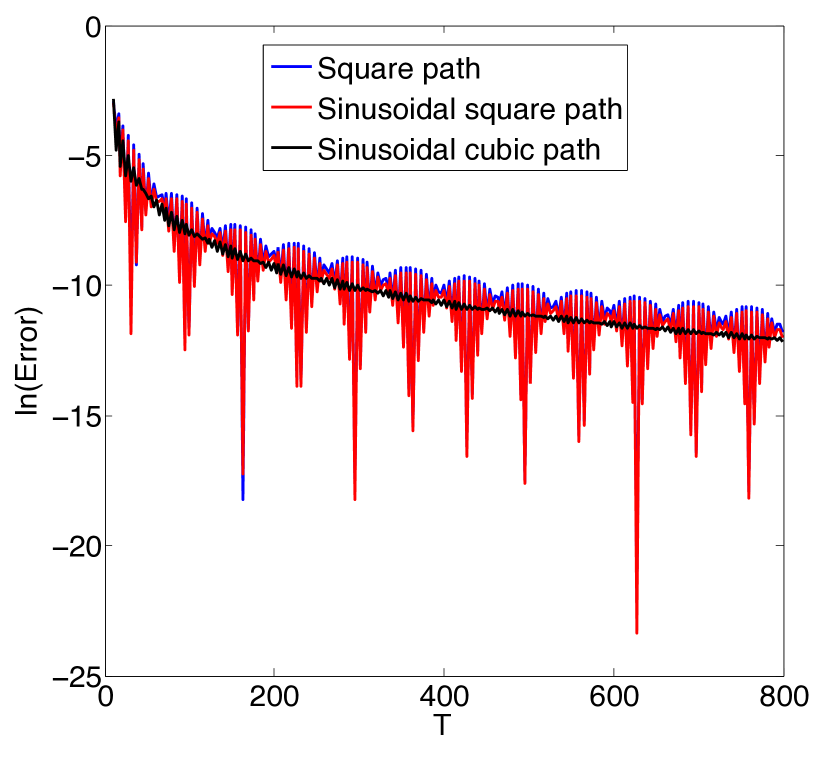
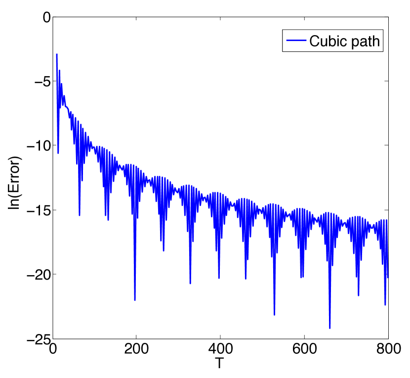
For a given total computation time $T$, the success of an algorithm depends on the computational error. The smaller the error the better the algorithm. The computational errors for all the six proposed paths are computed and plotted against the computation time $T$ in Figs. 6,7,&8. Fig. 6 shows the results for the two path of the zeroth order. The results for the three first-order paths are shown in Fig.7. The cubic path is of the second order and has the smallest computational error as seen in Fig. 8. The oscillations in these three figure are originated from the oscillations in Figs. 3&4; they are not essential.

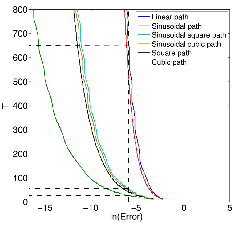
We can view the results in Figs. 6,7,&8 in a different angle: for a given allowed computational error, which path has the shortest computation time? For this angle, we have averaged out these oscillations and combined the results in Figs. 6,7&8 into Fig. 9. In Fig. 9, we see clearly that the relation between the computation time $T$ and the computational errors differs slightly for paths of the same order. However, for path of different orders, the relation is very different: for a certain allowed computational error, the computation time $T$ can differ by orders of magnitude; similarly, for a given computation time $T$, the error can differ by orders of magnitude. For example, at $T=100$, the computational error for cubic path is almost seven orders of magnitude smaller than the popular linear path. If we want to limit the computational error to $10^{-6}$, it only takes $T=25$ for cubic path; for sinusoidal square path, $T$ is around 46; for the popular linear path, it would take a much longer time $T=650$.

Although the oscillations are not essential, they do exhibit interesting patterns. The computational errors for four paths, the linear path, the square path, the sinusoidal square path, and the cubic path, have very similar oscillation patterns while the other two paths, the sinusoidal path and the sinusoidal cubic path, share another oscillation pattern. The pattern is largely depend on the relationship between $|c_{n}|$ and $|d_{n}|$, the derivatives of $s$ at the beginning and end. Take zeroth-order path as an example. If $|c_{1}|=|d_{1}|$, the actual trajectory can intersect the adiabatic trajectory for some values of $T$. At those $T$, the computational error is extremely small, as shown in Fig. 1(a). However, if $|c_{1}|\neq|d_{1}|$, the actual trajectory will oscillate with time but will not intersect the adiabatic trajectory. As a result, the computational error will have some oscillations but never reach zero.

Note that in this section we have chosen $N=10,~{}M=1$ for Figs. 3,4&5 just for the clarity of the figures. The essential conclusions drawn from these figures are the same for larger $N$.

VII Conclusion

In sum, with the aid of hierarchical theoryQi , we have shown that it is very effective to shrink the computational error by controlling the time derivative of $s(t)$ at the beginning and end of the evolution. Our numerical results with six typical adiabatic paths show that a path of higher orders (smoother path by intuition) leads to errors of orders of magnitude smaller. Or, for an allowed computational error, the algorithm with a higher-order path can be order-of-magnitude faster. The large deviation from the ground state in the middle of the evolution is not essential as long as it does not break the adiabaticity too much. Although we have focused on quantum search, our results and method are general and can be applied to other quantum adiabatic algorithms.

This work is supported by the NBRP of China (2013CB921903,2012CB921300) and the NSF of China (11274024,11334001,11429402).

Details on first order deviation

The first order deviation from instantaneous fixed points $(\bar{p},\bar{q})$ can be written as

$$p(t)=\bar{p}[s(t)]+\delta p,~{}~{}q(t)=\bar{q}[s(t)]+\delta q.$$ (22)

First we consider $s$ is fixed. Using Hamilton equations of motion and Talyor expansion to the first order of $(\delta p,\delta q)$, we have

$$\begin{pmatrix}\dfrac{dp}{dt}\\ \\ \dfrac{dq}{dt}\end{pmatrix}=\Gamma_{0}\begin{pmatrix}\delta p\\ \\ \delta q\end{pmatrix},$$ (23)

where

$$\Gamma_{0}=\begin{pmatrix}-\dfrac{\partial^{2}\widetilde{H}_{c}}{\partial q\partial p}&-\dfrac{\partial^{2}\widetilde{H}_{c}}{\partial q\partial q}\\ \\ \dfrac{\partial^{2}\widetilde{H}_{c}}{\partial p\partial p}&\dfrac{\partial^{2}\widetilde{H}_{c}}{\partial p\partial q}\end{pmatrix}_{p=\bar{p},q=\bar{q}}.$$ (24)

The reason why first-order derivatives of $\widetilde{H}_{c}$ do not appear on the right hand side of Eq.(23) is simply because $(\bar{p},\bar{q})$ is the fixed point.

Now we consider $s(t)$ changes slowly with time and examine the dynamics of $(\delta p,\delta q)$. We have

$$\begin{array}[]{l}\dfrac{dp}{dt}=\dfrac{\partial\bar{p}}{ds}\dot{s}+\dfrac{d\delta p}{dt}\\ \\ \dfrac{dq}{dt}=\dfrac{\partial\bar{q}}{\partial s}\dot{s}+\dfrac{d\delta q}{dt}.\end{array}$$ (25)

Eq.(23) becomes

$$\begin{pmatrix}\dfrac{d\delta p}{dt}\\ \\ \dfrac{d\delta q}{dt}\end{pmatrix}=\Gamma_{0}(s)\begin{bmatrix}\begin{pmatrix}\delta p\\ \\ \delta q\end{pmatrix}-\Gamma_{0}^{-1}(s)\begin{pmatrix}\dfrac{\partial\bar{p}}{\partial s}\\ \\ \dfrac{\partial\bar{q}}{\partial s}\end{pmatrix}\dot{s}\end{bmatrix}.$$ (26)

It can be shown that the determinant $|\Gamma_{0}|$ does not vanish as long as the energy levels of $\widetilde{H}_{s}$ are non degenerate. Previous workQi ; Fu1 ; Fu2 shows that $(\delta p,\delta q)$ are a canonical pair and Eq.(26) can be derived from following Hamiltonian,

$$\begin{array}[]{l}H_{1}(s,\dot{s})=\dfrac{1}{2}(\dfrac{\partial^{2}\widetilde{H}_{c}}{\partial q^{2}})_{\bar{p},\bar{q}}(\delta q-B_{1})^{2}+\\ \\ (\dfrac{\partial^{2}\widetilde{H}_{c}}{\partial q\partial p})_{\bar{q},\bar{q}}(\delta q-B_{1})(\delta p-A_{1})+\\ \\ \dfrac{1}{2}(\dfrac{\partial^{2}\widetilde{H}_{c}}{\partial p^{2}})_{\bar{p},\bar{q}}(\delta p-A_{1})^{2}\end{array},$$ (27)

where ($A_{1}$,$B_{1}$) is the center of first order deviation $(\delta p,\delta q)$ and defined as

$$\begin{pmatrix}A_{1}\\ \\ B_{1}\end{pmatrix}=\Gamma_{0}^{-1}(s)\begin{pmatrix}\dfrac{\partial\bar{p}}{\partial s}\\ \\ \dfrac{\partial\bar{q}}{\partial s}\end{pmatrix}\dot{s}.$$ (28)

Higher order derivations of ($p,q$) can be derived in similar way.

References

- (1) E. Farhi, J. Goldstone, S. Gutmann, and M. Sipser, arXiv:quant-ph/0001106v1 (2000).
- (2) M. A. Nielesn and I. L. Chuang, Quantum Computation and Quantum Information (Cambridge University Press, 2000).
- (3) J. Roland and N. J. Cerf, Phys. Rev. A 65, 042308 (2002).
- (4) A. T. Rezakhani, W.-J. Kuo, A. Hamma, D. A. Lidar, and P. Zanardi, Phys. Rev. Lett. 103, 080502 (2009).
- (5) L. K. Grover, Phys. Rev. Lett. 79, 325 (1997).
- (6) E. Farhi, J. Goldstone, S. Gutmann, J. Lapan, A. Lundgren, and D. Preda, Science 292, 472 (2001).
- (7) Q. Zhuang, Phys. Rev. A 90, 052317 (2014).
- (8) A. M. Childs, E. Farhi, and J. Preskill, Phys. Rev. A 65, 012322 (2001).
- (9) W. M. Kaminsky and S. Lloyd, arXiv:quant-ph/0211152v1 (2002).
-
(10)
http://www.dwavesys.com/
sites/default/files/Map%20Coloring%20WP2.pdf. - (11) A. T. Rezakhani, A. K. Pimachev, and D. A. Lidar, Phys. Rev. A 82, 052305 (2010).
- (12) Q. Zhang, J. Gong, and B. Wu, New J. Phys. 16, 123024 (2014).
- (13) Daniel A. Lidar, Ali T. Rezakhani, and Alioscia Hamma, J. Math. Phys. 50, 102106 (2009).
- (14) M. Born and V. Fock, Z. Phys 51, 165 (1928).
- (15) J. Liu and L. B. Fu, Phys. Rev. A 81, 052112 (2010).
- (16) L. B. Fu and J. Liu, Ann. Phys., N.Y. 325, 2425 (2010).
- (17) Jie Liu, Biao Wu, and Qian Niu, Phys. Rev. Lett 90, 170404 (2003).
- (18) A. M. Childs and W. van Dam, Rev. Mod. Phys. 82, 1 (2010).
- (19) P. A. M. Dirac, Proc. R. Soc. 107, 725 (1925).