Shear-thinning in dense colloidal suspensions and its effect on elastic instabilities: from the microscopic equations of motion to an approximation of the macroscopic rheology

Alexandre NICOLAS Matthias FUCHS Université Grenoble-Alpes, LIPhy, F-38000 Grenoble, France CNRS, LIPhy, F-38000 Grenoble, France Fachbereich Physik, Universität Konstanz, 78457 Konstanz, Germany
Abstract

In the vicinity of their glass transition, dense colloidal suspensions acquire elastic properties over experimental timescales. We investigate the possibility of a visco-elastic flow instability in curved geometry for such materials. To this end, we first present a general strategy extending a first-principles approach based on projections onto slow variables (so far restricted to strictly homogeneous flow) in order to handle inhomogeneities. In particular, we separate the advection of the microstructure by the flow, at the origin of a fluctuation advection term, from the intrinsic dynamics. On account of the complexity of the involved equations, we then opt for a drastic simplification of the theory, in order to establish its potential to describe instabilities. These very strong approximations lead to a constitutive equation of the White-Metzner class, whose parameters are fitted with experimental measurements of the macroscopic rheology of a glass-forming colloidal dispersion. The model properly accounts for the shear-thinning properties of the dispersions, but, owing to the approximations, the description is not fully quantitative. Finally, we perform a linear stability analysis of the flow in the experimentally relevant cylindrical (Taylor-Couette) geometry and provide evidence that shear-thinning strongly stabilises the flow, which can explain why visco-elastic instabilities are not observed in dense colloidal suspensions.

keywords:
rheology; dense colloidal suspensions; mode-coupling theory; viscoelastic instability
journal: The Journal of Non-Newtonian Fluid Mechanics

1 Introduction

1.1 Observations

Take a small amount of carbon black powder and disperse it into water: this gives pigmented ink. From a rheological perspective, it is a colloidal suspension which flows similarly to water, albeit with a somewhat higher viscosity. But this Newtonian behaviour, which holds generically for very dilute suspensions, is strongly altered when the volume fraction ϕitalic-ϕ\phi of colloids gets larger. Most strikingly, the viscosity and relaxation time of the suspension increase dramatically when ϕitalic-ϕ\phi approaches a “critical” packing fraction ϕgsubscriptitalic-ϕ𝑔\phi_{g} (ϕg0.56subscriptitalic-ϕ𝑔0.56\phi_{g}\approx 0.56 for hard-sphere-like colloids [1]). For ϕϕggreater-than-or-equivalent-toitalic-ϕsubscriptitalic-ϕ𝑔\phi\gtrsim\phi_{g}, the material retains elastic properties over any experimental timescale, in a fashion reminiscent of the emergence of glassiness in supercooled melts of some metallic alloys, when the temperature declines [2]. Despite these dramatic changes, the structure of the material remains essentially liquid-like throughout the transition. Accordingly, it appears sensible to compare the rheology of very dense colloidal suspensions to that of other visco-elastic liquids. In particular, one may wonder why a variety of complex fluids among the latter, such as worm-like micelles or polymer solutions [3, 4], are prone to a (non-inertial) flow instability in curved geometry, leading for instance to the formation of vortices, while, to the best of our knowledge, no such visco-elastic instability has ever been reported in very dense colloidal suspensions.

1.2 A microscopic approach using mode-coupling theory

The level of difficulty required to rationalise the rheology of suspensions strongly depends on the volume fraction ϕitalic-ϕ\phi of interest. In the dilute regime, the fluid is Newtonian; its viscosity is independent of the applied shear rate. More quantitatively, the linear corrections to the solvent viscosity due to the colloids were worked out by Einstein a little more than a century ago, under the assumption of non-interacting colloids [5]. By a detailed study of the probability distribution function of particle pairs, the approach was extended to interacting colloids by Batchelor and others [6], and led to a description of the semi-dilute regime [7]. For ϕϕgitalic-ϕsubscriptitalic-ϕ𝑔\phi\approx\phi_{g}, collective effects become paramount, in that glassiness can be thought of as the entrapment of particles in the “cages” formed by their neighbours; these effects turn a first-principles derivation of the macroscopic rheology into a formidable challenge, all the more so as the presence of flow distorts the structure of the material away from its “quiescent configuration” and gives rise to complex interplays [8].

Nevertheless, at the expense of some uncontrolled approximations, the mode-coupling theory developed by Sjögren, Bengtzelius, Götze, Sjolander, and others [9, 10] succeeded in rationalising the phenomenology of the glass transition by focusing on the evolution and the relaxation of the (slow) density modes of the system and on their coupling to the other (faster) variables. In the last decade, Fuchs, Cates et al. [11, 12], and Miyazaki et al. [13] in a parallel endeavour, were able to extend this framework to situations of flow, in which the colloids are dragged by a prescribed solvent flow. The state of the art of this theory encompasses arbitrary, potentially time-dependent incompressible solvent flows, in two or three dimensions [12, 14].

However, the derivation hinges on the assumption of a perfectly homogeneous flow throughout space; this hampers the investigation of any flow instability. Indeed, perturbations, which break homogeneity, are not handled adequately; in particular, the mechanism describing their (expected) advection with the flow is still missing in the equations. Moreover, the complexity of the final equations giving the stress as a function of the strain history is a deterrent to any stability analysis in non-trivial geometry.

1.3 Objectives of the article

In this contribution, we first propose a general way to extend the formalism and handle flow inhomogeneities, insisting in particular on the recovery of a fluctuation advection term and on the limit of locally homogeneous flow. Then, we follow the endeavour pioneered in Ref. [15] to reduce the final equations to a tractable constitutive equation. This will come at the expense of very strong (but explicitly exposed) approximations and clearly undermine the accuracy of the description. Nevertheless, the ensuing simple model, which falls in the White-Metzner class [16], will allow us to capture the experimentally measured low-shear-rate rheology and high-shear-rate rheology in a model colloidal glass-forming dispersion [17, 18]. Finally, a linear stability analysis of the flow will be performed, in cylindrical (Taylor-Couette) geometry and the (stabilising) effect of effect of shear-thinning on the visco-elastic flow will be numerically assessed.

2 Theoretical probabilistic framework

We start by presenting the theoretical underpinning of the rheological equations that extend quiescent mode-coupling theory.

Let us consider an assembly of N𝑁N colloidal particles dispersed in a solvent and evolving by Brownian motion in a volume V𝑉V, for instance with periodic boundary conditions.

2.1 From the overdamped Langevin equation to the Smoluchowski equation

To describe the microscopic motion of particle i{1,,N}𝑖1𝑁i\in\left\{1,\ldots,N\right\}, we posit an overdamped Langevin equation acting on its velocity 𝒓˙𝒊subscriptbold-˙𝒓𝒊\boldsymbol{\dot{r}_{i}}:

ζ[𝒓˙𝒊𝒗solv(𝒓𝒊)]=𝑭𝒊+𝒇𝒊th𝜁delimited-[]subscriptbold-˙𝒓𝒊superscript𝒗solvsubscript𝒓𝒊subscript𝑭𝒊superscriptsubscript𝒇𝒊th\zeta\left[\boldsymbol{\dot{r}_{i}}-\boldsymbol{v}^{\mathrm{solv}}\left(\boldsymbol{r_{i}}\right)\right]=\boldsymbol{F_{i}}+\boldsymbol{f_{i}}^{\mathrm{th}} (1)

Here, 𝑭𝒊subscript𝑭𝒊\boldsymbol{F_{i}} is the conservative force that derives from the global potential energy of the system, and the 𝒇𝒊thsuperscriptsubscript𝒇𝒊th\boldsymbol{f_{i}}^{\mathrm{th}}’s are random Gaussian thermal fluctuations, viz., 𝒇𝒊th(t)=𝟎delimited-⟨⟩superscriptsubscript𝒇𝒊th𝑡0\left\langle\boldsymbol{f_{i}}^{\mathrm{th}}\left(t\right)\right\rangle=\boldsymbol{0} and 𝒇𝒊th(t)𝒇𝒋th(t)=2kBTζδijδ(tt)𝕀delimited-⟨⟩tensor-productsuperscriptsubscript𝒇𝒊th𝑡superscriptsubscript𝒇𝒋thsuperscript𝑡2subscript𝑘𝐵𝑇𝜁subscript𝛿𝑖𝑗𝛿𝑡superscript𝑡𝕀\left\langle\boldsymbol{f_{i}}^{\mathrm{th}}\left(t\right)\otimes\boldsymbol{f_{j}}^{\mathrm{th}}\left(t^{\prime}\right)\right\rangle=2k_{B}T\zeta\delta_{ij}\delta\left(t-t^{\prime}\right)\mathbb{I}, where 𝕀𝕀\mathbb{I} is the identity matrix in d𝑑d dimensions. The frictional force on the left-hand side (lhs) involves a frictional coefficient ζ𝜁\zeta and the particle velocity relative to the (prescribed) local solvent velocity 𝒗solv(𝒓)superscript𝒗solv𝒓\boldsymbol{v}^{\mathrm{solv}}\left(\boldsymbol{r}\right); for an incompressible flow, the latter should satisfy 𝒗solv=0superscript𝒗solv0\nabla\cdot\boldsymbol{v}^{\mathrm{solv}}=0. Hydrodynamic effects, being presumably subordinate to short-range interactions in dense systems, are neglected.

Rather than focusing on the motion of individual particles, we adopt a statistical approach. Equation 1 is recast into the following equations for the evolution of the probability ψ(Γ;t)𝜓Γ𝑡\psi\left(\Gamma;t\right) to find the system in the microscopic configuration Γ(𝒓𝟏,,𝒓𝑵)Γsubscript𝒓1subscript𝒓𝑵\Gamma\equiv\left(\boldsymbol{r_{1}},\ldots,\boldsymbol{r_{N}}\right) at time t𝑡t [19]:

{ψ(Γ;t=0)=ψ0(Γ)tψ(Γ;t)=Ω(Γ;t)ψ(Γ;t).cases𝜓Γ𝑡0absentsubscript𝜓0Γsubscript𝑡𝜓Γ𝑡absentΩΓ𝑡𝜓Γ𝑡\begin{cases}\psi(\Gamma;t=0)&=\psi_{0}(\Gamma)\\ \partial_{t}\psi(\Gamma;t)&=\Omega(\Gamma;t)\psi(\Gamma;t).\end{cases} (2)

Time evolution is given by the Smoluchowski operator

Ω(Γ;t)i=1Ni[i𝑭𝒊(Γ)𝒗solv(𝒓𝒊,t)],ΩΓ𝑡superscriptsubscript𝑖1𝑁subscript𝑖delimited-[]subscript𝑖subscript𝑭𝒊Γsuperscript𝒗solvsubscript𝒓𝒊𝑡\Omega(\Gamma;t)\equiv\sum_{i=1}^{N}\partial_{i}\cdot\left[\partial_{i}-\boldsymbol{F_{i}}\left(\Gamma\right)-\boldsymbol{v}^{\mathrm{solv}}\left(\boldsymbol{r_{i}},t\right)\right],

where i𝒓𝒊subscript𝑖subscript𝒓𝒊\partial_{i}\equiv\frac{\partial}{\partial\boldsymbol{r_{i}}} and we have used dimensionless units by setting ζ=1𝜁1\zeta=1 and kBT=1subscript𝑘𝐵𝑇1k_{B}T=1. Here, contrary to Ref. [11, 20, 15, 12], the initial probability density ψ0(Γ)subscript𝜓0Γ\psi_{0}(\Gamma) need not be the equilibrium distribution: the system can be prepared in an arbitrary configuration.

Equation 2 is formally solved by

ψ(Γ;t)=e+0tΩ(Γ;s)𝑑sψ0(Γ),𝜓Γ𝑡superscriptsubscript𝑒superscriptsubscript0𝑡ΩΓ𝑠differential-d𝑠subscript𝜓0Γ\psi(\Gamma;t)=e_{+}^{\int_{0}^{t}\Omega(\Gamma;s)ds}\psi_{0}(\Gamma), (3)

where e+subscript𝑒e_{+} is a time-ordered product (see Appendix A of Ref. [12]). At time t𝑡t, the evaluation of a many-body function g𝑔g reads

gtg(Γ)ψ(Γ;t)𝑑Γsubscriptdelimited-⟨⟩𝑔𝑡𝑔Γ𝜓Γ𝑡differential-dΓ\left\langle g\right\rangle_{t}\equiv\int g\left(\Gamma\right)\psi(\Gamma;t)d\Gamma (4)

Instead of having the probability distribution ψ𝜓\psi evolve in time, as in Eq. 3, a dual formulation is sometimes preferable, in which (by means of a partial integration of Eq. 4) ψ𝜓\psi is kept constant and the definiton of g𝑔g evolves with time, analogously to the switch from a wavefunction-evolving Schrödinger representation to an operator-evolving Heisenberg representation in Quantum Mechanics, viz.,

{ψ(Γ;t)=ψ0(Γ)tg(Γ;t)=Ω(Γ;t)g(Γ;t),cases𝜓Γ𝑡absentsubscript𝜓0Γsubscript𝑡𝑔Γ𝑡absentsuperscriptΩΓ𝑡𝑔Γ𝑡\begin{cases}\psi(\Gamma;t)&=\psi_{0}(\Gamma)\\ \partial_{t}g(\Gamma;t)&=\Omega^{\dagger}(\Gamma;t)g(\Gamma;t),\end{cases} (5)

where Ω(Γ;t)i=1N[i+𝑭𝒊(Γ)+𝒗solv(𝒓𝒊,t)]isuperscriptΩΓ𝑡superscriptsubscript𝑖1𝑁delimited-[]subscript𝑖subscript𝑭𝒊Γsuperscript𝒗solvsubscript𝒓𝒊𝑡subscript𝑖\Omega^{\dagger}(\Gamma;t)\equiv\sum_{i=1}^{N}\left[\partial_{i}+\boldsymbol{F_{i}}\left(\Gamma\right)+\boldsymbol{v}^{\mathrm{solv}}\left(\boldsymbol{r_{i}},t\right)\right]\cdot\partial_{i} is the adjoint of the Smoluchowski operator, with the formal solution

g(Γ;t)=e0tΩ(Γ;s)𝑑sg(Γ;0),𝑔Γ𝑡superscriptsubscript𝑒superscriptsubscript0𝑡superscriptΩΓ𝑠differential-d𝑠𝑔Γ0g(\Gamma;t)=e_{-}^{\int_{0}^{t}\Omega^{\dagger}(\Gamma;s)ds}g(\Gamma;0), (6)

where esubscript𝑒e_{-} denotes the negatively ordered exponential [12].

2.2 Auxiliary frame and recovery of an advection term

Microscopic observables depend on space, via their point of evaluation 𝒓𝒓\boldsymbol{r}: g(Γ;t)g(𝒓;Γ;t)𝑔Γ𝑡𝑔𝒓Γ𝑡g(\Gamma;t)\rightarrow g(\boldsymbol{r};\Gamma;t). But the prescribed velocity field generally differs from zero at 𝒓𝒓\boldsymbol{r}, so that the evolution of g(𝒓)𝑔𝒓g(\boldsymbol{r}) mingles an intrinsic evolution of the system and an advection by the flow field. In previous studies, for instance, Ref. [12], the consideration of a strictly homogeneous system (with vanishing spatial gradients) rendered a disentanglement of the two effects unnecessary and no advection term appeared in the equations. Yet, in the presence of any heterogeneity, such term is expected on physical grounds and is crucial for the study of perturbations, hence, instabilities. Here, we purport to carefully establish its recovery.

To disentangle advection and intrinsic dynamics, it is helpful to observe the dynamics in a frame that moves with the solvent velocity at the point 𝒓osubscript𝒓𝑜\boldsymbol{r}_{o} and time tosubscript𝑡𝑜t_{o} that will be of interest. Thus, we introduce new, time-dependent coordinates

𝒓[𝒓,t]𝒓(𝒓o(t)𝒓o),superscript𝒓𝒓𝑡𝒓subscript𝒓𝑜𝑡subscript𝒓𝑜\boldsymbol{r}^{\prime}\left[\boldsymbol{r},t\right]\equiv\boldsymbol{r}-\left(\boldsymbol{r}_{o}(t)-\boldsymbol{r}_{o}\right), (7)

with the backward transform

𝒓[𝒓,t]=𝒓+(𝒓o(t)𝒓o),𝒓superscript𝒓𝑡superscript𝒓subscript𝒓𝑜𝑡subscript𝒓𝑜\boldsymbol{r}\left[\boldsymbol{r}^{\prime},t\right]=\boldsymbol{r}^{\prime}+\left(\boldsymbol{r}_{o}(t)-\boldsymbol{r}_{o}\right),

where 𝒓o(t)subscript𝒓𝑜𝑡\boldsymbol{r}_{o}(t) is the pathline of the (non-singular) solvent velocity field 𝒗solv(𝒓,t)superscript𝒗solv𝒓𝑡\boldsymbol{v}^{\mathrm{solv}}\left(\boldsymbol{r},t\right) that ends at 𝒓osubscript𝒓𝑜\boldsymbol{r}_{o} at time tosubscript𝑡𝑜t_{o}, i.e.,

{t𝒓o(t)=𝒗solv(𝒓o(t),t)𝒓o(to)=𝒓o.casessubscript𝑡subscript𝒓𝑜𝑡absentsuperscript𝒗solvsubscript𝒓𝑜𝑡𝑡subscript𝒓𝑜subscript𝑡𝑜absentsubscript𝒓𝑜\begin{cases}\partial_{t}\boldsymbol{r}_{o}(t)&=\boldsymbol{v}^{\mathrm{solv}}\left(\boldsymbol{r}_{o}(t),t\right)\\ \boldsymbol{r}_{o}(t_{o})&=\boldsymbol{r}_{o}.\end{cases} (8)

(In  A, we propose an equivalent, alternative approach, rooted in operator formalism rather than change of frame). At a fixed point 𝒓superscript𝒓\boldsymbol{r}^{\prime} in the new frame, g𝑔g evolves with time as follows:

Dtg(𝒓[𝒓,t],Γ;t)subscript𝐷𝑡𝑔𝒓superscript𝒓𝑡Γ𝑡\displaystyle D_{t}g\left(\boldsymbol{r}\left[\boldsymbol{r}^{\prime},t\right],\Gamma;t\right) limdt0g(𝒓[𝒓,t+dt],Γ;t+dt)g(𝒓[𝒓,t],Γ;t)dtabsent𝑑𝑡0lim𝑔𝒓superscript𝒓𝑡𝑑𝑡Γ𝑡𝑑𝑡𝑔𝒓superscript𝒓𝑡Γ𝑡𝑑𝑡\displaystyle\equiv\underset{dt\rightarrow 0}{\mathrm{lim}}\frac{g\left(\boldsymbol{r}\left[\boldsymbol{r}^{\prime},t+dt\right],\Gamma;t+dt\right)-g\left(\boldsymbol{r}\left[\boldsymbol{r}^{\prime},t\right],\Gamma;t\right)}{dt} (9)
=Ω(Γ;t)g(𝒓[𝒓,t],Γ;t)+t𝒓o(t)𝒓g(𝒓[𝒓,t],Γ;t)absentsuperscriptΩΓ𝑡𝑔𝒓superscript𝒓𝑡Γ𝑡subscript𝑡subscript𝒓𝑜𝑡subscript𝒓𝑔𝒓superscript𝒓𝑡Γ𝑡\displaystyle=\Omega^{\dagger}(\Gamma;t)g\left(\boldsymbol{r}\left[\boldsymbol{r}^{\prime},t\right],\Gamma;t\right)+\partial_{t}\boldsymbol{r}_{o}(t)\cdot\partial_{\boldsymbol{r}}g\left(\boldsymbol{r}\left[\boldsymbol{r}^{\prime},t\right],\Gamma;t\right)
=Ω(Γ;t)g(𝒓[𝒓,t],Γ;t)+𝒗solv(𝒓o(t),t)𝒓g(𝒓[𝒓,t],Γ;t).absentsuperscriptΩΓ𝑡𝑔𝒓superscript𝒓𝑡Γ𝑡superscript𝒗solvsubscript𝒓𝑜𝑡𝑡subscript𝒓𝑔𝒓superscript𝒓𝑡Γ𝑡\displaystyle=\Omega^{\dagger}(\Gamma;t)g\left(\boldsymbol{r}\left[\boldsymbol{r}^{\prime},t\right],\Gamma;t\right)+\boldsymbol{v}^{\mathrm{solv}}\left(\boldsymbol{r}_{o}(t),t\right)\cdot\partial_{\boldsymbol{r}}g\left(\boldsymbol{r}\left[\boldsymbol{r}^{\prime},t\right],\Gamma;t\right).

Next, we notice that commonly used observables, such as the stress or the density, do not depend intrinsically on space, i.e., there exists a function g~~𝑔\tilde{g} such that g(𝒓,Γ)g(𝒓,𝒓𝟏,,𝒓𝑵)=g~(𝒓𝟏𝒓,,𝒓𝑵𝒓)𝑔𝒓Γ𝑔𝒓subscript𝒓1subscript𝒓𝑵~𝑔subscript𝒓1𝒓subscript𝒓𝑵𝒓g(\boldsymbol{r},\Gamma)\equiv g(\boldsymbol{r},\boldsymbol{r_{1}},\ldots,\boldsymbol{r_{N}})=\tilde{g}(\boldsymbol{r_{1}}-\boldsymbol{r},\ldots,\boldsymbol{r_{N}}-\boldsymbol{r}). Consequently,

𝒓g(𝒓,Γ)subscript𝒓𝑔𝒓Γ\displaystyle\partial_{\boldsymbol{r}}g(\boldsymbol{r},\Gamma) =\displaystyle= 𝒓g~(𝒓𝟏𝒓,,𝒓𝑵𝒓)subscript𝒓~𝑔subscript𝒓1𝒓subscript𝒓𝑵𝒓\displaystyle\partial_{\boldsymbol{r}}\tilde{g}(\boldsymbol{r_{1}}-\boldsymbol{r},\ldots,\boldsymbol{r_{N}}-\boldsymbol{r})
=\displaystyle= iig~(𝒓𝟏𝒓,,𝒓𝑵𝒓)subscript𝑖subscript𝑖~𝑔subscript𝒓1𝒓subscript𝒓𝑵𝒓\displaystyle-\sum_{i}\partial_{i}\tilde{g}(\boldsymbol{r_{1}}-\boldsymbol{r},\ldots,\boldsymbol{r_{N}}-\boldsymbol{r})
=\displaystyle= iig(𝒓,Γ).subscript𝑖subscript𝑖𝑔𝒓Γ\displaystyle-\sum_{i}\partial_{i}g(\boldsymbol{r},\Gamma). (11)

Inserting this result into Eq. 9, we get

Dtg(𝒓[𝒓,t],Γ;t)=[i=1N[i+𝑭𝒊(Γ)+𝒗solv(𝒓𝒊,t)]i]g(𝒓[𝒓,t],Γ;t)subscript𝐷𝑡𝑔𝒓superscript𝒓𝑡Γ𝑡delimited-[]superscriptsubscript𝑖1𝑁delimited-[]subscript𝑖subscript𝑭𝒊Γsuperscript𝒗solvsubscript𝒓𝒊𝑡subscript𝑖𝑔𝒓superscript𝒓𝑡Γ𝑡\displaystyle D_{t}g\left(\boldsymbol{r}\left[\boldsymbol{r}^{\prime},t\right],\Gamma;t\right)=\left[\sum_{i=1}^{N}\left[\partial_{i}+\boldsymbol{F_{i}}\left(\Gamma\right)+\boldsymbol{v}^{\mathrm{solv}}\left(\boldsymbol{r_{i}},t\right)\right]\cdot\partial_{i}\right]g\left(\boldsymbol{r}\left[\boldsymbol{r}^{\prime},t\right],\Gamma;t\right)
𝒗solv(𝒓o(t),t)iig(𝒓[𝒓,t],Γ;t)superscript𝒗solvsubscript𝒓𝑜𝑡𝑡subscript𝑖subscript𝑖𝑔𝒓superscript𝒓𝑡Γ𝑡\displaystyle\>\>\>\>-\boldsymbol{v}^{\mathrm{solv}}\left(\boldsymbol{r}_{o}(t),t\right)\cdot\sum_{i}\partial_{i}g\left(\boldsymbol{r}\left[\boldsymbol{r}^{\prime},t\right],\Gamma;t\right)
=[i=1N[i+𝑭𝒊(Γ)+(𝒗solv(𝒓𝒊,t)𝒗solv(𝒓o(t),t))]i]g(𝒓[𝒓,t],Γ;t)absentdelimited-[]superscriptsubscript𝑖1𝑁delimited-[]subscript𝑖subscript𝑭𝒊Γsuperscript𝒗solvsubscript𝒓𝒊𝑡superscript𝒗solvsubscript𝒓𝑜𝑡𝑡subscript𝑖𝑔𝒓superscript𝒓𝑡Γ𝑡\displaystyle=\left[\sum_{i=1}^{N}\left[\partial_{i}+\boldsymbol{F_{i}}\left(\Gamma\right)+\left(\boldsymbol{v}^{\mathrm{solv}}\left(\boldsymbol{r_{i}},t\right)-\boldsymbol{v}^{\mathrm{solv}}\left(\boldsymbol{r}_{o}(t),t\right)\right)\right]\cdot\partial_{i}\right]g\left(\boldsymbol{r}\left[\boldsymbol{r}^{\prime},t\right],\Gamma;t\right)

Denoting by a prime the functions expressed in the new frame, i.e., f(𝒓[𝒓,t],t)=f(𝒓,t)superscript𝑓superscript𝒓𝒓𝑡𝑡𝑓𝒓𝑡f^{\prime}\left(\boldsymbol{r}^{\prime}\left[\boldsymbol{r},t\right],t\right)=f\left(\boldsymbol{r},t\right) for a generic function f𝑓f, and remarking that coordinates in the original and new frame are in a one-to-one correspondence, we arrive at

Dtg(𝒓[𝒓,t],Γ;t)subscript𝐷𝑡𝑔𝒓superscript𝒓𝑡Γ𝑡\displaystyle D_{t}g\left(\boldsymbol{r}\left[\boldsymbol{r}^{\prime},t\right],\Gamma;t\right) \displaystyle\equiv tg(𝒓,Γ;t)subscript𝑡superscript𝑔superscript𝒓superscriptΓ𝑡\displaystyle\partial_{t}g^{\prime}\left(\boldsymbol{r}^{\prime},\Gamma^{\prime};t\right) (12)
=\displaystyle= Ω(Γ,t)g(𝒓,Γ;t),superscriptΩsuperscriptΓ𝑡superscript𝑔superscript𝒓Γ𝑡\displaystyle\Omega^{\dagger\,\prime}(\Gamma^{\prime},t)g^{\prime}\left(\boldsymbol{r}^{\prime},\Gamma;t\right),

for any 𝒓superscript𝒓\boldsymbol{r}^{\prime} in the domain, where

Ω(Γ,t)i=1N[i+𝑭𝒊(Γ)+𝒗(𝒓𝒊,t)]isuperscriptΩsuperscriptΓ𝑡superscriptsubscript𝑖1𝑁delimited-[]superscriptsubscript𝑖superscriptsubscript𝑭𝒊superscriptΓsuperscript𝒗superscriptsubscript𝒓𝒊𝑡superscriptsubscript𝑖\Omega^{\dagger\,\prime}(\Gamma^{\prime},t)\equiv\sum_{i=1}^{N}\left[\partial_{i}^{\prime}+\boldsymbol{F_{i}}^{\prime}\left(\Gamma^{\prime}\right)+\boldsymbol{v}^{\prime}\left(\boldsymbol{r_{i}}^{\prime},t\right)\right]\cdot\partial_{i}^{\prime}

and

𝒗(𝒓,t)𝒗solv(𝒓,t)𝒗solv(𝒓o,t).superscript𝒗superscript𝒓𝑡superscript𝒗solvsuperscript𝒓𝑡superscript𝒗solvsubscript𝒓𝑜𝑡\boldsymbol{v}^{\prime}\left(\boldsymbol{r}^{\prime},t\right)\equiv\boldsymbol{v}^{\mathrm{solv}\,\prime}\left(\boldsymbol{r}^{\prime},t\right)-\boldsymbol{v}^{\mathrm{solv}\,\prime}\left(\boldsymbol{r}_{o},t\right). (13)

Thus, an observable gsuperscript𝑔g^{\prime} evaluated at fixed position in the auxiliary frame displays dynamics identical to those of its counterpart g𝑔g in the original frame (see Eq. 5), except that the velocity field 𝒗solvsuperscript𝒗solv\boldsymbol{v}^{\mathrm{solv}} entering the Smoluchowski operator for g𝑔g is replaced by a new field 𝒗superscript𝒗\boldsymbol{v}^{\prime} for gsuperscript𝑔g^{\prime}, which vanishes at 𝒓osubscript𝒓𝑜\boldsymbol{r}_{o}. Using Eq. 13, we see that the evolutions in the two frames are related by

tg(𝒓,Γ;t)|𝒓=𝒓[𝒓,t]=tg(𝒓,Γ;t)+𝒗solv(𝒓o(t),t)𝒓g(𝒓,Γ;t).evaluated-atsubscript𝑡superscript𝑔superscript𝒓superscriptΓ𝑡superscript𝒓superscript𝒓𝒓𝑡subscript𝑡𝑔𝒓Γ𝑡superscript𝒗solvsubscript𝒓𝑜𝑡𝑡subscript𝒓𝑔𝒓Γ𝑡\partial_{t}g^{\prime}\left(\boldsymbol{r}^{\prime},\Gamma^{\prime};t\right)\Big{|}_{\boldsymbol{r}^{\prime}=\boldsymbol{r}^{\prime}\left[\boldsymbol{r},t\right]}=\partial_{t}g\left(\boldsymbol{r},\Gamma;t\right)+\boldsymbol{v}^{\mathrm{solv}}\left(\boldsymbol{r}_{o}(t),t\right)\cdot\partial_{\boldsymbol{r}}g\left(\boldsymbol{r},\Gamma;t\right). (14)

What is the advantage of switching to the coordinates in the auxiliary, then? First, for any (potentially time-dependent) evaluation point 𝒓superscript𝒓\boldsymbol{r}^{\prime}, the new Smoluchowski operator Ω(Γ,t)superscriptΩsuperscriptΓ𝑡\Omega^{\dagger\,\prime}(\Gamma^{\prime},t) is insensitive to global, potentially time-dependent translations in the original frame, i.e., offsets of the velocity field 𝒗solv(𝒓𝒊,t1)superscript𝒗solvsubscript𝒓𝒊subscript𝑡1\boldsymbol{v}^{\mathrm{solv}}\left(\boldsymbol{r_{i}},t_{1}\right). Accordingly, it only depends on the velocity gradient καβ(𝒓,t)βvαsolv(𝒓,t)=βvα(𝒓[𝒓,t],t)subscript𝜅𝛼𝛽𝒓𝑡subscript𝛽subscriptsuperscript𝑣solv𝛼𝒓𝑡superscriptsubscript𝛽superscriptsubscript𝑣𝛼superscript𝒓𝒓𝑡𝑡\kappa_{\alpha\beta}\left(\boldsymbol{r},t\right)\equiv\partial_{\beta}v^{\mathrm{solv}}_{\alpha}\left(\boldsymbol{r},t\right)=\partial_{\beta}^{\prime}v_{\alpha}^{\prime}\left(\boldsymbol{r}^{\prime}[\boldsymbol{r},t],t\right), responsible for the deformation of the structure. A second considerable benefit emerges for the specific point of evaluation 𝒓=𝒓osuperscript𝒓subscript𝒓𝑜\boldsymbol{r}^{\prime}=\boldsymbol{r}_{o}, where the field 𝒗superscript𝒗\boldsymbol{v}^{\prime} vanishes at all times. (Note that in the original frame this point moves as time passes). Then, in Eq. 14, the effects of advection and of the intrinsic dynamics are clearly separated: the latter are reflected by the evolution of gsuperscript𝑔g^{\prime} at the point 𝒓=𝒓osuperscript𝒓subscript𝒓𝑜\boldsymbol{r}^{\prime}=\boldsymbol{r}_{o} in the auxiliary frame, where there is no flow, while the second term on the right-hand side (rhs) is the desired advection term; let us once again emphasise that this non-local term is physically crucial in a heterogeneous system.

2.3 Leading-order locally homogeneous flow

Formally, Eq. 6 conveys the impression that a microscopic observable g𝑔g, albeit evaluated at a given point 𝒓osubscript𝒓𝑜\boldsymbol{r}_{o} and time tosubscript𝑡𝑜t_{o}, depends on the configuration ΓΓ\Gamma of all particles throughout space, and not only at 𝒓=𝒓o𝒓subscript𝒓𝑜\boldsymbol{r}=\boldsymbol{r}_{o}, and hence requires the knowledge of the whole solvent velocity field 𝒗solv(𝒓,tto)superscript𝒗solv𝒓𝑡subscript𝑡𝑜\boldsymbol{v}^{\mathrm{solv}}\left(\boldsymbol{r},t\leqslant t_{o}\right). However, making use of the short range of usual observables, we purport to bolster the intuition that, to leading order, g(𝒓0)tosubscriptdelimited-⟨⟩𝑔subscript𝒓0subscript𝑡𝑜\left\langle g(\boldsymbol{r}_{0})\right\rangle_{t_{o}} is mainly determined by the history of the velocity gradient 𝜿(𝒓0(t),t)𝜿subscript𝒓0𝑡𝑡\boldsymbol{\kappa}(\boldsymbol{r}_{0}(t),t) along the solvent pathline 𝒓o(t)subscript𝒓𝑜𝑡\boldsymbol{r}_{o}(t), with 𝒓(to)=𝒓o𝒓subscript𝑡𝑜subscript𝒓𝑜\boldsymbol{r}(t_{o})=\boldsymbol{r}_{o}.

We define the range of a microscopic observable g(𝒓)𝑔𝒓g(\boldsymbol{r}) as the distance beyond which the particle configuration becomes irrelevant. More precisely, range(g)range𝑔\mathrm{range}(g) is the minimal radius of a disk 𝒟𝒟\mathcal{D} centred at 𝒓𝒓\boldsymbol{r} such that, for any two particle configurations Γ(A)superscriptΓ𝐴\Gamma^{(A)} and Γ(B)superscriptΓ𝐵\Gamma^{(B)} coinciding over 𝒟𝒟\mathcal{D}, i.e., such that

𝒓𝒊(A)=𝒓𝒊(B) if 𝒓𝒊(A)𝒟 or 𝒓𝒊(B)𝒟,superscriptsubscript𝒓𝒊𝐴superscriptsubscript𝒓𝒊𝐵 if superscriptsubscript𝒓𝒊𝐴𝒟 or superscriptsubscript𝒓𝒊𝐵𝒟\boldsymbol{r_{i}}^{(A)}=\boldsymbol{r_{i}}^{(B)}\text{ if }\boldsymbol{r_{i}}^{(A)}\in\mathcal{D}\text{ or }\boldsymbol{r_{i}}^{(B)}\in\mathcal{D}, (15)

g(𝒓,Γ(A))𝑔𝒓superscriptΓ𝐴g(\boldsymbol{r},\Gamma^{(A)}) and g(𝒓,Γ(B))𝑔𝒓superscriptΓ𝐵g(\boldsymbol{r},\Gamma^{(B)}) are equal, to a good approximation. For example, the range of the density observable ρ(𝒓)j=1Nδ(𝒓𝒓𝒋)𝜌𝒓superscriptsubscript𝑗1𝑁𝛿𝒓subscript𝒓𝒋\rho(\boldsymbol{r})\equiv\sum_{j=1}^{N}\delta(\boldsymbol{r}-\boldsymbol{r_{j}}) is 0+superscript00^{+} and that of the stress 𝝈(𝒓)𝝈𝒓\boldsymbol{\sigma}(\boldsymbol{r}) is bounded by the cut-off distance of interparticle interactions.

If the range of an observable g(𝒓o)𝑔subscript𝒓𝑜g(\boldsymbol{r}_{o}) is small compared to the lengthscale l𝜿/𝜿similar-to𝑙𝜿𝜿l\sim\nicefrac{{\boldsymbol{\kappa}}}{{\nabla\boldsymbol{\kappa}}} over which the velocity gradient varies, we are tempted to replace the global inhomogeneous flow with a much more tractable affine (i.e., homogeneous) velocity field that coincides with the inhomogeneous one around 𝒓osubscript𝒓𝑜\boldsymbol{r}_{o}.

This comes down to approximating the genuine Smoluchowski operator (appearing, e.g., in Eq. 6) with

Ωhom(Γ;t)superscriptsubscriptΩhomΓ𝑡\displaystyle\Omega_{\mathrm{hom}}^{\dagger}(\Gamma;t) =\displaystyle= Ωeq(Γ)+i=1N[𝒗solv(𝒓o,t)+𝜿(𝒓o,t)(𝒓𝒊𝒓o)]i,superscriptsubscriptΩeqΓsuperscriptsubscript𝑖1𝑁delimited-[]superscript𝒗solvsubscript𝒓𝑜𝑡𝜿subscript𝒓𝑜𝑡subscript𝒓𝒊subscript𝒓𝑜subscript𝑖\displaystyle\Omega_{\mathrm{eq}}^{\dagger}(\Gamma)+\sum_{i=1}^{N}\left[\boldsymbol{v}^{\mathrm{solv}}\left(\boldsymbol{r}_{o},t\right)+\boldsymbol{\kappa}\left(\boldsymbol{r}_{o},t\right)\cdot\left(\boldsymbol{r_{i}}-\boldsymbol{r}_{o}\right)\right]\cdot\partial_{i},

where

Ωeq(Γ)i=1N[i+𝑭𝒊(Γ)]i.superscriptsubscriptΩeqΓsuperscriptsubscript𝑖1𝑁delimited-[]subscript𝑖subscript𝑭𝒊Γsubscript𝑖\Omega_{\mathrm{eq}}^{\dagger}(\Gamma)\equiv\sum_{i=1}^{N}\left[\partial_{i}+\boldsymbol{F_{i}}\left(\Gamma\right)\right]\cdot\partial_{i}. (16)

How large is the error due to this approximation? At time t𝑡t, the error reads

(e0tΩ(s)𝑑se0tΩhom(s)𝑑s)g(𝒓o,Γ).superscriptsubscript𝑒superscriptsubscript0𝑡superscriptΩ𝑠differential-d𝑠superscriptsubscript𝑒superscriptsubscript0𝑡superscriptsubscriptΩhom𝑠differential-d𝑠𝑔subscript𝒓𝑜Γ\displaystyle\left(e_{-}^{\int_{0}^{t}\Omega^{\dagger}(s)ds}-e_{-}^{\int_{0}^{t}\Omega_{\mathrm{hom}}^{\dagger}(s)ds}\right)g(\boldsymbol{r}_{o},\Gamma).

In particular, at t=0𝑡0t=0, it is zero, and the first-order term in t𝑡t yields its initial growth rate,

1t0t[Ω(s)Ωhom(s)]g(𝒓o,Γ)𝑑s1𝑡superscriptsubscript0𝑡delimited-[]superscriptΩ𝑠superscriptsubscriptΩhom𝑠𝑔subscript𝒓𝑜Γdifferential-d𝑠\displaystyle\frac{1}{t}\int_{0}^{t}\left[\Omega^{\dagger}(s)-\Omega_{\mathrm{hom}}^{\dagger}(s)\right]g(\boldsymbol{r}_{o},\Gamma)ds =\displaystyle= 𝒪(i=1N𝜿𝒓𝒊𝒓o2|ig(𝒓o,Γ)|)𝒪superscriptsubscript𝑖1𝑁norm𝜿superscriptnormsubscript𝒓𝒊subscript𝒓𝑜2subscript𝑖𝑔subscript𝒓𝑜Γ\displaystyle\mathcal{O}\left(\sum_{i=1}^{N}\left\|\nabla\boldsymbol{\kappa}\right\|\left\|\boldsymbol{r_{i}}-\boldsymbol{r}_{o}\right\|^{2}|\partial_{i}g(\boldsymbol{r}_{o},\Gamma)|\right)
=\displaystyle= 𝒪(N𝒟(Γ)𝜿|range(g)|2maxi{1,,N}ig(𝒓o,Γ))),\displaystyle\mathcal{O}\left(N_{\mathcal{D}}(\Gamma)\left\|\nabla\boldsymbol{\kappa}\right\||\mathrm{range}(g)|^{2}\,\underset{i\in\{1,...,N\}}{\mathrm{max}}\left\|\partial_{i}g(\boldsymbol{r}_{o},\Gamma))\right\|\right),

where N𝒟(Γ)subscript𝑁𝒟ΓN_{\mathcal{D}}(\Gamma) is the number of particles within disk 𝒟𝒟\mathcal{D} in configuration ΓΓ\Gamma. Clearly, 𝜿|range(g)|2norm𝜿superscriptrange𝑔2\left\|\nabla\boldsymbol{\kappa}\right\||\mathrm{range}(g)|^{2} arises because of the local deviations from affinity. The second-order term (quadratic in ΩsuperscriptΩ\Omega^{\dagger}) in the expansion of the approximation error also contains contributions in 𝜿|range(g)|2norm𝜿superscriptrange𝑔2\left\|\nabla\boldsymbol{\kappa}\right\||\mathrm{range}(g)|^{2}; some are multiplied by ΩeqsubscriptsuperscriptΩeq\Omega^{\dagger}_{\mathrm{eq}} (which tends to restore the equilibrium configuration), while the others involve 𝒗solv(𝒓o,s)superscript𝒗solvsubscript𝒓𝑜𝑠\boldsymbol{v}^{\mathrm{solv}}\left(\boldsymbol{r}_{o},s\right), which drags particles away. Indeed, through advection with the solvent velocity, some particles, which initially lay far from 𝒓osubscript𝒓𝑜\boldsymbol{r}_{o} (where the affine approximation is poor), will enter the region 𝒟𝒟\mathcal{D} where they become relevant for the computation of g𝑔g. Consequently, for the approximation to work best, particles close to 𝒓osubscript𝒓𝑜\boldsymbol{r}_{o} should move as little as possible. This is exactly why it is advantageous to switch to the auxiliary frame introduced in the previous section: the auxiliary driving field 𝒗(𝒓,t)superscript𝒗superscript𝒓𝑡\boldsymbol{v}^{\prime}\left(\boldsymbol{r}^{\prime},t\right) vanishes at point 𝒓=𝒓osuperscript𝒓subscript𝒓𝑜\boldsymbol{r}^{\prime}=\boldsymbol{r}_{o} at all times111Note, however, that the quality of this locally homogeneous approximation will dramatically worsen with the duration of the memory of the system and the magnitude of 𝜿𝜿\boldsymbol{\kappa}.. In that frame, the approximate evolution is ruled by

g(𝒓o,Γ;t0)=e0t0Ωhom(Γ;s)𝑑sg(𝒓o,Γ;0),superscript𝑔subscript𝒓𝑜superscriptΓsubscript𝑡0superscriptsubscript𝑒superscriptsubscript0subscript𝑡0superscriptsubscriptΩhomsuperscriptΓ𝑠differential-d𝑠𝑔subscript𝒓𝑜superscriptΓ0g^{\prime}(\boldsymbol{r}_{o},\Gamma^{\prime};t_{0})=e_{-}^{\int_{0}^{t_{0}}\Omega_{\mathrm{hom}}^{\dagger\,\prime}(\Gamma^{\prime};s)ds}g(\boldsymbol{r}_{o},\Gamma^{\prime};0), (17)

with

Ωhom(Γ,t)i=1N[i+𝑭𝒊(Γ)+𝜿(𝒓0,t)(𝒓𝒊𝒓0)]i.superscriptsubscriptΩhomsuperscriptΓ𝑡superscriptsubscript𝑖1𝑁delimited-[]superscriptsubscript𝑖superscriptsubscript𝑭𝒊superscriptΓsuperscript𝜿subscript𝒓0𝑡superscriptsubscript𝒓𝒊subscript𝒓0superscriptsubscript𝑖\Omega_{\mathrm{hom}}^{\dagger\,\prime}(\Gamma^{\prime},t)\equiv\sum_{i=1}^{N}\left[\partial_{i}^{\prime}+\boldsymbol{F_{i}}^{\prime}\left(\Gamma^{\prime}\right)+\boldsymbol{\kappa}^{\prime}\left(\boldsymbol{r}_{0},t\right)\cdot(\boldsymbol{r_{i}}^{\prime}-\boldsymbol{r}_{0})\right]\cdot\partial_{i}^{\prime}.

Recalling that, by definition, the original frame and the auxiliary one coincide at time t0subscript𝑡0t_{0} and thus g(𝒓o)to=g(𝒓o)tosubscriptdelimited-⟨⟩superscript𝑔subscript𝒓𝑜subscript𝑡𝑜subscriptdelimited-⟨⟩𝑔subscript𝒓𝑜subscript𝑡𝑜\left\langle g^{\prime}(\boldsymbol{r}_{o})\right\rangle_{t_{o}}=\left\langle g(\boldsymbol{r}_{o})\right\rangle_{t_{o}}, we can now come back to the original frame, using the change of coordinates of Eq. 7, and confirm the intuition that, to leading order, g(𝒓o)tosubscriptdelimited-⟨⟩𝑔subscript𝒓𝑜subscript𝑡𝑜\left\langle g(\boldsymbol{r}_{o})\right\rangle_{t_{o}} is governed by the velocity gradient along the pathline, i.e., {𝜿(𝒓o(t),t)}𝜿subscript𝒓𝑜𝑡𝑡\left\{\boldsymbol{\kappa}\left(\boldsymbol{r}_{o}(t),t\right)\right\}. This is the intrinsic part of the dynamics. As a reminder, the time derivative of g(𝒓o)tosubscriptdelimited-⟨⟩𝑔subscript𝒓𝑜subscript𝑡𝑜\left\langle g(\boldsymbol{r}_{o})\right\rangle_{t_{o}} also involves an extrinsic part, namely, the advection term in Eq. 14.

To proceed, physically motivated approximations, expressed as projections onto relevant variables, are performed onto the intrinsic dynamics. In the end, these approximations, conducted in Fourier space, shall heavily rely on the possibility to treat the driving flow as (almost) globally homogeneous, whereas the system under study may be globally very heterogeneous. The problem is solved by performing these approximations in the homogeneous auxiliary system of Eq. 17, which is a reasonable surrogate for the original one if the flow is locally homogeneous. This is a first step towards a systematic expansion of the velocity field in the auxiliary frame, starting (in this paper) with a uniform velocity gradient 𝜿(𝒓,t)=𝜿(𝒓0(t),t)𝜿𝒓𝑡𝜿subscript𝒓0𝑡𝑡\boldsymbol{\kappa}(\boldsymbol{r},t)=\boldsymbol{\kappa}\left(\boldsymbol{r}_{0}(t),t\right), then considering the gradient 𝜿bold-∇𝜿\boldsymbol{\nabla\kappa} of 𝜿𝜿\boldsymbol{\kappa} at 𝒓0(t)subscript𝒓0𝑡\boldsymbol{r}_{0}(t), etc.

3 Projection Scheme

3.1 Sets of slow variables

In a typical mode-coupling spirit, the slow intrinsic evolution (with respect to microscopic time scales) of a generic observable g𝑔g such as the density or the stress will be captured via its projection onto (i.e., cross-correlation with) familiar slow modes. The observables will be expressed in Fourier space, where the collective dynamics are best captured. Since the global density ρ𝒒=0subscript𝜌𝒒0\rho_{\boldsymbol{q}=0} (where 𝒒𝒒\boldsymbol{q} represents a wavevector in Fourier space) is the only conserved quantity in the problem, i.e., tρ𝒒=0=0subscript𝑡subscript𝜌𝒒00\partial_{t}\rho_{\boldsymbol{q}=0}=0, and the relaxation time of ρ𝒒subscript𝜌𝒒\rho_{\boldsymbol{q}} diverges in the limit of small 𝒒𝒒\boldsymbol{q}, we define the linear density modes {ρ𝒒,𝒒d}subscript𝜌𝒒𝒒superscript𝑑\left\{\rho_{\boldsymbol{q}},\,\boldsymbol{q}\in\mathbb{R}^{d}\right\} in Fourier space as a first set of slow modes, associated to the projector P1subscript𝑃1P_{1}, viz.,

P1𝒒ρ𝒒1NS𝒒ρ𝒒,P_{1}\equiv\sum_{\boldsymbol{q}}\rho_{\boldsymbol{q}}\rangle\frac{1}{NS_{\boldsymbol{q}}}\langle\rho_{\boldsymbol{q}}^{\star},

where S𝒒N1ρ𝒒ρ𝒒subscript𝑆𝒒superscript𝑁1delimited-⟨⟩superscriptsubscript𝜌𝒒subscript𝜌𝒒S_{\boldsymbol{q}}\equiv N^{-1}\left\langle\rho_{\boldsymbol{q}}^{\star}\rho_{\boldsymbol{q}}\right\rangle is the static structure factor, and its complementary part Q11P1subscript𝑄11subscript𝑃1Q_{1}\equiv 1-P_{1}. It should be noted that the ensemble average in the projection is performed with respect to the equilibrium distribution ψeqsubscript𝜓eq\psi_{\mathrm{eq}} (denoted by delimited-⟨⟩\left\langle\cdot\right\rangle here), whereas averages over the initial distribution ψ0subscript𝜓0\psi_{0} shall be denoted by 0subscriptdelimited-⟨⟩0\left\langle\cdot\right\rangle_{0},

P1g(Γ)=ρ𝒒(Γ)NSq[ρ𝒒(Γ)g(Γ)ψeq(Γ)𝑑Γ].subscript𝑃1𝑔Γsubscript𝜌𝒒Γ𝑁subscript𝑆𝑞delimited-[]superscriptsubscript𝜌𝒒superscriptΓ𝑔superscriptΓsubscript𝜓eqsuperscriptΓdifferential-dsuperscriptΓP_{1}g\left(\Gamma\right)=\frac{\rho_{\boldsymbol{q}}\left(\Gamma\right)}{NS_{q}}\left[\int\rho_{\boldsymbol{q}}^{\star}\left(\Gamma^{\prime}\right)g\left(\Gamma^{\prime}\right)\psi_{\mathrm{eq}}\left(\Gamma^{\prime}\right)d\Gamma^{\prime}\right].

In Ref. [12], Brader et al. noticed the absence of any coupling with linear density modes in a purely homogeneous flow and thus further projected the dynamics onto density pairs {ρ𝒌ρ𝒒,𝒌,𝒒d}subscript𝜌𝒌subscript𝜌𝒒𝒌𝒒superscript𝑑\left\{\rho_{\boldsymbol{k}}\rho_{\boldsymbol{q}},\,\boldsymbol{k},\,\boldsymbol{q}\in\mathbb{R}^{d}\right\} with the projector

P2𝒌>𝒒ρ𝒌ρ𝒒1N2S𝒌S𝒒ρ𝒌ρ𝒒,P_{2}\equiv\sum_{\boldsymbol{k}>\boldsymbol{q}}\rho_{\boldsymbol{k}}\rho_{\boldsymbol{q}}\rangle\frac{1}{N^{2}S_{\boldsymbol{k}}S_{\boldsymbol{q}}}\langle\rho_{\boldsymbol{k}}^{\star}\rho_{\boldsymbol{q}}^{\star},

where the Gaussian approximation ρ𝒌ρ𝒒ρ𝒌ρ𝒒ρ𝒌ρ𝒌ρ𝒒ρ𝒒=N2S𝒌S𝒒delimited-⟨⟩superscriptsubscript𝜌𝒌superscriptsubscript𝜌𝒒subscript𝜌𝒌subscript𝜌𝒒delimited-⟨⟩superscriptsubscript𝜌𝒌subscript𝜌𝒌delimited-⟨⟩superscriptsubscript𝜌𝒒subscript𝜌𝒒superscript𝑁2subscript𝑆𝒌subscript𝑆𝒒\left\langle\rho_{\boldsymbol{k}}^{\star}\rho_{\boldsymbol{q}}^{\star}\rho_{\boldsymbol{k}}\rho_{\boldsymbol{q}}\right\rangle\approx\left\langle\rho_{\boldsymbol{k}}^{\star}\rho_{\boldsymbol{k}}\right\rangle\left\langle\rho_{\boldsymbol{q}}^{\star}\rho_{\boldsymbol{q}}\right\rangle=N^{2}S_{\boldsymbol{k}}S_{\boldsymbol{q}} was used, and its complementary part Q2subscript𝑄2Q_{2}. Although this section comes in the wake of Ref. [12], we shall not neglect the couplings with linear density modes from the outset, because the flow is not strictly homogeneous.

3.2 Generalised Green-Kubo relation

To prepare the projection, we recast Eq. 6 into a form which better highlights the deviations from the initial configuration occurring throughout the past.

In the Schrödinger-like formulation, we denote by δψ𝛿𝜓\delta\psi these flow-induced perturbations, viz.,

ψ(Γ,t)=ψ0(Γ)+δψ(Γ,t).𝜓Γ𝑡subscript𝜓0Γ𝛿𝜓Γ𝑡\psi(\Gamma,t)=\psi_{0}(\Gamma)+\delta\psi(\Gamma,t).

Since tψ(Γ,t)=Ω(Γ,t)[ψ0(Γ)+δψ(Γ,t)]subscript𝑡𝜓Γ𝑡ΩΓ𝑡delimited-[]subscript𝜓0Γ𝛿𝜓Γ𝑡\partial_{t}\psi(\Gamma,t)=\Omega(\Gamma,t)\left[\psi_{0}(\Gamma)+\delta\psi(\Gamma,t)\right], solving for δψ𝛿𝜓\delta\psi yields

ψ(Γ,t)=ψ0(Γ)+0t𝑑t1e+t1tΩ(Γ,s)𝑑sΩ(Γ,t1)ψ0(Γ).𝜓Γ𝑡subscript𝜓0Γsuperscriptsubscript0𝑡differential-dsubscript𝑡1superscriptsubscript𝑒superscriptsubscriptsubscript𝑡1𝑡ΩΓ𝑠differential-d𝑠ΩΓsubscript𝑡1subscript𝜓0Γ\psi(\Gamma,t)=\psi_{0}(\Gamma)+\int_{0}^{t}dt_{1}e_{+}^{\int_{t_{1}}^{t}\Omega(\Gamma,s)ds}\Omega(\Gamma,t_{1})\psi_{0}(\Gamma). (18)

For the time being, ΩΩ\Omega is the Smoluchowski operator for a generic flow field 𝒗solvsuperscript𝒗solv\boldsymbol{v}^{\mathrm{solv}}, but the approximations performed in the following (see Section 4.1) will hinge on its being close to homogeneous, so one might already think of ΩΩ\Omega and ΩsuperscriptΩ\Omega^{\dagger} as their homogeneous auxiliary-frame surrogates of Eq. 17, that is to say, mentally consider the evolution in the auxiliary frame, with the replacement ΩΩhomsuperscriptΩsuperscriptsubscriptΩhom\Omega^{\dagger}\rightarrow\Omega_{\mathrm{hom}}^{\dagger\,\prime}.

Applying Eq. 18 to an arbitrary observable g𝑔g, e.g., g=𝝈𝑔𝝈g=\boldsymbol{\sigma}, and partially integrating the time-ordered exponential, we arrive at a generalised Green-Kubo (gGK) relation, expressed in the Heisenberg-like representation,

gtsubscriptdelimited-⟨⟩𝑔𝑡\displaystyle\left\langle g\right\rangle_{t} =\displaystyle= 𝑑Γg(Γ)[ψ0(Γ)+𝑑Γ0t𝑑t1e+t1tΩ(Γ,s)𝑑sΩ(Γ,t1)ψ0(Γ)]differential-dΓ𝑔Γdelimited-[]subscript𝜓0Γdifferential-dΓsuperscriptsubscript0𝑡differential-dsubscript𝑡1superscriptsubscript𝑒superscriptsubscriptsubscript𝑡1𝑡ΩΓ𝑠differential-d𝑠ΩΓsubscript𝑡1subscript𝜓0Γ\displaystyle\int d\Gamma g\left(\Gamma\right)\left[\psi_{0}(\Gamma)+\int d\Gamma\int_{0}^{t}dt_{1}e_{+}^{\int_{t_{1}}^{t}\Omega(\Gamma,s)ds}\Omega(\Gamma,t_{1})\psi_{0}(\Gamma)\right] (19)
=\displaystyle= g0+0t𝑑t1Ω(t1)et1tΩ(s)𝑑sg0.subscriptdelimited-⟨⟩𝑔0superscriptsubscript0𝑡differential-dsubscript𝑡1subscriptdelimited-⟨⟩superscriptΩsubscript𝑡1superscriptsubscript𝑒superscriptsubscriptsubscript𝑡1𝑡superscriptΩ𝑠differential-d𝑠𝑔0\displaystyle\left\langle g\right\rangle_{0}+\int_{0}^{t}dt_{1}\left\langle\Omega^{\dagger}(t_{1})e_{-}^{\int_{t_{1}}^{t}\Omega^{\dagger}(s)ds}g\right\rangle_{0}.

The Green-Kubo nature of Eq. 19 becomes clearer if the integrand is rewritten as

𝑑Γ[Ω(Γ,t1)ψ0(Γ)]et1tΩ(s)𝑑sg.differential-dΓdelimited-[]ΩΓsubscript𝑡1subscript𝜓0Γsuperscriptsubscript𝑒superscriptsubscriptsubscript𝑡1𝑡superscriptΩ𝑠differential-d𝑠𝑔\int d\Gamma\left[\Omega(\Gamma,t_{1})\psi_{0}(\Gamma)\right]e_{-}^{\int_{t_{1}}^{t}\Omega^{\dagger}(s)ds}g.

Ω(Γ,t1)ψ0(Γ)ΩΓsubscript𝑡1subscript𝜓0Γ\Omega(\Gamma,t_{1})\psi_{0}(\Gamma) is thus the deviation from ψ0(Γ)subscript𝜓0Γ\psi_{0}(\Gamma) created at time t1subscript𝑡1t_{1} (per unit time). For instance, for simple shear flow, starting with ψ0=ψeqsubscript𝜓0subscript𝜓eq\psi_{0}=\psi_{\mathrm{eq}}, the deviation couples strain rate and stress: Ω(Γ,t1)ψeq(Γ)=γ˙(t1)σxy(Γ)ψeq(Γ)ΩΓsubscript𝑡1subscript𝜓eqΓ˙𝛾subscript𝑡1subscript𝜎𝑥𝑦Γsubscript𝜓eqΓ\Omega(\Gamma,t_{1})\psi_{\mathrm{eq}}(\Gamma)=\dot{\gamma}(t_{1})\sigma_{xy}(\Gamma)\psi_{\mathrm{eq}}(\Gamma), where σxysubscript𝜎𝑥𝑦\sigma_{xy} is the shear element of the Kirkwood stress tensor and γ˙(t)˙𝛾𝑡\dot{\gamma}(t) is the imposed shear rate.

3.3 Projected dynamics

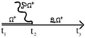
Let U(t,t1)=et1t𝑑t2Ω(t2)superscript𝑈𝑡subscript𝑡1superscript𝑒superscriptsubscriptsubscript𝑡1𝑡differential-dsubscript𝑡2superscriptΩsubscript𝑡2U^{\dagger}(t,t_{1})=e^{\int_{t_{1}}^{t}dt_{2}\Omega^{\dagger}(t_{2})} be the propagator appearing in gGK (Eq. 19), associated with the full dynamics ΩsuperscriptΩ\Omega^{\dagger}. We split Usuperscript𝑈U^{\dagger} into a part U1(t,t1)et1t𝑑t1Q1Ω(t1)superscriptsubscript𝑈1𝑡subscript𝑡1superscript𝑒superscriptsubscriptsubscript𝑡1𝑡differential-dsubscript𝑡1subscript𝑄1superscriptΩsubscript𝑡1U_{1}^{\dagger}(t,t_{1})\equiv e^{\int_{t_{1}}^{t}dt_{1}Q_{1}\Omega^{\dagger}(t_{1})} that evolves purely orthogonally to P1subscript𝑃1P_{1} and a part that interacts at least once with P1subscript𝑃1P_{1} (the notation t2subscript𝑡2t_{2} referring to the time of the last interaction, see Fig. 1), viz.

U(t,t1)=t1t𝑑t2U(t2,t1)P1Ω(t2)U1(t,t2)+U1(t,t1).superscript𝑈𝑡subscript𝑡1superscriptsubscriptsubscript𝑡1𝑡differential-dsubscript𝑡2superscript𝑈subscript𝑡2subscript𝑡1subscript𝑃1superscriptΩsubscript𝑡2superscriptsubscript𝑈1𝑡subscript𝑡2superscriptsubscript𝑈1𝑡subscript𝑡1U^{\dagger}(t,t_{1})=\int_{t_{1}}^{t}dt_{2}U^{\dagger}(t_{2},t_{1})P_{1}\Omega^{\dagger}(t_{2})U_{1}^{\dagger}(t,t_{2})+U_{1}^{\dagger}(t,t_{1}). (20)
Refer to caption
Figure 1: Schematic diagram of the decomposition of the full propagator U(t,t1)superscript𝑈𝑡subscript𝑡1U^{\dagger}(t,t_{1}), associated with the operator ΩsuperscriptΩ\Omega^{\dagger}, as performed in Eq. 20.

Inserting the decomposition of Eq. 20 into gGK (Eq. 19), we arrive at:

gtg0subscriptdelimited-⟨⟩𝑔𝑡subscriptdelimited-⟨⟩𝑔0\displaystyle\left\langle g\right\rangle_{t}-\left\langle g\right\rangle_{0} =\displaystyle= 0t𝑑t1Ω(t1)U(t,t1)g0superscriptsubscript0𝑡differential-dsubscript𝑡1subscriptdelimited-⟨⟩superscriptΩsubscript𝑡1superscript𝑈𝑡subscript𝑡1𝑔0\displaystyle\int_{0}^{t}dt_{1}\left\langle\Omega^{\dagger}(t_{1})U^{\dagger}(t,t_{1})g\right\rangle_{0} (21)
=\displaystyle= 0t𝑑t20t1𝑑t1Ω(t1)U(t2,t1)P1Ω(t2)U1(t,t2)g0superscriptsubscript0𝑡differential-dsubscript𝑡2superscriptsubscript0subscript𝑡1differential-dsubscript𝑡1subscriptdelimited-⟨⟩superscriptΩsubscript𝑡1superscript𝑈subscript𝑡2subscript𝑡1subscript𝑃1superscriptΩsubscript𝑡2superscriptsubscript𝑈1𝑡subscript𝑡2𝑔0\displaystyle\int_{0}^{t}dt_{2}\int_{0}^{t_{1}}dt_{1}\left\langle\Omega^{\dagger}(t_{1})U^{\dagger}(t_{2},t_{1})P_{1}\Omega^{\dagger}(t_{2})U_{1}^{\dagger}(t,t_{2})g\right\rangle_{0}
+0t𝑑t1Ω(t1)U1(t,t1)g0superscriptsubscript0𝑡differential-dsubscript𝑡1subscriptdelimited-⟨⟩superscriptΩsubscript𝑡1superscriptsubscript𝑈1𝑡subscript𝑡1𝑔0\displaystyle+\int_{0}^{t}dt_{1}\left\langle\Omega^{\dagger}(t_{1})U_{1}^{\dagger}(t,t_{1})g\right\rangle_{0}
=\displaystyle= 0t𝑑t2𝒒0t2𝑑t1Ω(t1)U(t2,t1)ρ𝒒0ρ𝒒t2ρ𝒒0ρ𝒒Ω(t2)U1(t,t2)gNS𝒒superscriptsubscript0𝑡differential-dsubscript𝑡2subscript𝒒subscriptdelimited-⟨⟩subscript𝜌𝒒subscript𝑡2subscriptdelimited-⟨⟩subscript𝜌𝒒0superscriptsubscript0subscript𝑡2differential-dsubscript𝑡1subscriptdelimited-⟨⟩superscriptΩsubscript𝑡1superscript𝑈subscript𝑡2subscript𝑡1subscript𝜌𝒒0delimited-⟨⟩superscriptsubscript𝜌𝒒superscriptΩsubscript𝑡2superscriptsubscript𝑈1𝑡subscript𝑡2𝑔𝑁subscript𝑆𝒒\displaystyle\int_{0}^{t}dt_{2}\sum_{\boldsymbol{q}}\underset{\left\langle\rho_{\boldsymbol{q}}\right\rangle_{t_{2}}-\left\langle\rho_{\boldsymbol{q}}\right\rangle_{0}}{\underbrace{\int_{0}^{t_{2}}dt_{1}\left\langle\Omega^{\dagger}(t_{1})U^{\dagger}(t_{2},t_{1})\rho_{\boldsymbol{q}}\right\rangle_{0}}}\frac{\left\langle\rho_{\boldsymbol{q}}^{\star}\Omega^{\dagger}(t_{2})U_{1}^{\dagger}(t,t_{2})g\right\rangle}{NS_{\boldsymbol{q}}}
+0t𝑑t1Ω(t1)U1(t,t1)g0(Orth1)subscriptOrth1superscriptsubscript0𝑡differential-dsubscript𝑡1subscriptdelimited-⟨⟩superscriptΩsubscript𝑡1superscriptsubscript𝑈1𝑡subscript𝑡1𝑔0\displaystyle+\underset{\mathrm{(Orth_{1})}}{\underbrace{\int_{0}^{t}dt_{1}\left\langle\Omega^{\dagger}(t_{1})U_{1}^{\dagger}(t,t_{1})g\right\rangle_{0}}}

where we have made use of gGK (applied to density fluctuations, gρ𝒒𝑔subscript𝜌𝒒g\to\rho_{\boldsymbol{q}}) in the last equality to reduce the first brace to ρ𝒒t2ρ𝒒0subscriptdelimited-⟨⟩subscript𝜌𝒒subscript𝑡2subscriptdelimited-⟨⟩subscript𝜌𝒒0\left\langle\rho_{\boldsymbol{q}}\right\rangle_{t_{2}}-\left\langle\rho_{\boldsymbol{q}}\right\rangle_{0}. One thus arrives at:

gtg0=0t𝑑t2𝒒(ρ𝒒t2ρ𝒒0)ρ𝒒Ω(t2)U1(t,t2)gNS𝒒+(Orth1).subscriptdelimited-⟨⟩𝑔𝑡subscriptdelimited-⟨⟩𝑔0superscriptsubscript0𝑡differential-dsubscript𝑡2subscript𝒒subscriptdelimited-⟨⟩subscript𝜌𝒒subscript𝑡2subscriptdelimited-⟨⟩subscript𝜌𝒒0delimited-⟨⟩superscriptsubscript𝜌𝒒superscriptΩsubscript𝑡2superscriptsubscript𝑈1𝑡subscript𝑡2𝑔𝑁subscript𝑆𝒒subscriptOrth1\left\langle g\right\rangle_{t}-\left\langle g\right\rangle_{0}=\int_{0}^{t}dt_{2}\sum_{\boldsymbol{q}}\left(\left\langle\rho_{\boldsymbol{q}}\right\rangle_{t_{2}}-\left\langle\rho_{\boldsymbol{q}}\right\rangle_{0}\right)\frac{\left\langle\rho_{\boldsymbol{q}}^{\star}\Omega^{\dagger}(t_{2})U_{1}^{\dagger}(t,t_{2})g\right\rangle}{NS_{\boldsymbol{q}}}+\mathrm{(Orth_{1})}. (22)

First, we focus on the dynamical correlator ρ𝒒Ω(t2)U1(t,t2)gdelimited-⟨⟩superscriptsubscript𝜌𝒒superscriptΩsubscript𝑡2superscriptsubscript𝑈1𝑡subscript𝑡2𝑔\left\langle\rho_{\boldsymbol{q}}^{\star}\Omega^{\dagger}(t_{2})U_{1}^{\dagger}(t,t_{2})g\right\rangle on the rhs and introduce the identity P1+Q1=1subscript𝑃1subscript𝑄11P_{1}+Q_{1}=1 as follows:

ρ𝒒Ω(t2)U1(t,t2)gNS𝒒delimited-⟨⟩superscriptsubscript𝜌𝒒superscriptΩsubscript𝑡2superscriptsubscript𝑈1𝑡subscript𝑡2𝑔𝑁subscript𝑆𝒒\displaystyle\frac{\left\langle\rho_{\boldsymbol{q}}^{\star}\Omega^{\dagger}(t_{2})U_{1}^{\dagger}(t,t_{2})g\right\rangle}{NS_{\boldsymbol{q}}} =\displaystyle= 1NS𝒒ρ𝒒Ω(t2)U1(t,t2)(P1+Q1)g1𝑁subscript𝑆𝒒delimited-⟨⟩superscriptsubscript𝜌𝒒superscriptΩsubscript𝑡2superscriptsubscript𝑈1𝑡subscript𝑡2subscript𝑃1subscript𝑄1𝑔\displaystyle\frac{1}{NS_{\boldsymbol{q}}}\left\langle\rho_{\boldsymbol{q}}^{\star}\Omega^{\dagger}(t_{2})U_{1}^{\dagger}(t,t_{2})\left(P_{1}+Q_{1}\right)g\right\rangle
=\displaystyle= 𝒌V𝒌gM𝒒𝒌(1)(t,t2)subscript𝒌superscriptsubscript𝑉𝒌𝑔superscriptsubscript𝑀𝒒𝒌1𝑡subscript𝑡2\displaystyle-\sum_{\boldsymbol{k}}V_{\boldsymbol{k}}^{g}M_{\boldsymbol{qk}}^{(1)}\left(t,t_{2}\right)
+1NS𝒒ρ𝒒Ω(t2)U1(t,t2)Q1g,1𝑁subscript𝑆𝒒delimited-⟨⟩superscriptsubscript𝜌𝒒superscriptΩsubscript𝑡2superscriptsubscript𝑈1𝑡subscript𝑡2subscript𝑄1𝑔\displaystyle+\frac{1}{NS_{\boldsymbol{q}}}\left\langle\rho_{\boldsymbol{q}}^{\star}\Omega^{\dagger}(t_{2})U_{1}^{\dagger}(t,t_{2})Q_{1}g\right\rangle,

where the vertex V𝒌gρ𝒌gNS𝒌superscriptsubscript𝑉𝒌𝑔delimited-⟨⟩superscriptsubscript𝜌𝒌𝑔𝑁subscript𝑆𝒌V_{\boldsymbol{k}}^{g}\equiv\frac{\left\langle\rho_{\boldsymbol{k}}^{\star}g\right\rangle}{NS_{\boldsymbol{k}}} quantifies the coupling of the observable g𝑔g to the density mode ρ𝒌subscript𝜌𝒌\rho_{\boldsymbol{k}} in the equilibrium distribution and

M𝒒𝒌(1)(t,t2)superscriptsubscript𝑀𝒒𝒌1𝑡subscript𝑡2\displaystyle M_{\boldsymbol{qk}}^{(1)}\left(t,t_{2}\right) \displaystyle\equiv ρ𝒒Ω(t2)U1(t,t2)ρ𝒌NS𝒒delimited-⟨⟩superscriptsubscript𝜌𝒒superscriptΩsubscript𝑡2superscriptsubscript𝑈1𝑡subscript𝑡2subscript𝜌𝒌𝑁subscript𝑆𝒒\displaystyle-\frac{\left\langle\rho_{\boldsymbol{q}}^{\star}\Omega^{\dagger}(t_{2})U_{1}^{\dagger}(t,t_{2})\rho_{\boldsymbol{k}}\right\rangle}{NS_{\boldsymbol{q}}}
=\displaystyle= 1NS𝒒[ρ𝒒j𝒗solv(𝒓j,t2)𝑭j\displaystyle\frac{1}{NS_{\boldsymbol{q}}}\Big{\langle}\Big{[}\rho_{\boldsymbol{q}}^{\star}\sum_{j}\boldsymbol{v}^{\mathrm{solv}}(\boldsymbol{r}_{j},t_{2})\cdot\boldsymbol{F}_{j}
+i𝒒(𝑭^𝒒+𝒗^𝒒(t2))]U1(t,t2)ρ𝒌\displaystyle\,\,\,\,+i\boldsymbol{q}\cdot\left(-\boldsymbol{\hat{F}_{q}}^{\star}+\boldsymbol{\hat{v}_{q}}^{\star}(t_{2})\right)\Big{]}U_{1}^{\dagger}(t,t_{2})\rho_{\boldsymbol{k}}\Big{\rangle}

is a memory kernel evaluated in the equilibrium distribution, with

𝑭^𝒒j𝑭jei𝒒𝒓j and 𝒗^𝒒(t)j𝒗solv(𝒓j,t)ei𝒒𝒓j.subscriptbold-^𝑭𝒒subscript𝑗subscript𝑭𝑗superscript𝑒𝑖𝒒subscript𝒓𝑗 and subscriptbold-^𝒗𝒒𝑡subscript𝑗superscript𝒗solvsubscript𝒓𝑗𝑡superscript𝑒𝑖𝒒subscript𝒓𝑗\boldsymbol{\hat{F}_{q}}\equiv\sum_{j}\boldsymbol{F}_{j}e^{-i\boldsymbol{q}\cdot\boldsymbol{r}_{j}}\text{ and }\boldsymbol{\hat{v}_{q}}(t)\equiv\sum_{j}\boldsymbol{v}^{\mathrm{solv}}(\boldsymbol{r}_{j},t)e^{-i\boldsymbol{q}\cdot\boldsymbol{r}_{j}}. (24)

3.4 Application to the density observable

Before turning to our main interest, i.e., the stress, we wish to illustrate the principle of the projection scheme for a generic flow, but on a simpler observable, namely, the density g=ρ𝒑,𝒑dformulae-sequence𝑔subscript𝜌𝒑𝒑superscript𝑑g=\rho_{\boldsymbol{p}},\,\boldsymbol{p}\in\mathbb{R}^{d}, for which the complement Q1gsubscript𝑄1𝑔Q_{1}g vanishes by definition. The following calculations need not be performed in the homogeneous auxiliary frame; they hold true for an inhomogeneous flow.

Applying Eq. 22 to density modes (V𝒌ρ𝒑ρ𝒌ρ𝒑NS𝒌=δ𝒌,𝒑superscriptsubscript𝑉𝒌subscript𝜌𝒑delimited-⟨⟩superscriptsubscript𝜌𝒌subscript𝜌𝒑𝑁subscript𝑆𝒌subscript𝛿𝒌𝒑V_{\boldsymbol{k}}^{\rho_{\boldsymbol{p}}}\equiv\frac{\left\langle\rho_{\boldsymbol{k}}^{\star}\rho_{\boldsymbol{p}}\right\rangle}{NS_{\boldsymbol{k}}}=\delta_{\boldsymbol{k},\boldsymbol{p}}) leads to

ρ𝒑tρ𝒑0subscriptdelimited-⟨⟩subscript𝜌𝒑𝑡subscriptdelimited-⟨⟩subscript𝜌𝒑0\displaystyle\left\langle\rho_{\boldsymbol{p}}\right\rangle_{t}-\left\langle\rho_{\boldsymbol{p}}\right\rangle_{0} =\displaystyle= 0t𝑑t1𝒒[ρ𝒒t1ρ𝒒0]M𝒒𝒑(1)(t,t1)+(Orth1),superscriptsubscript0𝑡differential-dsubscript𝑡1subscript𝒒delimited-[]subscriptdelimited-⟨⟩subscript𝜌𝒒subscript𝑡1subscriptdelimited-⟨⟩subscript𝜌𝒒0superscriptsubscript𝑀𝒒𝒑1𝑡subscript𝑡1Orth1\displaystyle-\int_{0}^{t}dt_{1}\sum_{\boldsymbol{q}}\left[\left\langle\rho_{\boldsymbol{q}}\right\rangle_{t_{1}}-\left\langle\rho_{\boldsymbol{q}}\right\rangle_{0}\right]M_{\boldsymbol{qp}}^{(1)}\left(t,t_{1}\right)+(\mathrm{Orth}1),

where M𝒒𝒑(1)(t,t1)superscriptsubscript𝑀𝒒𝒑1𝑡subscript𝑡1M_{\boldsymbol{qp}}^{(1)}\left(t,t_{1}\right) is given in Eq. 3.3 and (Orth1)0t𝑑t1Ω(t1)U1(t,t1)ρ𝒑0Orth1superscriptsubscript0𝑡differential-dsubscript𝑡1subscriptdelimited-⟨⟩superscriptΩsubscript𝑡1superscriptsubscript𝑈1𝑡subscript𝑡1subscript𝜌𝒑0(\mathrm{Orth}1)\equiv\int_{0}^{t}dt_{1}\left\langle\Omega^{\dagger}(t_{1})U_{1}^{\dagger}(t,t_{1})\rho_{\boldsymbol{p}}\right\rangle_{0}.

Taking a derivative with respect to time t𝑡t yields

tρ𝒑tsubscript𝑡subscriptdelimited-⟨⟩subscript𝜌𝒑𝑡\displaystyle\partial_{t}\left\langle\rho_{\boldsymbol{p}}\right\rangle_{t} =\displaystyle= 𝒒[ρ𝒒tρ𝒒0]M𝒒𝒑(1)(t,t)subscript𝒒delimited-[]subscriptdelimited-⟨⟩subscript𝜌𝒒𝑡subscriptdelimited-⟨⟩subscript𝜌𝒒0superscriptsubscript𝑀𝒒𝒑1𝑡𝑡\displaystyle-\sum_{\boldsymbol{q}}\left[\left\langle\rho_{\boldsymbol{q}}\right\rangle_{t}-\left\langle\rho_{\boldsymbol{q}}\right\rangle_{0}\right]M_{\boldsymbol{qp}}^{(1)}\left(t,t\right) (25)
0t𝑑t1𝒒[ρ𝒒t1ρ𝒒0]tM𝒒𝒑(1)(t,t1)+S^𝒑(t).superscriptsubscript0𝑡differential-dsubscript𝑡1subscript𝒒delimited-[]subscriptdelimited-⟨⟩subscript𝜌𝒒subscript𝑡1subscriptdelimited-⟨⟩subscript𝜌𝒒0subscript𝑡superscriptsubscript𝑀𝒒𝒑1𝑡subscript𝑡1subscript^𝑆𝒑𝑡\displaystyle\>\>\>\>-\int_{0}^{t}dt_{1}\sum_{\boldsymbol{q}}\left[\left\langle\rho_{\boldsymbol{q}}\right\rangle_{t_{1}}-\left\langle\rho_{\boldsymbol{q}}\right\rangle_{0}\right]\partial_{t}M_{\boldsymbol{qp}}^{(1)}(t,t_{1})+\hat{S}_{\boldsymbol{p}}(t).

Here, we have used the explicit notation S^𝒑(t)subscript^𝑆𝒑𝑡\hat{S}_{\boldsymbol{p}}(t) for t(Orth1)subscript𝑡Orth1\partial_{t}\mathrm{(Orth1)};

S^𝒑(t)=i𝒑𝑭^𝒑+𝒗^𝒑i𝒑ρ𝒑00t𝑑t1Ω(t1)U1(t,t1)Q1i𝒑(𝑭^𝒑+𝒗^𝒑)0.subscript^𝑆𝒑𝑡𝑖𝒑subscriptdelimited-⟨⟩subscriptbold-^𝑭𝒑subscriptbold-^𝒗𝒑𝑖𝒑subscript𝜌𝒑0superscriptsubscript0𝑡differential-dsubscript𝑡1subscriptdelimited-⟨⟩superscriptΩsubscript𝑡1superscriptsubscript𝑈1𝑡subscript𝑡1subscript𝑄1𝑖𝒑subscriptbold-^𝑭𝒑subscriptbold-^𝒗𝒑0\hat{S}_{\boldsymbol{p}}(t)=-i\boldsymbol{p}\cdot\langle\boldsymbol{\hat{F}_{p}}+\boldsymbol{\hat{v}_{p}}-i\boldsymbol{p}\rho_{\boldsymbol{p}}\rangle_{0}-\int_{0}^{t}dt_{1}\langle\Omega^{\dagger}(t_{1})U_{1}^{\dagger}(t,t_{1})Q_{1}i\boldsymbol{p}\cdot(\boldsymbol{\hat{F}_{p}}+\boldsymbol{\hat{v}_{p}})\rangle_{0}. (26)

The term M𝒒𝒑(1)(t,t)=(NS𝒒)1ρ𝒒Ω(t)ρ𝒑superscriptsubscript𝑀𝒒𝒑1𝑡𝑡superscript𝑁subscript𝑆𝒒1delimited-⟨⟩superscriptsubscript𝜌𝒒superscriptΩ𝑡subscript𝜌𝒑M_{\boldsymbol{qp}}^{(1)}\left(t,t\right)=-\left(NS_{\boldsymbol{q}}\right)^{-1}\left\langle\rho_{\boldsymbol{q}}^{\star}\Omega^{\dagger}(t)\rho_{\boldsymbol{p}}\right\rangle can be simplified. Using the equilibrium (i.e., 𝒗solv=𝟎superscript𝒗solv0\boldsymbol{v}^{\mathrm{solv}}=\boldsymbol{0}) Smoluchowski operator ΩeqsuperscriptsubscriptΩeq\Omega_{\mathrm{eq}}^{\dagger} from Eq. 16, we can write

ρ𝒒Ω(t)ρ𝒑delimited-⟨⟩superscriptsubscript𝜌𝒒superscriptΩ𝑡subscript𝜌𝒑\displaystyle\left\langle\rho_{\boldsymbol{q}}^{\star}\Omega^{\dagger}(t)\rho_{\boldsymbol{p}}\right\rangle =\displaystyle= ρ𝒒Ωeqρ𝒑+ρ𝒒j𝒗solv(𝒓𝒋,t)jρ𝒑,delimited-⟨⟩superscriptsubscript𝜌𝒒superscriptsubscriptΩeqsubscript𝜌𝒑delimited-⟨⟩superscriptsubscript𝜌𝒒subscript𝑗superscript𝒗solvsubscript𝒓𝒋𝑡subscript𝑗subscript𝜌𝒑\displaystyle\left\langle\rho_{\boldsymbol{q}}^{\star}\Omega_{\mathrm{eq}}^{\dagger}\rho_{\boldsymbol{p}}\right\rangle+\left\langle\rho_{\boldsymbol{q}}^{\star}\sum_{j}\boldsymbol{v}^{\mathrm{solv}}\left(\boldsymbol{r_{j}},t\right)\cdot\partial_{j}\rho_{\boldsymbol{p}}\right\rangle,

where, using partial integration,

ρ𝒒Ωeqρ𝒑delimited-⟨⟩superscriptsubscript𝜌𝒒superscriptsubscriptΩeqsubscript𝜌𝒑\displaystyle\left\langle\rho_{\boldsymbol{q}}^{\star}\Omega_{\mathrm{eq}}^{\dagger}\rho_{\boldsymbol{p}}\right\rangle =\displaystyle= ρ𝒒j(j+𝑭𝒋)jρ𝒑delimited-⟨⟩superscriptsubscript𝜌𝒒subscript𝑗subscript𝑗subscript𝑭𝒋subscript𝑗subscript𝜌𝒑\displaystyle\left\langle\rho_{\boldsymbol{q}}^{\star}\sum_{j}\left(\partial_{j}+\boldsymbol{F_{j}}\right)\cdot\partial_{j}\rho_{\boldsymbol{p}}\right\rangle
=\displaystyle= 𝑑Γψeq(Γ)ρ𝒒j(j+𝑭𝒋)jρ𝒑differential-dΓsubscript𝜓eqΓsuperscriptsubscript𝜌𝒒subscript𝑗subscript𝑗subscript𝑭𝒋subscript𝑗subscript𝜌𝒑\displaystyle\int d\Gamma\psi_{\mathrm{eq}}(\Gamma)\rho_{\boldsymbol{q}}^{\star}\sum_{j}\left(\partial_{j}+\boldsymbol{F_{j}}\right)\cdot\partial_{j}\rho_{\boldsymbol{p}}
=\displaystyle= 𝑑Γj{j[ψeq(Γ)ρ𝒒]ρ𝒒j𝑭𝒋ψeq(Γ)}jρ𝒑differential-dΓsubscript𝑗subscript𝑗delimited-[]subscript𝜓eqΓsuperscriptsubscript𝜌𝒒superscriptsubscript𝜌𝒒subscript𝑗subscript𝑭𝒋subscript𝜓eqΓsubscript𝑗subscript𝜌𝒑\displaystyle-\int d\Gamma\sum_{j}\left\{\partial_{j}\left[\psi_{\mathrm{eq}}(\Gamma)\rho_{\boldsymbol{q}}^{\star}\right]-\rho_{\boldsymbol{q}}^{\star}\sum_{j}\boldsymbol{F_{j}}\psi_{\mathrm{eq}}(\Gamma)\right\}\cdot\partial_{j}\rho_{\boldsymbol{p}}
=\displaystyle= 𝒒𝒑jei(𝒒𝒑)𝒓𝒋𝒒𝒑delimited-⟨⟩subscript𝑗superscript𝑒𝑖𝒒𝒑subscript𝒓𝒋\displaystyle-\boldsymbol{q}\cdot\boldsymbol{p}\left\langle\sum_{j}e^{i(\boldsymbol{q}-\boldsymbol{p})\cdot\boldsymbol{r_{j}}}\right\rangle
=\displaystyle= 𝒑2δ𝒒𝒑N.superscript𝒑2subscript𝛿𝒒𝒑𝑁\displaystyle-\boldsymbol{p}^{2}\delta_{\boldsymbol{qp}}N.

The second term, ρ𝒒j𝒗solv(𝒓𝒋,t)jρ𝒑F𝒒𝒑delimited-⟨⟩superscriptsubscript𝜌𝒒subscript𝑗superscript𝒗solvsubscript𝒓𝒋𝑡subscript𝑗subscript𝜌𝒑subscript𝐹𝒒𝒑\left\langle\rho_{\boldsymbol{q}}^{\star}\sum_{j}\boldsymbol{v}^{\mathrm{solv}}\left(\boldsymbol{r_{j}},t\right)\cdot\partial_{j}\rho_{\boldsymbol{p}}\right\rangle\equiv F_{\boldsymbol{qp}}, is most easily simplified by first backward-Fourier transforming it with respect to 𝐩𝐩\boldsymbol{p} only, viz.,

F𝒒(𝒓0)subscript𝐹𝒒subscript𝒓0\displaystyle F_{\boldsymbol{q}}\left(\boldsymbol{r}_{0}\right) =\displaystyle= ρ𝒒j𝒗solv(𝒓𝒋,t)jρ(𝒓0),delimited-⟨⟩superscriptsubscript𝜌𝒒subscript𝑗superscript𝒗solvsubscript𝒓𝒋𝑡subscript𝑗𝜌subscript𝒓0\displaystyle\left\langle\rho_{\boldsymbol{q}}^{\star}\sum_{j}\boldsymbol{v}^{\mathrm{solv}}\left(\boldsymbol{r_{j}},t\right)\cdot\partial_{j}\rho\left(\boldsymbol{r}_{0}\right)\right\rangle,
=\displaystyle= ρ𝒒j𝒗solv(𝒓𝒋,t)𝒓0δ(𝒓0𝒓𝒋).delimited-⟨⟩superscriptsubscript𝜌𝒒subscript𝑗superscript𝒗solvsubscript𝒓𝒋𝑡subscriptsubscript𝒓0𝛿subscript𝒓0subscript𝒓𝒋\displaystyle-\left\langle\rho_{\boldsymbol{q}}^{\star}\sum_{j}\boldsymbol{v}^{\mathrm{solv}}\left(\boldsymbol{r_{j}},t\right)\cdot\partial_{\boldsymbol{r}_{0}}\delta\left(\boldsymbol{r}_{0}-\boldsymbol{r_{j}}\right)\right\rangle.
=\displaystyle= 𝒓0ρ𝒒j𝒗solv(𝒓𝒋,t)δ(𝒓0𝒓𝒋)subscriptsubscript𝒓0delimited-⟨⟩superscriptsubscript𝜌𝒒subscript𝑗superscript𝒗solvsubscript𝒓𝒋𝑡𝛿subscript𝒓0subscript𝒓𝒋\displaystyle-\partial_{\boldsymbol{r}_{0}}\cdot\left\langle\rho_{\boldsymbol{q}}^{\star}\sum_{j}\boldsymbol{v}^{\mathrm{solv}}\left(\boldsymbol{r_{j}},t\right)\delta\left(\boldsymbol{r}_{0}-\boldsymbol{r_{j}}\right)\right\rangle
=\displaystyle= ρ𝒒𝒗solv(𝒓0,t)𝒓0ρ(𝒓0),delimited-⟨⟩superscriptsubscript𝜌𝒒superscript𝒗solvsubscript𝒓0𝑡subscriptsubscript𝒓0𝜌subscript𝒓0\displaystyle-\left\langle\rho_{\boldsymbol{q}}^{\star}\boldsymbol{v}^{\mathrm{solv}}\left(\boldsymbol{r}_{0},t\right)\cdot\partial_{\boldsymbol{r}_{0}}\rho\left(\boldsymbol{r}_{0}\right)\right\rangle,

where we have used the incompressibility of the velocity field, viz., 𝒓0𝒗solv(𝒓0,t)=0subscriptsubscript𝒓0superscript𝒗solvsubscript𝒓0𝑡0\partial_{\boldsymbol{r}_{0}}\cdot\boldsymbol{v}^{\mathrm{solv}}\left(\boldsymbol{r}_{0},t\right)=0. It suffices to transform F𝒒(𝒓0)subscript𝐹𝒒subscript𝒓0F_{\boldsymbol{q}}\left(\boldsymbol{r}_{0}\right) back into reciprocal space (with respect to 𝒓0subscript𝒓0\boldsymbol{r}_{0}) to obtain:

F𝒒𝒑subscript𝐹𝒒𝒑\displaystyle F_{\boldsymbol{qp}} =\displaystyle= 𝒌ρ𝒒𝒗𝒌(t)i(𝒑𝒌)ρ𝒑𝒌subscript𝒌delimited-⟨⟩superscriptsubscript𝜌𝒒subscript𝒗𝒌𝑡𝑖𝒑𝒌subscript𝜌𝒑𝒌\displaystyle-\sum_{\boldsymbol{k}}\left\langle\rho_{\boldsymbol{q}}^{\star}\boldsymbol{v}_{\boldsymbol{k}}(t)\cdot i\left(\boldsymbol{p}-\boldsymbol{k}\right)\rho_{\boldsymbol{p}-\boldsymbol{k}}\right\rangle
=\displaystyle= 𝒗𝒌(t)i𝒒ρ𝒒ρ𝒒subscript𝒗𝒌𝑡𝑖𝒒delimited-⟨⟩superscriptsubscript𝜌𝒒subscript𝜌𝒒\displaystyle-\boldsymbol{v}_{\boldsymbol{k}}(t)\cdot i\boldsymbol{q}\left\langle\rho_{\boldsymbol{q}}^{\star}\rho_{\boldsymbol{q}}\right\rangle
=\displaystyle= iN𝒗𝒑𝒒solv(t)𝒒S𝒒.𝑖𝑁superscriptsubscript𝒗𝒑𝒒solv𝑡𝒒subscript𝑆𝒒\displaystyle-iN\boldsymbol{v}_{\boldsymbol{p}-\boldsymbol{q}}^{\mathrm{solv}}\left(t\right)\cdot\boldsymbol{q}S_{\boldsymbol{q}}.

Collecting these contributions into Eq. 25, one arrives at an equation of evolution of density fluctuations:

tρ𝒑t+𝒒𝒗𝒑𝒒solv(t)i𝒒ρ𝒒tsubscript𝑡subscriptdelimited-⟨⟩subscript𝜌𝒑𝑡subscript𝒒superscriptsubscript𝒗𝒑𝒒solv𝑡𝑖𝒒subscriptdelimited-⟨⟩subscript𝜌𝒒𝑡\displaystyle\partial_{t}\left\langle\rho_{\boldsymbol{p}}\right\rangle_{t}+\sum_{\boldsymbol{q}}\boldsymbol{v}_{\boldsymbol{p}-\boldsymbol{q}}^{\mathrm{solv}}\left(t\right)\cdot i\boldsymbol{q}\left\langle\rho_{\boldsymbol{q}}\right\rangle_{t} =\displaystyle= 𝒑2S𝒑ρ𝒑t𝒒0t𝑑t1tM𝒒𝒑(1)(t,t1)ρ𝒒t1superscript𝒑2subscript𝑆𝒑subscriptdelimited-⟨⟩subscript𝜌𝒑𝑡subscript𝒒superscriptsubscript0𝑡differential-dsubscript𝑡1subscript𝑡superscriptsubscript𝑀𝒒𝒑1𝑡subscript𝑡1subscriptdelimited-⟨⟩subscript𝜌𝒒subscript𝑡1\displaystyle-\frac{\boldsymbol{p}^{2}}{S_{\boldsymbol{p}}}\left\langle\rho_{\boldsymbol{p}}\right\rangle_{t}-\sum_{\boldsymbol{q}}\int_{0}^{t}dt_{1}\partial_{t}M_{\boldsymbol{qp}}^{(1)}\left(t,t_{1}\right)\left\langle\rho_{\boldsymbol{q}}\right\rangle_{t_{1}} (27)
+S^𝒑(t).subscript^𝑆𝒑𝑡\displaystyle\>\>\>\>\>\>\>\>\>\>\>\>\>\>\>+\hat{S}_{\boldsymbol{p}}(t).

Let us emphasise the physical meaning of the different terms:

(i) the second term on the lhs is the advection term established in Section 2.2;

(ii) the first one on the rhs permits the relaxation of fluctuations through diffusion. Note that the normalising factor S𝒑1superscriptsubscript𝑆𝒑1S_{\boldsymbol{p}}^{-1} is expected, because the relaxation of a density mode ρ𝒑subscript𝜌𝒑\rho_{\boldsymbol{p}} does not require single-particle diffusion over a lengthscale 𝒑1superscriptnorm𝒑1\left\|\boldsymbol{p}\right\|^{-1}! Besides, if the density field is smoothed via coarse-graining (i.e., ρ𝒑ρ𝒑ϕ𝒑subscript𝜌𝒑subscript𝜌𝒑subscriptitalic-ϕ𝒑\rho_{\boldsymbol{p}}\rightarrow\rho_{\boldsymbol{p}}\phi_{\boldsymbol{p}}, with ϕ𝒑subscriptitalic-ϕ𝒑\phi_{\boldsymbol{p}} akin to a Gaussian of half-width a few particle diameters), the fast relaxational modes at high 𝒑𝒑\boldsymbol{p} are suppressed, and the normalising factor then tends to S𝟎1superscriptsubscript𝑆01S_{\boldsymbol{0}}^{-1}, which is directly related to the compressibility of the suspension.

(iii) The second term on the rhs reflects the evolution in orthogonal space of the density fluctuations created in the past and their final coupling back to present fluctuations.

(iv) S^𝐩(t)subscript^𝑆𝐩𝑡\hat{S}_{\boldsymbol{p}}(t) is a source term that results from interactions with nonlinear density modes. Consistently with the expectation that density heterogeneities in an incompressible flow are due to collective effects, e.g., stress equilibration, it is the only term that can potentially create density inhomogeneities, insofar as the other terms are associated to pre-existing density heterogeneities. If a homogeneous flow is imposed to an initally uniform system, translational invariance imposes that, for finite 𝒑𝒑\boldsymbol{p}, 𝑭^𝒑0=0subscriptdelimited-⟨⟩subscriptbold-^𝑭𝒑00\left\langle\boldsymbol{\hat{F}_{p}}\right\rangle_{0}=0, 𝝆𝒑0=0subscriptdelimited-⟨⟩subscript𝝆𝒑00\left\langle\boldsymbol{\rho_{p}}\right\rangle_{0}=0, i𝒑𝒗^𝒑0=0𝑖𝒑subscriptdelimited-⟨⟩subscriptbold-^𝒗𝒑00i\boldsymbol{p}\cdot\left\langle\boldsymbol{\hat{v}_{p}}\right\rangle_{0}=0 in Eq. 26, ergo S^𝒑(t)=0subscript^𝑆𝒑𝑡0\hat{S}_{\boldsymbol{p}}(t)=0 at all times, for all 𝒑𝒑\boldsymbol{p}; as expected, the source term then vanishes.

Finally, by comparing Eq. 27 to the mass conservation equation,

tρ𝒑t+i𝒑𝒋𝒑collt=0,subscript𝑡subscriptdelimited-⟨⟩subscript𝜌𝒑𝑡𝑖𝒑subscriptdelimited-⟨⟩subscriptsuperscript𝒋coll𝒑𝑡0\partial_{t}\langle\rho_{\boldsymbol{p}}\rangle_{t}+i\boldsymbol{p}\cdot\langle\boldsymbol{j}^{\mathrm{coll}}_{\boldsymbol{p}}\rangle_{t}=0,

where 𝒋𝒑collj=1N𝒓˙𝒋ei𝒑𝒓𝒋subscriptsuperscript𝒋coll𝒑superscriptsubscript𝑗1𝑁subscriptbold-˙𝒓𝒋superscript𝑒𝑖𝒑subscript𝒓𝒋\boldsymbol{j}^{\mathrm{coll}}_{\boldsymbol{p}}\equiv\sum_{j=1}^{N}\boldsymbol{\dot{r}_{j}}e^{-i\boldsymbol{p}\cdot\boldsymbol{r_{j}}} is the colloidal flux, it can be seen that, in a heterogeneous flow, the colloidal velocity 𝒖coll(𝒓,t)𝒋coll(𝒓)tρ(𝒓)tsuperscript𝒖coll𝒓𝑡subscriptdelimited-⟨⟩superscript𝒋coll𝒓𝑡subscriptdelimited-⟨⟩𝜌𝒓𝑡\boldsymbol{u}^{\mathrm{coll}}(\boldsymbol{r},t)\equiv\frac{\langle\boldsymbol{j}^{\mathrm{coll}}(\boldsymbol{r})\rangle_{t}}{\langle\rho(\boldsymbol{r})\rangle_{t}} will generally differ from the driving solvent velocity 𝒗solv(𝒓,t)superscript𝒗solv𝒓𝑡\boldsymbol{v}^{\mathrm{solv}}(\boldsymbol{r},t).

3.5 Orthogonal dynamics

Let us come back to a generic observable g𝑔g and refine the description of term (Orth1) in Eq. 21. In principle, the propagator decomposition of Eq. 20 can be iterated, and the propagator U1superscriptsubscript𝑈1U_{1}^{\dagger}, split into a part evolving with P2Q1Ωsubscript𝑃2subscript𝑄1superscriptΩP_{2}Q_{1}\Omega^{\dagger} and an orthogonal part U2superscriptsubscript𝑈2U_{2}^{\dagger}, and so on, ad libitum. Schematically, one would then get

gtsubscriptdelimited-⟨⟩𝑔𝑡\displaystyle\left\langle g\right\rangle_{t} \displaystyle\approx g00t𝑑t2𝒒,𝒌(ρ𝒒t2ρ𝒒0)V1()M𝒒𝒌(1)(t,t2)subscriptdelimited-⟨⟩𝑔0superscriptsubscript0𝑡differential-dsubscript𝑡2subscript𝒒𝒌subscriptdelimited-⟨⟩subscript𝜌𝒒subscript𝑡2subscriptdelimited-⟨⟩subscript𝜌𝒒0subscript𝑉1superscriptsubscript𝑀𝒒𝒌1𝑡subscript𝑡2\displaystyle\left\langle g\right\rangle_{0}-\int_{0}^{t}dt_{2}\sum_{\boldsymbol{q},\boldsymbol{k}}\left(\left\langle\rho_{\boldsymbol{q}}\right\rangle_{t_{2}}-\left\langle\rho_{\boldsymbol{q}}\right\rangle_{0}\right)V_{1}\left(\cdot\right)M_{\boldsymbol{qk}}^{(1)}\left(t,t_{2}\right)
0t𝑑t2𝒌,𝒑,𝒌,𝒑(ρ𝒌ρ𝒑t2ρ𝒌ρ𝒑0)V2()M𝒒𝒌𝒒𝒌(2)(t,t2)+,superscriptsubscript0𝑡differential-dsubscript𝑡2subscript𝒌𝒑superscript𝒌bold-′superscript𝒑bold-′subscriptdelimited-⟨⟩subscript𝜌𝒌subscript𝜌𝒑subscript𝑡2subscriptdelimited-⟨⟩subscript𝜌𝒌subscript𝜌𝒑0subscript𝑉2superscriptsubscript𝑀𝒒𝒌superscript𝒒bold-′superscript𝒌bold-′2𝑡subscript𝑡2\displaystyle-\int_{0}^{t}dt_{2}\sum_{\boldsymbol{k},\boldsymbol{p},\boldsymbol{k^{\prime}},\boldsymbol{p^{\prime}}}\left(\left\langle\rho_{\boldsymbol{k}}\rho_{\boldsymbol{p}}\right\rangle_{t_{2}}-\left\langle\rho_{\boldsymbol{k}}\rho_{\boldsymbol{p}}\right\rangle_{0}\right)V_{2}\left(\cdot\right)M_{\boldsymbol{qkq^{\prime}k^{\prime}}}^{(2)}(t,t_{2})+\ldots,

and the orthogonal evolutions denoted by M(n)(t,t2)superscript𝑀𝑛𝑡subscript𝑡2M^{(n)}(t,t_{2}) would then be constrained to smaller and smaller spaces. However, following Ref. [12], we adopt a more pragmatic approach by directly introducing the projector P2subscript𝑃2P_{2} in (Orth1), viz.,

(Orth1)subscriptOrth1\displaystyle\mathrm{(Orth_{1})} \displaystyle\equiv 0t𝑑t1Ω(t1)Q1U1(t,t1)g0superscriptsubscript0𝑡differential-dsubscript𝑡1subscriptdelimited-⟨⟩superscriptΩsubscript𝑡1subscript𝑄1superscriptsubscript𝑈1𝑡subscript𝑡1𝑔0\displaystyle\int_{0}^{t}dt_{1}\left\langle\Omega^{\dagger}(t_{1})Q_{1}U_{1}^{\dagger}(t,t_{1})g\right\rangle_{0} (29)
\displaystyle\approx 0t𝑑t1Ω(t1)Q1P2U1(t,t1)P2g0superscriptsubscript0𝑡differential-dsubscript𝑡1subscriptdelimited-⟨⟩superscriptΩsubscript𝑡1subscript𝑄1subscript𝑃2superscriptsubscript𝑈1𝑡subscript𝑡1subscript𝑃2𝑔0\displaystyle\int_{0}^{t}dt_{1}\left\langle\Omega^{\dagger}(t_{1})Q_{1}P_{2}U_{1}^{\dagger}(t,t_{1})P_{2}g\right\rangle_{0}
\displaystyle\approx 0t𝑑t1𝒌>𝒑𝒌>𝒑V0,𝒌,𝒑(t1)V𝒌,𝒑gρ𝒌ρ𝒑U1(t,t1)ρ𝒌ρ𝒑N2S𝒌S𝒑,superscriptsubscript0𝑡differential-dsubscript𝑡1superscript𝒌bold-′superscript𝒑bold-′subscript𝒌𝒑subscript𝑉0𝒌𝒑subscript𝑡1superscriptsubscript𝑉superscript𝒌bold-′superscript𝒑bold-′𝑔delimited-⟨⟩superscriptsubscript𝜌𝒌superscriptsubscript𝜌𝒑superscriptsubscript𝑈1𝑡subscript𝑡1subscript𝜌superscript𝒌bold-′subscript𝜌superscript𝒑bold-′superscript𝑁2subscript𝑆𝒌subscript𝑆𝒑\displaystyle\int_{0}^{t}dt_{1}\underset{{}_{\boldsymbol{k^{\prime}}>\boldsymbol{p^{\prime}}}}{\sum_{\boldsymbol{k}>\boldsymbol{p}}}V_{0,\boldsymbol{k},\boldsymbol{p}}\left(t_{1}\right)V_{\boldsymbol{k^{\prime}},\boldsymbol{p^{\prime}}}^{g}\frac{\left\langle\rho_{\boldsymbol{k}}^{\star}\rho_{\boldsymbol{p}}^{\star}U_{1}^{\dagger}(t,t_{1})\rho_{\boldsymbol{k^{\prime}}}\rho_{\boldsymbol{p^{\prime}}}\right\rangle}{N^{2}S_{\boldsymbol{k}}S_{\boldsymbol{p}}},

where

V0,𝒌,𝒑(t1)subscript𝑉0𝒌𝒑subscript𝑡1\displaystyle V_{0,\boldsymbol{k},\boldsymbol{p}}\left(t_{1}\right) \displaystyle\equiv Ω(t1)Q1ρ𝒌ρ𝒑0subscriptdelimited-⟨⟩superscriptΩsubscript𝑡1subscript𝑄1subscript𝜌𝒌subscript𝜌𝒑0\displaystyle\left\langle\Omega^{\dagger}(t_{1})Q_{1}\rho_{\boldsymbol{k}}\rho_{\boldsymbol{p}}\right\rangle_{0}
V𝒌,𝒑gsuperscriptsubscript𝑉superscript𝒌bold-′superscript𝒑bold-′𝑔\displaystyle V_{\boldsymbol{k^{\prime}},\boldsymbol{p^{\prime}}}^{g} \displaystyle\equiv ρ𝒌ρ𝒑gN2S𝒌S𝒑delimited-⟨⟩subscriptsuperscript𝜌superscript𝒌bold-′subscriptsuperscript𝜌superscript𝒑bold-′𝑔superscript𝑁2subscript𝑆superscript𝒌bold-′subscript𝑆superscript𝒑bold-′\displaystyle\frac{\left\langle\rho^{*}_{\boldsymbol{k^{\prime}}}\rho^{*}_{\boldsymbol{p^{\prime}}}g\right\rangle}{N^{2}S_{\boldsymbol{k^{\prime}}}S_{\boldsymbol{p^{\prime}}}}

are vertices that represent, respectively, the creation and relaxation of bilinear density modes with respect to the initial configuration and the coupling strength of the observable g𝑔g to these modes. If the initial configuration ψ0subscript𝜓0\psi_{0} and the velocity gradient at t1subscript𝑡1t_{1} are close to homogeneous, then V0,𝒌,𝒑(t1)subscript𝑉0𝒌𝒑subscript𝑡1V_{0,\boldsymbol{k},\boldsymbol{p}}\left(t_{1}\right) is nonzero only for 𝒑𝒌𝒑𝒌\boldsymbol{p}\approx-\boldsymbol{k}, and if g𝑔g is a spatial average, that is, if only small-wavenumber modes contribute to its Fourier decomposition, then V𝒌,𝒑gsuperscriptsubscript𝑉superscript𝒌bold-′superscript𝒑bold-′𝑔V_{\boldsymbol{k^{\prime}},\boldsymbol{p^{\prime}}}^{g} is nonzero only if 𝒑𝒌superscript𝒑bold-′superscript𝒌bold-′\boldsymbol{p^{\prime}}\approx-\boldsymbol{k^{\prime}}.

To conclude, the density-pair correlation function ρ𝒌ρ𝒑U1(t,t1)ρ𝒌ρ𝒑delimited-⟨⟩superscriptsubscript𝜌𝒌superscriptsubscript𝜌𝒑superscriptsubscript𝑈1𝑡subscript𝑡1subscript𝜌superscript𝒌bold-′subscript𝜌superscript𝒑bold-′\left\langle\rho_{\boldsymbol{k}}^{\star}\rho_{\boldsymbol{p}}^{\star}U_{1}^{\dagger}(t,t_{1})\rho_{\boldsymbol{k^{\prime}}}\rho_{\boldsymbol{p^{\prime}}}\right\rangle is approximated through Gaussian factoring, which is a central approximation of mode-coupling theory [21]:

ρ𝒌ρ𝒑U1(t,t1)ρ𝒌ρ𝒑N2S𝒌S𝒑delimited-⟨⟩superscriptsubscript𝜌𝒌superscriptsubscript𝜌𝒑superscriptsubscript𝑈1𝑡subscript𝑡1subscript𝜌superscript𝒌bold-′subscript𝜌superscript𝒑bold-′superscript𝑁2subscript𝑆𝒌subscript𝑆𝒑\displaystyle\frac{\left\langle\rho_{\boldsymbol{k}}^{\star}\rho_{\boldsymbol{p}}^{\star}U_{1}^{\dagger}(t,t_{1})\rho_{\boldsymbol{k^{\prime}}}\rho_{\boldsymbol{p^{\prime}}}\right\rangle}{N^{2}S_{\boldsymbol{k}}S_{\boldsymbol{p}}} \displaystyle\approx ρ𝒌ρ𝒑U(t,t1)ρ𝒌ρ𝒑N2S𝒌S𝒑delimited-⟨⟩superscriptsubscript𝜌𝒌superscriptsubscript𝜌𝒑superscript𝑈𝑡subscript𝑡1subscript𝜌superscript𝒌bold-′subscript𝜌superscript𝒑bold-′superscript𝑁2subscript𝑆𝒌subscript𝑆𝒑\displaystyle\frac{\left\langle\rho_{\boldsymbol{k}}^{\star}\rho_{\boldsymbol{p}}^{\star}U^{\dagger}(t,t_{1})\rho_{\boldsymbol{k^{\prime}}}\rho_{\boldsymbol{p^{\prime}}}\right\rangle}{N^{2}S_{\boldsymbol{k}}S_{\boldsymbol{p}}}
\displaystyle\approx ρ𝒌U(t,t1)ρ𝒌NS𝒌ρ𝒑U(t,t1)ρ𝒑NS𝒑delimited-⟨⟩superscriptsubscript𝜌𝒌superscript𝑈𝑡subscript𝑡1subscript𝜌superscript𝒌bold-′𝑁subscript𝑆𝒌delimited-⟨⟩superscriptsubscript𝜌𝒑superscript𝑈𝑡subscript𝑡1subscript𝜌superscript𝒑bold-′𝑁subscript𝑆𝒑\displaystyle\frac{\left\langle\rho_{\boldsymbol{k}}^{\star}U^{\dagger}(t,t_{1})\rho_{\boldsymbol{k^{\prime}}}\right\rangle}{NS_{\boldsymbol{k}}}\frac{\left\langle\rho_{\boldsymbol{p}}^{\star}U^{\dagger}(t,t_{1})\rho_{\boldsymbol{p^{\prime}}}\right\rangle}{NS_{\boldsymbol{p}}}
=\displaystyle= Φ𝒌𝒌(t,t1)Φ𝒑𝒑(t,t1),subscriptΦ𝒌superscript𝒌bold-′𝑡subscript𝑡1subscriptΦ𝒑superscript𝒑bold-′𝑡subscript𝑡1\displaystyle\Phi_{\boldsymbol{kk^{\prime}}}(t,t_{1})\Phi_{\boldsymbol{pp^{\prime}}}(t,t_{1}),

where we have introduced the transient density correlator

Φ𝒒𝒌(t,t2)ρ𝒒U(t,t2)ρ𝒌NS𝒒.subscriptΦ𝒒𝒌𝑡subscript𝑡2delimited-⟨⟩superscriptsubscript𝜌𝒒superscript𝑈𝑡subscript𝑡2subscript𝜌𝒌𝑁subscript𝑆𝒒\Phi_{\boldsymbol{qk}}(t,t_{2})\equiv\frac{\left\langle\rho_{\boldsymbol{q}}^{\star}U^{\dagger}(t,t_{2})\rho_{\boldsymbol{k}}\right\rangle}{NS_{\boldsymbol{q}}}.

This correlator indicates how fast density fluctuations relax, in the presence of flow. A central result of the rheological extension of MCT by Brader and colleagues [12] ascertains that, for a translationally invariant (i.e., homogeneous) flow, Φ𝒒𝒌(t,t2)subscriptΦ𝒒𝒌𝑡subscript𝑡2\Phi_{\boldsymbol{qk}}(t,t_{2}) is non-zero only if 𝒒𝒒\boldsymbol{q} coincides with 𝒌𝒌\boldsymbol{k} in the solvent flow frame, i.e., if the flow advects wavevector 𝒌𝒌\boldsymbol{k} at time t2subscript𝑡2t_{2} into 𝒒=𝒌(t,t2)e+t2t𝑑s𝜿(s)𝒒𝒌𝑡subscript𝑡2superscriptsubscript𝑒superscriptsubscriptsubscript𝑡2𝑡differential-d𝑠𝜿𝑠\boldsymbol{q}=\boldsymbol{k}(t,t_{2})\equiv e_{+}^{\int_{t_{2}}^{t}ds\boldsymbol{\kappa}(s)} at a later time t𝑡t, where 𝜿𝜿\boldsymbol{\kappa} is the uniform velocity gradient (recall καβ(𝒓,t)βvαsolv(𝒓,t)subscript𝜅𝛼𝛽𝒓𝑡subscript𝛽subscriptsuperscript𝑣solv𝛼𝒓𝑡\kappa_{\alpha\beta}\left(\boldsymbol{r},t\right)\equiv\partial_{\beta}v^{\mathrm{solv}}_{\alpha}\left(\boldsymbol{r},t\right)). Interestingly, the norm of 𝒌(t,t2)𝒌𝑡subscript𝑡2\boldsymbol{k}(t,t_{2}) increases with the deformation; consequently, ΦΦ\Phi is effectively evaluated at a smaller lengthscale, where thermal relaxation occurs faster. But flow heterogeneities induce additional cross-couplings between ρ𝒒superscriptsubscript𝜌𝒒\rho_{\boldsymbol{q}}^{\star} and U(t,t2)ρ𝒌superscript𝑈𝑡subscript𝑡2subscript𝜌𝒌U^{\dagger}(t,t_{2})\rho_{\boldsymbol{k}}, through the interaction between the structure (the density modes ρ𝒒subscript𝜌𝒒\rho_{\boldsymbol{q}} and ρ𝒌subscript𝜌𝒌\rho_{\boldsymbol{k}}) and the flow field (the velocity gradient modes 𝜿𝒑(s)subscript𝜿𝒑𝑠\boldsymbol{\kappa_{p}}(s)).222This can be seen by replacing U(t,t2)ρ𝒌superscript𝑈𝑡subscript𝑡2subscript𝜌𝒌U^{\dagger}(t,t_{2})\rho_{\boldsymbol{k}} in Φ𝒒𝒌(t,t2)subscriptΦ𝒒𝒌𝑡subscript𝑡2\Phi_{\boldsymbol{qk}}(t,t_{2}) with its gGK expression (Eq. 19). The resulting integral involves a rate of deviation Ω(s)ψeq=j𝒗solv(𝒓𝒋,s)𝑭𝒋ψeqΩ𝑠subscript𝜓eqsubscript𝑗superscript𝒗solvsubscript𝒓𝒋𝑠subscript𝑭𝒋subscript𝜓eq\Omega(s)\psi_{\mathrm{eq}}=-\sum_{j}\boldsymbol{v}^{\mathrm{solv}}(\boldsymbol{r_{j}},s)\cdot\boldsymbol{F_{j}}\psi_{\mathrm{eq}}, which is proportional to 𝜿𝟎(s):𝝈𝟎:subscript𝜿0𝑠subscript𝝈0\boldsymbol{\kappa_{0}}(s):\boldsymbol{\sigma_{0}} if the flow is homogeneous, but comprises non-zero Fourier modes otherwise.

After collecting all terms, we arrive at the following expression for Eq. 21:

gtg0subscriptdelimited-⟨⟩𝑔𝑡subscriptdelimited-⟨⟩𝑔0\displaystyle\left\langle g\right\rangle_{t}-\left\langle g\right\rangle_{0} \displaystyle\approx 0t𝑑t1𝒒(ρ𝒒t1ρ𝒒0)superscriptsubscript0𝑡differential-dsubscript𝑡1subscript𝒒subscriptdelimited-⟨⟩subscript𝜌𝒒subscript𝑡1subscriptdelimited-⟨⟩subscript𝜌𝒒0\displaystyle-\int_{0}^{t}dt_{1}\sum_{\boldsymbol{q}}\left(\left\langle\rho_{\boldsymbol{q}}\right\rangle_{t_{1}}-\left\langle\rho_{\boldsymbol{q}}\right\rangle_{0}\right) (30)
×[𝒌V𝒌gM𝒒𝒌(1)(t,t1)+1NS𝒒ρ𝒒Ω(t1)U1(t,t1)Q1g]absentdelimited-[]subscript𝒌superscriptsubscript𝑉𝒌𝑔superscriptsubscript𝑀𝒒𝒌1𝑡subscript𝑡11𝑁subscript𝑆𝒒delimited-⟨⟩superscriptsubscript𝜌𝒒superscriptΩsubscript𝑡1superscriptsubscript𝑈1𝑡subscript𝑡1subscript𝑄1𝑔\displaystyle\>\times\left[\sum_{\boldsymbol{k}}V_{\boldsymbol{k}}^{g}M_{\boldsymbol{qk}}^{(1)}\left(t,t_{1}\right)+\frac{1}{NS_{\boldsymbol{q}}}\left\langle\rho_{\boldsymbol{q}}^{\star}\Omega^{\dagger}(t_{1})U_{1}^{\dagger}(t,t_{1})Q_{1}g\right\rangle\right]
+0t𝑑t1𝒌>𝒑𝒌>𝒑V0,𝒌,𝒑(t1)V𝒌,𝒑gΦ𝒌𝒌(t,t1)Φ𝒑𝒑(t,t1).superscriptsubscript0𝑡differential-dsubscript𝑡1superscript𝒌bold-′superscript𝒑bold-′subscript𝒌𝒑subscript𝑉0𝒌𝒑subscript𝑡1superscriptsubscript𝑉superscript𝒌bold-′superscript𝒑bold-′𝑔subscriptΦ𝒌superscript𝒌bold-′𝑡subscript𝑡1subscriptΦ𝒑superscript𝒑bold-′𝑡subscript𝑡1\displaystyle+\int_{0}^{t}dt_{1}\underset{{}_{\boldsymbol{k^{\prime}}>\boldsymbol{p^{\prime}}}}{\sum_{\boldsymbol{k}>\boldsymbol{p}}}V_{0,\boldsymbol{k},\boldsymbol{p}}\left(t_{1}\right)V_{\boldsymbol{k^{\prime}},\boldsymbol{p^{\prime}}}^{g}\Phi_{\boldsymbol{kk^{\prime}}}(t,t_{1})\Phi_{\boldsymbol{pp^{\prime}}}(t,t_{1}).

We should pay attention to a possible issue with Eq. 30: if one is not cautious, there is a risk that the uncontrolled approximation of (Orth1) may create spurious inhomogeneities that violate translational invariance, even in cases where it should theoretically be obeyed. We shall ward off this risk in a pragmatic way by making a judicious choice for the transient density correlator and ensuring the respect of fundamental physical principles in the final equations.

4 Severe approximations lead to a constitutive equation of the White-Metzner class

Armed with the projection scheme of the previous part, we are now capable of studying the stress observable 𝝈𝒒subscript𝝈𝒒\boldsymbol{\sigma}_{\boldsymbol{q}}. Direct application of Eq. 30 gives

𝝈𝒒t𝝈𝒒0subscriptdelimited-⟨⟩subscript𝝈𝒒𝑡subscriptdelimited-⟨⟩subscript𝝈𝒒0\displaystyle\left\langle\boldsymbol{\sigma}_{\boldsymbol{q}}\right\rangle_{t}-\left\langle\boldsymbol{\sigma}_{\boldsymbol{q}}\right\rangle_{0} \displaystyle\approx 0t𝑑t1𝒒(ρ𝒒t1ρ𝒒0)superscriptsubscript0𝑡differential-dsubscript𝑡1subscript𝒒subscriptdelimited-⟨⟩subscript𝜌𝒒subscript𝑡1subscriptdelimited-⟨⟩subscript𝜌𝒒0\displaystyle-\int_{0}^{t}dt_{1}\sum_{\boldsymbol{q}}\left(\left\langle\rho_{\boldsymbol{q}}\right\rangle_{t_{1}}-\left\langle\rho_{\boldsymbol{q}}\right\rangle_{0}\right) (31)
×[𝒌V𝒌𝝈𝒒M𝒒𝒌(1)(t,t1)+1NS𝒒ρ𝒒Ω(t1)U1(t,t1)Q1𝝈𝒒]absentdelimited-[]subscript𝒌superscriptsubscript𝑉𝒌subscript𝝈𝒒superscriptsubscript𝑀𝒒𝒌1𝑡subscript𝑡11𝑁subscript𝑆𝒒delimited-⟨⟩superscriptsubscript𝜌𝒒superscriptΩsubscript𝑡1superscriptsubscript𝑈1𝑡subscript𝑡1subscript𝑄1subscript𝝈𝒒\displaystyle\>\times\left[\sum_{\boldsymbol{k}}V_{\boldsymbol{k}}^{\boldsymbol{\sigma}_{\boldsymbol{q}}}M_{\boldsymbol{qk}}^{(1)}\left(t,t_{1}\right)+\frac{1}{NS_{\boldsymbol{q}}}\left\langle\rho_{\boldsymbol{q}}^{\star}\Omega^{\dagger}(t_{1})U_{1}^{\dagger}(t,t_{1})Q_{1}\boldsymbol{\sigma}_{\boldsymbol{q}}\right\rangle\right]
+0t𝑑t1𝒌>𝒑𝒌>𝒑V0,𝒌,𝒑(t1)V𝒌,𝒑𝝈𝒒Φ𝒌𝒌(t,t1)Φ𝒑𝒑(t,t1).superscriptsubscript0𝑡differential-dsubscript𝑡1superscript𝒌bold-′superscript𝒑bold-′subscript𝒌𝒑subscript𝑉0𝒌𝒑subscript𝑡1superscriptsubscript𝑉superscript𝒌bold-′superscript𝒑bold-′subscript𝝈𝒒subscriptΦ𝒌superscript𝒌bold-′𝑡subscript𝑡1subscriptΦ𝒑superscript𝒑bold-′𝑡subscript𝑡1\displaystyle+\int_{0}^{t}dt_{1}\underset{{}_{\boldsymbol{k^{\prime}}>\boldsymbol{p^{\prime}}}}{\sum_{\boldsymbol{k}>\boldsymbol{p}}}V_{0,\boldsymbol{k},\boldsymbol{p}}\left(t_{1}\right)V_{\boldsymbol{k^{\prime}},\boldsymbol{p^{\prime}}}^{\boldsymbol{\sigma}_{\boldsymbol{q}}}\Phi_{\boldsymbol{kk^{\prime}}}(t,t_{1})\Phi_{\boldsymbol{pp^{\prime}}}(t,t_{1}).

The usual MCT protocol involves the derivation of equations for the transient density correlators Φ𝒒𝒑(t,t1)subscriptΦ𝒒𝒑𝑡subscript𝑡1\Phi_{\boldsymbol{qp}}(t,t_{1}), with the help of the Zwanzig-Mori projection formalism. However, in the presence of flow heterogeneities and in non-trivial geometry, this would be a difficult task, which we bypass here: bearing in mind our main goal, namely, a study of the visco-elastic instability, we opt for a drastic simplification of the equations. We shall thus perform very strong, and mostly uncontrolled (but explicitly mentioned) approximations and we do not expect them to preserve the quantitative details of the full theory. Nevertheless, we aim to arrive at a tractable model that displays shear-thinning and correctly captures the low-shear-rate and high-shear-rate regime of the flow. This will allow us to test the phenomenology of our extension of the framework to inhomogeneous situations and flow instabilities.

4.1 Reduction to a locally homogeneous flow

To start with, we assume that the flow only moderately deviates from homogeneity, so that the locally homogeneous flow approximation of Section 2.3 is valid. Under that assumption, the source term S^𝒑(t)subscript^𝑆𝒑𝑡\hat{S}_{\boldsymbol{p}}(t) for the density in Eq. 27 vanishes, and no density inhomogeneity is created (effects such as shear-concentration coupling [22, 23] are thereby precluded). Thus, we suppose ρ𝒒tρ𝒒0Nδ𝒒,𝟎subscriptdelimited-⟨⟩subscript𝜌𝒒𝑡subscriptdelimited-⟨⟩subscript𝜌𝒒0𝑁subscript𝛿𝒒0\left\langle\rho_{\boldsymbol{q}}\right\rangle_{t}\approx\left\langle\rho_{\boldsymbol{q}}\right\rangle_{0}\approx N\delta_{\boldsymbol{q},\boldsymbol{0}}.

Furthermore, if the velocity gradient varies little over the distance travelled by a material volume before its microstructure relaxes, the intrinsic dynamics of the local stress 𝝈(𝒓,t)𝝈𝒓𝑡\boldsymbol{\sigma}(\boldsymbol{r},t) are governed by the history of the local velocity gradient {𝜿(𝒓,t),t<t}𝜿𝒓superscript𝑡superscript𝑡𝑡\left\{\boldsymbol{\kappa}(\boldsymbol{r},t^{\prime}),\,t^{\prime}<t\right\}. In other words, all non-local effects due to, e.g., stress waves emitted by distant regions are discarded. Within mesoscopic regions of the material, translational invariance is obeyed, so that only one cross-coupling subsists in the transient density correlator, viz., Φ𝒌𝒌(t,t1)=Φ𝒌𝒌(t,t1)δ𝒌,𝒌(t,t1)subscriptΦ𝒌superscript𝒌bold-′𝑡subscript𝑡1subscriptΦ𝒌superscript𝒌bold-′𝑡subscript𝑡1subscript𝛿𝒌superscript𝒌bold-′𝑡subscript𝑡1\Phi_{\boldsymbol{kk^{\prime}}}(t,t_{1})=\Phi_{\boldsymbol{kk^{\prime}}}(t,t_{1})\delta_{\boldsymbol{k},\boldsymbol{k^{\prime}}(t,t_{1})}. Under these assumptions, the vertices in Eq. 31 boil down to [12]

V𝒌,𝒑σ=𝒌𝒑S𝒌N2kS𝒌S𝒑δ𝒌,𝒑,subscriptsuperscript𝑉𝜎superscript𝒌bold-′superscript𝒑bold-′superscript𝒌bold-′superscript𝒑bold-′subscriptsuperscript𝑆superscript𝒌bold-′superscript𝑁2superscript𝑘subscript𝑆superscript𝒌bold-′subscript𝑆superscript𝒑bold-′subscript𝛿superscript𝒌bold-′superscript𝒑bold-′V^{\sigma}_{\boldsymbol{k^{\prime}},\boldsymbol{p^{\prime}}}=\boldsymbol{k^{\prime}}\boldsymbol{p^{\prime}}\frac{S^{\prime}_{\boldsymbol{k^{\prime}}}}{N^{2}k^{\prime}S_{\boldsymbol{k^{\prime}}}S_{\boldsymbol{p^{\prime}}}}\delta_{\boldsymbol{k^{\prime}},-\boldsymbol{p^{\prime}}},
V0,𝒌,𝒑(t1)=𝜿(t1):𝒌𝒑S𝒌kδ𝒌,𝒑.:subscript𝑉0𝒌𝒑subscript𝑡1𝜿subscript𝑡1𝒌𝒑subscriptsuperscript𝑆𝒌𝑘subscript𝛿𝒌𝒑V_{0,\boldsymbol{k},\boldsymbol{p}}(t_{1})=\boldsymbol{\kappa}(t_{1}):\boldsymbol{kp}\frac{S^{\prime}_{\boldsymbol{k}}}{k}\delta_{\boldsymbol{k},-\boldsymbol{p}}.

Thus, we recover the formula for homogeneous flow derived by Brader et al. [15, 12], namely,

𝝈(t)=0t𝑑t1𝒌A(𝒌,t,t1)[t1(𝒌𝑩(t,t1)𝒌)]Φ𝒌(t,t1)2(t,t1)𝒌𝒌,𝝈𝑡superscriptsubscript0𝑡differential-dsubscript𝑡1subscriptsuperscript𝒌bold-′tensor-product𝐴superscript𝒌bold-′𝑡subscript𝑡1delimited-[]subscript𝑡1superscript𝒌bold-′𝑩𝑡subscript𝑡1superscript𝒌bold-′superscriptsubscriptΦsuperscript𝒌bold-′𝑡subscript𝑡12𝑡subscript𝑡1superscript𝒌bold-′superscript𝒌bold-′\boldsymbol{\sigma}(t)=-\int_{0}^{t}dt_{1}\sum_{\boldsymbol{k^{\prime}}}\,A(\boldsymbol{k^{\prime}},t,t_{1})\left[\frac{\partial}{\partial t_{1}}\left(\boldsymbol{k^{\prime}}\cdot\boldsymbol{B}(t,t_{1})\cdot\boldsymbol{k^{\prime}}\right)\right]\Phi_{\boldsymbol{k^{\prime}}(t,t_{1})}^{2}(t,t_{1})\boldsymbol{k^{\prime}}\otimes\boldsymbol{k^{\prime}}, (32)

where where we have introduced the Finger tensor 𝑩(t,t1)e+t1t𝑑s𝜿(s)et1t𝑑s𝜿(s)𝑩𝑡subscript𝑡1superscriptsubscript𝑒superscriptsubscriptsubscript𝑡1𝑡differential-d𝑠𝜿𝑠superscriptsubscript𝑒superscriptsubscriptsubscript𝑡1𝑡differential-d𝑠superscript𝜿top𝑠\boldsymbol{B}(t,t_{1})\equiv e_{+}^{\int_{t_{1}}^{t}ds\boldsymbol{\kappa}(s)}\cdot e_{-}^{\int_{t_{1}}^{t}ds\boldsymbol{\kappa^{\top}}(s)} and A(𝒌,t,t1)S𝒌S𝒌(𝒕,𝒕𝟏)kk(t,t1)S𝒌2proportional-to𝐴superscript𝒌bold-′𝑡subscript𝑡1subscriptsuperscript𝑆superscript𝒌bold-′subscriptsuperscript𝑆superscript𝒌bold-′𝒕subscript𝒕1superscript𝑘superscript𝑘𝑡subscript𝑡1subscriptsuperscript𝑆2superscript𝒌bold-′A(\boldsymbol{k^{\prime}},t,t_{1})\propto\frac{S^{\prime}_{\boldsymbol{k^{\prime}}}S^{\prime}_{\boldsymbol{k^{\prime}(t,t_{1})}}}{k^{\prime}k^{\prime}(t,t_{1})S^{2}_{\boldsymbol{k^{\prime}}}} collects all relevant equilibrium properties of the material.

4.2 Schematic approximation

To proceed, we follow the schematic approximation conducted in Ref. [15] by dropping all existing wavevector dependences (or, better said, by focusing on the most relevant wavevector) in Eq. 32, viz.,

𝝈(t)=υσ0t𝑑t1𝑩(t,t1)t1Φ2(t,t1),𝝈𝑡subscript𝜐𝜎superscriptsubscript0𝑡differential-dsubscript𝑡1𝑩𝑡subscript𝑡1subscript𝑡1superscriptΦ2𝑡subscript𝑡1\boldsymbol{\sigma}(t)=-\upsilon_{\sigma}\int_{0}^{t}dt_{1}\frac{\partial\boldsymbol{B}(t,t_{1})}{\partial t_{1}}\Phi^{2}(t,t_{1}), (33)

where υσkBTnsubscript𝜐𝜎subscript𝑘𝐵𝑇𝑛\upsilon_{\sigma}\approx k_{B}Tn (with n𝑛n the number density) sets the scale of stress fluctuations. Partial integration yields

𝝈(t)=υσ0t𝑑t1𝑩(t,t1)Φ2(t,t1)t1.𝝈𝑡subscript𝜐𝜎superscriptsubscript0𝑡differential-dsubscript𝑡1𝑩𝑡subscript𝑡1superscriptΦ2𝑡subscript𝑡1subscript𝑡1\boldsymbol{\sigma}(t)=\upsilon_{\sigma}\int_{0}^{t}dt_{1}\boldsymbol{B}(t,t_{1})\frac{\partial\Phi^{2}(t,t_{1})}{\partial t_{1}}. (34)

4.3 Approximation of the transient density correlator

At rest, the thermal relaxation of density fluctuations takes a time ταsubscript𝜏𝛼\tau_{\alpha} that, according to MCT, diverges in the ideal glassy phase. But the presence of a solvent flow distorts the material structure and accelerates this relaxation. Arguably our crudest assumption will now consist in proposing a “phenomenological” characteristic time scale τ𝜏\tau for the long-run decay of the transient density correlator, which takes this flow-induced relaxation into account:

tΦ(t,t1)𝑡Φ𝑡subscript𝑡1\displaystyle\frac{\partial}{\partial t}\Phi(t,t_{1}) =\displaystyle= Φ(t,t1)2τ[ϵ˙(t)]Φ𝑡subscript𝑡12𝜏delimited-[]bold-˙bold-italic-ϵ𝑡\displaystyle-\frac{\Phi(t,t_{1})}{2\tau\left[\boldsymbol{\dot{\epsilon}}\left(t\right)\right]} (35)
t1Φ(t,t1)subscript𝑡1Φ𝑡subscript𝑡1\displaystyle\frac{\partial}{\partial t_{1}}\Phi(t,t_{1}) =\displaystyle= Φ(t,t1)2τ[ϵ˙(t1)]Φ𝑡subscript𝑡12𝜏delimited-[]bold-˙bold-italic-ϵsubscript𝑡1\displaystyle\frac{\Phi(t,t_{1})}{2\tau\left[\boldsymbol{\dot{\epsilon}}\left(t_{1}\right)\right]} (36)
with τ[ϵ˙]with 𝜏delimited-[]bold-˙bold-italic-ϵ\displaystyle\text{with }\tau\left[\boldsymbol{\dot{\epsilon}}\right] \displaystyle\equiv τα1+2αταJ2(ϵ˙),subscript𝜏𝛼12𝛼subscript𝜏𝛼subscript𝐽2bold-˙bold-italic-ϵ\displaystyle\frac{\tau_{\alpha}}{1+2\alpha\tau_{\alpha}\sqrt{J_{2}\left(\boldsymbol{\dot{\epsilon}}\right)}}, (37)

Here, ϵ˙(t)𝜿(t)+𝜿(t)2bold-˙bold-italic-ϵ𝑡𝜿𝑡superscript𝜿top𝑡2\boldsymbol{\dot{\epsilon}}\left(t\right)\equiv\frac{\boldsymbol{\kappa}\left(t\right)+\boldsymbol{\kappa}^{\top}\left(t\right)}{2} is the strain rate tensor, J2subscript𝐽2J_{2} is the second tensorial invariant of a deviatoric tensor, viz., J2(ϵ˙)=12ϵ˙ijϵ˙jisubscript𝐽2bold-˙bold-italic-ϵ12subscript˙italic-ϵ𝑖𝑗subscript˙italic-ϵ𝑗𝑖J_{2}\left(\boldsymbol{\dot{\epsilon}}\right)=\frac{1}{2}\dot{\epsilon}_{ij}\dot{\epsilon}_{ji} (this reduces to J2(𝜿)=14γ˙2subscript𝐽2𝜿14superscript˙𝛾2J_{2}\left(\boldsymbol{\kappa}\right)=\frac{1}{4}\dot{\gamma}^{2} under simple shear), and α𝛼\alpha is a material parameter that quantifies shear-thinning. More precisely, α1superscript𝛼1\alpha^{-1} is an “inverse yield strain” that describes how much strain is required to erase the memory of the local structure [15]. The following limit cases are enlightening: at vanishing shear rate, τ(ϵ˙)𝜏bold-˙bold-italic-ϵ\tau\left(\boldsymbol{\dot{\epsilon}}\right) tends to the quiescent relaxation time ταsubscript𝜏𝛼\tau_{\alpha}, while at high shear rates one gets τ(ϵ˙)(αγ˙)1𝜏bold-˙bold-italic-ϵsuperscript𝛼˙𝛾1\tau\left(\boldsymbol{\dot{\epsilon}}\right)\approx(\alpha\dot{\gamma})^{-1} (under simple shear).

Equations 35-36 lead to

Φ2(t,t1)=exp(t1tdsτ[ϵ˙(s)]).superscriptΦ2𝑡subscript𝑡1expsuperscriptsubscriptsubscript𝑡1𝑡𝑑𝑠𝜏delimited-[]bold-˙bold-italic-ϵ𝑠\Phi^{2}(t,t_{1})=\mathrm{exp}\left(-\int_{t_{1}}^{t}\frac{ds}{\tau\left[\boldsymbol{\dot{\epsilon}}\left(s\right)\right]}\right). (38)

4.4 Constitutive equation

With these severe approximations in hand, we now differentiate Eq. 34 with respect to time t𝑡t.

t𝝈(t)=υστ[ϵ˙(t)]𝕀+𝜿(t)𝝈(t)+𝝈(t)𝜿(t)𝝈(t)τ[ϵ˙(t)],𝑡𝝈𝑡subscript𝜐𝜎𝜏delimited-[]bold-˙bold-italic-ϵ𝑡𝕀𝜿𝑡𝝈𝑡𝝈𝑡𝜿superscript𝑡top𝝈𝑡𝜏delimited-[]bold-˙bold-italic-ϵ𝑡\frac{\partial}{\partial t}\boldsymbol{\sigma}(t)=\frac{\upsilon_{\sigma}}{\tau\left[\boldsymbol{\dot{\epsilon}}\left(t\right)\right]}\boldsymbol{\mathbb{I}}+\boldsymbol{\kappa}(t)\cdot\boldsymbol{\sigma}(t)+\boldsymbol{\sigma}(t)\cdot\boldsymbol{\kappa}(t)^{\top}-\frac{\boldsymbol{\sigma}(t)}{\tau\left[\boldsymbol{\dot{\epsilon}}\left(t\right)\right]}, (39)

where 𝕀𝕀\boldsymbol{\mathbb{I}} is the identity matrix and we have used the equality Φ2(t,t1)t1|t1=t=τ[ϵ˙(t)]1evaluated-atsuperscriptΦ2𝑡subscript𝑡1subscript𝑡1subscript𝑡1𝑡𝜏superscriptdelimited-[]bold-˙bold-italic-ϵ𝑡1\frac{\partial\Phi^{2}(t,t_{1})}{\partial t_{1}}\Big{|}_{t_{1}=t}=\tau\left[\boldsymbol{\dot{\epsilon}}\left(t\right)\right]^{-1} as well as 𝑩(t,t1)t=𝜿(t)𝑩(t,t1)+𝑩(t,t1)𝜿(t)𝑩𝑡subscript𝑡1𝑡𝜿𝑡𝑩𝑡subscript𝑡1𝑩𝑡subscript𝑡1𝜿superscript𝑡top\frac{\partial\boldsymbol{B}(t,t_{1})}{\partial t}=\boldsymbol{\kappa}(t)\cdot\boldsymbol{B}(t,t_{1})+\boldsymbol{B}(t,t_{1})\cdot\boldsymbol{\kappa}(t)^{\top}. Splitting 𝝈𝝈\boldsymbol{\sigma} into a quiescent (i.e., 𝜿=𝟎𝜿0\boldsymbol{\kappa}=\boldsymbol{0}) pressure part υσ𝕀subscript𝜐𝜎𝕀\upsilon_{\sigma}\mathbb{I} and a driven part 𝝈dsuperscript𝝈d\boldsymbol{\sigma}^{\mathrm{d}} in Eq. 39, we arrive at

t𝝈d(t)=υσ[𝜿(t)+𝜿(t)]+𝜿(t)𝝈d(t)+𝝈d(t)𝜿(t)𝝈d(t)τ[ϵ˙(t)].𝑡superscript𝝈d𝑡subscript𝜐𝜎delimited-[]𝜿𝑡superscript𝜿top𝑡𝜿𝑡superscript𝝈d𝑡superscript𝝈d𝑡𝜿superscript𝑡topsuperscript𝝈d𝑡𝜏delimited-[]bold-˙bold-italic-ϵ𝑡\frac{\partial}{\partial t}\boldsymbol{\sigma}^{\mathrm{d}}(t)=\upsilon_{\sigma}\left[\boldsymbol{\kappa}\left(t\right)+\boldsymbol{\kappa}^{\top}\left(t\right)\right]+\boldsymbol{\kappa}(t)\cdot\boldsymbol{\sigma}^{\mathrm{d}}(t)+\boldsymbol{\sigma}^{\mathrm{d}}(t)\cdot\boldsymbol{\kappa}(t)^{\top}-\frac{\boldsymbol{\sigma}^{\mathrm{d}}(t)}{\tau\left[\boldsymbol{\dot{\epsilon}}\left(t\right)\right]}. (40)

Finally, one should recall that Eq. 40 deals with the intrinsic dynamics, i.e., the evolution in the (homogeneous) auxiliary frame introduced in Eq. 17. The full evolution of the observable in the lab frame is recovered by applying Eq. 14, which restores the inhomogeneity advection term 𝒗𝝈𝒗𝝈\boldsymbol{v}\cdot\nabla\boldsymbol{\sigma} found in Section 2.2, responsible for the advection of stress fluctuation with the microstructure, hence with the flow. After dropping the “d” superscripts, we thus obtain

𝔇𝔇t𝝈(𝒓,t)+𝝈(𝒓,t)τ[ϵ˙(𝒓,t)]=2υσϵ˙(𝒓,t),𝔇𝔇𝑡𝝈𝒓𝑡𝝈𝒓𝑡𝜏delimited-[]bold-˙bold-italic-ϵ𝒓𝑡2subscript𝜐𝜎bold-˙bold-italic-ϵ𝒓𝑡\frac{\mathfrak{D}}{\mathfrak{D}t}\boldsymbol{\sigma}(\boldsymbol{r},t)+\frac{\boldsymbol{\sigma}(\boldsymbol{r},t)}{\tau\left[\boldsymbol{\dot{\epsilon}}(\boldsymbol{r},t)\right]}=2\upsilon_{\sigma}\boldsymbol{\dot{\epsilon}}(\boldsymbol{r},t), (41)

where the upper convected derivative (a.k.a. advected Truesdell derivative) is defined by

𝔇𝝈𝔇t𝝈t+𝒗𝝈𝜿(t)𝝈(t)𝝈(t)𝜿(t).𝔇𝝈𝔇𝑡𝝈𝑡𝒗𝝈𝜿𝑡𝝈𝑡𝝈𝑡𝜿superscript𝑡top\frac{\mathfrak{D}\boldsymbol{\sigma}}{\mathfrak{D}t}\equiv\frac{\partial\boldsymbol{\sigma}}{\partial t}+\boldsymbol{v}\cdot\nabla\boldsymbol{\sigma}-\boldsymbol{\kappa}(t)\cdot\boldsymbol{\sigma}(t)-\boldsymbol{\sigma}(t)\cdot\boldsymbol{\kappa}(t)^{\top}.

Remember that the final relaxation time depends on the intrinsic dynamics and the shear rate and is given in Eq. 37.

Interestingly, this relatively simple constitutive equation belongs to a class of (mostly) phenomenological models initially put forward in the context of polymer melt rheology by White and Metzner (WM) [16], on the basis of symmetry considerations. It obeys the principles of locality, causality and material objectivity.

In addition to the configuration-based stress 𝝈𝝈\boldsymbol{\sigma}, which is associated to the colloidal microstructure, we include a Newtonian contribution to the stress accounting for viscous dissipation; the latter can indeed become significant at large shear rates. The total stress then reads

𝚺=𝝈+2ηsϵ˙.𝚺𝝈2subscript𝜂𝑠bold-˙bold-italic-ϵ\boldsymbol{\Sigma}=\boldsymbol{\sigma}+2\eta_{s}\boldsymbol{\dot{\epsilon}}. (42)

Note that this model has already been studied by Papenkort and Voigtmann in the case of a channel flow [24], where however the advected derivative played no role.

4.5 Bulk rheology and parameter fitting

Within the WM-type model, we first consider the rheological properties of the bulk shear flow, i.e., 𝜿=γ˙𝒆𝟏𝒆𝟐𝜿tensor-productsuperscript˙𝛾subscript𝒆1subscript𝒆2\boldsymbol{\kappa}=\dot{\gamma}^{\star}\boldsymbol{e_{1}}\otimes\boldsymbol{e_{2}} , prior to any potential instability. From the constitutive equation, using η0subscript𝜂0\eta_{0} as a shorthand for υσταsubscript𝜐𝜎subscript𝜏𝛼\upsilon_{\sigma}\tau_{\alpha}, it is easy to show that

σ11superscriptsubscript𝜎11\displaystyle\sigma_{11}^{\star} =\displaystyle= 00\displaystyle 0
σ12superscriptsubscript𝜎12\displaystyle\sigma_{12}^{\star} =\displaystyle= η0γ˙1+ατα|γ˙|subscript𝜂0superscript˙𝛾1𝛼subscript𝜏𝛼superscript˙𝛾\displaystyle\frac{\eta_{0}\dot{\gamma}^{\star}}{1+\alpha\tau_{\alpha}|\dot{\gamma}^{\star}|} (43)
σ22superscriptsubscript𝜎22\displaystyle\sigma_{22}^{\star} =\displaystyle= 2η0τα(γ˙1+ατα|γ˙|)2.2subscript𝜂0subscript𝜏𝛼superscriptsuperscript˙𝛾1𝛼subscript𝜏𝛼superscript˙𝛾2\displaystyle 2\eta_{0}\tau_{\alpha}\left(\frac{\dot{\gamma}^{\star}}{1+\alpha\tau_{\alpha}|\dot{\gamma}^{\star}|}\right)^{2}.

Turning to linear rheology, the storage and loss moduli associated to the WM-type model are identical to those of a Maxwell model with a Newtonian contribution, viz.,

G(ω)superscript𝐺𝜔\displaystyle G^{\prime}(\omega) =\displaystyle= η0ταω21+ω2τα2subscript𝜂0subscript𝜏𝛼superscript𝜔21superscript𝜔2superscriptsubscript𝜏𝛼2\displaystyle\frac{\eta_{0}\tau_{\alpha}\omega^{2}}{1+\omega^{2}\tau_{\alpha}^{2}}
G′′(ω)superscript𝐺′′𝜔\displaystyle G^{\prime\prime}(\omega) =\displaystyle= η0ω1+ω2τα2+ηsω.subscript𝜂0𝜔1superscript𝜔2superscriptsubscript𝜏𝛼2subscript𝜂𝑠𝜔\displaystyle\frac{\eta_{0}\omega}{1+\omega^{2}\tau_{\alpha}^{2}}+\eta_{s}\omega.

To fit the model parameters υσsubscript𝜐𝜎\upsilon_{\sigma}, ταsubscript𝜏𝛼\tau_{\alpha}, α𝛼\alpha, and ηssubscript𝜂𝑠\eta_{s}, we compare the σ12(γ˙)superscriptsubscript𝜎12superscript˙𝛾\sigma_{12}^{\star}\left(\dot{\gamma}^{\star}\right)-flow curve and, with less emphasis, the storage and loss moduli to experimental measurements by Siebenbürger et al. on suspensions of 100nmsimilar-toabsent100nm\sim 100\,\mathrm{nm}-large colloids with a thermosensitive PNIPAM shell (which affords a sensitive control of the effective volume fraction through the tuning of the temperature) [25]. In Ref. [25], a schematic version of the MCT equations was shown to provide excellent agreement with both the oscillatory shear and the steady shear measurements, for several effective volume fractions across the glass transition, while the solutions of the microscopic MCT equations were tested in Ref. [14] and yielded a consistent first principles description.

Figure 2 presents the flow curve fits obtained with our much cruder (but also much more tractable) constitutive equation; there is no doubt that the quality of the fits has suffered from our strong approximations: this confirms that the memory effects encoded in Φ(t,t1)Φ𝑡subscript𝑡1\Phi(t,t_{1}) are more subtle than our simple Ansatz of Eq. 37. Nevertheless, the downward bending of the stress at low shear rates, which originates from thermal relaxation, and the strong shear-thinning effects, as well as the viscous behaviour at high shear rates are reasonably well captured. Let us also mention that our fitted model parameters (see Table 1) have values comparable to the corresponding quantities in Ref. [25]; note, for instance, that ταsubscript𝜏𝛼\tau_{\alpha} increases dramatically with ϕeffsubscriptitalic-ϕeff\phi_{\mathrm{eff}} and that α𝛼\alpha is roughly of the order of the inverse yield strain.

We bestowed less importance to the linear rheology moduli Gsuperscript𝐺G^{\prime} and G′′superscript𝐺′′G^{\prime\prime} in fitting the model parameters, because the rest of the paper deals with steady shear; still, Fig. 3 shows that the experimentally observed trends are also present in the model, although there is no quantitative agreement. The origin of the deviations is the broad distribution of relaxation times neglected in the White Metzner model but contained in the MCT description.
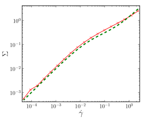
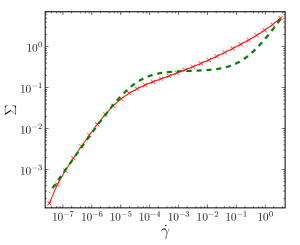
Refer to caption
(a) ϕeff=0.519subscriptitalic-ϕeff0.519\phi_{\mathrm{eff}}=0.519
Refer to caption
(b) ϕeff=0.600subscriptitalic-ϕeff0.600\phi_{\mathrm{eff}}=0.600
Refer to caption
(c) ϕeff=0.626subscriptitalic-ϕeff0.626\phi_{\mathrm{eff}}=0.626
Refer to caption
(d) ϕeff=0.639subscriptitalic-ϕeff0.639\phi_{\mathrm{eff}}=0.639
Refer to caption
(e) ϕeff=0.641subscriptitalic-ϕeff0.641\phi_{\mathrm{eff}}=0.641
Figure 2: Flow curves for different effective volume fractions. (Red lines with crosses) experimental measurements from Ref. [25]; (dashed green lines) fits with the WM-type model (see text); parameters are listed in Table I.
Stresses are given in units of Rh3kBTsuperscriptsubscript𝑅3subscript𝑘𝐵𝑇\frac{R_{h}^{3}}{k_{B}T}, where Rhsubscript𝑅R_{h} is the hydrodynamic radius of the colloids, and shear rates are non-dimensionalised with 6πηsolvRh3kBT6𝜋subscript𝜂solvsuperscriptsubscript𝑅3subscript𝑘𝐵𝑇\frac{6\pi\eta_{\mathrm{solv}}R_{h}^{3}}{k_{B}T}, with ηsolvsubscript𝜂solv\eta_{\mathrm{solv}} the solvent viscosity.
Refer to caption
(a) ϕeff=0.519subscriptitalic-ϕeff0.519\phi_{\mathrm{eff}}=0.519
Refer to caption
(b) ϕeff=0.600subscriptitalic-ϕeff0.600\phi_{\mathrm{eff}}=0.600
Refer to caption
(c) ϕeff=0.626subscriptitalic-ϕeff0.626\phi_{\mathrm{eff}}=0.626
Refer to caption
(d) ϕeff=0.639subscriptitalic-ϕeff0.639\phi_{\mathrm{eff}}=0.639
Refer to caption
(e) ϕeff=0.641subscriptitalic-ϕeff0.641\phi_{\mathrm{eff}}=0.641
Figure 3: Linear rheology measurements for different effective volume fractions. (Blue squares) experimental storage moduli G(ω)superscript𝐺𝜔G^{\prime}(\omega) from Ref. [25]; (dashed blue line) fit with the WM-type model (see text). (Green dots) experimental loss moduli G′′(ω)superscript𝐺′′𝜔G^{\prime\prime}(\omega); (dashed green line) fit with the WM-type model. The fitting parameters, as well as the stress and frequency units, are identical to those used in Fig. 2.
ϕeffsubscriptitalic-ϕeff\phi_{\mathrm{eff}} ταsubscript𝜏𝛼\tau_{\alpha} α𝛼\alpha η0subscript𝜂0\eta_{0} ηssubscript𝜂𝑠\eta_{s}
0.519 1.71.71.7 222222 9.09.09.0 1.21.21.2
0.600 900900900 353535 8.11038.1superscript1038.1\cdot 10^{3} 1.31.31.3
0.626 6.01046.0superscript1046.0\cdot 10^{4} 303030 5.41055.4superscript1055.4\cdot 10^{5} 1.51.51.5
0.639 8.01058.0superscript1058.0\cdot 10^{5} 303030 6.41066.4superscript1066.4\cdot 10^{6} 1.91.91.9
0.641 3.01063.0superscript1063.0\cdot 10^{6} 404040 4.81074.8superscript1074.8\cdot 10^{7} 2.02.02.0
Table 1: Model parameters used to fit the experimental flow curves in Fig. 2 and linear spectra in Fig. 3 .
As in Fig. 2, stresses are in units of Rh3kBTsuperscriptsubscript𝑅3subscript𝑘𝐵𝑇\frac{R_{h}^{3}}{k_{B}T} and times in units of kBT6πηsolvRh3subscript𝑘𝐵𝑇6𝜋subscript𝜂solvsuperscriptsubscript𝑅3\frac{k_{B}T}{6\pi\eta_{\mathrm{solv}}R_{h}^{3}}.

4.6 Base flow in Taylor-Couette geometry

Now, we focus on the base flow in a curved geometry, and more specifically in the Taylor-Couette cell used by Siebenbürger and colleagues in Ref. [25]. In such a rheometer, the fluid flows in the annular region between two co-axial cylinders, of radii ri=13.33mmsubscript𝑟𝑖13.33mmr_{i}=13.33\,\mathrm{mm} and ro=14.46mmsubscript𝑟𝑜14.46mmr_{o}=14.46\,\mathrm{mm} (relative gap width ϵ=0.085italic-ϵ0.085\epsilon=0.085), due to the rotation of the inner one. This geometry will be kept fixed for the rest of the paper.

Turning to the determination of the flow, we note that, unlike in Section 2, the velocity profile 𝒗(𝒓)𝒗𝒓\boldsymbol{v}(\boldsymbol{r}) is no longer prescribed. Therefore, we need to close the equations by complementing the WM-type constitutive equation, (Eq. 41) with the inertialess momentum conservation equation,

0=𝚺p,0𝚺𝑝0=\nabla\cdot\boldsymbol{\Sigma}-\nabla p, (44)

where p𝑝p is the pressure, and with the postulate of incompressibility,

0=𝒗.0𝒗0=\nabla\cdot\boldsymbol{v}. (45)

In the considered geometry, the base flow is purely azimuthal and has no dependence on θ𝜃\theta or z𝑧z, in cylindrical coordinates. It follows from Eq. 44 that the total shear stress must satisfy

Σ(r)=Σ(ri)ri2r2.Σ𝑟Σsubscript𝑟𝑖superscriptsubscript𝑟𝑖2superscript𝑟2\Sigma\left(r\right)=\Sigma\left(r_{i}\right)\frac{r_{i}^{2}}{r^{2}}.

Inversion of Eqs. 42 and 43 yields, for γ˙(ri)>0˙𝛾subscript𝑟𝑖0\dot{\gamma}(r_{i})>0,

γ˙(r)=12αηs[αταΣ(r)η0ηs+(η0+ηsαταΣ(r))2+4ηsαταΣ(r)],superscript˙𝛾𝑟12𝛼subscript𝜂𝑠delimited-[]𝛼subscript𝜏𝛼Σ𝑟subscript𝜂0subscript𝜂𝑠superscriptsubscript𝜂0subscript𝜂𝑠𝛼subscript𝜏𝛼Σ𝑟24subscript𝜂𝑠𝛼subscript𝜏𝛼Σ𝑟\dot{\gamma}^{\star}(r)=\frac{1}{2\alpha\eta_{s}}\left[\alpha\tau_{\alpha}\Sigma\left(r\right)-\eta_{0}-\eta_{s}+\sqrt{\left(\eta_{0}+\eta_{s}-\alpha\tau_{\alpha}\Sigma\left(r\right)\right)^{2}+4\eta_{s}\alpha\tau_{\alpha}\Sigma\left(r\right)}\right],

a profile of which is plotted in Fig. 4 for a particular applied shear rate. Since γ˙(r)vθvθrsuperscript˙𝛾𝑟superscriptsubscript𝑣𝜃superscriptsubscript𝑣𝜃𝑟\dot{\gamma}^{\star}(r)\equiv v_{\theta}^{\star\,\prime}-\frac{v_{\theta}^{\star}}{r}, we can solve numerically for the velocity profile vθ(r)subscript𝑣𝜃𝑟v_{\theta}(r). It is perhaps worth indicating that an analytical solution exists for ηs=0subscript𝜂𝑠0\eta_{s}=0:

vθ(r)=rαταlnυσα1Σ(r)υσα1Σ(r).superscriptsubscript𝑣𝜃𝑟𝑟𝛼subscript𝜏𝛼subscript𝜐𝜎superscript𝛼1Σ𝑟subscript𝜐𝜎superscript𝛼1Σ𝑟v_{\theta}^{\star}(r)=\frac{r}{\alpha\tau_{\alpha}}\ln\sqrt{\frac{\upsilon_{\sigma}\alpha^{-1}-\Sigma(r)}{\upsilon_{\sigma}\alpha^{-1}-\Sigma(r)}}. (46)

Incidentally, note that the quality of the approximation ηs=0subscript𝜂𝑠0\eta_{s}=0 is not fixed by the inequality ηsη0much-less-thansubscript𝜂𝑠subscript𝜂0\eta_{s}\ll\eta_{0}, but by the more stringent condition ηsη01+ατα|γ˙|much-less-thansubscript𝜂𝑠subscript𝜂01𝛼subscript𝜏𝛼superscript˙𝛾\eta_{s}\ll\frac{\eta_{0}}{1+\alpha\tau_{\alpha}|\dot{\gamma}^{\star}|}.

Refer to caption
Figure 4: Shear rate profile of the base flow in the Taylor-Couette cell, with model parameters corresponding to ϕeff=0.626subscriptitalic-ϕeff0.626\phi_{\mathrm{eff}}=0.626, for imposed (non-dimensional) shear rates at the rotor (blue) γ˙(ri)=105˙𝛾subscript𝑟𝑖superscript105\dot{\gamma}(r_{i})=10^{-5} and (green) γ˙(ri)=3104˙𝛾subscript𝑟𝑖3superscript104\dot{\gamma}(r_{i})=3\cdot 10^{-4}.

5 Shear-Thinning suppresses the visco-elastic instability

5.1 The visco-elastic instability

For almost one century, it has been known that the inertial flow of Newtonian liquids is prone to a centrifugal instability at large Reynolds numbers (or, more precisely, at large Taylor numbers), whereby counter-rotating vortices, known as “Taylor vortices”, appear and break the full cylindrical symmetry of the base flow [26, 27]. Shear-thinning fluids are also prone to this instability [28], which may even be enhanced, owing to shear-thinning, for polymeric solutions [29].

This type of instability is driven by inertia and opposed by viscosity. In dense colloidal suspensions, the vanishing Reynolds number precludes it. Yet, there exists a distinct type of instability, which does not require inertia: the so called visco-elastic instability was first analysed by Muller, Larson and Shaqfeh [3, 30, 31] and has notably been observed in polymer solutions [3] and (semi-dilute) worm-like micellar solutions [4], in Taylor-Couette, cone-and-plate and parallel-plate rheometers (for a review, see Ref. [32]). To grasp the importance of this finding, one should remember that, for decades, scientists have measured the rheological properties of polymer solutions and polymer melts in such setups, under the assumption of a well-defined (base) flow.

The precise mechanism driving the instability is still, to some extent, unsettled, but it is clear that curved streamlines and material elasticity (i.e., a finite structural relaxation time) are vital for the (linear) instability to develop. Indeed, because of the curvature in, say, a cylindrical setup, the normal stress ΣθθsubscriptΣ𝜃𝜃\Sigma_{\theta\theta} is coupled to the radial velocity component; this can lead to a positive feedback mechanism, whereby a spontaneous radial velocity perturbation alters ΣθθsubscriptΣ𝜃𝜃\Sigma_{\theta\theta}, which further amplifies the perturbation [32]. To assess the effect of the material’s properties on the instability, Larson used a model featuring a distribution of relaxation times and an adjustable shear-thinning exponent, and showed that shear-thinning tends to stabilise the flow, by shifting the unstable region (in parameter space) to larger applied shear rates [33]. Nevertheless, the author noted that “an elastic instability can occur even in highly shear-thinning entangled polymer solutions”, in the light of his calculations and experiments. Clearly, we are interested in knowing whether this also holds true for highly concentrated colloidal suspensions: Does the dramatic shear-thinning behaviour of these materials allow for a visco-elastic instability within the experimentally probed range of shear rates, according to the model introduced in the previous section?

5.2 Pseudo-spectral method for linear stability analysis

To address this question, we analyse the stability of the base flow in Taylor-Couette geometry (see Section 4.6) with respect to linear perturbations. Although many studies have focused only on axisymmetric instabilities, non-axisymmetric modes were shown to be even more unstable in a number of cases [34, 35], so we investigate three-dimensional perturbations, i.e., perturbations δϕ𝛿italic-ϕ\delta\phi with a spatial dependence not only on r𝑟r and z𝑧z, but also on θ𝜃\theta, viz.,

δϕ(r,θ,z,t)(δσrrδσrθδσrzδσθθδσθzδσzzδvrδvθδvzδp).𝛿italic-ϕ𝑟𝜃𝑧𝑡superscript𝛿subscript𝜎𝑟𝑟𝛿subscript𝜎𝑟𝜃𝛿subscript𝜎𝑟𝑧𝛿subscript𝜎𝜃𝜃𝛿subscript𝜎𝜃𝑧𝛿subscript𝜎𝑧𝑧𝛿subscript𝑣𝑟𝛿subscript𝑣𝜃𝛿subscript𝑣𝑧𝛿𝑝top\delta\phi(r,\theta,z,t)\equiv\left(\begin{array}[]{cccccccccc}\delta\sigma_{rr}&\delta\sigma_{r\theta}&\delta\sigma_{rz}&\delta\sigma_{\theta\theta}&\delta\sigma_{\theta z}&\delta\sigma_{zz}&\delta v_{r}&\delta v_{\theta}&\delta v_{z}&\delta p\end{array}\right)^{\top}.

We resort to a pseudo-spectral method.

(i) We start by linearising the equations of the problem, comprising the six constitutive equations (Eqs. 41), the three momentum conservation equations (Eqs. 44), and the incompressibility postulate (Eq. 45), around the base flow so as to obtain a system of linear equations of the form

(tt0000)𝒜δϕ=δϕ.𝒜𝑡missing-subexpressionmissing-subexpressionmissing-subexpressionmissing-subexpressionmissing-subexpressionmissing-subexpressionmissing-subexpressionmissing-subexpressionmissing-subexpressionmissing-subexpressionmissing-subexpressionmissing-subexpressionmissing-subexpressionmissing-subexpression𝑡missing-subexpressionmissing-subexpressionmissing-subexpressionmissing-subexpressionmissing-subexpressionmissing-subexpressionmissing-subexpression0missing-subexpressionmissing-subexpressionmissing-subexpressionmissing-subexpressionmissing-subexpressionmissing-subexpressionmissing-subexpression0missing-subexpressionmissing-subexpressionmissing-subexpressionmissing-subexpressionmissing-subexpressionmissing-subexpressionmissing-subexpression0missing-subexpressionmissing-subexpressionmissing-subexpressionmissing-subexpressionmissing-subexpressionmissing-subexpressionmissing-subexpression0𝛿italic-ϕsuperscript𝛿italic-ϕ\underset{\mathcal{A}}{\underbrace{\left(\begin{array}[]{ccccccc}\frac{\partial}{\partial t}\\ &\ddots\\ &&\frac{\partial}{\partial t}\\ &&&0\\ &&&&0\\ &&&&&0\\ &&&&&&0\end{array}\right)}}\delta\phi=\mathcal{L}^{\star}\delta\phi.

Then we transform the endomorphisms 𝒜𝒜\mathcal{A} and superscript\mathcal{L}^{\star} into matrices, viz., 𝒜𝐀𝒜𝐀\mathcal{A}\rightarrow{\bf A} and 𝐋superscriptsuperscript𝐋\mathcal{L}^{\star}\rightarrow{\bf L}^{\star}, with the following generic procedure:

(ii) δϕ𝛿italic-ϕ\delta\phi is Fourier-transformed both in the azimuthal direction (wavenumber m𝑚m) and in the axial direction (wavenumber k𝑘k), viz.,

δϕ(r,θ,z,t)=m=k2π/Lzδϕ(r,m,k,t)eimθeikz,𝛿italic-ϕ𝑟𝜃𝑧𝑡superscriptsubscript𝑚subscript𝑘2𝜋subscript𝐿𝑧𝛿italic-ϕ𝑟𝑚𝑘𝑡superscript𝑒𝑖𝑚𝜃superscript𝑒𝑖𝑘𝑧\delta\phi(r,\theta,z,t)=\sum_{m=-\infty}^{\infty}\sum_{k\in\nicefrac{{2\pi}}{{L_{z}}}\mathbb{Z}}\delta\phi(r,m,k,t)\,e^{im\theta}e^{ikz},

(iii) δϕ𝛿italic-ϕ\delta\phi is discretised along the radial coordinate r𝑟r by sampling its values at the Chebyshev–Gauss–Lobatto points rn1.0+ϵ2[1+cos(πnM)], 0n<Mformulae-sequencesubscript𝑟𝑛1.0italic-ϵ2delimited-[]1cos𝜋𝑛𝑀 0𝑛𝑀r_{n}\equiv 1.0+\frac{\epsilon}{2}\left[1+\mathrm{cos}\left(\pi\frac{n}{M}\right)\right],\,0\leqslant n<M, for a given M𝑀superscriptM\in\mathbb{N}^{\star}. We will typically use M26𝑀superscript26M\approx 2^{6} interpolation points across the gap. Radial derivatives rδϕsubscript𝑟𝛿italic-ϕ\partial_{r}\delta\phi are then written as matrix-vector products of the form Drδϕsubscript𝐷𝑟𝛿italic-ϕD_{r}\cdot\delta\phi [36].

(iv) δϕ𝛿italic-ϕ\delta\phi is Laplace-transformed with respect to time, with Laplace coordinate s𝑠s, viz., δϕ(r,m,k,s)=estδϕ(r,m,k,t)𝑑t𝛿italic-ϕ𝑟𝑚𝑘𝑠superscript𝑒𝑠𝑡𝛿italic-ϕ𝑟𝑚𝑘𝑡differential-d𝑡\delta\phi(r,m,k,s)=\int e^{st}\delta\phi(r,m,k,t)dt.

Eventually, one obtains the following generalised eigenvalue problem,

𝐀δϕ(r,m,k,s)=s𝐋δϕ(r,m,k,s),𝐀𝛿italic-ϕ𝑟𝑚𝑘𝑠𝑠superscript𝐋𝛿italic-ϕ𝑟𝑚𝑘𝑠{\bf A}\delta\phi(r,m,k,s)=s{\bf L}^{\star}\delta\phi(r,m,k,s), (47)

where 𝐀𝐀{\bf A} and 𝐋superscript𝐋{\bf L}^{\star} are 10M×10M10𝑀10𝑀10M\times 10M matrices, a few lines of which are subsequently substituted for the implementation of the (no-slip) boundary conditions on the velocity.

Let ssuperscript𝑠s^{\star} be the maximal growth rate, i.e., the real part of the maximal eigenvalue333 Due to the discretisation, some spurious eigenvalues may pop up in the generalised eigenvalue problem (Eq. 47), but they can easily be eliminated because, unlike their physical counterparts, they vary with the number of discretisation points. of Eq. 47 over all possible wavenumbers m𝑚m and k𝑘k. Then the base flow is (linearly) stable if, and only if, s<0superscript𝑠0s^{\star}<0.

5.3 Linearised equations

The linearised constitutive equations read:

δσrrt𝛿subscript𝜎𝑟𝑟𝑡\displaystyle\frac{\partial\delta\sigma_{rr}}{\partial t} =\displaystyle= (1τimrvθ)δσrr+(2σrθimr+2υσr)δvr1superscript𝜏𝑖𝑚𝑟superscriptsubscript𝑣𝜃𝛿subscript𝜎𝑟𝑟2superscriptsubscript𝜎𝑟𝜃𝑖𝑚𝑟2subscript𝜐𝜎subscript𝑟𝛿subscript𝑣𝑟\displaystyle\left(\frac{-1}{\tau^{\star}}-\frac{im}{r}v_{\theta}^{\star}\right)\delta\sigma_{rr}+\left(2\sigma_{r\theta}^{\star}\frac{im}{r}+2\upsilon_{\sigma}\partial_{r}\right)\delta v_{r}
δσrθt𝛿subscript𝜎𝑟𝜃𝑡\displaystyle\frac{\partial\delta\sigma_{r\theta}}{\partial t} =\displaystyle= γ˙δσrr+(1τimrvθ)δσrθ+[σrθimr+υσ(r1r)ασrθ(r1r)]δvθsuperscript˙𝛾𝛿subscript𝜎𝑟𝑟1superscript𝜏𝑖𝑚𝑟superscriptsubscript𝑣𝜃𝛿subscript𝜎𝑟𝜃delimited-[]superscriptsubscript𝜎𝑟𝜃𝑖𝑚𝑟subscript𝜐𝜎subscript𝑟1𝑟𝛼superscriptsubscript𝜎𝑟𝜃subscript𝑟1𝑟𝛿subscript𝑣𝜃\displaystyle\dot{\gamma}^{\star}\delta\sigma_{rr}+\left(\frac{-1}{\tau^{\star}}-\frac{im}{r}v_{\theta}^{\star}\right)\delta\sigma_{r\theta}+\left[\sigma_{r\theta}^{\star}\frac{im}{r}+\upsilon_{\sigma}\left(\partial_{r}-\frac{1}{r}\right)-\alpha\sigma_{r\theta}^{\star}\left(\partial_{r}-\frac{1}{r}\right)\right]\delta v_{\theta}
+[σrθ(r+1r)rσrθ+σθθimr+υσimrασrθimr]δvrdelimited-[]superscriptsubscript𝜎𝑟𝜃subscript𝑟1𝑟subscript𝑟superscriptsubscript𝜎𝑟𝜃superscriptsubscript𝜎𝜃𝜃𝑖𝑚𝑟subscript𝜐𝜎𝑖𝑚𝑟𝛼superscriptsubscript𝜎𝑟𝜃𝑖𝑚𝑟𝛿subscript𝑣𝑟\displaystyle+\left[\sigma_{r\theta}^{\star}\left(\partial_{r}+\frac{1}{r}\right)-\partial_{r}\sigma_{r\theta}^{\star}+\sigma_{\theta\theta}^{\star}\frac{im}{r}+\upsilon_{\sigma}\frac{im}{r}-\alpha\sigma_{r\theta}^{\star}\frac{im}{r}\right]\delta v_{r}
δσrzt𝛿subscript𝜎𝑟𝑧𝑡\displaystyle\frac{\partial\delta\sigma_{rz}}{\partial t} =\displaystyle= (1τimrvθ)δσrz+ikυσδvr+(σrθimr+υσr)δvz1superscript𝜏𝑖𝑚𝑟superscriptsubscript𝑣𝜃𝛿subscript𝜎𝑟𝑧𝑖𝑘subscript𝜐𝜎𝛿subscript𝑣𝑟superscriptsubscript𝜎𝑟𝜃𝑖𝑚𝑟subscript𝜐𝜎subscript𝑟𝛿subscript𝑣𝑧\displaystyle\left(\frac{-1}{\tau^{\star}}-\frac{im}{r}v_{\theta}^{\star}\right)\delta\sigma_{rz}+ik\upsilon_{\sigma}\delta v_{r}+\left(\sigma_{r\theta}^{\star}\frac{im}{r}+\upsilon_{\sigma}\partial_{r}\right)\delta v_{z}
δσθθt𝛿subscript𝜎𝜃𝜃𝑡\displaystyle\frac{\partial\delta\sigma_{\theta\theta}}{\partial t} =\displaystyle= 2γ˙δσrθ+(1τimrvθ)δσθθ+(2σθθrrσθθ+2υσrασθθimr)δvr2superscript˙𝛾𝛿subscript𝜎𝑟𝜃1superscript𝜏𝑖𝑚𝑟superscriptsubscript𝑣𝜃𝛿subscript𝜎𝜃𝜃2superscriptsubscript𝜎𝜃𝜃𝑟subscript𝑟superscriptsubscript𝜎𝜃𝜃2subscript𝜐𝜎𝑟𝛼superscriptsubscript𝜎𝜃𝜃𝑖𝑚𝑟𝛿subscript𝑣𝑟\displaystyle 2\dot{\gamma}^{\star}\delta\sigma_{r\theta}+\left(\frac{-1}{\tau^{\star}}-\frac{im}{r}v_{\theta}^{\star}\right)\delta\sigma_{\theta\theta}+\left(\frac{2\sigma_{\theta\theta}^{\star}}{r}-\partial_{r}\sigma_{\theta\theta}^{\star}+\frac{2\upsilon_{\sigma}}{r}-\alpha\sigma_{\theta\theta}^{\star}\frac{im}{r}\right)\delta v_{r}
+[2σrθ(r1/r)+2σθθimr+2υσimrασθθ(r1r)]δvθdelimited-[]2superscriptsubscript𝜎𝑟𝜃subscript𝑟1𝑟2superscriptsubscript𝜎𝜃𝜃𝑖𝑚𝑟2subscript𝜐𝜎𝑖𝑚𝑟𝛼superscriptsubscript𝜎𝜃𝜃subscript𝑟1𝑟𝛿subscript𝑣𝜃\displaystyle+\left[2\sigma_{r\theta}^{\star}(\partial_{r}-\nicefrac{{1}}{{r}})+2\sigma_{\theta\theta}^{\star}\frac{im}{r}+2\upsilon_{\sigma}\frac{im}{r}-\alpha\sigma_{\theta\theta}^{\star}\left(\partial_{r}-\frac{1}{r}\right)\right]\delta v_{\theta}
δσθzt𝛿subscript𝜎𝜃𝑧𝑡\displaystyle\frac{\partial\delta\sigma_{\theta z}}{\partial t} =\displaystyle= γ˙δσrz+(1τimrvθ)δσθz+ikυσδvθ+(υσimr+σθθimr+σrθr)δvzsuperscript˙𝛾𝛿subscript𝜎𝑟𝑧1superscript𝜏𝑖𝑚𝑟superscriptsubscript𝑣𝜃𝛿subscript𝜎𝜃𝑧𝑖𝑘subscript𝜐𝜎𝛿subscript𝑣𝜃subscript𝜐𝜎𝑖𝑚𝑟superscriptsubscript𝜎𝜃𝜃𝑖𝑚𝑟superscriptsubscript𝜎𝑟𝜃subscript𝑟𝛿subscript𝑣𝑧\displaystyle\dot{\gamma}^{\star}\delta\sigma_{rz}+\left(\frac{-1}{\tau^{\star}}-\frac{im}{r}v_{\theta}^{\star}\right)\delta\sigma_{\theta z}+ik\upsilon_{\sigma}\delta v_{\theta}+\left(\upsilon_{\sigma}\frac{im}{r}+\sigma_{\theta\theta}^{\star}\frac{im}{r}+\sigma_{r\theta}^{\star}\partial_{r}\right)\delta v_{z}
δσzzt𝛿subscript𝜎𝑧𝑧𝑡\displaystyle\frac{\partial\delta\sigma_{zz}}{\partial t} =\displaystyle= (1τimrvθ)δσzz+2ikυσδvz,1superscript𝜏𝑖𝑚𝑟superscriptsubscript𝑣𝜃𝛿subscript𝜎𝑧𝑧2𝑖𝑘subscript𝜐𝜎𝛿subscript𝑣𝑧\displaystyle\left(\frac{-1}{\tau^{\star}}-\frac{im}{r}v_{\theta}^{\star}\right)\delta\sigma_{zz}+2ik\upsilon_{\sigma}\delta v_{z},

where ττα1+αταγ˙superscript𝜏subscript𝜏𝛼1𝛼subscript𝜏𝛼superscript˙𝛾\tau^{\star}\equiv\frac{\tau_{\alpha}}{1+\alpha\tau_{\alpha}\dot{\gamma}^{\star}}, while the linearised momentum conservation equations are

00\displaystyle 0 =\displaystyle= (r+1r)δσrr+imrδσrθ+ikδσrz1rδσθθrδpsubscript𝑟1𝑟𝛿subscript𝜎𝑟𝑟𝑖𝑚𝑟𝛿subscript𝜎𝑟𝜃𝑖𝑘𝛿subscript𝜎𝑟𝑧1𝑟𝛿subscript𝜎𝜃𝜃subscript𝑟𝛿𝑝\displaystyle\left(\partial_{r}+\frac{1}{r}\right)\delta\sigma_{rr}+\frac{im}{r}\delta\sigma_{r\theta}+ik\delta\sigma_{rz}-\frac{1}{r}\delta\sigma_{\theta\theta}-\partial_{r}\delta p
+ηs[r2+1rr1r2m2r2k2]δvr2ηsimr2δvθsubscript𝜂𝑠delimited-[]superscriptsubscript𝑟21𝑟subscript𝑟1superscript𝑟2superscript𝑚2superscript𝑟2superscript𝑘2𝛿subscript𝑣𝑟2subscript𝜂𝑠𝑖𝑚superscript𝑟2𝛿subscript𝑣𝜃\displaystyle+\eta_{s}\left[\partial_{r}^{2}+\frac{1}{r}\partial_{r}-\frac{1}{r^{2}}-\frac{m^{2}}{r^{2}}-k^{2}\right]\delta v_{r}-2\eta_{s}\frac{im}{r^{2}}\delta v_{\theta}
00\displaystyle 0 =\displaystyle= (r+2r)δσrθ+imrδσθθ+ikδσθzimrδpsubscript𝑟2𝑟𝛿subscript𝜎𝑟𝜃𝑖𝑚𝑟𝛿subscript𝜎𝜃𝜃𝑖𝑘𝛿subscript𝜎𝜃𝑧𝑖𝑚𝑟𝛿𝑝\displaystyle\left(\partial_{r}+\frac{2}{r}\right)\delta\sigma_{r\theta}+\frac{im}{r}\delta\sigma_{\theta\theta}+ik\delta\sigma_{\theta z}-\frac{im}{r}\delta p
+ηs[r2+1rrm2r21r2k2]δvθ+2ηsimr2δvrsubscript𝜂𝑠delimited-[]superscriptsubscript𝑟21𝑟subscript𝑟superscript𝑚2superscript𝑟21superscript𝑟2superscript𝑘2𝛿subscript𝑣𝜃2subscript𝜂𝑠𝑖𝑚superscript𝑟2𝛿subscript𝑣𝑟\displaystyle+\eta_{s}\left[\partial_{r}^{2}+\frac{1}{r}\partial_{r}-\frac{m^{2}}{r^{2}}-\frac{1}{r^{2}}-k^{2}\right]\delta v_{\theta}+2\eta_{s}\frac{im}{r^{2}}\delta v_{r}
00\displaystyle 0 =\displaystyle= (r+1r)δσrz+imrδσθz+ikδσzzikδp,subscript𝑟1𝑟𝛿subscript𝜎𝑟𝑧𝑖𝑚𝑟𝛿subscript𝜎𝜃𝑧𝑖𝑘𝛿subscript𝜎𝑧𝑧𝑖𝑘𝛿𝑝\displaystyle\left(\partial_{r}+\frac{1}{r}\right)\delta\sigma_{rz}+\frac{im}{r}\delta\sigma_{\theta z}+ik\delta\sigma_{zz}-ik\delta p,
+ηs[r2+1rrm2r2k2]δvzsubscript𝜂𝑠delimited-[]superscriptsubscript𝑟21𝑟subscript𝑟superscript𝑚2superscript𝑟2superscript𝑘2𝛿subscript𝑣𝑧\displaystyle+\eta_{s}\left[\partial_{r}^{2}+\frac{1}{r}\partial_{r}-\frac{m^{2}}{r^{2}}-k^{2}\right]\delta v_{z}

and incompressibility states that

0=(r+1r)δvr+imrδvθ+ikδvz.0subscript𝑟1𝑟𝛿subscript𝑣𝑟𝑖𝑚𝑟𝛿subscript𝑣𝜃𝑖𝑘𝛿subscript𝑣𝑧0=\left(\partial_{r}+\frac{1}{r}\right)\delta v_{r}+\frac{im}{r}\delta v_{\theta}+ik\delta v_{z}.

When the shear-thinning parameter α𝛼\alpha vanishes, these linear equations reduce to those derived by Avgousti and Beris [34] for an Oldroyd-B fluid; as a matter of fact, we have spotted slight differences with Ref. [34], which we believe are typos in that publication.

These equations involve three non-dimensional quantities: the shear-thinning parameter α𝛼\alpha, the “bare Weissenberg” number ταγ˙subscript𝜏𝛼superscript˙𝛾\tau_{\alpha}\dot{\gamma}^{\star}, and the relative Newtonian viscosity ηs/η0subscript𝜂𝑠subscript𝜂0\nicefrac{{\eta_{s}}}{{\eta_{0}}}, on top of the (fixed) relative curvature ϵitalic-ϵ\epsilon.

5.4 Linear stability analysis: general trends and application to dense suspensions

5.4.1 Consistency of the algorithm for α0𝛼0\alpha\rightarrow 0, ηs0subscript𝜂𝑠0\eta_{s}\rightarrow 0 and influence of the shear rate

To check the validity of our algorithm, we have first set the shear-thinning parameter α𝛼\alpha and the Newtonian viscosity ηssubscript𝜂𝑠\eta_{s} to values close to zero. A conventional Upper Convected Maxwell (UCM) model should then be recovered, in which case, following Ref. [30], some axisymmetric modes (at m=0𝑚0m=0) become unstable at sufficiently large applied shear rates. This is indeed the case in our simulations, as soon as the shear rate grows larger than a critical shear rate comparable to that reported in Ref. [30]. However, we also observe that some non-axisymmetric modes, associated to small azimuthal wavenumbers m=𝒪(1)𝑚𝒪1m=\mathcal{O}(1), are even more unstable than the axisymmetric ones, in accordance with the literature [34]. Figure 5 shows the increase of the growth rate ssuperscript𝑠s^{\text{$\star$}} of the most unstable mode with the shear rate γ˙˙𝛾\dot{\gamma} measured at the inner cylinder (or the “bare Weissenberg” number ταγ˙subscript𝜏𝛼˙𝛾\tau_{\alpha}\dot{\gamma}).

Refer to caption
(a) ssuperscript𝑠s^{\star} vs. applied shear rate γ˙˙𝛾\dot{\gamma} for vanishing Newtonian viscosity (ηs/η0=106subscript𝜂𝑠subscript𝜂0superscript106\nicefrac{{\eta_{s}}}{{\eta_{0}}}=10^{-6}) (UCM model).
Refer to caption
(b) ssuperscript𝑠s^{\star} vs. ηssubscript𝜂𝑠\eta_{s}, at fixed shear rate (γ˙=20˙𝛾20\dot{\gamma}=20).
Figure 5: Maximal growth rate ssuperscript𝑠s^{\star} (over all modes) in the limit of a non-shear-thinning fluid, α=3104𝛼3superscript104\alpha=3\cdot 10^{-4}, τα=1.4subscript𝜏𝛼1.4\tau_{\alpha}=1.4. At γ˙=20˙𝛾20\dot{\gamma}=20, the most unstable modes are at m1similar-to-or-equals𝑚1m\simeq 1, k70similar-to-or-equals𝑘70k\simeq 70. The dashed red line separates stable base flows (below the line) from unstable ones (above).

5.4.2 Stabilising effect of the Newtonian viscosity

Including a Newtonian contribution to the stress, via a finite value of the viscosity ηssubscript𝜂𝑠\eta_{s}, tends to stabilise the flow, as shown in Fig. 5b. This stabilising role has already been reported in the literature on the Oldroyd-B model (i.e., for α=0𝛼0\alpha=0) [34, 32]; we find that it holds true for shear-thinning fluids, i.e., when α𝛼\alpha departs from zero (see Fig. 6).

Refer to caption
Figure 6: Dependence of the maximal growth rate ssuperscript𝑠s^{\star} on the Newtonian viscosity ηssubscript𝜂𝑠\eta_{s}, for a shear-thinning fluid with the following parameters: α=7.7𝛼7.7\alpha=7.7, τα=1.4subscript𝜏𝛼1.4\tau_{\alpha}=1.4, γ˙=20˙𝛾20\dot{\gamma}=20. (The growth rates vary only weakly with k𝑘k and m𝑚m for these parameters; only modes m250𝑚250m\leqslant 250 are considered here).

5.4.3 Stabilisation through shear-thinning

For the values of α𝛼\alpha of interest here, shear-thinning strongly suppresses the instability. Figures 7-8 show that, for the model parameters corresponding to the colloidal suspension at ϕeff=0.519subscriptitalic-ϕeff0.519\phi_{\mathrm{eff}}=0.519, but with vanishing Newtonian viscosity, the base flow lies deep within the stable region, whereas, in the absence of shear-thinning, i.e., were α𝛼\alpha vanishingly small, a linear instability would develop, with a peak of instability around k70similar-to-or-equals𝑘70k\simeq 70, m1similar-to-or-equals𝑚1m\simeq 1.

We should however mention the existence of a limited range of values of α𝛼\alpha, outside the experimentally relevant window for dense colloidal suspensions, namely, 0.3α3less-than-or-similar-to0.3𝛼less-than-or-similar-to30.3\lesssim\alpha\lesssim 3 and marked by red vertical bars on Fig. 7, which display unstable modes associated to abnormally large growth rates. These modes are located in a very different region of the (k,m)𝑘𝑚(k,m)-plane, namely k0𝑘0k\approx 0 and m1much-greater-than𝑚1m\gg 1. Although these perturbations have reasonable shapes in space, it is plausible that they are actually unphysical, but we do not know whether they are intrinsic in our WM-model or whether they arise because of artifacts in the (well established) numerical method. In the following, we concentrate on the experimentally relevant range of parameters.
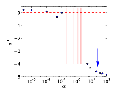
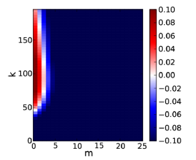
Refer to caption
Figure 7: Dependence of the maximal growth rate ssuperscript𝑠s^{\star} on the shear-thinning parameter α𝛼\alpha, for ηs/η0=106subscript𝜂𝑠subscript𝜂0superscript106\nicefrac{{\eta_{s}}}{{\eta_{0}}}=10^{-6}, τα=1.4subscript𝜏𝛼1.4\tau_{\alpha}=1.4, γ˙=20˙𝛾20\dot{\gamma}=20. The arrow points to the typical values of α𝛼\alpha of interest here. See the text for the description of the red vertical bars.
Refer to caption
(a) α=3104𝛼3superscript104\alpha=3\cdot 10^{-4}
Refer to caption
(b) α=102𝛼superscript102\alpha=10^{-2}
Figure 8: Colour maps of the maximal growth rates associated with each pair of wavenumbers (m,k)𝑚𝑘(m,k) for two distinct, but small, values of α𝛼\alpha (see captions), at γ˙=20˙𝛾20\dot{\gamma}=20, with negligible Newtonian viscosity (ηs/η0=106subscript𝜂𝑠subscript𝜂0superscript106\nicefrac{{\eta_{s}}}{{\eta_{0}}}=10^{-6}). Stable modes appear in dark blue.

5.4.4 Linear stability analysis of dense colloidal suspensions

We now specifically consider the model parameters used to fit the rheology of dense colloidal suspensions, (see Table 1).

Consistently with the strongly stabilising effect of shear-thinning described in the previous section (Section 5.4.3), we have numerically ascertained the stability of the base flows corresponding to the suspension at ϕ=0.519italic-ϕ0.519\phi=0.519 for rescaled shear rates γ˙=104, 102, 101˙𝛾superscript104superscript102superscript101\dot{\gamma}=10^{-4},\,10^{-2},\,10^{-1}, at ϕeff=0.626subscriptitalic-ϕeff0.626\phi_{\mathrm{eff}}=0.626 for γ˙=5106, 5104, 5103, 102˙𝛾5superscript1065superscript1045superscript103superscript102\dot{\gamma}=5\cdot 10^{-6},\,5\cdot 10^{-4},\,5\cdot 10^{-3},\,10^{-2} in the experimental range, as well as that with effective volume fraction ϕeff=0.641subscriptitalic-ϕeff0.641\phi_{\mathrm{eff}}=0.641 at γ˙=108, 106, 104˙𝛾superscript108superscript106superscript104\dot{\gamma}=10^{-8},\,10^{-6},\,10^{-4}. The relative contribution of the Newtonian viscosity to the stabilisation of the flow echoes the contribution of the Newtonian stress to the total stress: at high densities and low shear rates, the effect of the Newtonian viscosity is negligible. Admittedly, the more acute shear-thinning displayed by the WM models fitted to the densest suspensions results in an enhanced stability compared to the experimental systems; however the fact that they lie so deep in the stable region suggests that the materials they model, albeit somewhat less shear-thinning, are also stable with respect to the considered perturbations. This is further supported by the observed stability of the system at ϕ=0.519italic-ϕ0.519\phi=0.519, which is both less shear-thinning than the others and very well described by the WM model.

5.5 Rationalisation with the Pakdel-McKinley criterion

Before we conclude, it is interesting to note that the stabilising effects of shear-thinning and of the Newtonian contribution are in line with the visco-elastic stability criterion proposed by Pakdel and McKinley in 1996 [37, 38] (less general versions of the criterion can be found in earlier publications [30]). On the basis of a dimensional analysis of generic visco-elastic constitutive equations, these authors introduced a dimensionless number, written 𝒫𝒫\mathcal{P} here, for inertialess visco-elastic instabilities in curved geometries in analogy to the classical Taylor number for inertial instabilities, and propounded the idea that the base flow is susceptible to an instability if this dimensional number exceeds a given threshold of order unity. The Pakdel-McKinley number reads

𝒫lpN1Σ,𝒫subscript𝑙𝑝subscript𝑁1Σ\mathcal{P}\equiv\frac{l_{p}}{\mathcal{R}}\frac{N_{1}}{\Sigma},

where lpvθτsubscript𝑙𝑝subscript𝑣𝜃𝜏l_{p}\equiv v_{\theta}\tau is the typical distance travelled by a material substructure (e.g., a polymer chain) along the base-flow streamline while relaxing, \mathcal{R} is the radius of curvature of the streamline, N1subscript𝑁1N_{1} is the first normal-stress-difference and ΣΣ\Sigma is the shear stress. For a UCM model, the ratio N1Σsubscript𝑁1Σ\frac{N_{1}}{\Sigma} is simply the Weissenberg number and measures the “anisotropy of the normal forces”, as phrased by Morozov and van Saarloos [38]. But even with the present WM model, which is somewhat more complicated, the criterion based on 𝒫𝒫\mathcal{P} seems to capture the observed trends: a Newtonian contribution to the stress increases ΣΣ\Sigma without altering N1subscript𝑁1N_{1}, thereby reducing 𝒫𝒫\mathcal{P} and stabilising the flow. On the other hand, an enhanced propensity to shear-thinning results in a decrease of N1subscript𝑁1N_{1} as (1+αταγ˙)2superscript1𝛼subscript𝜏𝛼˙𝛾2\left(1+\alpha\tau_{\alpha}\dot{\gamma}\right)^{-2}, while ΣΣ\Sigma only decreases as (1+αταγ˙)1superscript1𝛼subscript𝜏𝛼˙𝛾1\left(1+\alpha\tau_{\alpha}\dot{\gamma}\right)^{-1} (for ηs0subscript𝜂𝑠0\eta_{s}\rightarrow 0); as a result, 𝒫𝒫\mathcal{P} is reduced, which also explains the enhanced stability of the flow.

The Newtonian stress contribution and the propensity to shear-thinning thus act in synergy, but, for the rheology of the very dense colloidal suspensions of interest here, our results indicate that the impact of shear-thinning quantitatively prevails over that of the former.


6 Discussion and Outlook

In conclusion, we have made use of, and partially extended, a general theoretical framework based on projections onto density modes, to describe the rheology of dense colloidal suspensions in the vicinity of the glass transition. Contrary to the previous theoretical works, which focused on strictly homogeneous flows, special attention was paid to the fate of spatial inhomogeneities. However, the intricacy of the formalism forced us to resort to particularly strong approximations before we could study the stability of the flow in curved (Taylor-Couette) geometry. At the expense of these approximations, constitutive equations falling in the White-Metzner class were obtained; the resulting model was shown to capture the shear-thinning properties of the material and to be reasonably consistent with experimental measurements of the linear rheology and steady-state rheology of the suspensions, although not in a strictly quantitative way. Eventually, we analysed the stability of the visco-elastic flow and brought evidence that, in the experimental range of shear rates, shear-thinning (and to a much lesser extent the Newtonian stress contribution) strongly stabilise the flow. This may explain why visco-elastic instabilities have been observed in a variety of visco-elastic fluids, but not in the dense suspensions under consideration here: the flow strains and destroys the microstructure of the material, so much so that, if a material volume is displaced by a perturbation, the memory of the stress that it carries, through its microstructure, is suppressed by the flow too quickly to allow the possibility of a feedback mechanism.


Acknowledgments

We thank Miriam Siebenbürger for providing us with the experimental rheological data. AN thanks Alexander Morozov for introducing him to the pseudo-spectral method, Fabian Frahsa for enlightening discussions, and the DFG-funded research unit FOR 1394 project P3 for partial funding of his stay at the University of Konstanz.

References

  • [1] P. Pusey and W. Van Megen, “Observation of a glass transition in suspensions of spherical colloidal particles,” Physical review letters, vol. 59, no. 18, p. 2083, 1987.
  • [2] C. Amann, M. Siebenbürger, M. Krüger, F. Weysser, M. Ballauff, and M. Fuchs, “Overshoots in stress-strain curves: Colloid experiments and schematic mode coupling theory,” Journal of Rheology, vol. 57, no. 1, p. 149, 2013.
  • [3] S. Muller, R. Larson, and E. Shaqfeh, “A purely elastic transition in taylor-couette flow,” Rheologica Acta, vol. 28, no. 6, pp. 499–503, 1989.
  • [4] M. Fardin, T. Ober, V. Grenard, T. Divoux, S. Manneville, G. McKinley, and S. Lerouge, “Interplay between elastic instabilities and shear-banding: three categories of Taylor-Couette flows and beyond,” Soft Matter, 2012.
  • [5] A. Einstein, “Eine neue bestimmung der moleküldimensionen,” Annalen der Physik, vol. 324, no. 2, pp. 289–306, 1906.
  • [6] G. Batchelor, “The effect of brownian motion on the bulk stress in a suspension of spherical particles,” Journal of Fluid Mechanics, vol. 83, no. 01, pp. 97–117, 1977.
  • [7] J. F. Brady, “Model hard-sphere dispersions: statistical mechanical theory, simulations, and experiments,” Current Opinion in Colloid & Interface Science, vol. 1, no. 4, pp. 472–480, 1996.
  • [8] J. M. Brader, “Nonlinear rheology of colloidal dispersions,” Journal of Physics: Condensed Matter, vol. 22, no. 36, p. 363101, 2010.
  • [9] U. Bengtzelius, W. Götze, and A. Sjolander, “Dynamics of supercooled liquids and the glass transition,” Journal of Physics C: Solid State Physics, vol. 17, no. 33, pp. 5915–5934, 1984.
  • [10] L. Sjögren, “Kinetic theory of current fluctuations in simple classical liquids,” Physical Review A, vol. 22, pp. 2866–2882, 1980.
  • [11] M. Fuchs and M. Cates, “Theory of Nonlinear Rheology and Yielding of Dense Colloidal Suspensions,” Physical Review Letters, vol. 89, no. 24, 2002.
  • [12] J. Brader, M. Cates, and M. Fuchs, “First-principles constitutive equation for suspension rheology,” Physical Review E, vol. 86, no. 2, p. 021403, 2012.
  • [13] K. Miyazaki, D. Reichman, and R. Yamamoto, “Supercooled liquids under shear: Theory and simulation,” Physical Review E, vol. 70, no. 1, p. 011501, 2004.
  • [14] C. Amann, M. Siebenbürger, M. Ballauff, and M. Fuchs, “Nonlinear rheology of glass-forming colloidal dispersions: transient stress–strain relations from anisotropic mode coupling theory and thermosensitive microgels,” Journal of Physics: Condensed Matter, vol. 27, no. 19, p. 194121, 2015.
  • [15] J. Brader, T. Voigtmann, M. Fuchs, R. Larson, and M. Cates, “Glass rheology: From mode-coupling theory to a dynamical yield criterion.,” Proceedings of the National Academy of Sciences of the United States of America, vol. 106, no. 36, pp. 15186–91, 2009.
  • [16] J. White and A. Metzner, “Development of constitutive equations for polymeric melts and solutions,” Journal of Applied Polymer Science, vol. 7, no. 5, pp. 1867–1889, 1963.
  • [17] M. Siebenbürger, M. Fuchs, and M. Ballauff, “Core–shell microgels as model colloids for rheological studies,” Soft Matter, vol. 8, no. 15, pp. 4014–4024, 2012.
  • [18] T. Voigtmann, “Nonlinear glassy rheology,” Current Opinion in Colloid & Interface Science, vol. 19, no. 6, pp. 549–560, 2014.
  • [19] H. Risken, The Fokker-Planck Equation. Methods of Solution and Applications. 1989.
  • [20] M. Fuchs and M. Cates, “A mode coupling theory for Brownian particles in homogeneous steady shear flow,” Journal of Rheology, vol. 53, no. 4, p. 957, 2009.
  • [21] J. Wu and J. Cao, “Gaussian factorization of hydrodynamic correlation functions and mode-coupling memory kernels,” Physical Review E, vol. 67, no. 6, p. 061116, 2003.
  • [22] R. Besseling, L. Isa, P. Ballesta, G. Petekidis, M. Cates, and W. Poon, “Shear banding and flow-concentration coupling in colloidal glasses,” Physical Review Letters, vol. 105, no. 26, p. 268301, 2010.
  • [23] H. Jin, K. Kang, K. H. Ahn, and J. K. Dhont, “Flow instability due to coupling of shear-gradients with concentration: non-uniform flow of (hard-sphere) glasses,” Soft Matter, vol. 10, no. 47, pp. 9470–9485, 2014.
  • [24] S. Papenkort and T. Voigtmann, “Channel flow of a tensorial shear-thinning maxwell model: Lattice boltzmann simulations,” The Journal of Chemical physics, vol. 140, no. 16, p. 164507, 2014.
  • [25] M. Siebenbürger, M. Fuchs, H. Winter, and M. Ballauff, “Viscoelasticity and shear flow of concentrated, noncrystallizing colloidal suspensions: Comparison with mode-coupling theory,” Journal of Rheology (1978-present), vol. 53, no. 3, pp. 707–726, 2009.
  • [26] G. Taylor, “Stability of a viscous liquid contained between two rotating cylinders,” Proceedings of the Royal Society of London. Series A, vol. 102, no. 718, pp. 541–542, 1923.
  • [27] M. A. Fardin, C. Perge, and N. Taberlet, “"the hydrogen atom of fluid dynamics" - introduction to the taylor-couette flow for soft matter scientists,” Soft Matter, vol. 10, pp. 3523–3535, 2014.
  • [28] O. Coronado-Matutti, P. S. Mendes, and M. Carvalho, “Instability of inelastic shear-thinning liquids in a couette flow between concentric cylinders,” Journal of fluids engineering, vol. 126, no. 3, pp. 385–390, 2004.
  • [29] R. Larson, “Taylor-couette stability analysis for a doi-edwards fluid,” Rheologica Acta, vol. 28, no. 6, pp. 504–510, 1989.
  • [30] R. Larson, E. Shaqfeh, and S. Muller, “A purely elastic instability in taylor–couette flow,” Journal of Fluid Mechanics, vol. 218, pp. 573–600, 1990.
  • [31] E. Shaqfeh, S. Muller, and R. Larson, “The effects of gap width and dilute solution properties on the viscoelastic Taylor-Couette instability,” Journal of Fluid Mechanics, vol. 235, no. -1, pp. 285–317, 1992.
  • [32] E. Shaqfeh, “Purely elastic instabilities in viscometric flows,” Annual Review of Fluid Mechanics, vol. 28, no. 1, pp. 129–185, 1996.
  • [33] R. Larson, “The effect of fluid rheology on the elastic Taylor-Couette instability,” Journal of Non-Newtonian Fluid Mechanics, vol. 51, no. 2, pp. 195–225, 1994.
  • [34] M. Avgousti, “Non-axisymmetric modes in viscoelastic taylor-couette flow,” Journal of Non-Newtonian Fluid Mechanics, vol. 50, no. 2-3, pp. 225–251, 1993.
  • [35] A. Nicolas and A. Morozov, “Nonaxisymmetric Instability of Shear-Banded Taylor-Couette Flow,” Physical Review Letters, vol. 108, no. 8, 2012.
  • [36] R. Peyret, Spectral methods for incompressible viscous flow, vol. 148. Springer Science & Business Media, 2002.
  • [37] P. Pakdel and G. McKinley, “Elastic instability and curved streamlines,” Physical Review Letters, vol. 77, no. 12, p. 2459, 1996.
  • [38] A. N. Morozov and W. van Saarloos, “An introductory essay on subcritical instabilities and the transition to turbulence in visco-elastic parallel shear flows,” Physics Reports, vol. 447, no. 3, pp. 112–143, 2007.

Appendix A Operator formulation of the switch to the auxiliary frame

In Section 2.2, the switch to the auxiliary frame at a specific point was presented as a change of coordinates. However, it may also be conducted with the operator formalism. Indeed, consider an auxiliary system (denoted by tildes) with the following Smoluchowski operator

Ω~(Γ,t)i=1N[i+𝑭𝒊(Γ)+𝒗~(𝒓𝒊,t)]i,superscript~ΩΓ𝑡superscriptsubscript𝑖1𝑁delimited-[]subscript𝑖subscript𝑭𝒊Γbold-~𝒗subscript𝒓𝒊𝑡subscript𝑖\tilde{\Omega}^{\dagger}(\Gamma,t)\equiv\sum_{i=1}^{N}\left[\partial_{i}+\boldsymbol{F_{i}}\left(\Gamma\right)+\boldsymbol{\tilde{v}}\left(\boldsymbol{r_{i}},t\right)\right]\cdot\partial_{i},

where

𝒗~(𝒓,t)𝒗solv(𝒓,t)𝒗solv(𝒓o(t),t).bold-~𝒗𝒓𝑡superscript𝒗solv𝒓𝑡superscript𝒗solvsubscript𝒓𝑜𝑡𝑡\boldsymbol{\tilde{v}}\left(\boldsymbol{r},t\right)\equiv\boldsymbol{v}^{\mathrm{solv}}\left(\boldsymbol{r},t\right)-\boldsymbol{v}^{\mathrm{solv}}\left(\boldsymbol{r}_{o}(t),t\right). (48)

As in Section 2.2, 𝒓o(t)subscript𝒓𝑜𝑡\boldsymbol{r}_{o}(t) is the position (given by Eq. 8) of the “material point” advected by the solvent flow field, with position 𝒓osubscript𝒓𝑜\boldsymbol{r}_{o} at tosubscript𝑡𝑜t_{o}.

In the auxiliary system, an observable g~(𝒓,Γ;t)~𝑔𝒓Γ𝑡\tilde{g}(\boldsymbol{r},\Gamma;t) evolves as

tg~(𝒓,Γ;t)subscript𝑡~𝑔𝒓Γ𝑡\displaystyle\partial_{t}\tilde{g}(\boldsymbol{r},\Gamma;t) =\displaystyle= Ω~(Γ,t)g~(𝒓,Γ;t).superscript~ΩΓ𝑡~𝑔𝒓Γ𝑡\displaystyle\tilde{\Omega}^{\dagger}(\Gamma,t)\tilde{g}(\boldsymbol{r},\Gamma;t).

Evaluating an observable in this auxiliary system is therefore equivalent to evaluating it in the auxiliary (denoted by primes) of Section 2.2: g~(𝒓,Γ;t)~𝑔𝒓Γ𝑡\tilde{g}(\boldsymbol{r},\Gamma;t) and g(𝒓,Γ;t)|Γ=Γevaluated-atsuperscript𝑔𝒓superscriptΓ𝑡superscriptΓΓg^{\prime}(\boldsymbol{r},\Gamma^{\prime};t)\Big{|}_{\Gamma^{\prime}=\Gamma} have the same time derivative Ω~(Γ,t)=Ω(Γ,t)|Γ=Γsuperscript~ΩΓ𝑡evaluated-atsuperscriptΩsuperscriptΓ𝑡superscriptΓΓ\tilde{\Omega}^{\dagger}(\Gamma,t)=\Omega^{\dagger\,\prime}(\Gamma^{\prime},t)\Big{|}_{\Gamma^{\prime}=\Gamma}, and they coincide at tosubscript𝑡𝑜t_{o}, so they are equal at all times.

The formal solution of Eq. 48 is

g~(𝒓,Γ;t)~𝑔𝒓Γ𝑡\displaystyle\tilde{g}(\boldsymbol{r},\Gamma;t) =\displaystyle= e0tΩ~(Γ,s)𝑑sg~(𝒓,Γ)superscriptsubscript𝑒superscriptsubscript0𝑡superscript~ΩΓ𝑠differential-d𝑠~𝑔𝒓Γ\displaystyle e_{-}^{\int_{0}^{t}\tilde{\Omega}^{\dagger}(\Gamma,s)ds}\tilde{g}(\boldsymbol{r},\Gamma)
=\displaystyle= e0tΩ~(Γ,s)𝑑sg(𝒓,Γ).superscriptsubscript𝑒superscriptsubscript0𝑡superscript~ΩΓ𝑠differential-d𝑠𝑔𝒓Γ\displaystyle e_{-}^{\int_{0}^{t}\tilde{\Omega}^{\dagger}(\Gamma,s)ds}g(\boldsymbol{r},\Gamma).

Using the shorthand A(t)superscript𝐴𝑡A^{\dagger}(t) for 𝒗solv(𝒓o(t),t)i=1Nisuperscript𝒗solvsubscript𝒓𝑜𝑡𝑡superscriptsubscript𝑖1𝑁subscript𝑖\boldsymbol{v}^{\mathrm{solv}}\left(\boldsymbol{r}_{o}(t),t\right)\cdot\sum_{i=1}^{N}\partial_{i}, we observe that A(t)superscript𝐴𝑡A^{\dagger}(t) commutes with all Ω(s)superscriptΩ𝑠\Omega^{\dagger}(s). Indeed,

Ω(s)A(t)gsuperscriptΩ𝑠superscript𝐴𝑡𝑔\displaystyle\Omega^{\dagger}(s)A^{\dagger}(t)g =\displaystyle= i=1N[i+𝑭𝒊(Γ)+𝒗solv(𝒓𝒊,s)]i[𝒗solv(𝒓o(t),t)j=1Njg]superscriptsubscript𝑖1𝑁delimited-[]subscript𝑖subscript𝑭𝒊Γsuperscript𝒗solvsubscript𝒓𝒊𝑠subscript𝑖delimited-[]superscript𝒗solvsubscript𝒓𝑜𝑡𝑡superscriptsubscript𝑗1𝑁subscript𝑗𝑔\displaystyle\sum_{i=1}^{N}\left[\partial_{i}+\boldsymbol{F_{i}}\left(\Gamma\right)+\boldsymbol{v}^{\mathrm{solv}}\left(\boldsymbol{r_{i}},s\right)\right]\cdot\partial_{i}\left[\boldsymbol{v}^{\mathrm{solv}}\left(\boldsymbol{r}_{o}(t),t\right)\cdot\sum_{j=1}^{N}\partial_{j}g\right]
=\displaystyle= 𝒗solv(𝒓o(t),t)i=1Nj=1N[jig+j(𝑭𝒊ig)+j𝒗solv(𝒓𝒊,s)ig],superscript𝒗solvsubscript𝒓𝑜𝑡𝑡superscriptsubscript𝑖1𝑁superscriptsubscript𝑗1𝑁delimited-[]subscript𝑗subscript𝑖𝑔subscript𝑗subscript𝑭𝒊subscript𝑖𝑔subscript𝑗superscript𝒗solvsubscript𝒓𝒊𝑠subscript𝑖𝑔\displaystyle\boldsymbol{v}^{\mathrm{solv}}\left(\boldsymbol{r}_{o}(t),t\right)\cdot\sum_{i=1}^{N}\sum_{j=1}^{N}\left[\partial_{j}\partial_{i}g+\partial_{j}\left(\boldsymbol{F_{i}}\cdot\partial_{i}g\right)+\partial_{j}\boldsymbol{v}^{\mathrm{solv}}\left(\boldsymbol{r_{i}},s\right)\partial_{i}g\right],
=\displaystyle= A(t)Ω(s)g,superscript𝐴𝑡superscriptΩ𝑠𝑔\displaystyle A^{\dagger}(t)\Omega^{\dagger}(s)g,

where we have made use of j𝒗solv(𝒓𝒋,s)=0subscript𝑗superscript𝒗solvsubscript𝒓𝒋𝑠0\partial_{j}\boldsymbol{v}^{\mathrm{solv}}\left(\boldsymbol{r_{j}},s\right)=0 and i=1N𝑭𝒊=0superscriptsubscript𝑖1𝑁subscript𝑭𝒊0\sum_{i=1}^{N}\boldsymbol{F_{i}}=0, hence j=1Ni=1Nj𝑭𝒊=𝟎superscriptsubscript𝑗1𝑁superscriptsubscript𝑖1𝑁subscript𝑗subscript𝑭𝒊0\sum_{j=1}^{N}\sum_{i=1}^{N}\partial_{j}\boldsymbol{F_{i}}=\boldsymbol{0}. It follows that

g~(𝒓,Γ;t)~𝑔𝒓Γ𝑡\displaystyle\tilde{g}(\boldsymbol{r},\Gamma;t) =\displaystyle= e0t𝑑s𝒗solv(𝒓o(s),s)i=1Nie0tΩ(Γ,s)𝑑sg(𝒓,Γ),superscriptsubscript𝑒superscriptsubscript0𝑡differential-d𝑠superscript𝒗solvsubscript𝒓𝑜𝑠𝑠superscriptsubscript𝑖1𝑁subscript𝑖superscriptsubscript𝑒superscriptsubscript0𝑡superscriptΩΓ𝑠differential-d𝑠𝑔𝒓Γ\displaystyle e_{-}^{-\int_{0}^{t}ds\boldsymbol{v}^{\mathrm{solv}}\left(\boldsymbol{r}_{o}(s),s\right)\cdot\sum_{i=1}^{N}\partial_{i}}e_{-}^{\int_{0}^{t}\Omega^{\dagger}(\Gamma,s)ds}g(\boldsymbol{r},\Gamma),
=\displaystyle= e0t𝑑s𝒗solv(𝒓o(s),s)i=1Nig(𝒓,Γ;t)superscriptsubscript𝑒superscriptsubscript0𝑡differential-d𝑠superscript𝒗solvsubscript𝒓𝑜𝑠𝑠superscriptsubscript𝑖1𝑁subscript𝑖𝑔𝒓Γ𝑡\displaystyle e_{-}^{-\int_{0}^{t}ds\boldsymbol{v}^{\mathrm{solv}}\left(\boldsymbol{r}_{o}(s),s\right)\cdot\sum_{i=1}^{N}\partial_{i}}g(\boldsymbol{r},\Gamma;t)

and, if g𝑔g does not depend intrinsically on space,

g~(𝒓,Γ;t)=e0t𝑑s𝒗solv(𝒓o(s),s)𝒓g(𝒓,Γ;t).~𝑔𝒓Γ𝑡superscriptsubscript𝑒superscriptsubscript0𝑡differential-d𝑠superscript𝒗solvsubscript𝒓𝑜𝑠𝑠subscript𝒓𝑔𝒓Γ𝑡\tilde{g}(\boldsymbol{r},\Gamma;t)=e_{-}^{\int_{0}^{t}ds\boldsymbol{v}^{\mathrm{solv}}\left(\boldsymbol{r}_{o}(s),s\right)\cdot\partial_{\boldsymbol{r}}}g(\boldsymbol{r},\Gamma;t).

In particular, the fluctuation advection term emerges when the equation is differentiated with respect to time.

tg(𝒓,Γ;t)=e0t𝑑s𝒗solv(𝒓o(s),s)𝒓tg~(𝒓,Γ;t)𝒗solv(𝒓o(t),t)𝒓g(𝒓,Γ;t).subscript𝑡𝑔𝒓Γ𝑡superscriptsubscript𝑒superscriptsubscript0𝑡differential-d𝑠superscript𝒗solvsubscript𝒓𝑜𝑠𝑠subscript𝒓subscript𝑡~𝑔𝒓Γ𝑡superscript𝒗solvsubscript𝒓𝑜𝑡𝑡subscript𝒓𝑔𝒓Γ𝑡\partial_{t}g(\boldsymbol{r},\Gamma;t)=e_{-}^{-\int_{0}^{t}ds\boldsymbol{v}^{\mathrm{solv}}\left(\boldsymbol{r}_{o}(s),s\right)\cdot\partial_{\boldsymbol{r}}}\partial_{t}\tilde{g}(\boldsymbol{r},\Gamma;t)-\boldsymbol{v}^{\mathrm{solv}}\left(\boldsymbol{r}_{o}(t),t\right)\cdot\partial_{\boldsymbol{r}}g(\boldsymbol{r},\Gamma;t).

This equation agrees with Eq. 14.