Optimized Projections for Compressed Sensing via Direct Mutual Coherence Minimization

Abstract

Compressed Sensing (CS) is a new data acquisition theory based on the existence of a sparse representation of a signal and a projected dictionary $\mathbf{P}\mathbf{D}$, where $\mathbf{P}\in\mathbb{R}^{m\times d}$ is the projection matrix and $\mathbf{D}\in\mathbb{R}^{d\times n}$ is the dictionary. To recover the signal from a small number $m$ of measurements, it is expected that the projected dictionary $\mathbf{P}\mathbf{D}$ is of low mutual coherence. Several previous methods attempt to find the projection $\mathbf{P}$ such that the mutual coherence of $\mathbf{P}\mathbf{D}$ is low. However, they do not minimize the mutual coherence directly and thus they may be far from optimal. Their used solvers lack convergence guarantee and thus the quality of their solutions is not guaranteed. This work aims to address these issues. We propose to find an optimal projection matrix by minimizing the mutual coherence of $\mathbf{P}\mathbf{D}$ directly. This leads to a nonconvex nonsmooth minimization problem. We approximate it by smoothing, solve it by alternating minimization and prove the convergence of our algorithm. To the best of our knowledge, this is the first work which directly minimizes the mutual coherence of the projected dictionary and has convergence guarantee. Numerical experiments demonstrate that our method can recover sparse signals better than existing ones.

1 Introduction

Compressed Sensing (CS) [1, 2] is a new sampling/data acquisition theory asserting that one can exploit sparsity or compressibility when acquiring signals of interest. It shows that signals which have a sparse representation with respect to appropriate bases can be recovered from a small number of measurements. A fundamental problem in CS is how to construct a measurement matrix such that the number of measurements is near minimal.

Consider a signal $\mathbf{x}\in\mathbb{R}^{d}$ which is assumed to have a sparse representation with respect to a fixed overcomplete dictionary $\mathbf{D}\in\mathbb{R}^{d\times n}$ $(d<n)$. This can be described as

$$\mathbf{x}=\mathbf{D}\bm{\alpha},$$ (1)

where $\bm{\alpha}\in\mathbb{R}^{n}$ is a sparse representation coefficient, i.e., $\left\lVert\bm{\alpha}\right\rVert_{0}\ll n$. Here $\left\lVert\bm{\alpha}\right\rVert_{0}$ denotes the $\ell_{0}$-norm which counts the number of nonzero elements in $\bm{\alpha}$. The solution to problem (1) is not unique since $d<n$. To find an appropriate solution in the solution set of (1), we need to use some additional structures of $\mathbf{D}$ and $\bm{\alpha}$. Considering that $\bm{\alpha}$ is sparse, we are interested in finding the sparsest representation coefficient $\bm{\alpha}$. This leads to the following sparse representation problem

$$\min_{\bm{\alpha}}\left\lVert\bm{\alpha}\right\rVert_{0},\ \operatorname*{s.t.}\ \mathbf{x}=\mathbf{D}\bm{\alpha}.$$ (2)

However, the above problem is NP-hard [3] and thus is challenging to solve. Some algorithms, such as Basis Pursuit (BP) [4] and Orthogonal Matching Pursuit (OMP) [5], can be used to find suboptimal solutions.

An interesting theoretical problem is that under what conditions the optimal solution to (2) can be computed. If the solution is computable, can it be exactly or approximately computed by BP or OMP? Some previous works answer the above questions based on the mutual coherence of the dictionary $\mathbf{D}$ [6].

Definition 1

Given $\mathbf{D}=[{\mathbf{d}}_{1},\cdots,\mathbf{d}_{n}]\in\mathbb{R}^{d\times n}$, its mutual coherence is defined as the largest absolute and normalized inner product between different columns of $\mathbf{D}$, i.e.,

$$\mu(\mathbf{D})=\max_{\begin{subarray}{c}1\leq i,j\leq n\\ i\neq j\end{subarray}}\frac{|\mathbf{d}_{i}^{T}\mathbf{d}_{j}|}{\left\lVert\mathbf{d}_{i}\right\rVert\left\lVert\mathbf{d}_{j}\right\rVert}.$$

The mutual coherence measures the highest correlation between any two columns of $\mathbf{D}$. It is expected to be as low as possible in order to find the sparest solution to (2).

Theorem 1

[6, 7, 8] For problem (2), if $\bm{\alpha}$ satisfies

$$\left\lVert\bm{\alpha}\right\rVert_{0}<\frac{1}{2}\left(1+\frac{1}{\mu(\mathbf{D})}\right),$$ (3)

then the following results hold:

• $\bm{\alpha}$ is the solution to (2).

• $\bm{\alpha}$ is also the solution to the following convex $\ell_{1}$-minimization problem

  $$\min_{\bm{\alpha}}\left\lVert\bm{\alpha}\right\rVert_{1},\ \operatorname*{s.t.}\ \mathbf{x}=\mathbf{D}\bm{\alpha},$$

  where $\left\lVert\bm{\alpha}\right\rVert_{1}=\sum_{i}|\alpha_{i}|$ is the $\ell_{1}$-norm of $\bm{\alpha}$.

• $\bm{\alpha}$ can be obtained by OMP.

The above theorem shows that if the mutual coherence of $\mathbf{D}$ is low enough, then the sparest solution to (2) is computable. Thus, how to construct a dictionary $\mathbf{D}$ with low mutual coherence is crucial in sparse coding. In CS, to reduce the number of measurements, we face a similar problem on the sensing matrix construction.

The theory of CS guarantees that a signal having a sparse representation can be recovered exactly from a small set of linear and nonadaptive measurements. This result suggests that it may be possible to sense sparse signals by taking far fewer measurements than what the conventional Nyquist-Shannon sampling theorem requires. But note that CS differs from classical sampling in several aspects. First, the sampling theory typically considers infinite-length and continuous-time signals. In contrast, CS is a mathematical theory that focuses on measuring finite-dimensional vectors in $\mathbb{R}^{n}$. Second, rather than sampling the signal at specific points in time, CS systems typically acquire measurements in the form of inner products between the signal and general test functions. At last, the ways to dealing with the signal recovery are different. Given the signal $\mathbf{x}\in\mathbb{R}^{d}$ in (1), CS suggests replacing these $n$ direct samples with $m$ indirect ones by measuring linear projections of $\mathbf{x}$ defined by a proper projection or sensing matrix $\mathbf{P}\in\mathbb{R}^{m\times d}$, i.e.,

$$\mathbf{y}=\mathbf{P}\mathbf{x},$$ (4)

such that $m\ll d$. It means that instead of sensing all $n$ elements of the original signal $\mathbf{x}$, we can sense $\mathbf{x}$ indirectly by its compressed form $\mathbf{y}$ in a much smaller size $m$. Surprisingly, the original signal $\mathbf{x}$ can be recovered from the observed $\mathbf{y}$ by using the sparse representation in (1), i.e, $\mathbf{y}=\mathbf{P}\mathbf{D}\bm{\alpha}$ with the sparest $\bm{\alpha}$. Thus the reconstruction requires solving the following problem

$$\min_{\bm{\alpha}}\left\lVert\bm{\alpha}\right\rVert_{0},\ \operatorname*{s.t.}\ \mathbf{y}=\mathbf{M}\bm{\alpha},$$ (5)

where $\mathbf{M}=\mathbf{P}\mathbf{D}\in\mathbb{R}^{m\times n}$ is called the effective dictionary. Problem (5) is also NP-hard. As suggested by Theorem 1, if the mutual coherence of $\mathbf{P}\mathbf{D}$ is low enough, then the solution $\bm{\alpha}$ to (5) is computable by OMP or by solving the following convex problem

$$\min_{\bm{\alpha}}\left\lVert\bm{\alpha}\right\rVert_{1},\ \operatorname*{s.t.}\ \mathbf{y}=\mathbf{M}\bm{\alpha}.$$ (6)

Finally, the original signal $\mathbf{x}$ can be reconstructed by $\mathbf{x}=\mathbf{D}\bm{\alpha}$. So it is expected to find a proper projection matrix $\mathbf{P}$ such that $\mu(\mathbf{P}\mathbf{D})$ is low. Furthermore, many previous works [9, 10] show that the required number of measurements for recovering the signal $\mathbf{x}$ by CS can be reduced if $\mu(\mathbf{P}\mathbf{D})$ is low.

In summary, the above discussions imply that by choosing an appropriate projection matrix $\mathbf{P}$ such that $\mu(\mathbf{P}\mathbf{D})$ is low enough, the true signal $\mathbf{x}$ can be recovered with high probability by efficient algorithms. At the beginning, random projection matrices were shown to be good choices since their columns are incoherent with any fixed basis $\mathbf{D}$ with high probability [11]. However, many previous works [9, 12, 10] show that well designed deterministic projection matrices can often lead to better performance of signal reconstruction than random projections do. In this work, we focus on the construction of deterministic projection matrices. We first give a brief review on some previous deterministic methods.

1.1 Related Work

In this work, we only consider the case that $\mathbf{D}$ is fixed while $\mathbf{P}$ can be changed. Our target is to find $\mathbf{P}$ by minimizing $\mu(\mathbf{M})$, where $\mathbf{M}=\mathbf{P}\mathbf{D}$. If each column of $\mathbf{M}$ is normalized to have unit Euclidean length, then $\mu{(\mathbf{M})}=\left\lVert\mathbf{G}\right\rVert_{\infty,\text{off}}$, where $\mathbf{G}=(g_{ij})=\mathbf{M}^{T}\mathbf{M}$ is named as the Gram matrix and $\left\lVert\mathbf{G}\right\rVert_{\infty,\text{off}}=\max_{i\neq j}|g_{ij}|$ is the largest off-diagonal element of $|\mathbf{G}|$. Several previous works used the Gram matrix to find the projection matrix $\mathbf{P}$ [9, 12, 10]. We give a review on these methods in the following.

1.1.1 The Algorithm of Elad

The algorithm of Elad [9] considers minimizing the $t$-averaged mutual coherence defined as the average of the absolute and normalized inner products between different columns of $\mathbf{M}$ which are above $t$, i.e.,

$$\mu_{t}{(\mathbf{M})}=\frac{\sum_{1\leq i,j\leq k,\ i\neq j}\chi_{t}(|g_{ij}|)|g_{ij}|}{\sum_{1\leq i,j\leq k,\ i\neq j}\chi_{t}(|g_{ij}|)},$$

where $\chi_{t}(x)$ is the characteristic function defined as

$$\chi_{t}(x)=\begin{cases}1,\quad\text{if }x\geq t,\\ 0,\quad\text{otherwise},\end{cases}$$

and $t$ is a fixed threshold which controls the top fraction of the matrix elements of $|\mathbf{G}|$ that are to be considered.

To find $\mathbf{P}$ by minimizing $\mu_{t}(\mathbf{M})$, some properties of the Gram matrix $\mathbf{G}=\mathbf{M}^{T}\mathbf{M}$ are used. Assume that each column of $\mathbf{M}$ is normalized to have unit Euclidean length. Then

$$\operatorname{diag}\left(\mathbf{G}\right)=\mathbf{1},$$ (7)

$$\operatorname{rank}\left(\mathbf{G}\right)=m.$$ (8)

The work [9] proposed to minimize $\mu_{t}(\mathbf{M})$ by iteratively updating $\mathbf{P}$ as follows. First, initialize $\mathbf{P}$ as a random matrix and normalize each column of $\mathbf{P}\mathbf{D}$ to have unit Euclidean length. Second, shrink the elements of $\mathbf{G}=\mathbf{M}^{T}\mathbf{M}$ (where $\mathbf{M}=\mathbf{P}\mathbf{D}$) by

$$g_{ij}=\begin{cases}\gamma g_{ij},\quad\quad\quad\text{\ \ if }|g_{ij}|\geq t,\\ \gamma t\text{sign}{(g_{ij})},\quad\text{if }t>|g_{ij}|\geq\gamma t,\\ g_{ij},\quad\quad\quad\quad\text{ if }\gamma t>|g_{ij}|,\end{cases}$$

where $0<\gamma<1$ is a down-scaling factor. Third, apply SVD and reduce the rank of $\mathbf{G}$ to be equal to $m$. At last, build the square root $\SS$ of $\mathbf{G}$: $\SS^{T}\SS=\mathbf{G}$, where $\SS\in\mathbb{R}^{m\times n}$, and find $\mathbf{P}=\SS\mathbf{D}^{\dagger}$, where ^† denotes the Moore-Penrose pseudoinverse.

There are several limitations of the algorithm of Elad. First, it is suboptimal since the $t$-averaged mutual coherence $\mu_{t}(\mathbf{M})$ is different from the mutual coherence $\mu(\mathbf{M})$ which is our real target. Second, the proposed algorithm to minimize $\mu_{t}(\mathbf{M})$ has no convergence guarantee. So the quality of the obtained solution is not guaranteed. Third, the choices of two parameters, $t$ and $\gamma$, are crucial for the signal recovery performance in CS. However, there is no guideline for their settings and thus in practice it is usually difficult to find their best choices.

1.1.2 The Algorithm of Duarte-Carajalino and Sapiro

The algorithm of Duarte-Carajalino and Sapiro [12] is not a method that is based on mutual coherence. It instead aims to find the sensing matrix $\mathbf{P}$ such that the corresponding Gram matrix is as close to the identity matrix as possible, i.e.,

$$\mathbf{G}=\mathbf{M}^{T}\mathbf{M}=\mathbf{D}^{T}\mathbf{P}^{T}\mathbf{P}\mathbf{D}\approx\mathbf{I},$$ (9)

where $\mathbf{I}$ denotes the identity matrix. Multiplying both sides of the previous expression by $\mathbf{D}$ on the left and $\mathbf{D}^{T}$ on the right, it becomes

$$\mathbf{D}\mathbf{D}^{T}\mathbf{P}^{T}\mathbf{P}\mathbf{D}\mathbf{D}^{T}\approx\mathbf{D}\mathbf{D}^{T}.$$ (10)

Let $\mathbf{D}\mathbf{D}^{T}=\mathbf{V}\bm{\Lambda}\mathbf{V}^{T}$ be the eigen-decomposition of $\mathbf{D}\mathbf{D}^{T}$. Then (10) is equivalent to

$$\Lambda\mathbf{V}^{T}\mathbf{P}^{T}\mathbf{P}\mathbf{V}\Lambda=\bm{\Lambda}.$$ (11)

Define $\bm{\Gamma}=\mathbf{P}\mathbf{V}$. Then they finally formulate the following model w.r.t. $\bm{\Gamma}$

$$\min_{\Gamma}\left\lVert\bm{\Lambda}-\bm{\Lambda}\bm{\Gamma}^{T}\bm{\Gamma}\bm{\Lambda}\right\rVert_{F}.$$ (12)

After solving the above problem, the projection matrix can be obtained as $\mathbf{P}=\bm{\Gamma}\mathbf{V}^{T}$.

However, usually the signal recovery performance of the algorithm of Duarte-Carajalino and Sapiro is not very good. The reason is that $\mathbf{M}$ is overcomplete and the Gram matrix $\mathbf{G}$ cannot be an identity matrix. In this case, simply minimizing the difference between the Gram matrix $\mathbf{G}$ and the identity matrix does not imply a solution $\mathbf{M}$ with low mutual coherence.

1.1.3 The Algorithm of Xu et al.

The algorithm of Xu et al. [10] is motivated by the well-known Welch bound [13]. For any $\mathbf{M}\in\mathbb{R}^{m\times n}$, the mutual coherence $\mu(\mathbf{M})$ is lower bounded, e.g.,

$$\mu(\mathbf{M})\geq\sqrt{\frac{n-m}{m(n-1)}}.$$ (13)

The algorithm of Xu et al. aims to find $\mathbf{M}$ such that the off-diagonal elements of $\mathbf{G}=\mathbf{M}^{T}\mathbf{M}$ approximate the Welch bound well. They proposed to solve the following problem

$$\begin{split}&\min_{\mathbf{G}}\left\lVert\mathbf{G}-\mathbf{G}_{\Lambda}\right\rVert_{F}\\ \text{s.t.}\ \mathbf{G}_{\Lambda}=\mathbf{G}_{\Lambda}^{T},\ &\text{diag}(\mathbf{G}_{\Lambda})=\mathbf{1},\ \left\lVert\mathbf{G}_{\Lambda}\right\rVert_{\infty,\text{off}}\leq\mu_{W},\end{split}$$ (14)

where $\mu_{W}=\sqrt{\frac{n-m}{m(n-1)}}$. The proposed iterative solver for the above problem is similar to the algorithm of Elad. The main difference is the shrinkage function used to control the elements of $\mathbf{G}$. See [10] for more details.

However, their proposed solver in [10] for (14) also lacks convergence guarantee. Another issue is that, for $\mathbf{M}\in\mathbb{R}^{m\times n}$, the Welch bound (13) is not tight when $n$ is large. Actually, the equality of (13) can hold only when $n\leq\frac{m(m+1)}{2}$. This implies that the algorithm of Xu et al. is not optimal when $n>\frac{m(m+1)}{2}$.

Beyond the above three methods, there are also some other mutual coherence optimization based methods for the dictionary learning. For example, the work [14] proposes a joint sparse coding and incoherent dictionary learning model which shares a similar idea as the algorithm of Duarte-Carajalino and Sapiro [12]. The work [15] considers a model with hard constraint on the mutual coherence and sparsity and proposes a heuristic iterative projection solver. Greedy algorithms are proposed in [16, 17] to find a sensing matrix for a dictionary that gives low cumulative coherence.

1.2 Contributions

There are at least two main issues in the previous methods reviewed above. First, none of them aims to find $\mathbf{P}$ by directly minimizing $\mu(\mathbf{P}\mathbf{D})$ which is our real target. Thus the objectives of these methods are not optimal. For their obtained solutions $\mathbf{P}$, $\mu(\mathbf{P}\mathbf{D})$ is usually much larger than the Welch bound in (13). Second, the algorithms of Elad and Xu et al. have no convergence guarantee and thus they may produce very different solutions given slightly different initializations. The convergence issue may limit their applications in CS.

To address the above issues, we develop Direct Mutual Coherence Minimization (DMCM) models. First, we show how to construct a low mutual coherence matrix $\mathbf{M}$ by minimizing $\mu(\mathbf{M})$ directly. This leads to a nonconvex and nonsmooth problem. To solve our new problem efficiently, we first smooth the objective function such that its gradient is Lipschitz continuous. Then we solve the approximate problem by proximal gradient which has convergence guarantee. Second, inspired by DMCM, we propose a DMCM based Projection (DMCM-P) model which aims to find a projection $\mathbf{P}$ by minimizing $\mu(\mathbf{P}\mathbf{D})$ directly. To solve the nonconvex DMCM-P problem, we then propose an alternating minimization method and prove its convergence. Experimental results show that our DMCM-P achieves the lowest mutual coherence of $\mathbf{P}\mathbf{D}$ and also leads to the best signal recovery performance.

2 Low Mutual Coherence Matrix Construction

In this section, we show how to construct a matrix $\mathbf{M}\in\mathbb{R}^{m\times n}$ with low mutual coherence $\mu(\mathbf{M})$ by DMCM. Assume that each column of $\mathbf{M}$ is normalized to unit Euclidean length. Then we aim to find $\mathbf{M}$ by the following DMCM model

$$\begin{split}&\min_{\mathbf{M}\in\mathbb{R}^{m\times n}}\mu(\mathbf{M})=\left\lVert\mathbf{M}^{T}\mathbf{M}\right\rVert_{\infty,\text{off}}\\ &\operatorname*{s.t.}\ \left\lVert\mathbf{M}_{i}\right\rVert_{2}=1,\ i=1,\cdots,n,\end{split}$$ (15)

where $\mathbf{M}_{i}$ (or $(\mathbf{M})_{i}$) denotes the $i$-th column of $\mathbf{M}$. The above problem is equivalent to

$$\begin{split}&\min_{\mathbf{M}\in\mathbb{R}^{m\times n}}f(\mathbf{M})=\left\lVert\mathbf{M}^{T}\mathbf{M}-\mathbf{I}\right\rVert_{\infty}\\ &\operatorname*{s.t.}\ \left\lVert\mathbf{M}_{i}\right\rVert_{2}=1,\ i=1,\cdots,n,\end{split}$$ (16)

where $\|\mathbf{A}\|_{\infty}=\max_{i,j}|a_{ij}|$ denotes the $\ell_{\infty}$-norm of $\mathbf{A}$. Solving the above problem is not easy since it is nonconvex and its objective is nonsmooth. In general, due to the nonconvexity, the globally optimal solution to (16) is not computable. We instead consider finding a locally optimal solution with convergence guarantee.

First, to ease the problem, we adopt the smoothing technique in [18] to smooth the nonsmooth $\ell_{\infty}$-norm in the objective of (16). By the fact that the $\ell_{1}$-norm is the dual norm of the $\ell_{\infty}$-norm, the objective function in (16) can be rewritten as

$$f(\mathbf{M})=\left\lVert\mathbf{M}^{T}\mathbf{M}-\mathbf{I}\right\rVert_{\infty}=\max_{\|\mathbf{V}\|_{1}\leq 1}\ \langle\mathbf{M}^{T}\mathbf{M}-\mathbf{I},\mathbf{V}\rangle,$$

where $\|\mathbf{V}\|_{1}=\sum_{ij}|v_{ij}|$ denotes the $\ell_{1}$-norm of $\mathbf{V}$. Since $\{\mathbf{V}|\|\mathbf{V}\|_{1}\leq 1\}$ is a bounded convex set, we can define a proximal function $d(\mathbf{V})$ for this set, where $d(\mathbf{V})$ is continuous and strongly convex on this set. A natural choice of $d(\mathbf{V})$ is $d(\mathbf{V})=\frac{1}{2}\|\mathbf{V}\|_{F}^{2}$, where $\|\cdot\|_{F}$ denotes the Frobenius norm of a matrix. Hence, we have the following smooth approximation of $f$ defined in (16):

$$f_{\rho}(\mathbf{M})=\max_{\|\mathbf{V}\|_{1}\leq 1}\langle\mathbf{M}^{T}\mathbf{M}-\mathbf{I},\mathbf{V}\rangle-\frac{\rho}{2}\left\lVert\mathbf{V}\right\rVert_{F}^{2},$$ (17)

where $\rho>0$ is a smoothing parameter. Note that the smooth function $f_{\rho}$ can approximate the nonsmooth $f$ with an arbitrary precision and it is easier to be minimized. Indeed, $f$ and $f_{\rho}$ have the following relationship

$$f_{\rho}(\mathbf{M})\leq f(\mathbf{M})\leq f_{\rho}(\mathbf{M})+\rho\gamma,$$

where $\gamma=\max_{\mathbf{V}}\{\frac{1}{2}\left\lVert\mathbf{V}\right\rVert_{F}^{2}|\left\lVert\mathbf{V}\right\rVert_{\infty}\leq 1\}$. For any $\epsilon>0$, if we choose $\rho=\frac{\epsilon}{\gamma}$, then $|f(\mathbf{M})-f_{\rho}(\mathbf{M})|\leq\epsilon$. This implies that if $\rho$ is sufficiently small, then the difference between $f$ and $f_{\rho}$ can be very small. This motives us to use $f_{\rho}$ to replace $f$ in (16) and thus we have the following relaxed problem

$$\begin{split}&\min_{\mathbf{M}\in\mathbb{R}^{m\times n}}f_{\rho}(\mathbf{M})\\ \operatorname*{s.t.}&\ \left\lVert\mathbf{M}_{i}\right\rVert_{2}=1,\ i=1,\cdots,n.\end{split}$$ (18)

As $f_{\rho}$ can approximate $f$ at an arbitrary precision, solving (18) can still be regarded as directly minimizing the mutual coherence. Problem (18) is easier to solve since $\nabla f_{\rho}(\mathbf{M})=\mathbf{M}(\mathbf{V}^{*}+{\mathbf{V}^{*}}^{T})$, where $\mathbf{V}^{*}$ is the optimal solution to (17), is Lipschitz continuous. That is, for any $\mathbf{M}_{1},\mathbf{M}_{2}\in\mathbb{R}^{m\times n}$, there exists a constant $L=1/\rho$ such that

$$\|\nabla f_{\rho}(\mathbf{M}_{1})-\nabla f_{\rho}(\mathbf{M}_{2})\|_{F}\leq L\left\lVert\mathbf{M}_{1}-\mathbf{M}_{2}\right\rVert_{F}.$$

With the above property, problem (18) can be solved by the proximal gradient method which updates $\mathbf{M}$ in the $(k+1)$-th iteration by

$$\mathbf{M}_{k+1}= \arg\min_{\mathbf{M}}\langle\nabla f_{\rho}(\mathbf{M}_{k}),\mathbf{M}-\mathbf{M}_{k}\rangle+\frac{1}{2\alpha}\left\lVert\mathbf{M}-\mathbf{M}_{k}\right\rVert_{F}^{2}$$

$$= \arg\min_{\mathbf{M}}\frac{1}{2}\left\lVert\mathbf{M}-\left(\mathbf{M}_{k}-\alpha\nabla f_{\rho}(\mathbf{M}_{k})\right)\right\rVert_{F}^{2}$$ (19)

$$\operatorname*{s.t.} \ \left\lVert\mathbf{M}_{i}\right\rVert_{2}=1,\ i=1,\cdots,n,$$

where $\alpha>0$ is the step size. To guarantee convergence, it is required that $\alpha<\rho$. In this work, we simply set $\alpha=0.99\rho$. The above problem has a closed form solution by normalizing each column of $\mathbf{M}_{k}-\alpha\nabla f_{\rho}(\mathbf{M}_{k})$, i.e.,

$$(\mathbf{M}_{k+1})_{i}=\frac{(\mathbf{M}_{k}-\alpha\nabla f_{\rho}(\mathbf{M}_{k}))_{i}}{\left\lVert(\mathbf{M}_{k}-\alpha\nabla f_{\rho}(\mathbf{M}_{k}))_{i}\right\rVert_{2}}.$$ (20)

To compute $\nabla f_{\rho}(\mathbf{M}_{k})=\mathbf{M}_{k}(\mathbf{V}_{k}+{\mathbf{V}_{k}}^{T})$, where $\mathbf{V}_{k}$ is optimal to (17) when $\mathbf{M}=\mathbf{M}_{k}$, one has to solve (17) which is equivalent to the following problem

$$\begin{split}\mathbf{V}_{k}=&\arg\min_{\mathbf{V}}\frac{1}{2}\left\lVert\mathbf{V}-(\mathbf{M}_{k}^{T}\mathbf{M}_{k}-\mathbf{I})/\rho\right\rVert_{F},\\ \operatorname*{s.t.}&\ \left\lVert\mathbf{V}\right\rVert_{1}\leq 1.\end{split}$$ (21)

Solving the above problem requires computing a proximal projection onto the $\ell_{1}$ ball. This can be done efficiently by the method in [19].

Algorithm 1 Solve (18) by Proximal Gradient algorithm.

Initialize: $k=0$, $\mathbf{M}_{k}\in\mathbb{R}^{m\times n}$, $\rho>0$, $\alpha=0.99\rho$, $K>0$.
Output: $\mathbf{M}^{*}=\text{PG}(\mathbf{M}_{k},\rho)$.
while $k<K$ do

1. Compute $\mathbf{V}_{k}$ by solving (21);

2. Compute $\mathbf{M}_{k+1}$ by solving (19);

3. $k=k+1$.

end while

Iteratively updating $\mathbf{V}$ by (21) and $\mathbf{M}$ by (19) leads to the Proximal Gradient (PG) algorithm for solving problem (18). We summarize the whole procedure of PG for (18) in Algorithm 1. For the convergence guarantee, PG can be proved to be convergent. But we omit its proof since we will introduce a more general solver and provide the convergence guarantee in Section 3. For the per-iteration cost of Algorithm 1, there are two main parts. For the update of $\mathbf{M}$ by (19), we need to compute $\nabla_{\rho}f(\mathbf{M}_{k})=\mathbf{M}_{k}(\mathbf{V}_{k}+\mathbf{M}_{k}^{T})$ which costs $O(mn^{2})$. For the update of $\mathbf{V}$ by (21), we need to compute $\mathbf{M}_{k}^{T}\mathbf{M}_{k}$ which costs $O(mn^{2})$. Thus, the per-iteration cost of Algorithm 1 is $O(m^{2}n+mn^{2})$.

Though PG is guaranteed to converge, the obtained suboptimal solution to (18) may be far from optimal to problem (16) which is our original target. There are two important factors which may affect the quality of the obtained solution by PG. First, due to the nonconvexity of (18), the solution may be sensitive to the initialization of $\mathbf{M}$. Second, the smoothing parameter $\rho>0$ should be small so that the objective $f_{\rho}$ in (18) can well approximate the objective $f$ in (16). However, if $\rho$ is directly set to a very small value, PG may decrease the objective function value of (18) very slowly. This can be easily seen from the updating of $\mathbf{M}$ in (19), where $\alpha<\rho$. To address the above two issues, we use a continuation trick to find a better solution to (16) by solving (18) with different initializations. Namely, we begin with a relatively large value of $\rho$ and reduce it gradually. For each fixed $\rho$, we solve (18) by PG in Algorithm 1 and use its solution as a new initialization of $\mathbf{M}$ in PG. To achieve a better solution, we repeat the above procedure $T$ times or until $\rho$ reaches a predefined small value $\rho_{\min}$. We summarize the procedure of PG with the continuation trick in Algorithm 2.

Finally, we would like to emphasize some advantages of our DMCM model (16) and the proposed solver. A main merit of our model (16) is that it minimizes the mutual coherence $\mu(\mathbf{M})$ directly and thus the mutual coherence of its optimal solution can be low. Though the optimal solution is in general not computable due to the nonconvexity of (16), our proposed solver, which first smooths the objective and then minimizes it by PG, has convergence guarantee. To the best of our knowledge, this is the first work which directly minimizes the mutual coherence of a matrix with convergence guarantee.

Algorithm 2 Solve (18) by PG with continuation trick.

Initialize: $\rho>0$, $\alpha=0.99\rho$, $\eta>1$, $\mathbf{M}$, $t=0$, $T>0$.
while $t<T$ do

1. $\mathbf{M}=\text{PG}(\mathbf{M},\rho)$ by calling Algorithm 1;

2. $\rho=\rho/\eta$, $\alpha=0.99\rho$;

3. $t=t+1$.

end while

3 Low Mutual Coherence Based Projection

In this section, we show how to find a projection matrix $\mathbf{P}$ such that $\mu(\mathbf{P}\mathbf{D})$ can be as low as possible. This is crucial for signal recovery by CS associated to problem (5). Similar to the DMCM model shown in (16), an ideal way is to minimize $\mu(\mathbf{P}\mathbf{D})$ directly, i.e.,

$$\begin{split}&\min_{\mathbf{P}\in\mathbb{R}^{m\times d}}\left\lVert(\mathbf{P}\mathbf{D})^{T}(\mathbf{P}\mathbf{D})-\mathbf{I}\right\rVert_{\infty}\\ &\operatorname*{s.t.}\ \left\lVert\mathbf{P}\mathbf{D}_{i}\right\rVert_{2}=1,\ i=1,\cdots,n.\end{split}$$ (22)

However, the constraint of (22) is more complex than the one in (16), and thus (22) is much more challenging to solve. We instead consider an approximate model of (22) based on the following observation.

Theorem 2

For any $\mathbf{M}_{1},\mathbf{M}_{2}\in\mathbb{R}^{m\times n}$, if $\mathbf{M}_{1}\rightarrow\mathbf{M}_{2}$, then $\mu(\mathbf{M}_{1})\rightarrow\mu(\mathbf{M}_{2})$.

It is easy to prove the above result by the definition of the mutual coherence of a matrix. The above theorem indicates that the difference of the mutual coherences of two matrices is small when the difference of two matrices is small. This motivates us to find $\mathbf{M}$ such that $\mu(\mathbf{M})$ is low and the difference between $\mathbf{M}$ and $\mathbf{P}\mathbf{D}$ is small. So we have the following approximate model of (22):

$$\begin{split}\min_{\mathbf{P}\in\mathbb{R}^{m\times d},\mathbf{M}\in\mathbb{R}^{m\times n}}&\ \|\mathbf{M}^{T}\mathbf{M}-\mathbf{I}\|_{\infty}+\frac{1}{2\beta}\|\mathbf{M}-\mathbf{P}\mathbf{D}\|_{F}^{2}\\ \operatorname*{s.t.}&\ \|\mathbf{M}_{i}\|_{2}=1,i=1,\cdots,n,\end{split}$$ (23)

where $\beta>0$ trades off $\mu(\mathbf{M})$ and the difference between $\mathbf{M}$ and $\mathbf{P}\mathbf{D}$. To distinguish from the DMCM model in (16), in this paper we name the above model as DMCM based Projection (DMCM-P).

Now we show how to solve (23). First, we smooth $\|\mathbf{M}^{T}\mathbf{M}-\mathbf{I}\|_{\infty}$ as $f_{\rho}(\mathbf{M})$ defined in (17). Then problem (23) can be approximated by the following problem with a smooth objective:

$$\begin{split}\min_{\mathbf{P},\mathbf{M}}\ &F(\mathbf{M},\mathbf{P})=f_{\rho}(\mathbf{M})+\frac{1}{2\beta}\|\mathbf{M}-\mathbf{P}\mathbf{D}\|_{F}^{2}\\ \operatorname*{s.t.}&\ \|\mathbf{M}_{i}\|_{2}=1,i=1,\cdots,n.\end{split}$$ (24)

When both $\rho$ and $\beta$ are small, $f_{\rho}$ is very close to $f$. So is $\mu(\mathbf{P}\mathbf{D})$ to $\mu(\mathbf{M})$ because $\|\mathbf{M}-\mathbf{P}\mathbf{D}\|_{F}$ has to be small. Thus solving problem (24) can still be regarded as minimizing the mutual coherence directly. We propose to alternately update $\mathbf{P}$ and $\mathbf{M}$ to solve problem (24).

1. Fix $\mathbf{P}=\mathbf{P}_{k}$ and update $\mathbf{M}$ by

$$\mathbf{M}_{k+1}$$

$$= \arg\min_{\mathbf{M}}\langle\nabla f_{\rho}(\mathbf{M}_{k}),\mathbf{M}-\mathbf{M}_{k}\rangle+\frac{1}{2\alpha}\left\lVert\mathbf{M}-\mathbf{M}_{k}\right\rVert_{F}^{2}$$

$$+\frac{1}{2\beta}\|\mathbf{M}-\mathbf{P}_{k}\mathbf{D}\|_{F}^{2}$$ (25)

$$= \arg\min_{\mathbf{M}}\frac{1}{2}\left\lVert\mathbf{M}-\frac{\left(\frac{1}{\alpha}\mathbf{M}_{k}+\frac{1}{\beta}\mathbf{P}_{k}\mathbf{D}-\nabla f_{\rho}(\mathbf{M}_{k})\right)}{\frac{1}{\alpha}+\frac{1}{\beta}}\right\rVert_{F}^{2}$$

$$\operatorname*{s.t.}\ \left\lVert\mathbf{M}_{i}\right\rVert_{2}=1,\ i=1,\cdots,n,$$

where $\alpha>0$ is a step size satisfying $\alpha<\rho$. Similar to (19), the above problem has a closed form solution. To compute $\nabla f_{\rho}(\mathbf{M}_{k})$ in (25), we also need to compute $\mathbf{V}_{k}$ by solving (21).

Algorithm 3 Solve (24) by Alternating Minimization.

Initialize: $k=0$, $\mathbf{P}_{k}\in\mathbb{R}^{m\times d}$, $\mathbf{M}_{k}\in\mathbb{R}^{m\times n}$, $\rho>0$, $\alpha=0.99\rho$, $\beta>0$.
Output: $\{\mathbf{P}^{*}\mathbf{M}^{*}\}=\text{AM}(\mathbf{M}_{k},\mathbf{P}_{k},\rho,\beta)$.
while $k<K$ do

1. Compute $\mathbf{V}_{k}$ by solving (21);

2. Compute $\mathbf{M}_{k+1}$ by solving (25);

3. Compute $\mathbf{P}_{k+1}$ by solving (26);

4. $k=k+1$.

end while

2. Fix $\mathbf{M}=\mathbf{M}_{k+1}$ and update $\mathbf{P}$ by solving

$$\mathbf{P}_{k+1}=\operatorname*{argmin}_{\mathbf{P}}\|\mathbf{M}_{k+1}-\mathbf{P}\mathbf{D}\|_{F}^{2},$$ (26)

which has a closed form solution $\mathbf{P}=\mathbf{M}_{k+1}\mathbf{D}^{\dagger}$.

Iteratively updating $\mathbf{P}$ by (26) and $\mathbf{M}$ by (25) leads to the Alternating Minimization (AM) method for (24). We summarize the whole procedure of AM in Algorithm 3. It can be easily seen that the per-iteration cost of Algorithm 3 is $O((d+m)n^{2}+n^{3})$. We can prove that the sequence generated by AM converges to a critical point.

We define

$$h(\mathbf{M})=\left\{\begin{array}[]{ll}0,&\mbox{if }\|\mathbf{M}_{i}\|_{2}=1,i=1,\cdots,n,\\ +\infty,&\mbox{otherwise}.\end{array}\right.$$ (27)

Theorem 3

Assume that $\mathbf{D}$ in problem (24) is of full row rank. Let $\{(\mathbf{M}_{k},\mathbf{P}_{k})\}$ be the sequence generated by Algorithm 3. Then the following results hold:

1. There esits some constants $a>0$ and $b>0$ such that

   $$h(\mathbf{M}_{k+1})+F(\mathbf{M}_{k+1},\mathbf{P}_{k+1})$$

   $$\leq h(\mathbf{M}_{k})+F(\mathbf{M}_{k},\mathbf{P}_{k})-a\|\mathbf{M}_{k+1}-\mathbf{M}_{k}\|_{F}^{2}-b\left\lVert\mathbf{P}_{k+1}-\mathbf{P}_{k}\right\rVert_{F}^{2}.$$ (28)

2. There exists $\mathbf{W}_{k+1}\in\nabla_{\mathbf{M}}F(\mathbf{M}_{k+1},\mathbf{P}_{k+1})+\partial h(\mathbf{M}_{k+1})$ and constants $c>0$, $d>0$, such that

   $$\left\lVert\mathbf{W}_{k+1}\right\rVert_{F}\leq c\left\lVert\mathbf{M}_{k+1}-\mathbf{M}_{k}\right\rVert_{F}+d\left\lVert\mathbf{P}_{k}-\mathbf{P}_{k+1}\right\rVert_{F},$$ (29)

   $$\nabla_{\mathbf{P}}F(\mathbf{M}_{k+1},\mathbf{P}_{k+1})=\mathbf{0}.$$ (30)

3. There exist a subsequence $\{(\mathbf{M}_{k_{j}},\mathbf{P}_{k_{j}})\}$ and $(\mathbf{M}^{*},\mathbf{P}^{*})$ such that $(\mathbf{M}_{k_{j}},\mathbf{P}_{k_{j}})\rightarrow(\mathbf{M}^{*},\mathbf{P}^{*})$ and $F(\mathbf{M}_{k_{j}},\mathbf{P}_{k_{j}})+h(\mathbf{M}_{k_{j}})\rightarrow F(\mathbf{M}^{*},\mathbf{P}^{*})+h(\mathbf{M}^{*})$.

The proof of Theorem 3 can be found in Appendix. Note that to guarantee the convergence of Algorithm 3, Theorem 3 requires $\mathbf{D}$ in problem (24) to be of full row rank. Such an assumption usually holds in CS since $\mathbf{D}\in\mathbb{R}^{d\times n}$ is an overcomplete dictionary with $d<n$.

Based on Theorem 3, we then have the following convergence results.

Theorem 4

(Convergence to a critical point). The sequence $\{(\mathbf{M}_{k},\mathbf{P}_{k})\}$ generated by Algorithm 3 converges to a critical point of $F(\mathbf{M},\mathbf{P})+h(\mathbf{M})$. Moreover, the sequence $\{(\mathbf{M}_{k},\mathbf{P}_{k})\}$ ha a finite length, i.e.,

$$\sum_{k=0}^{+\infty}\left(a\left\lVert\mathbf{M}_{k+1}-\mathbf{M}_{k}\right\rVert+b\left\lVert\mathbf{P}_{k+1}-\mathbf{P}_{k}\right\rVert\right)<\infty,$$

where $a>0$ and $b>0$ are constants as in Theorem 3 (i).

Theorem 4 is directly obtained by Theorem 2.9 in [20] based on the results in Threorem 3. Though AM is guaranteed to converge, the obtained solution to (24) may be far from optimal to problem (23) which is our original target. In order for (24) to approximate (23) well, $\rho>0$ should be small. On the other hand, $\beta>0$ should also to be small such that the difference between $\mathbf{M}$ and $\mathbf{P}\mathbf{D}$ is small and thus $\mu(\mathbf{P}\mathbf{D})$ can well approximate $\mu(\mathbf{M})$. Similar to Algorithm 2, we use a continuation trick to achieve a good solution to (23). Namely, we begin with a relatively large value of $\rho>0$ and $\beta>0$ and reduce them gradually. For each fixed pair $(\rho,\beta)$, we solve (24) by AM in Algorithm 3 and use its solution as a new initialization of $\mathbf{P}$ and $\mathbf{M}$ in AM. We repeat the procedure $T$ times or until $\rho$ and $\beta$ reach predefined small values $\rho_{\min}$ and $\beta_{\min}$. We summarize the procedure of AM with the continuation trick in Algorithm 4.

Finally, we would like to emphasize some advantages of our DMCM-P over previous methods. The main merit of our DMCM-P is that it is the first model which minimizes $\mu(\mathbf{P}\mathbf{D})$ directly and the proposed solver also has convergence guarantee. The algorithms of Elad [9] and Xu et al. [10] are also mutual coherence based methods. But their objectives are suboptimal and their solvers lack convergence guarantee.

It is worth mentioning that the sparse signal recovery can be guaranteed under some other different settings and conditions. The low mutual coherence property still plays an important role. For example, a similar recovery bound can be obtained under the additional assumption that the signs of the non-zero entries of the signal are chosen at random [21, 22]. The theory requires incoherence between the sensing and sparsity bases. The variable density sampling is a technique to recover the signal of highest sparsity by optimizing the sampling profile [23]. The proposed technique which directly minimizes the mutual coherence may be also applied in the variable density sampling to improve the recovery performance.

Algorithm 4 Solve (24) by AM with continuation trick.

Initialize: $\rho>0$, $\alpha=0.99\rho$, $\beta>0$, $\eta>1$, $\mathbf{M}$, $\mathbf{P}$, $t=0$, $T>0$.
while $t<T$ do

1. $(\mathbf{P},\mathbf{M})=\text{AM}(\mathbf{P},\mathbf{M},\rho,\beta)$ by calling Algorithm 3;

2. $\rho=\rho/\eta$, $\alpha=0.99\rho$;

3. $\beta=\beta/\eta$;

4. $t=t+1$.

end while

(a) $n=60$

(b) $n=120$

(c) $n=180$

Figure 1: Plots of the means and standard deviations of mutual coherences of $\mathbf{M}$ v.s. the number $m$ of measurements.

(a) $n=60$

(b) $n=120$

(c) $n=180$

Figure 2: Plots of the means and standard deviations of mutual coherences of $\mathbf{P}\mathbf{D}$ v.s. the number $m$ of measurements, where $\mathbf{D}$ is a standard Gaussian random matrix.

4 Numerical Results

In this section, we conduct several experiments to verify the effectiveness of our proposed methods by comparing them with previous methods. The experiments consist of two parts. The first part shows the values of mutual coherence. The second part shows the signal recovery errors in CS.

4.1 Comparing the Mutual Coherence

This subsection presents two experiments to show the effectiveness of DMCM and DMCM-P, respectively. In the first experiment, we show that our DMCM is able to construct a matrix $\mathbf{M}\in\mathbb{R}^{m\times n}$ with lower mutual coherence than previous methods do. We compare DMCM with

• Random: random matrix whose elements are drawn independently from the standard normal distribution.

• Elad: the algorithm of Elad [9] with $\mathbf{D}=\mathbf{I}$.

• Xu: the algorithm of Xu et al. [10] with $\mathbf{D}=\mathbf{I}$.

• Duarte: the algorithm of Duarte-Carajalino and Sapiro [12] with $\mathbf{D}=\mathbf{I}$.

• Welch bound: the Welch bound [13] shown in (13).

Note that the compared algorithms of Elad [9], Xu et al. [10] and Duarte-Carajalino and Sapiro [12] were designed to find a projection $\mathbf{P}$ such that $\mathbf{M}=\mathbf{P}\mathbf{D}$ has low mutual coherence. They can still be compared with our DMCM by setting $\mathbf{D}$ as the identity matrix $\mathbf{I}$.

To solve our DMCM model in (18), we run Algorithm 2 for 15 iterations and Algorithm 1 for 1000 iterations. In Algorithm 2, we set $\rho_{0}=0.5$ and $\eta=1.2$. $\mathbf{M}$ is initialized as a Gaussian random matrix. In the method of Elad, we follow [9] to set $t=0.2$ and $\gamma=0.95$. In the method of Xu, we try multiple choices of the convex combination parameter $\alpha$ and set it as 0.5 which results in the lowest mutual coherence in most cases. The method of Duarte do not need special parameters. All the compared methods have the same random initializations of $\mathbf{P}$ (except Duarte, which has a closed form solution).

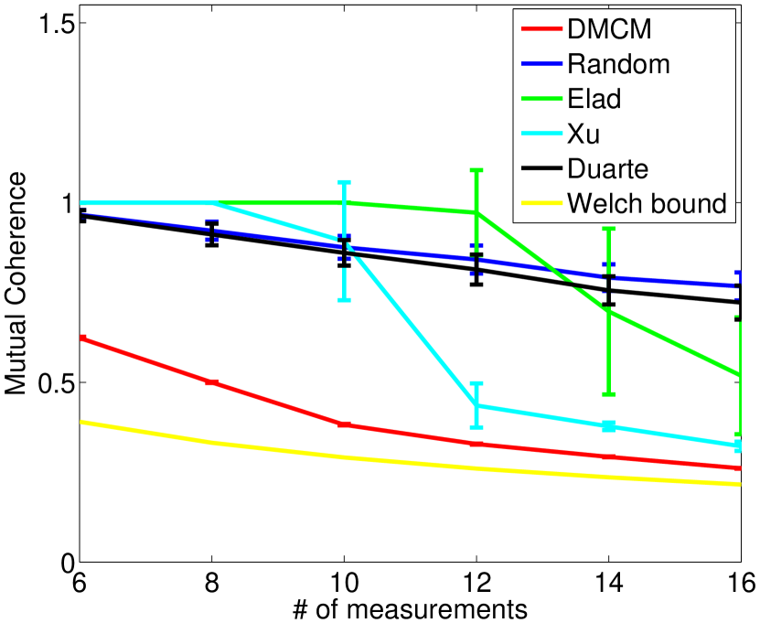
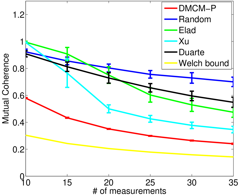
The compared methods are tested on three settings with different sizes of $\mathbf{M}\in\mathbb{R}^{m\times n}$: (1) $m=[6:2:16],n=60$; (2) $m=[10:5:35],n=120$; and (3) $m=[10:10:50],n=180$. Note that the constructed matrices may not be the same for the compared methods with different initializations. So for each choice of size $(m,n)$, we repeat the experiment for 100 times and record the means and standard deviations of the mutual coherences of the constructed matrices $\mathbf{M}$. The means and standard deviations of mutual coherences v.s. the number $m$ of measurements are shown in Figure 1. It can be seen that the matrix constructed by our DMCM achieves much lower mutual coherences than previous methods do. The main reason is that our DMCM minimizes the mutual coherence of $\mathbf{M}$ directly, while the objectives of all the previous methods are indirect. It can also be seen that the standard deviations of our method is close to zero, while some other compared methods may not be stable in some cases. A possible reason is that the solver of our method has convergence guarantee, while other methods do not.

Figure 3: Plots of the means and standard deviations of mutual coherences of $\mathbf{P}\mathbf{D}$ v.s. the number $m$ of measurements, where the elements of $\mathbf{D}$ are uniformly distributed in $[0,1]$.

Table 1: Comparison of running time (in seconds) of DMCM-P, Elad, Xu and Duarte on problem (23) under different settings.

	DMCM-P	Elad	Xu	Duarte
$m=10$, $d=30$, $n=60$	181	5	5	0.0033
$m=20$, $d=60$, $n=120$	582	8	8	0.004
$m=30$, $d=90$, $n=180$	838	14	12	0.004

For the second experiment in this subsection, we show that for given $\mathbf{D}\in\mathbb{R}^{d\times n}$ our DMCM-P is able to compute a projection $\mathbf{P}\in\mathbb{R}^{m\times d}$ such that $\mathbf{P}\mathbf{D}\in\mathbb{R}^{m\times n}$ has low mutual coherence. We choose $\mathbf{D}$ to be a Gaussian random matrix in this experiment. To solve our DMCM-P model in (23), we run Algorithm 4 for 15 iterations and Algorithm 3 for 1000 iterations. In Algorithm 4, we set $\rho_{0}=0.5$, $\beta=2$ and $\eta=1.2$. $\mathbf{P}$ is initialized as a Gaussian random matrix.

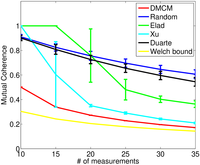
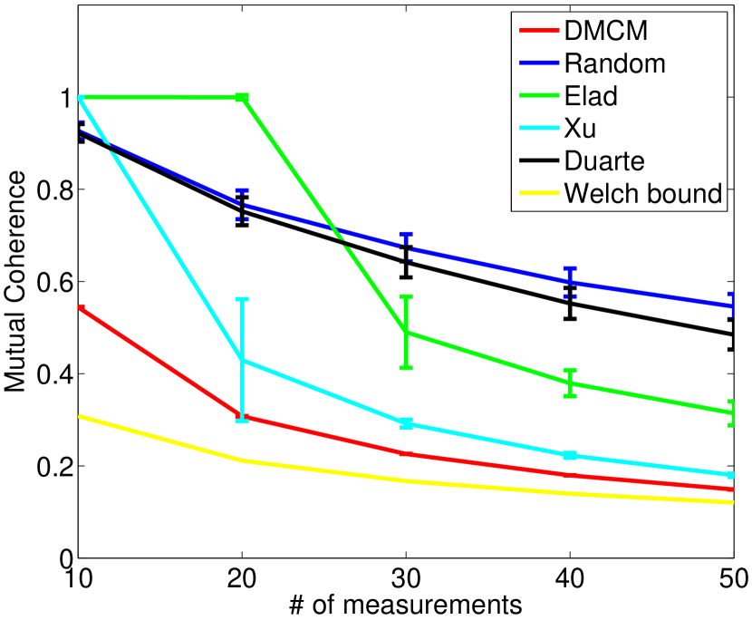
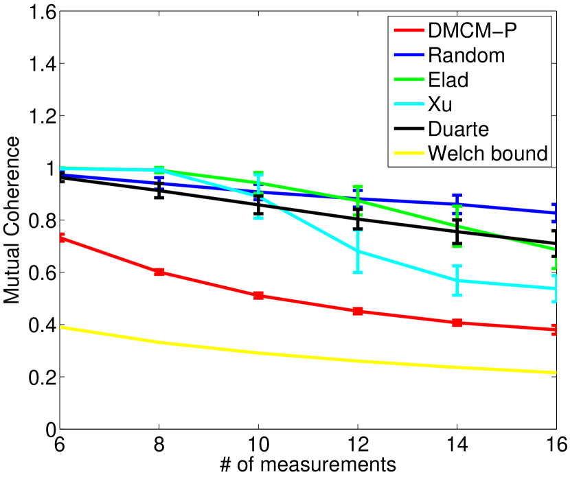
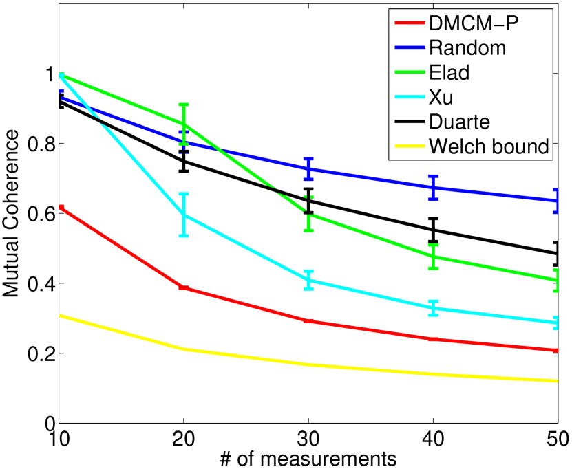
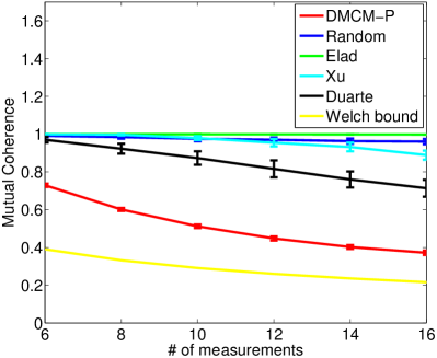
We compare our DMCM-P with the algorithms of Elad [9], Xu et al. [10] and Duarte-Carajalino and Sapiro [12] on the mutual coherence of $\mathbf{P}\mathbf{D}$. We test on three settings: (1) $m=[6:2:16]$, $n=60$, $d=30$; (2) $m=[10:5:35]$, $n=120$, $d=60$; and (3) $m=[10:10:50]$, $n=180$, $d=90$. Figure 2 shows the mutual coherence of $\mathbf{P}\mathbf{D}$ as a function of the number $m$ of measurements. It can be seen that our DMCM-P achieves the best projection such that $\mathbf{P}\mathbf{D}$ has the lowest mutual coherences in all the three settings. So are the standard deviations. Note that our algorithm does not use any special property of $\mathbf{D}$. So it is expected to work for $\mathbf{D}$ in other distributions as well. We test our method in the case that the elements of $\mathbf{D}$ are uniformly distributed in $[0,1]$ and report the results in Figure 3. It can be seen that our method still outperforms other methods in both mean and standard deviation.

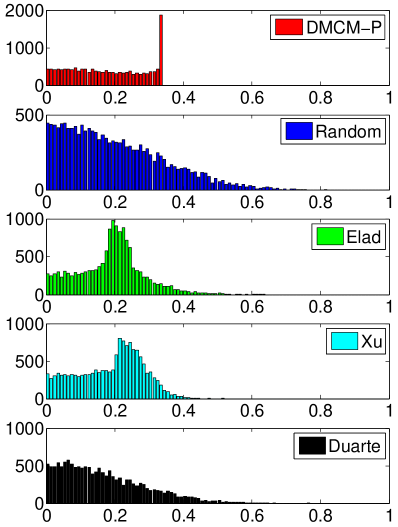
Furthermore, Figure 4 shows the distribution of the absolute values of inner products between distinct columns of $\mathbf{P}\mathbf{D}$ with $m=20$, $n=120$, and $d=60$. It can be seen that our DMCM-P has the shortest tail, showing that the number of elements in the Gram matrix that are closer to the ideal Welch bound is larger than the compared methods. Such a result is consistent with the lowest mutual coherences shown in Figure 2.

Figure 4: Distributions of the absolute values of $(\mathbf{P}\mathbf{D})^{T}(\mathbf{P}\mathbf{D})$.

Finally, we report the running time of the algorithms of Elad, Xu, Duarte and our DMCM-P in Table 1. The settings of the algorithms are the same as those in Figure 2 and the running time is reported based on different choices of $m$, $d$ and $n$. It can be seen that Duarte is the fastest method since it has a closed form solution. Our DMCM-P is not very efficient since we use the continuation trick in Algorithm 4, which repeats Algorithm 3 many times. Note that speeding up the algorithm, although valuable, is not the main focus of this paper. Actually, for many applications the projection matrix $\mathbf{P}$ can be computed offline. So we leave the speeding-up issue as future work.

4.2 Comparing the CS Performance

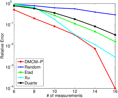
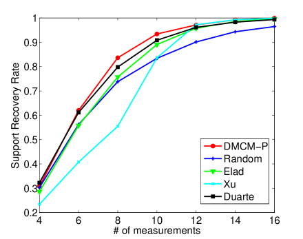
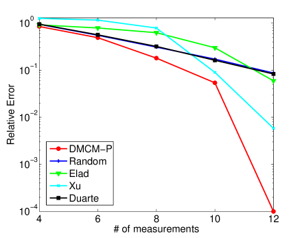
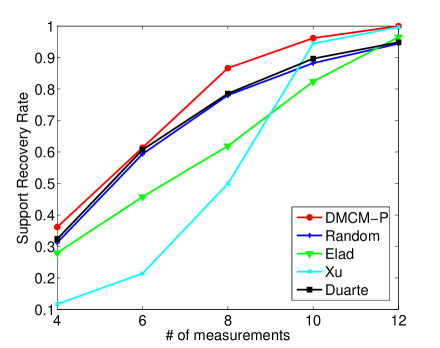
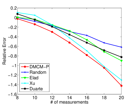
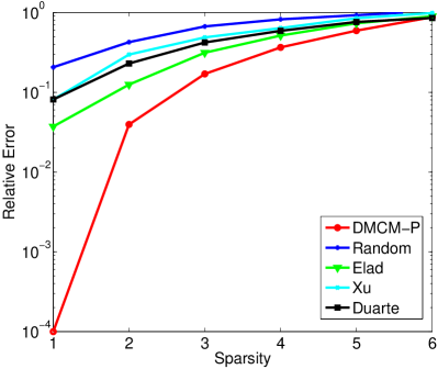
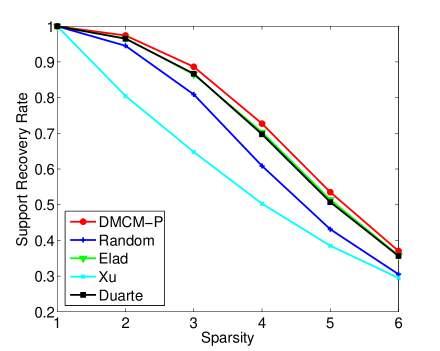
In this subsection, we apply the optimized projection by our DMCM-P to CS. We first generate a $T$-sparse vector $\bm{\alpha}\in\mathbb{R}^{n}$, which constitutes a sparse representation of signal $\mathbf{x}=\mathbf{D}\bm{\alpha}$, where $\mathbf{x}\in\mathbb{R}^{d}$. The locations of nonzeros are chosen randomly and their values obey a uniform distribution in $[-1,1]$. We choose the dictionary $\mathbf{D}\in\mathbb{R}^{d\times n}$ as a Gaussian random matrix, the DCT matrix and the matrix learned by K-SVD, respectively. Then we apply different projection matrices $\mathbf{P}$ learned by our DMCM-P, random projection matrix, and the algorithms of Elad [9], Xu et al. [10] and Duarte-Carajalino and Sapiro [12] to generate the compressed $\mathbf{y}$ via $\mathbf{y}=\mathbf{P}\mathbf{D}\bm{\alpha}$. At last, we solve problem (5) by OMP to obtain $\hat{\bm{\alpha}}$. We compare the performance of projection matrices computed by different methods using the relative reconstruction error $\|\mathbf{x}-\mathbf{x}^{*}\|_{2}/\|\mathbf{x}^{*}\|_{2}$ and the support recovery rate $|\mbox{support}(\mathbf{x})\cap\mbox{support}(\mathbf{x}^{*})|/|\mbox{support}(\mathbf{x}^{*})|$, where $\mathbf{x}^{*}$ is the ground truth. A smaller reconstruction error and larger support recovery rate mean better CS performance.

We conduct two experiments in this subsection. The first one changes the number $m$ of measurements and the second one changes the sparsity level $T$. For every value of the aforementioned parameters we perform 3000 experiments and calculate the average relative reconstruction error and support recovery rate.

Figure 5: Signal reconstruction errors and support recovery rate v.s. number of measurements, where $\mathbf{D}$ is the Gaussian random matrix.

Figure 6: Signal reconstruction error and support recovery rate v.s. number of measurements, where $\mathbf{D}$ is the DCT matrix.

Figure 7: Signal reconstruction error and support recovery rate v.s. number of measurements, where $\mathbf{D}$ is learned by K-SVD.

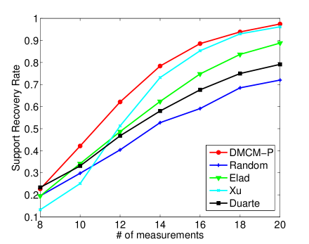In the first experiment, we vary $m$ and set $n=60$, $d=30$, $T=2$ when $\mathbf{D}$ is the Gaussian random matrix, $n=60$, $d=60$, $T=2$ when $\mathbf{D}$ is the DCT matrix and $n=100$, $d=100$, $T=4$ when $\mathbf{D}$ is the matrix learned by K-SVD, respectively. Figure 5, 6 and 7 show the average relative reconstruction error (left) and support recovery rate (right) v.s. the number $m$ of measurements ($T$ is fixed). In the last case, we follow [24] to train a dictionary for sparsely representing patches of size 10$\times$10 extracted from the image Barbara. This image is of size 512$\times$512 and thus has 253009 possible patches, considering all overlaps. We extract one tenth of these patches (uniformly spread) to train on using the K-SVD with 50 iterations. The CS performance improves as $m$ increases. Also, as expected, all the optimized projection matrices produce better CS performance than the random projection does, and our proposed DMCM-P consistently outperforms the algorithms of Elad, Xu et al. and Duarte-Carajalino and Sapiro.

Figure 8: Signal reconstruction error and support recovery rate v.s. sparsity, where $\mathbf{D}$ is the Gaussian random matrix.

Figure 9: Signal reconstruction error and support recovery rate v.s. sparsity, where $\mathbf{D}$ is the DCT matrix.

Figure 10: Signal reconstruction error and support recovery rate v.s. sparsity, where $\mathbf{D}$ is learned by K-SVD.

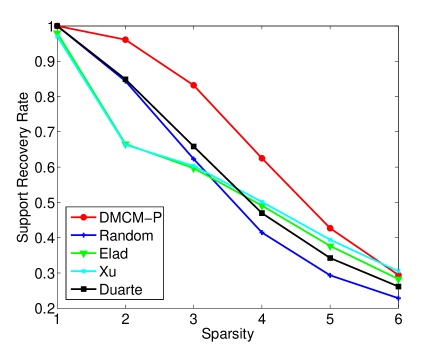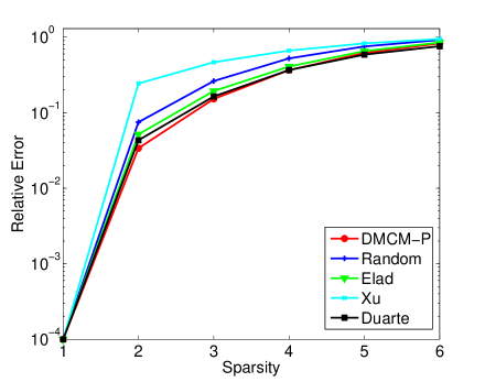
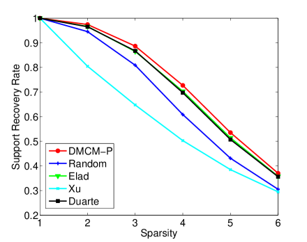
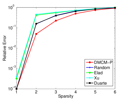
In the second experiment, we vary the sparsity level $T$ and set $m=18$, $n=180$ and $d=90$ when $\mathbf{D}$ is the Gaussian random matrix, $m=15$, $n=180$ and $d=180$ when $\mathbf{D}$ is the DCT matrix and $m=12$, $n=100$ and $d=100$ when $\mathbf{D}$ is the matrix learned by K-SVD. Figure 8, 9 and 10 show the average relative reconstruction error and support recovery rate as a function of the sparsity level $T$ ($m$ is fixed). The CS performance also improves as $T$ decreases. Also, our DMCM-P consistently outperforms random projection and other deterministic projection optimization methods. This is due to the low mutual coherence of $\mathbf{P}\mathbf{D}$ thanks to our optimized projection method as verified in the previous experiments.

Figure 11: Signal reconstruction error and support recovery rate v.s. measurement in the noisy case, where $\mathbf{D}$ is the Gaussian random matrix.

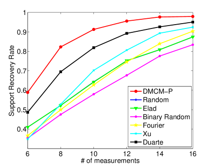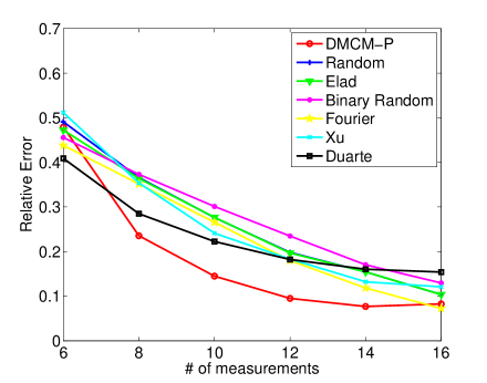
We also test the noisy case. We add Gaussian random noise with 0 mean and 0.01 variance to each element of the observation $\mathbf{y}$ and then recover the true signal from this noisy $\mathbf{y}$. This time we test with $\mathbf{D}$ in another different distribution and another choice of the ratio $n/d$. We generate elements of $\mathbf{D}$ by a uniform distribution on [0,1]. We choose $m=[6:2:16]$, $d=40$ and $n=60$. Besides the sensing matrices constructed via optimization, we also compare DMCM-P with the the random binary matrix and Fourier matrix with random selected rows. Figure 11 shows the performance comparison based on the relative reconstruction error and support recovery rate v.s. the number of measurements. It can be seen that our method also achieves the best performance in almost all cases. The improvement of our method over the random sensing matrices (using Fourier matrix with random selected rows or the random binary matrices) are significant.

5 Conclusions

This paper focuses on optimizing the projection matrix in CS for reconstructing signals which are sparse in some overcomplete dictionary. We develop the first model which aims to find a projection $\mathbf{P}$ by minimizing the mutual coherence of $\mathbf{P}\mathbf{D}$ directly. We solve the nonconvex problem by alternating minimization and prove the convergence. Simulation results show that our method does achieve much lower mutual coherence of $\mathbf{P}\mathbf{D}$, and also leads to better CS performance. Considering that mutual coherence is important in many applications besides CS, we expect that the proposed construction will be useful in many other applications as well, besides CS.

There is some interesting future work. First, though we give the first solver with convergence guarantee in Algorithm 1 for (16), the obtained solution is not guaranteed to be globally optimal due to the nonconvexity of the problem. It is interesting to investigate when the obtained solution is globally optimal. Second, currently the proposed method is not efficient, and it is valuable to find faster solvers. For example, we may consider solving (16) and (22) by Alternating Direction Method of Multiplier (ADMM) after introducing some auxiliary variables, which may be more efficient than our current solvers. But proving its convergence for nonconvex problems, (16) and (22), will be challenging.

Appendix

In this section, we give the proof of Theorem 3.

Definition 2

[25, 26] Let $g$ be a proper and lower semicontinuous function.

1. For a given $\mathbf{x}\in\text{dom}\ g$, the Frechét subdifferential of $g$ at $\mathbf{x}$, written as $\hat{\partial}g(\mathbf{x})$, is the set of all vectors $\mathbf{u}\in\mathbb{R}^{n}$ which satisfies

   $$\liminf_{\mathbf{y}\neq\mathbf{x},\mathbf{y}\rightarrow\mathbf{x}}\frac{g(\mathbf{y})-g(\mathbf{x})-\left\langle\mathbf{u},\mathbf{y}-\mathbf{x}\right\rangle}{\|\mathbf{y}-\mathbf{x}\|}\geq 0.$$

2. The limiting-subdifferential, or simply the subdifferential, of $g$ at $\mathbf{x}\in\mathbb{R}^{n}$, written as $\partial g(\mathbf{x})$, is defined through the following closure process

   $$\partial g(\mathbf{x}) := \{\mathbf{u}\in\mathbb{R}^{n}:\exists\mathbf{x}_{k}\rightarrow\mathbf{x},g(\mathbf{x}_{k})\rightarrow g(\mathbf{x}),$$

   $$\mathbf{u}_{k}\in\hat{\partial}g(\mathbf{x}_{k})\rightarrow\mathbf{u},k\rightarrow\infty\}.$$

Proposition 1

[25, 26] The following results hold:

1. In the nonsmooth context, the Fermat’s rule remains unchanged: If $\mathbf{x}\in\mathbb{R}^{n}$ is a local minimizer of $g$, then $0\in\partial g(\mathbf{x})$.

2. Let $(\mathbf{x}_{k},\mathbf{u}_{k})$ be a sequence such that $\mathbf{x}_{k}\rightarrow\mathbf{x}$, $\mathbf{u}_{k}\rightarrow\mathbf{u}$, $g(\mathbf{x}_{k})\rightarrow g(\mathbf{x})$ and $\mathbf{u}_{k}\in\partial g(\mathbf{x}_{k})$. Then $\mathbf{u}\in\partial g(\mathbf{x})$.

3. If $f$ is a continuously differentiable function, then $\partial(f+g)(\mathbf{x})=\nabla f(\mathbf{x})+\partial g(\mathbf{x})$.

Proof of Theorem 3: First, (25) can be rewritten as

$$\mathbf{M}_{k+1}$$

$$= \arg\min_{\mathbf{M}}\langle\nabla f_{\rho}(\mathbf{M}_{k}),\mathbf{M}-\mathbf{M}_{k}\rangle+\frac{1}{2\alpha}\left\lVert\mathbf{M}-\mathbf{M}_{k}\right\rVert_{F}^{2}$$

$$+\frac{1}{2\beta}\|\mathbf{M}-\mathbf{P}_{k}\mathbf{D}\|_{F}^{2}+h(\mathbf{M}).$$

By the optimality of $\mathbf{M}_{k+1}$, we have

$$h(\mathbf{M}_{k+1})+\left\langle\nabla f_{\rho}(\mathbf{M}_{k}),\mathbf{M}_{k+1}-\mathbf{M}_{k}\right\rangle$$

$$+\frac{1}{2\alpha}\|\mathbf{M}_{k+1}-\mathbf{M}_{k}\|_{F}^{2}+\frac{1}{2\beta}\|\mathbf{M}_{k+1}-\mathbf{P}_{k}\mathbf{D}\|_{F}^{2}$$

$$\leq h(\mathbf{M}_{k})+\frac{1}{2\beta}\|\mathbf{M}_{k}-\mathbf{P}_{k}\mathbf{D}\|_{F}^{2}.$$ (31)

From the Lipschitz continuity of $\nabla f_{\rho}(\mathbf{M})$, we have

$$F(\mathbf{M}_{k+1},\mathbf{P}_{k})$$

$$= f_{\rho}(\mathbf{M}_{k+1})+\frac{1}{2\beta}\|\mathbf{M}_{k+1}-\mathbf{P}_{k}\mathbf{D}\|_{F}^{2}$$

$$\leq f_{\rho}(\mathbf{M}_{k})+\left\langle\nabla f_{\rho}(\mathbf{M}_{k}),\mathbf{M}_{k+1}-\mathbf{M}_{k}\right\rangle$$ (32)

$$+\frac{1}{2\rho}\|\mathbf{M}_{k+1}-\mathbf{M}_{k}\|_{F}^{2}+\frac{1}{2\beta}\|\mathbf{M}_{k+1}-\mathbf{P}_{k}\mathbf{D}\|_{F}^{2}.$$

Add (31) and (32), we have

$$h(\mathbf{M}_{k+1})+F(\mathbf{M}_{k+1},\mathbf{P}_{k})$$

$$\leq h(\mathbf{M}_{k})+f_{\rho}(\mathbf{M}_{k})-\left(\frac{1}{2\alpha}-\frac{1}{2\rho}\right)\|\mathbf{M}_{k+1}-\mathbf{M}_{k}\|_{F}^{2}$$

$$+\frac{1}{2\beta}\|\mathbf{M}_{k}-\mathbf{P}_{k}\mathbf{D}\|_{F}^{2}$$ (33)

$$= h(\mathbf{M}_{k})+F(\mathbf{M}_{k},\mathbf{P}_{k})-\left(\frac{1}{2\alpha}-\frac{1}{2\rho}\right)\|\mathbf{M}_{k+1}-\mathbf{M}_{k}\|_{F}^{2}.$$

Note that $F(\mathbf{M}_{k+1},\mathbf{P})=\frac{1}{2\beta}\|\mathbf{M}_{k+1}-\mathbf{P}\mathbf{D}\|_{F}^{2}$ is $\frac{1}{\beta}\sigma_{\min}^{2}(\mathbf{D})$-strongly convex, where $\sigma_{\min}(\mathbf{D})$ denotes the smallest singular value of $\mathbf{D}$ and it is positive since $\mathbf{D}$ is of full rank. Then by Lemma B.5 in [27] and the optimality of $\mathbf{P}_{k+1}$ to (26), we have

$$F(\mathbf{M}_{k+1},\mathbf{P}_{k+1})\leq F(\mathbf{M}_{k+1},\mathbf{P}_{k})-\frac{1}{2\beta}\sigma_{\min}^{2}(\mathbf{D})\left\lVert\mathbf{P}_{k+1}-\mathbf{P}_{k}\right\rVert_{F}^{2}.$$ (34)

Combining (33) and (34) leads to

$$h(\mathbf{M}_{k+1})+F(\mathbf{M}_{k+1},\mathbf{P}_{k+1})$$

$$\leq h(\mathbf{M}_{k})+F(\mathbf{M}_{k},\mathbf{P}_{k})-\left(\frac{1}{2\alpha}-\frac{1}{2\rho}\right)\|\mathbf{M}_{k+1}-\mathbf{M}_{k}\|_{F}^{2}-\frac{1}{2\beta}\sigma_{\min}^{2}(\mathbf{D})\left\lVert\mathbf{P}_{k+1}-\mathbf{P}_{k}\right\rVert_{F}^{2}.$$ (35)

Second, by the optimality of $\mathbf{M}_{k+1}$, we have

$$0\in \partial h(\mathbf{M}_{k+1})+\nabla f_{\rho}(\mathbf{M}_{k})+\frac{1}{\alpha}(\mathbf{M}_{k+1}-\mathbf{M}_{k})$$

$$+\frac{1}{\beta}(\mathbf{M}_{k+1}-\mathbf{P}_{k}\mathbf{D}).$$ (36)

Thus, there exists $\mathbf{W}_{k+1}\in\nabla_{\mathbf{M}}F(\mathbf{M}_{k+1},\mathbf{P}_{k+1})+\partial h(\mathbf{M}_{k+1})$, such that

$$\mathbf{W}_{k+1}\in \nabla f_{\rho}(\mathbf{M}_{k+1})+\frac{1}{\beta}(\mathbf{M}_{k+1}-\mathbf{P}_{k+1}\mathbf{D})+\partial h(\mathbf{M}_{k+1})$$

$$= \nabla f_{\rho}(\mathbf{M}_{k})+\frac{1}{\beta}(\mathbf{M}_{k+1}-\mathbf{P}_{k}\mathbf{D})+\partial h(\mathbf{M}_{k+1})$$ (37)

$$+(f_{\rho}(\mathbf{M}_{k+1})-f_{\rho}(\mathbf{M}_{k}))+\frac{1}{\beta}(\mathbf{P}_{k}-\mathbf{P}_{k+1})\mathbf{D}.$$

Then, combining (36) and (37) leads to

$$\left\lVert\mathbf{W}_{k+1}\right\rVert_{F}\leq \left\lVert\nabla f_{\rho}(\mathbf{M}_{k})+\frac{1}{\beta}(\mathbf{M}_{k+1}-\mathbf{P}_{k}\mathbf{D})+\partial h(\mathbf{M}_{k+1})\right\rVert_{F}$$

$$+\left\lVert f_{\rho}(\mathbf{M}_{k+1})-f_{\rho}(\mathbf{M}_{k})\right\rVert_{F}+\frac{1}{\beta}\left\lVert(\mathbf{P}_{k}-\mathbf{P}_{k+1})\mathbf{D}\right\rVert_{F}$$ (38)

$$\leq \frac{1}{\alpha}\left\lVert\mathbf{M}_{k+1}-\mathbf{M}_{k}\right\rVert_{F}+\frac{1}{\rho}\left\lVert\mathbf{M}_{k+1}-\mathbf{M}_{k}\right\rVert_{F}+\frac{1}{\beta}\left\lVert\mathbf{D}\right\rVert^{2}\left\lVert\mathbf{P}_{k}-\mathbf{P}_{k+1}\right\rVert_{F},$$ (39)

where (39) uses the property that $\nabla f_{\rho}(\mathbf{M})$ is Lipschitz continuous with the Lipschitz constant $1/\rho$. Also, by the optimality of $\mathbf{P}_{k+1}$, we have

$$\mathbf{0}=\nabla_{\mathbf{P}}F(\mathbf{M}_{k+1},\mathbf{P}_{k+1})=(\mathbf{M}_{k+1}-\mathbf{P}_{k+1}\mathbf{D})\mathbf{D}^{T}.$$ (40)

Third, note that $F(\mathbf{M},\mathbf{P})$ is coercive, i.e., $F(\mathbf{M},\mathbf{P})$ is bounded from below and $F(\mathbf{M},\mathbf{P})\rightarrow+\infty$ when $\|[\mathbf{M},\mathbf{P}]\|_{F}\rightarrow+\infty$. It can be seen from (35) that $F(\mathbf{M}_{k},\mathbf{P}_{k})$ is bounded. Thus $\{\mathbf{M}_{k},\mathbf{P}_{k}\}$ is bounded. Then there exists an accumulation point $(\mathbf{M}^{*},\mathbf{P}^{*})$ and a subsequence $\{\mathbf{M}_{k_{j}},\mathbf{P}_{k_{j}}\}$ such that $(\mathbf{M}_{k_{j}},\mathbf{P}_{k_{j}})\rightarrow(\mathbf{M}^{*},\mathbf{P}^{*})$ as $j\rightarrow+\infty$. Since $F(\mathbf{M},\mathbf{P})$ is continuously differentiable, we have $F(\mathbf{M}_{k_{j}},\mathbf{P}_{k_{j}})\rightarrow F(\mathbf{M}^{*},\mathbf{P}^{*})$. As $h(\mathbf{M}_{k})=0$ for all $k$ and the set $\{\mathbf{M}:\|\mathbf{M}_{i}\|_{2}=1,i=1,\cdots,n\}$ is closed, we have $h(\mathbf{M}^{*})=0$ and $F(\mathbf{M}_{k_{j}},\mathbf{P}_{k_{j}})+h(\mathbf{M}_{k_{j}})\rightarrow F(\mathbf{M}^{*},\mathbf{P}^{*})+h(\mathbf{M}^{*})$.

$\hfill\blacksquare$

Reference

References

- [1] E. J. Candès, J. Romberg, T. Tao, Robust uncertainty principles: Exact signal reconstruction from highly incomplete frequency information, IEEE Transactions on Information Theory 52 (2) (2006) 489–509.
- [2] D. L. Donoho, Compressed sensing, IEEE Transactions on Information Theory 52 (4) (2006) 1289–1306.
- [3] B. K. Natarajan, Sparse approximate solutions to linear systems, SIAM Journal on Computing 24 (2) (1995) 227–234.
- [4] S. S. Chen, D. L. Donoho, M. A. Saunders, Atomic decomposition by basis pursuit, SIAM Journal on Scientific Computing 20 (1) (1998) 33–61.
- [5] Y. C. Pati, R. Rezaiifar, P. Krishnaprasad, Orthogonal matching pursuit: Recursive function approximation with applications to wavelet decomposition, in: Signals, Systems and Computers, 1993. 1993 Conference Record of The Twenty-Seventh Asilomar Conference on, IEEE, 1993, pp. 40–44.
- [6] R. Gribonval, M. Nielsen, Sparse representations in unions of bases, IEEE Transactions on Information Theory 49 (12) (2003) 3320–3325.
- [7] D. L. Donoho, M. Elad, Optimally sparse representation in general (nonorthogonal) dictionaries via minimization, Proceedings of the National Academy of Sciences 100 (5) (2003) 2197–2202.
- [8] J. A. Tropp, Greed is good: Algorithmic results for sparse approximation, IEEE Transactions on Information Theory 50 (10) (2004) 2231–2242.
- [9] M. Elad, Optimized projections for compressed sensing, IEEE Transactions on Signal Processing 55 (12) (2007) 5695–5702.
- [10] J. Xu, Y. Pi, Z. Cao, Optimized projection matrix for compressive sensing, EURASIP Journal on Advances in Signal Processing 2010 (2010) 43.
- [11] E. J. Candes, T. Tao, Near-optimal signal recovery from random projections: Universal encoding strategies?, IEEE Transactions on Information Theory 52 (12) (2006) 5406–5425.
- [12] J. M. Duarte-Carvajalino, G. Sapiro, Learning to sense sparse signals: Simultaneous sensing matrix and sparsifying dictionary optimization, IEEE Transactions on Image Processing 18 (7) (2009) 1395–1408.
- [13] L. Welch, Lower bounds on the maximum cross correlation of signals (corresp.), IEEE Transactions on Information theory (1974) 397–399.
- [14] C. Bao, Y. Quan, H. Ji, A convergent incoherent dictionary learning algorithm for sparse coding, in: European Conference on Computer Vision, Springer, 2014, pp. 302–316.
- [15] D. Barchiesi, M. D. Plumbley, Learning incoherent dictionaries for sparse approximation using iterative projections and rotations, IEEE Transactions on Signal Processing 61 (8) (2013) 2055–2065.
- [16] B. Li, Y. Shen, J. Li, Dictionaries construction using alternating projection method in compressive sensing, IEEE Signal Processing Letters 18 (11) (2011) 663–666.
- [17] K. Schnass, P. Vandergheynst, Dictionary preconditioning for greedy algorithms, IEEE Transactions on Signal Processing 56 (5) (2008) 1994–2002.
- [18] Y. Nesterov, Smooth minimization of non-smooth functions, Mathematical Programming 103 (1) (2005) 127–152.
- [19] Y. S. John Duchi, Shai Shalev-Shwartz, T. Chandra, Efficient projections onto the -ball for learning in high dimensions, in: International Conference of Machine Learning, 2008.
- [20] H. Attouch, J. Bolte, B. F. Svaiter, Convergence of descent methods for semi-algebraic and tame problems: proximal algorithms, forward–backward splitting, and regularized gauss–seidel methods, Mathematical Programming 137 (1-2) (2013) 91–129.
- [21] H. Rauhut, Compressive sensing and structured random matrices, Theoretical foundations and numerical methods for sparse recovery 9 (2010) 1–92.
- [22] E. Candes, J. Romberg, Sparsity and incoherence in compressive sampling, Inverse problems 23 (3) (2007) 969.
- [23] G. Puy, P. Vandergheynst, Y. Wiaux, On variable density compressive sampling, IEEE Signal Processing Letters 18 (10) (2011) 595–598.
- [24] M. Eald, Sparse and redundant representations: From theory to applications in signal and image processing, Springer.
- [25] R. R. Tyrrell, W. Roger (Eds.), Variational Analysis, Springer, 1998.
- [26] S. S. Jérôme Bolte, M. Teboullez, Proximal alternating linearized minimization for nonconvex and nonsmooth problems, Mathematical Programming 146 (1-2) (2014) 459–494.
- [27] J. Mairal, Optimization with first-order surrogate functions, in: International Conference on Machine Learning, 2013, pp. 783–791.