How does noise affect the structure of a chaotic attractor: A recurrence network perspective

Abstract

We undertake a preliminary numerical investigation to understand how the addition of white and colored noise to a time series affects the topology and structure of the underlying chaotic attractor. We use the methods and measures of recurrence networks generated from the time series for this analysis. We explicitly show that the addition of noise destroys the recurrence of trajectory points in the phase space. By using the results obtained from this analysis, we go on to analyse the light curves from a dominant black hole system and show that the recurrence network measures are effective in the analysis of real world data involving noise and are capable of identifying the nature of noise contamination in a time series.

1 Introduction

It is now well known that many time evolutions in Nature are inherently governed by nonlinear dynamical systems. For a proper understanding of these time evolutions, one often resorts to the methods and tools of nonlinear time series analysis [1], since the information regarding the system in most cases is available in the form of a time series. There are two important properties that are the hallmarks of every dynamical system - determinism and recurrence. The former implies that the future behavior of the system can be accurately predicted, given sufficient knowledge of the current state of the system. By the latter property, the trajectory of a dynamical system tends to revisit every region of the phase space over an interval of time [2]. Hence, these two properties are very important in nonlinear analysis of time series data. Of special interest, in the analysis, is the search for deterministic chaos in the time evolution of the system and the presence of an underlying chaotic attractor. Because of this, many quantifiers from chaos theory [3, 4] are constantly being employed in the nonlinear analysis of observational data.

The single largest problem in the time series analysis of real data is the presence of noise, both white and colored, that tend to destroy both the above mentioned properties of any dynamical system underlying the time series. Several aspects of the effect of noise on synthetic as well as real world data and on the quantifying measures of discrimination have been addressed by many authors since the advent of chaos theory some four decades back. For example, the influence of white noise on the logistic attractor [5], the effect of colored noise on chaotic systems [6], method to distinguish chaos from colored noise in an observed time series [7] and the seminal work on the correlation dimension analysis of colored noise data by Osborne and Provenzale [8], to mention a few. The above studies resulted in the development of surrogate methods [9, 10] to discriminate chaos from random noise in real world data. More details on the effect of noise on chaotic systems and discriminating measures can be found in several standard books on chaos [1, 3, 4].

In this paper, we apply the newly emerged tool of recurrence networks (RN) and the related measures [11, 12] to undertake a preliminary numerical analysis to show how a chaotic attractor is affected by white and colored noise. The basic idea of RN analysis is that the information inherent in a chaotic time series is mapped onto the domain of a complex network using a suitable scheme. One then uses the statistical measures of the complex network to characterize the underlying chaotic attractor in the time series. There are two aspects of the RN that make them special for the analysis of time series data. Firstly, since the network measures can be derived from a small number of nodes in the network, the method is suitable for the analysis of short, non stationary data [13]. Secondly, the type of RN called the $\epsilon$ - RNs (whose details are given in the next section) that we consider in this work, generally preserve the topology of the embedded attractor from the time series [14]. We show this specifically for the standard Lorenz attractor below. Hence, the topological changes in the underlying attractor due to noise addition are also reflected in the corresponding RN. This, in turn, implies that the RN and measures can be effectively used to study how the topological structure of a chaotic attractor is affected by increasing levels of noise contamination.

Figure 1: The RP generated from the standard Lorenz attractor time series.

Figure 2: Variation of the count of disuade nodes as a function of $\epsilon$ for the RNs constructed with $M=3$ from random and Lorenz attractor time series for $N=2000$ and $5000$.

The above properties of the RN have resulted in a number of practical appliations ranging from identification of dynamical transitions in model systems and real data [15, 16] to classification of cardio vascular time series [17]. However, there is one area where the RN measures have not been tested properly. For example, a systematic analysis of how the RN measures change with the addition of noise and how effective these measures are in the analysis of real data involving noise, are missing. To our knowledge, there is only one related study by Thiel et al. [18] using recurrence plot (RP) measures in this regard. These factors motivate us for the present analysis.

It should be noted that our aim in this analysis is neither to quantify the amount of noise in a given time series nor to distinguish deterministic nonlinear behavior from randomness in a given time series using any quantifying measure from RN. We focus on the following two aspects:

i) How the contamination of white and colored noise affect the topological structure of a low dimensional chaotic attractor?

ii) How effective are the RN measures in the analysis of real world data containing noise?

We introduce an additional measure for this purpose derived from the RN, which we call the k-spectrum. Also, we use the time series from the standard Lorenz attractor as the prototype to study the effect of noise on synthetic data. The analysis is done by adding different amounts of white and colored noise to the Lorenz data. The results obtained from this is used for the analysis of real world data.

Our paper is organised as follows: In the next section, we discuss the details regarding all the numerical tools used in this analysis, namely, the RP and the RN and the associated measures. In §3, we use the time series from the standard Lorenz attractor as an example to construct the RN and study how the network measures change by the addition of different amounts of white and colored noise. The §4 is devoted to the analysis of a few light curves from a standard black hole system GRS 1915+105 which are expected to contain different levels of white and colored noise. Conclusions are given in §5.

Figure 3: The figure shows the construction of the RN from a time series. The top panel shows the Lorenz attractor time series and the embedded attractor from it using the time delay. The bottom panel shows the RN constructed from the embedded attractor and the corresponding k-spectrum (see text).

Figure 4: The left panel shows the time series and the RN of the Lorenz attractor with number of nodes $N=2000$. The right panel shows the k-spectrum and the degree distribution derived from the RN. Note that the variation in the degree of each node and its position in the RN can be clearly seen from the colour gradient for $k$.

2 Numerical Tools: RP and RN

In this section, we provide details of all the quantifying measures used for this study. RP is a visualisation tool introduced by Eckmann et al. [2]. It is a two dimensional graphical representation of the trajectory of the dynamical system in the form of a binary, symmetric matrix $\mathcal{R}$ where $R_{ij}$ = 1 if the state $\vec{x_{j}}$ is a neighbour of $\vec{x_{i}}$ in phase space and $R_{ij}=0$, otherwise. The neighbourhood is defined through a certain recurrence threshold $\epsilon$. To construct the RP from a scalar time series $s(1),s(2),.....s(N_{T})$, the time series is first embedded in $M$-dimensional space using the time delay co-ordinates [19] using a suitable time delay $\tau$, where $N_{T}$ is the total number of points in the time series. The procedure creates delay vectors in the embedded space of dimension $M$ given by

$$\vec{x_{i}}=[s(i),s(i+\tau),......s(i+(M-1)\tau)]$$ (1)

There are a total number of $N=N_{T}-(M-1)\tau$ vector points in the reconstructed space representing the attractor. Any point $\jmath$ on the attractor is considered to be in the neighbourhood of a reference point $\imath$ if their distance in the $M$-dimensional space is less than the threshold $\epsilon$. Thus we have

$$R_{ij}=H(\epsilon-||\vec{x_{i}}-\vec{x_{j}}||)$$ (2)

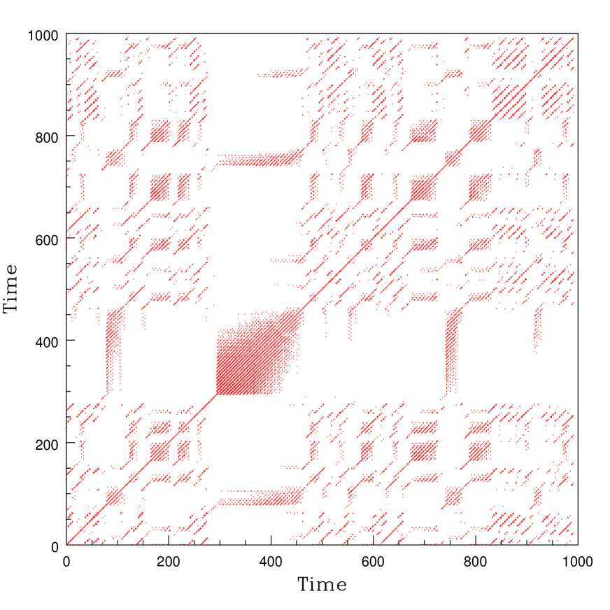
where $H$ is the Heaviside function and $||..||$ is a suitable norm. Here we use the Euclidean norm. As an example, the RP constructed from the standard Lorenz attractor time series is shown in Fig. 1.

The RP has become more popular with the introduction of the recurrence quantification analysis (RQA) [20, 21] that uses the quantifying measures derived from the RP for the analysis of the data. For example, two important measures that are commonly used are the recurrence rate (RR) and the determinism (DET) given by

$$RR={{1}\over{N^{2}}}\sum_{i,j}R_{ij}$$ (3)

$$DET={{\sum_{l\geq l_{min}}^{l_{max}}lp(l)}\over{\sum_{l=1}^{l_{max}}lp(l)}}$$ (4)

The former is a measure of the overall probability that a certain state recurs while the latter is a measure based on the distribution of the diagonal structures $p(l)$ and reflects how predictable the system is. Here we use DET as a quantifying measure in our analysis.

Figure 5: The time series, RN, k-spectrum and the degree distribution for a pure random time series.

Figure 6: Same as the previous figure for the red noise. Note that the range of the k-spectrum is much large compared to the RN of both random and Lorenz attractor and the topology of the RN is similar to that of a typical chaotic attractor.

The measures based on complex networks have emerged as a popular tool for the analysis of dynamical systems, especially in the form of time series, in the last two decades. The advantage of this approach is that one is able to extract information regarding the topological properties of the underlying attractor, which are otherwise unable to get, using conventional nonlinear time series analysis. The networks based on recurrence are called proximity networks which are mainly of two class, the fixed mass (or k-nearest neighbour) networks [22, 23] and the fixed volume (or $\epsilon$ - recurrence) networks [13, 14]. In the former, the neighburhood of a trajectory point for recurrence is defined in terms of fixed number of nearest neighbours while in the latter it is defined in terms of fixed phase space volume. In this paper, we use the procedure based on the $\epsilon$ - RN for the construction of networks from time series, confining to the case of unweighted $\epsilon$ - RN.

The generation of $\epsilon$ - RN (which, from now on, we simply call RN) is closely associated with the RP. Infact, the adjacency matrix $\mathcal{A}$ for the unweighted RN can be obtained by removing the identity matrix from the recurrence matrix defined above:

$$A_{ij}=R_{ij}-\delta_{ij}$$ (5)

where $\delta_{ij}$ is the Kronecker delta. Note that, once the adjacency matrix is defined, the time series has been converted into a complex network. Each point on the embedded attractor is taken as a node and it is connected to every other node whose distance is $\leq\epsilon$. The binary adjacency matrix contains 1 for all the pairs of points on the attractor that satisfy the condition $||\vec{x_{i}}-\vec{x_{j}}||\leq\epsilon$ and zero otherwise.

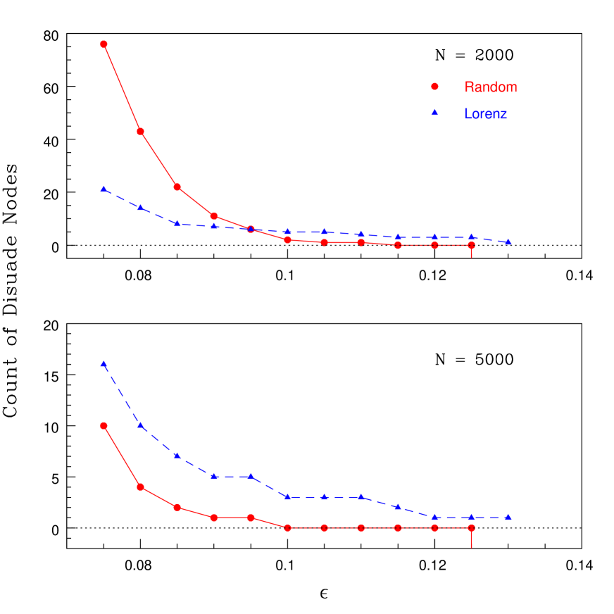
The two important parameters associated with the RN construction from time series are the threshold $\epsilon$ and the embedding dimension $M$. In this paper, we do the analysis by choosing $M=3$. For the selection of the critical threshold $\epsilon_{c}$ for RN construction, we closely follow the methods adopted by Donges et al. [24] and Eroglu et al. [25]. The basic criterion employed is that the RN should appear as a giant cluster with the number of disuade (disconnected) nodes negligible compared to $N$. In order to get a non subjective comparison of $\epsilon_{c}$ between different systems, we first transform the time series into a uniform deviate so that the size of the embedded attractor is rescaled into the unit interval $[0,1]$. The RN is constructed from the time series for $M=3$ taking a range of $\epsilon$ values from $0.02$ to $0.2$. We then compute the count of disuade nodes in the RN as a function of $\epsilon$. The results are shown in Fig. 2 for random and Lorenz attractor time series for $N=2000$ and $5000$. Note that a giant cluster appears for both systems with $<0.5\%$ disuade nodes corresponding to $\epsilon\sim 0.1$ for $N=2000$. For $N=5000$, this critical value of $\epsilon$ gets slightly decreased. Hence we use $\epsilon_{c}\equiv 0.1$ as the critical threshold for construction of RN in this paper.

Figure 7: The RP constructed from the Lorenz attractor time series by adding four different percentages of white noise: $(a)4\%(SNR=25)$, $(b)10\%(SNR=10)$, $(c)20\%(SNR=5)$ and $(d)50\%(SNR=2)$. Note that the structure of the Lorenz attractor, as reflected in the RP, is not completely lost untill the SNR becomes 2.

Figure 8: Same as the previous figure, but using red noise instead of white noise. As in the previous case, only when the noise level reaches $50\%$, the RP loses the characteristic features of the Lorenz attractor.

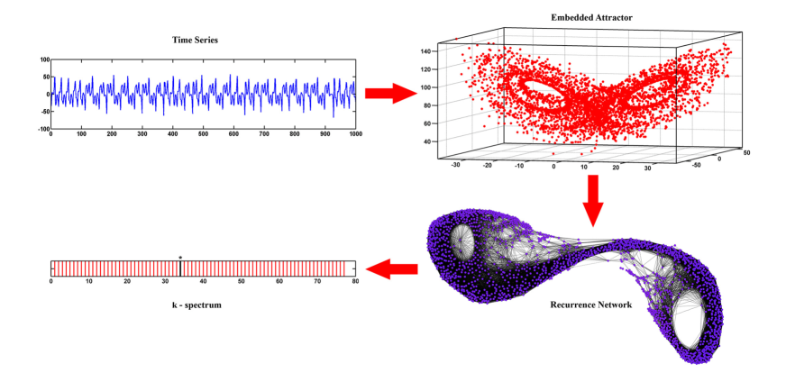
As an example, we show in Fig. 3 the construction of the RN from the Lorenz attractor time series. We use the Gephi software $(https://gephi.org/)$ for all the graphical representations of the network in this paper. Note that, by the nature of the network construction, the topology of the embedded attractor is preserved in the RN. Each point on the attractor has become a node in the RN and the number of nodes connected to a reference node is known by its degree denoted by $k$. We show below that the range of $k$ - values can represent the topological changes of the attractor due to noise addition and hence we use this as an additional measure, called the $k$ - spectrum, in this paper. It is also shown in Fig. 3 for the RN from the Lorenz attractor.

The other important characteristic measures from RN used in this analysis are the degree distribution, the characteristic path length (CPL) and the average clustering coefficient (CC). The degree distribution indicates how many nodes $n_{k}$ among the total number of nodes $N$ have a given degree $k$. It is usually represented as a probability distribution $P(k)$ as a function of $k$, where $P(k)={{n_{k}}\over{N}}$. For random networks, $P(k)$ tends to be a Poisson distribution for large $N$. The CPL, denoted by $<l>$, is defined through the shortest path $l_{s}$ connecting two nodes $\imath$ and $\jmath$. For unweighted and undirected networks that we consider in this work, $l_{s}$ is defined as the minimum number of nodes to be traversed to reach from $\imath$ to $\jmath$. The average value of $l_{s}$ for all the pair of nodes in the whole network is defined as $<l>$ and the maximum value of $l_{s}$ is taken as the diameter of the network. The CPL can be computed from the equation

$$<l>={{1}\over{N(N-1)}}\sum_{i,j}^{N}l_{s}$$ (6)

The CC of the network is defined through a local clustering index $c_{v}$. Its value is obtained by counting the actual number of edges in a sub graph with respect to node $v$ as reference to the maximum possible edges in the sub graph:

$$c_{v}={{\sum_{i,j}A_{vi}A_{ij}A_{jv}}\over{k_{v}(k_{v}-1)}}$$ (7)

The average value of $c_{v}$ is taken as the CC of the whole network:

$$CC={{1}\over{N}}\sum_{v}c_{v}$$ (8)

For a detailed discussion of all the network measures, see the popular books by Newman [26] and Watts [27] and some excellent reviews on the subject [28, 29].

Figure 9: The figure shows how the k-spectrum of the RN constructed from a chaotic attractor varies by adding different percentages of white noise to the time series from the attractor. It is clear that the white noise affects the nodes with high degrees or hubs reducing their links so that the network tends to a random network as noise level increases.

Figure 10: The degree distribution for the RNs constructed from Lorenz attractor time series by adding different percentages of white noise. The degree distribution approaches Poissonian as the noise level increases.

3 Analysis of Synthetic Data

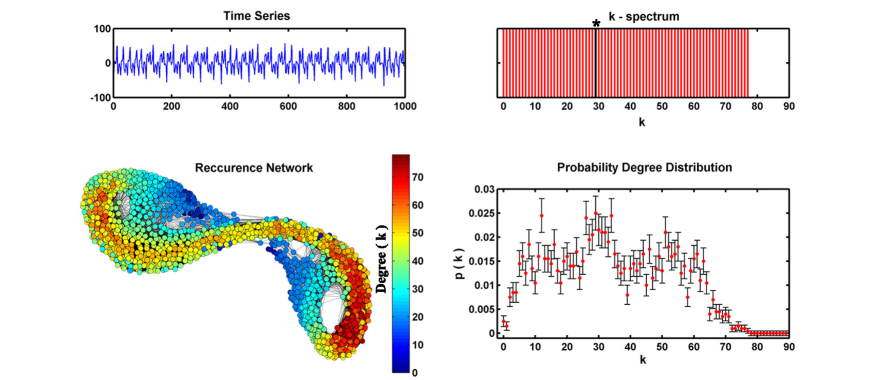
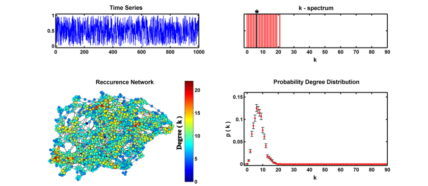
In this section, we study the changes in the topological structure of a chaotic attractor using the RN measures by the addition of different percentages of white and colored noise to the attractor time series. We use the time series from the standard Lorenz attractor for this analysis. The number of nodes in the RN is adjusted to be $N=2000$ for all computations in this section. In Fig. 4, we show the Lorenz attractor time series and the constructed RN on the left side, where as, the $k$ - spectrum and the degree distribution computed from the RN are shown on the right side. The colour gradient is an indication of how the $k$ value changes over the attractor. Note that the range of the $k$ - spectrum is from 1 to 78. A star over a perticular $k$ value in the spectrum indicates that this $k$ value is the most probable or the maximum number of nodes in the RN have this degree. It corresponds to the largest peak in the degree distribution shown below the $k$ - spectrum. The error bar in the degree distribution is estimated from counting statistics resulting from the finiteness in the number of nodes. The statistical error associated with any counting of $n(k)$ is $\sqrt{n(k)}$. If $n(k)\rightarrow 0$, one typically takes the error to be normalised as 1. Thus, the error associated with $P(k)$ is typically ${{\sqrt{n(k)}}\over{N}}$ and becomes $1/N$ as $n(k)\rightarrow 0$.

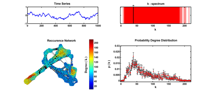
Next, we generate an ensemble of noise data sets, both white and colored. The colored noise are correlated random fractals whose power vary, in general, as ${{1}\over{f^{\alpha}}}$ with the different values of the spectral index $\alpha$ producing different types of colored noise. We use colored noise data sets for $\alpha=1,1.5$ and $2.0$ for the analysis and results are explicitly shown here for one type of colored noise with $\alpha=2.0$, called the red noise. In Fig. 5, we show the time series, RN, $k$ - spectrum and the degree distribution for the white noise and in Fig. 6, that for red noise. Note that both are completely different with respect to the corresponding measures for the Lorenz data. While the RN for white noise does not have a specific structure, that for colored noise has a structure similar to that of a chaotic attractor. As expected, the range of $k$ - spectrum is much smaller for the white noise with the degree distribution tending to a Poissonian, where as, the $k$ - spectrum and distribution of the red noise has a much wider range compared even to that of the RN from Lorenz attractor. We have found that the range of $k$ values in the RN of colored noise increases as the spectral index $\alpha$ increases from 1 to 2, with $\alpha=1$ very close to that of white noise $(\alpha=0)$. This difference in the behavior between white and colored noise can be attributed to the fact that while white noise tend to fill the entire available phase space, the colored noise is a self affine fractal curve which fills only a sub space of the total phase space resulting in a highly clustered structure and a large range of values in the $k$ - spectrum.

Figure 11: The variation of the k-spectrum of the RN constructed from chaotic attractors by adding different levels of red noise to the time series from the attractor. Just like the white noise, the effect of red noise also is to reduce the high degrees in the network, but even with large amount of noise, the k-spectrum does not approach that of pure red noise.

Figure 12: Same as Fig.10, but for red noise addition instead of white noise. As the noise level increases, the degree distribution deviates from that of the Lorenz attractor.

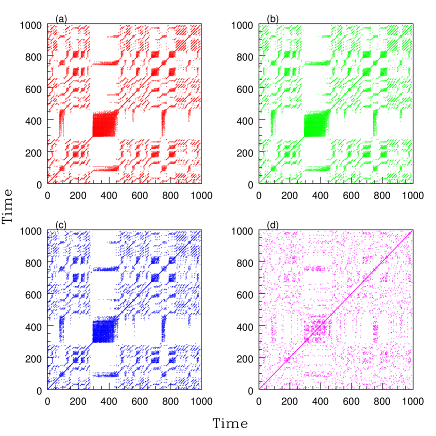
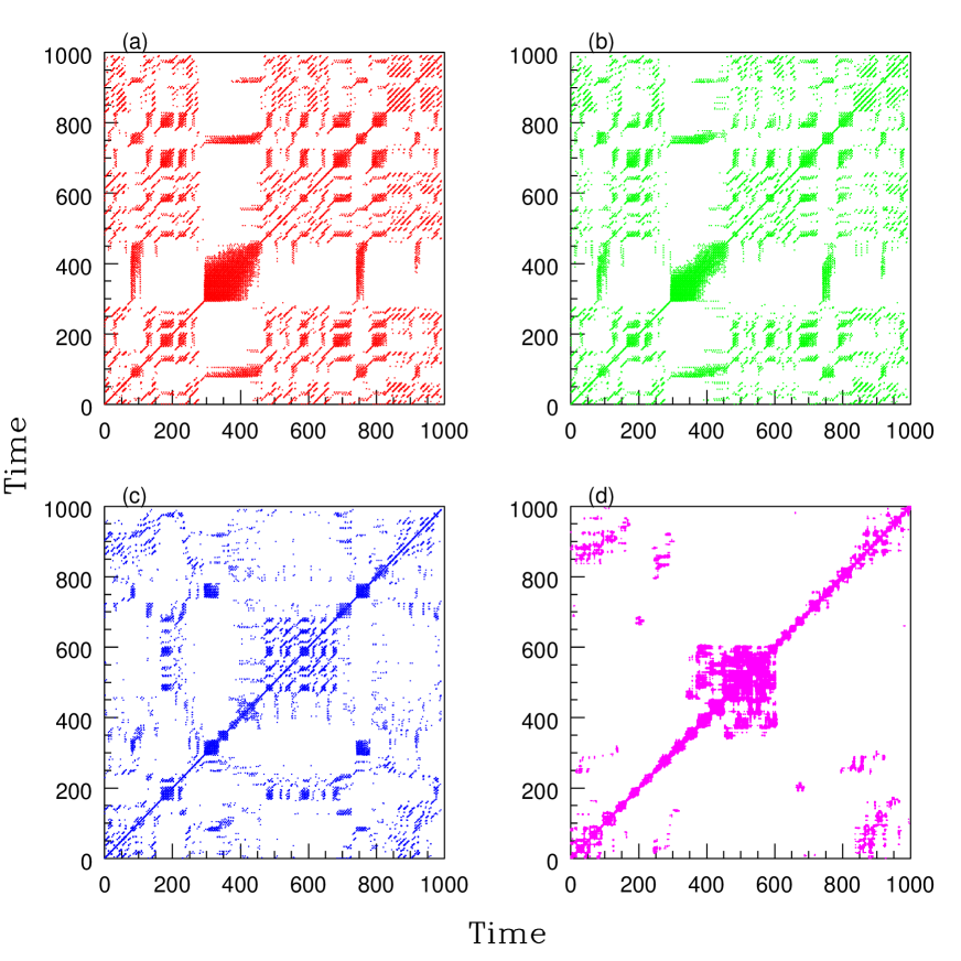
To study the effect of noise contamination, we now add different percentages of each type of noise to the time series from the Lorenz attractor. Here we show the results for noise addition of $5\%$ (SNR 20), $10\%$ (SNR 10), $20\%$ (SNR 5) and $50\%$ (SNR 2). In Fig. 7, we show the RPs generated from time series obtained by adding the above four levels of white noise to the Lorenz data, with the noise level increasing from $(a)$ to $(d)$. A visual inspection shows that only when the noise level reaches $50\%$, the information in the Lorenz attractor is almost completely lost. For the pure Lorenz attractor, the value of $DET$ computed from the RP is $0.988$ while for the pure white noise, it is $0.482$. As the percentage of noise increases, the value of $DET$ decreases as $0.961$ for $5\%$, $0.902$ for $10\%$, $0.814$ for $20\%$ and $0.604$ for $50\%$. The same results for the addition of red noise are shown in Fig. 8. Again, the value of $DET$ decreases as $0.938$ for $5\%$, $0.867$ for $10\%$, $0.768$ for $20\%$ and $0.570$ for $50\%$, with the value for pure red noise as $0.455$. Thus it is found that the time series retains much of the information regarding the attractor even with moderate noise addition of both white and colored noise.

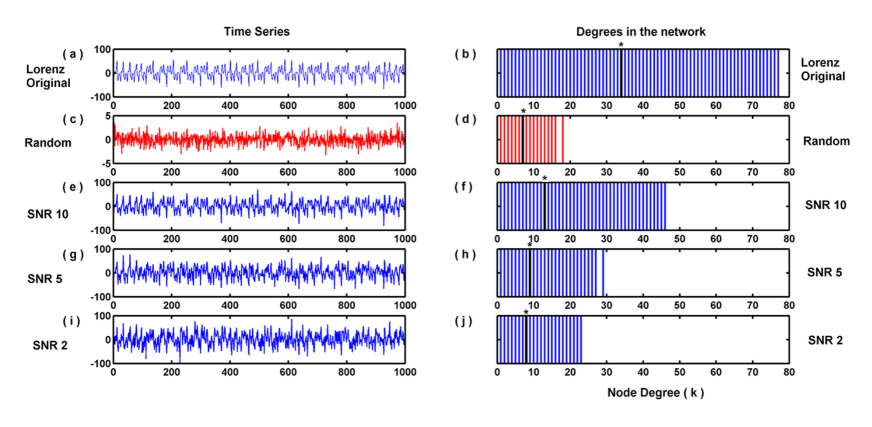
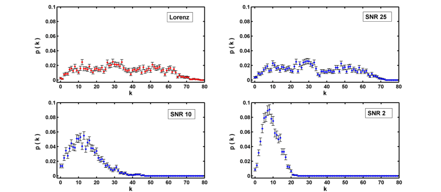
We now study the effect of noise on the various measures of RN. In Fig. 9, we show the original Lorenz time series and white noise along with time series obtained by adding three different percentages of white noise to that of Lorenz on the left panel. The $k$ - spectrum of the corresponding RN are shown on the right panel. It is evident that the addition of white noise affects the nodes with largest degree or hubs in the RN. As the noise level increases, the range of $k$ values keeps on decreasing untill, at sufficiently high noise level, most of the nodes in the RN have $k$ value around the average $<k>$, with the degree distribution tending to Poissonian. This can be more clearly seen from Fig. 10 where, the $P(k)$ versus $k$ for the four RNs in the above case are presented.

Figure 13: The RN and k-spectrum of the Lorenz attractor compared with that of three different attractors obtained by adding different percentages of white noise to the Lorenz attractor time series. As the noise level increases, the maximum k-value keeps on decreasing. The topology of the attractor also approaches that of random.

Figure 14: Same as the previous figure, but for red noise addition instead of white noise. The k-spectrum first decreases and then increases, while the structure changes continuously as red noise content increases.

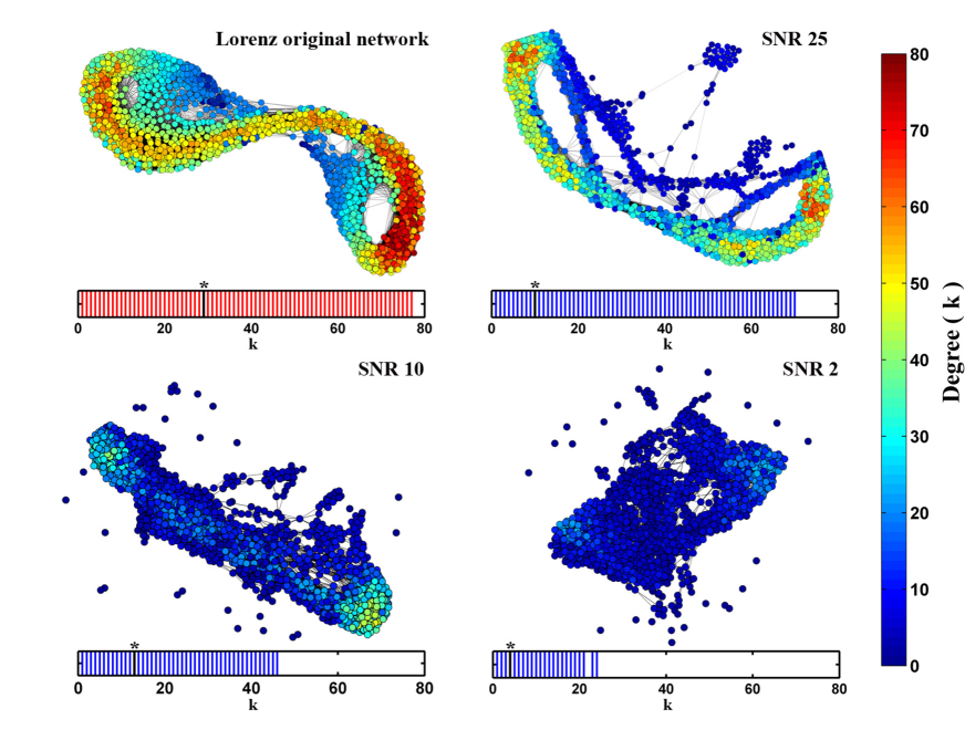
Since the topology of the RN is reflected from that of the actual attractor, this result implies that white noise affects the most clustered or dense regions of the attractor. The noise destroys the recurrence of the trajectory points in the phase space and the trajectory points which are otherwise, tend to be very close over a time interval, become more widely separated. At sufficiently high noise level, the trajectories tend to fill the available phase space completely with approximately equal separation between two trajectory ponts.

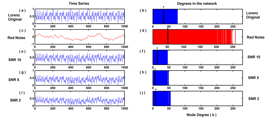
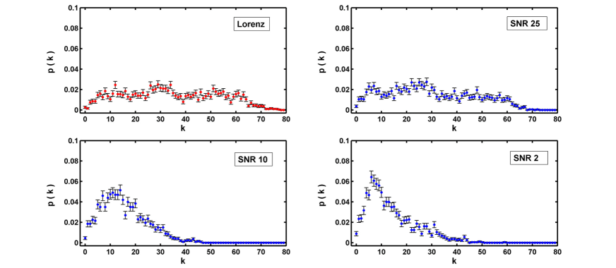
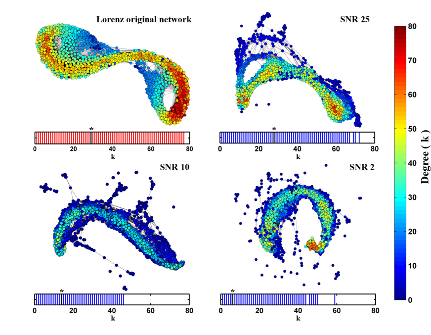
In Fig. 11 and Fig. 12, we show the same results as shown in the previous two figures, but for contamination with the red noise $(\alpha=2.0)$. Now the range of the $k$ - spectrum is set with that of the red noise as the reference. Here again the range of $k$ values gets reduced initially by the addition of colored noise, but tends to increase slowly as the noise level is increased. This trend is also reflected in the degree distribution shown in Fig. 12. However, the effect of colored noise is distinctly different from that of white noise as is evident from the RP shown in Fig. 8. The colored noise also destroys recurrence of the trajectory and the recurrence occurs only around the main diagonal in the RP. This is mainly due to the proximity of the trajectory points in time rather than in space. Thus, every node will only be connected to the nodes closer in time and hence have approximately the same average degree, except a few nodes having comparatively large degree due to confinement and clustering in a lower dimension. This is reflected in the degree distribution shown in Fig. 12. The topological structure of the chaotic attractor in the phase space is also changed accordingly.

To show this explicitly, we present the RN for the orignal Lorenz attractor along with that for time series added with three different levels of white noise and red noise in Fig. 13 and Fig. 14 respectively. The colour grading with respect to the range of $k$ values make the figures self explanatory. Note that, in both cases, the structure of the Lorenz attractor is not completely lost untill the level of noise contamination reaches $50\%$ in agreement with the results obtained from the RPs.

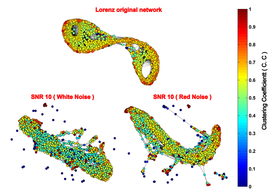
So far we have been using the $k$ - spectrum and the degree distribution to study the effect of noise. It is also important to see how the other network measures vary with the addition of white and colored noise. In Fig. 15, we show how the clustering coefficient of individual nodes $c_{v}$, given by Eq.(7), vary over the RN for three cases, namely, the Lorenz attractor time series and that added with $10\%$ of white and colored noise. It is found that the $c_{v}$ of many nodes decrease by the addition of noise, especially the white noise. This results in a sharp reduction of the average CC of the RN with the addition of white noise.

Figure 15: Variation of the clustering coefficient of the individual nodes $c_{v}$ for the RN of the Lorenz attractor and that for two attractors obtained by adding $10\%$ white noise as well as red noise to the Lorenz attractor time series.

Figure 16: The top panel shows the CPL-CC graph for RN from the Lorenz attractor, attractors obtained by adding different amounts of white noise to the Lorenz attractor time series and RN for random time series.

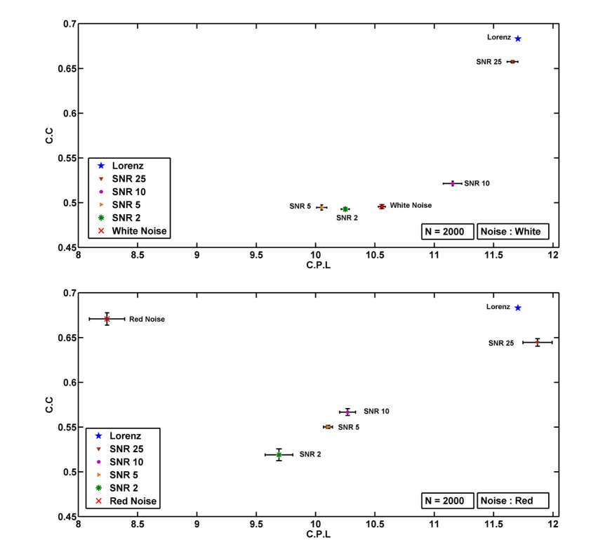
Finally, we show how the CPL and the average CC of the RN vary with noise addition by using a combined plot. For this, we first generate an ensemble of $20$ time series for the Lorenz attractor by changing initial conditions and also $20$ time series each for white and red noise. We then add different percentages of white and red noise to the Lorenz data, generating $20$ ensembles of time series for each noise level. By constructing the RN from each time series, the CPL and CC are computed. The results are plotted on a CPL - CC graph for each type of noise separately. The results are shown in Fig. 16 for both white and red noise. The error bar along the $X$ and $Y$ directions are the standard deviations in the values for CPL and CC respectively from $20$ ensembles in each case.

It is evident that for white noise addition, there is a systematic decrease in the values of both CPL and CC as the $\%$ of noise increases. However, the result of addition of red noise is different. Though CPL and CC generally decrease with noise, the RN from pure red noise appears to behave differently. Its CPL is much less compared to that of all other RNs, but the CC is close to that of the RN from Lorenz attractor. The reason for this is not difficult to understand. We have found that, for the same number of nodes, the $k$ - spectrum and the range of $k$ values for the RN from red noise is much large compared to all other RNs, indicating the presence of some nodes with large degree or hubs. This decreases its CPL significantly. Due to the confinement of the trajectory in a lower dimension resulting in clustering of trajectory points, the average CC remains high.

Figure 17: The light curves from four representative spectroscopic classes of the black hole system GRS 1915+105.

Figure 18: The RPs constructed fom the light curves of the black hole system shown in the previous figure. The states, except kaiA, appears to have some deterministic nonlinear structure mixed with white or colored noise.

4 Aplication to Real World Data

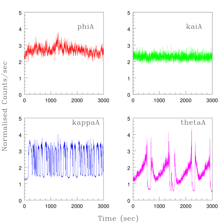
We now check whether the results obtained in the previous section can be used to extract some preliminary information regarding the nature observational data from the real world through the computation of RN measures. Specifically, we use the X-ray light curves from a dominant black hole binary GRS 1915+105 for our analysis. The temporal properties of this black hole system have been classified into $12$ different spectroscopic classes by Belloni et al. [30] based on RXTE observation. The system appears to flip from one state to another randomly in time. Here we have chosen data sets from $4$ out of these $12$ for our analysis, namely, kappaA, kaiA, phiA and thetaA. Each light curve consists of $3200$ continuous data points without any gap. We have already applied surrogate analysis to the light curves from all the $12$ temporal states and have shown that a few of them show deterministic nonlinear behavior [31]. Recently, by combining the results of computations by various quantifiers from conventional nonlinear time series analysis, we were able to group some of these light curves together based on their dynamical behavior [32]. Here we have chosen representative light curves from all these groups for the analysis. These light curves are shown in Fig. 17.

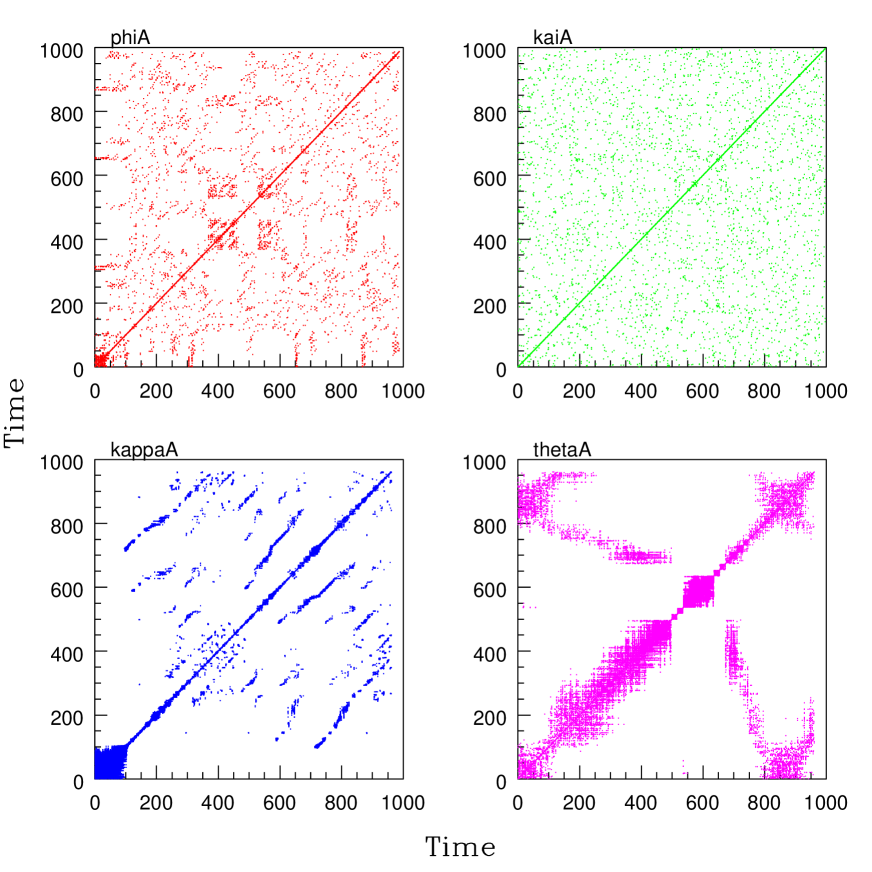
We first compute the RPs from these light curves and they are shown in Fig. 18. The values of $DET$ obtained from the RPs are $0.723,0.502,0.794$ and $0.688$ for phiA, kaiA, kappaA and thetaA respectively. A comparison of the figure with Fig. 7 and Fig. 8 and the values of $DET$ obtained from them tells us that kaiA is close to pure white noise while the other three deviate from pure stochastic behavior. PhiA can be considered to be contaminated with fair amount of white noise and thetaA is mixed with some form of colored noise in high percentage. The bahavior of kappaA suggests that it is a good candidate for deterministic nonlinear behavior added with small amounts of colored noise.

Figure 19: The RN and degree distribution for two of the GRS states that appear to have some nonlinearity mixed with noise.

Figure 20: The CPL-CC values for the RN from the four GRS states along with that for Lorenz attractor, white noise and red noise for comparison.

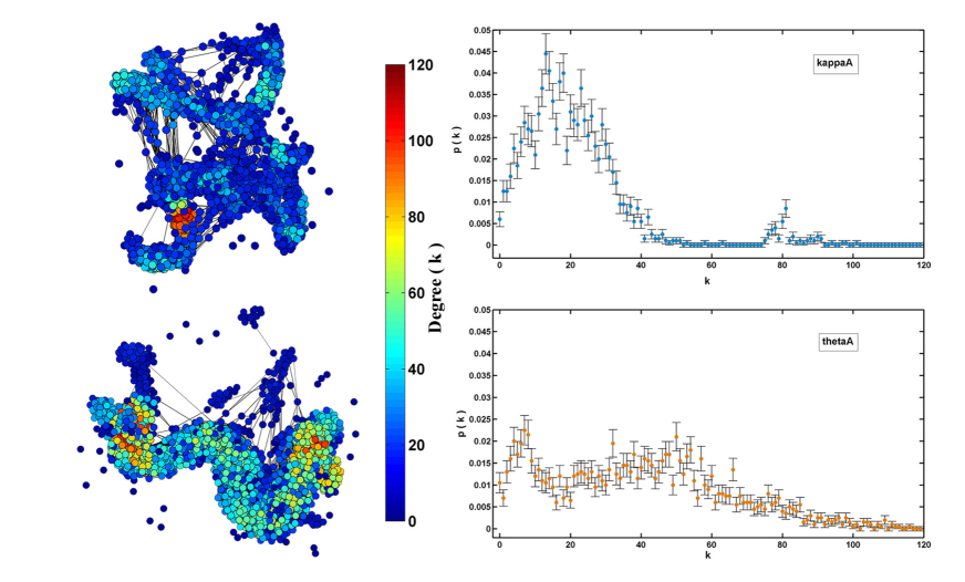
To further validate these results, we now compute the RNs and the associated measures from these light curves. As expected, RN from kaiA coincides almost exactly with that of white noise and RN and distribution of phiA show only small change from that of white noise. However, the RNs from kappaA and thetaA are found to be more interesting. These are shown in Fig. 19 along with the corresponding degree distribution. It is evident that both light curves are contaminated with colored noise and the $\%$ of noise appears to be much more in thetaA compared to kappaA.

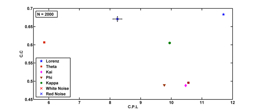
Finally, we look at the CPL - CC plot for the light curves as shown in Fig. 20. For a better comparison, we have added the values for the RNs from the pure Lorenz attractor, white noise and red noise. The position of kaiA almost coincides with that of white noise. While phiA is slightly away indicating high level of white noise, position of thetaA suggests high percentage of colored noise. Only kappaA has least amount of noise contamination with network measures comparatively close to that of Lorenz attractor.

We find that the present analysis has provided us more information regarding the nature of noise content in some light curves compared to our earlier analysis using conventional measures, such as, correlation dimension and entropy [31, 33]. For example, due to high white noise content, phiA was identified as white noise in our earlier analysis. The present analysis shows that it is not. Similarly, the colored noise content in thetaA was not evident in the earlier surrogate analysis. However, our results on kappaA and kaiA remain unchanged from previous analysis. Overall, our numerical analysis shows that the RP and RN measures are capable of detecting noise contamination in an observational data and are especially effective in distinguishing white and colored noise since they change the network measures differently.

5 Conclusion

There are mainly two purposes for the present study which is numerical in nature. On the one hand, our aim is to understand how the addition of white and colored noise to a time series affect the topology and structure of the underlying chaotic attractor with the help of RN and the statistical measures associated with it. An additional measure, called the $k$ - spectrum, is also introduced by us for this purpose. The standard Lorenz attractor time series is used as the prototype for the numerical analysis. The method involves construction of the RN from the time series through the delay embedded attractor. Different amounts of white and colored noise were added to the Lorenz attractor time series and RN constructed. By computing the RN measures, we could show that the addition of white and colored noise affect the structure of the attractor differently. However, both tend to destroy the characteristic property of recurrence of the trajectory points over the attractor. Nevertheless, the characteristic features of the attractor are not completely lost till the noise level reaches close to $50\%$ in both cases.

The second purpose of this study is to understand how effective the RN measures are in a noisy environment for the analysis of time series from the real world. For this, we use representative light curves from different spectroscopic classes of a black hole system GRS 1915+105, where both white and colored noise are expected. We compute the measures by constructing the RN from these light curves and compare them with the corresponding measures of the RNs obtained from the previous analysis with the synthetic data. We show that these measures are effective for a first analysis of the data and, to some extent, can distinguish between contamination of white and colored noise.

Though the RN and the associated measures have found a large number of applications in various fields, to our knowledge, this is the first attempt where these measures are employed to study the effect of noise in real world data. A distinct advantage of RN measures is that they can be applied to short and non stationary time series, such as, astrophysical light curves, physiological signals, etc. Our numerical results obtained here are only preliminary. We suggest that a combined surrogate analysis including conventional measures as well as the network measures, such as, CC and CPL as discriminating statistic, can provide highly accurate results on the nature and amount of noise content in time series from real world.

References

- [1] H. Kantz and T. Schreiber, Nonlinear Time Series Analysis, Cambridge University Press, Cambridge, 2004.
- [2] J. P. Eckmann, S. O. Kamphorst and D. Ruelle, Recurrence plot of dynamical systems, Europhys Letters 5, 973-977, 1987
- [3] R. C. Hilborn, Chaos Nonlinear Dynamics, Oxford University Press, Oxford, 1994.
- [4] J. C. Sprott, Chaos and Time Series Analysis, Oxford Univ. Press, Oxford, 2003.
- [5] G. Mayer-Kress and H. Haken, The influence of noise on the logistic model, J. Stat. Phys. 26, 149–171, 1981.
- [6] S. Radaelli, D. Plewczynski and W. M. Macek, Influence of colored noise on chaotic systems, Phys. Rev. E 66, 035202(R), 2002.
- [7] M. B. Kennel and S. Isabelle, Method to distinguish possible chaos from colored noise, Phys. Rev. A 46, 3111–3118, 1992.
- [8] A. R. Osborne and A. Provenzale, Finite correlation dimension for stochastic systems with power law spectra, Physica D 35, 357–381, 1989.
- [9] T. Schreiber and A. Schmitz, Improved surrogate data for nonlinearity tests, Phys. Rev. Lett. 77, 635–39, 1996.
- [10] T. Schreiber and A. Schmitz, Surrogate time series, Physica D 142, 346–74, 2000.
- [11] N. Marwan, J. F. Donges, Y. Zou, R. V. Donner and J. Kurths, Complex network approach for recurrence analysis of time series, Phys. Lett. A 373, 4246–4254, 2009.
- [12] R. V. Donner, M. Small, J. F. Donges, N. Marwan, Y. Zou, R. Xiang and J. Kurths, Recurrence based time series analysis by means of complex network methods, Int. J. Bif. Chaos 21, 1019–46, 2011.
- [13] R. V. Donner, Y. Zou, J. F. Donges, N. Marwan and J. Kurths, Recurrence networks: A novel paradigm for nonlinear time series analysis, New J. Phys. 12, 033025, 2010.
- [14] R. V. Donner, J. Heitzig, J. F. Donges, Y. Zou, N. Marwan and J. Kurths, The geometry of chaotic dynamics-A complex network perspective, European Phys. J. B 84, 653–672, 2011.
- [15] J. F. Donges, R. V. Donner, K. Rehfeld, N. Marwan, M. H. Trauth and J. Kurths, Identification of dynamical transitions in marine palaeoclimate records by recurrence network analysis, Nonlinear Proc. Geophys. 18, 545–562, 2011.
- [16] Y. Zou, R. V. Donner, J. F. Donges, N. Marwan and J. Kurths, Identifying complex periodic windows in continuous time dynamical systems using recurrence based methods, CHAOS 20, 043130, 2010.
- [17] R. Avila, A. Gapelyuk, N. Marwan, T. Walther, H. Stepan, J. Kurths and N. Wessel, Classification of cardio-vascular time series based on different coupling structures using recurrence network analysis, Philos. T. Roy. Soc. A 371, 20110623, 2013.
- [18] M. Thiel, M. C. Romano, J. Kurths, R. Mencci, E. Allaria and F. T. Arecci, Influence of observational noise on the recurrence quantification analysis, Physica D 171, 138–152, 2002.
- [19] P. Grassberger and I. Procaccia, Measuring the strangeness of strange attractors, Physica D 9, 189–208, 1983.
- [20] N. Marwan, M. C. Romano, M. Thiel and J. Kurths, Recurrence plot for the analysis of complex systems, Phys. Reports 438, 237–329, 2007.
- [21] S. Schinkel, N. Marwan, O. Dimigen and J. Kurths, Confidence bounds for recurrence based complexity measures, Phys. Lett. A 373, 2245–50, 2009.
- [22] X. Xu, J. Zhang and M. Small, Super family phenomena and motifs of networks induced from time series, Proc. Natl. Acad. Sci. USA 105, 19601–05, 2008.
- [23] M. Small, J. Zhang and X. Xu, Transforming time series into complex networks, Complex Sciences, Springer, pp.2078–89, 2009.
- [24] J. F. Donges, J. Heitzig, R. V. Donner and J. Kurths, Analytical framework for recurrence network analysis of time series, Phys. Rev. E 85, 046105, 2012.
- [25] D. Eroglu, N. Marwan, S. Prasad and J. Kurths, Finding recurrence networks threshold adaptively for a specific time series, Nonlin. Processes Geophys. 21, 1085-1092, 2014.
- [26] M. E. J. Newman, Networks: An Introduction, Oxford Univ. Press, Oxford, 2010.
- [27] D. J. Watts, Six Degrees: The Science of a Connected Age, Norton, New York, 2003.
- [28] R. Albert and A. L. Barabasi, Statistical Mechanics of Complex Networks, Rev. Mod. Phys. 74, 47–97, 2002.
- [29] S. Boccaletti, V. Latora, Y. Moreno, M. Chavez and D. U. Hwang, Complex Networks: Structure and Dynamics, Phys. Reports 424, 175–308, 2006.
- [30] T. Belloni, M. Klein-Wolt, M. Mendez, M. van der Klis and J. van Paradjis, A model-independent analysis of the variability of GRS 1915+105, Astronomy and Astrophys. 355, 271–290, 2000.
- [31] R. Misra, K. P. Harikrishnan, G. Ambika and A. K. Kembhavi, The nonlinear analysis of the black hole system GRS 1915+105, Astrophys. J. 643, 1114–29, 2006.
- [32] K. P. Harikrishnan, R. Misra and G. Ambika, Nonlinear time series analysis of the light curves from the black hole system GRS 1915+105, Research in Astr. and Astrophys. 11, 71–90, 2011.
- [33] K. P. Harikrishnan, R. Misra and G. Ambika, Combined use of correlation dimension and entropy as discriminating measures for time series analysis, Comm. Nonlinear Sci. Num. Simulations 14, 3608–14, 2009.