Cosmic string loop shapes

Abstract

We analyze the shapes of cosmic string loops found in large-scale simulations of an expanding-universe string network. The simulation does not include gravitational back reaction, but we model that process by smoothing the loop using Lorentzian convolution. We find that loops at formation consist of generally straight segments separated by kinks. We do not see cusps or any cusp-like structure at the scale of the entire loop, although we do see very small regions of string that move with large Lorentz boosts. However, smoothing of the string almost always introduces two cusps on each loop. The smoothing process does not lead to any significant fragmentation of loops that were in non-self-intersecting trajectories before smoothing.

I Introduction

Cosmic strings are microscopically thin, astrophysically long objects which may have formed at early times as a result of phase transitions or brane inflation in superstring theories. See Ref. Vilenkin and Shellard (2000) for a review. In the simple cases to be discussed here, cosmic strings have no vertices or ends, and thus form a “network” consisting only of infinite strings and closed loops.

When cosmic strings intersect each other, they can reconnect. In the case of strings formed by phase transitions in field theory, this reconnection nearly always takes place. But in the case of strings from superstring theory, the strings can pass through each other unchanged, only reconnect with some probability $p$ in the range $10^{-3}$ to 1. When a string reconnects with itself, the result is to emit some portion of the string into a closed loop. Closed loops oscillate, emit gravitational waves, and so eventually decay away.

This process allows the long string network to scale with the expansion of the universe, meaning that any statistical measure of the string network properties with dimension (length)^α goes as $t^{\alpha}$, where $t$ is the the age of the universe. In particular, the density of long strings (length per unit volume) goes as $t^{-2}$, and thus scales as radiation in the radiation era and as matter in the matter era. Scaling means that the energy density of strings is a fixed fraction of the total energy density in the radiation and matter eras. Thus they do not dominate the universe as monopoles would Zeldovich and Khlopov (1978); Preskill (1979), nor do their effects become ever tinier with time in these eras.

The evolution of a cosmic string in flat space is easily described. Let $\mathbf{x}(\sigma,t)$ describe the spatial position of the string at time $t$, and let the parameter $\sigma$ be chosen to parameterize the string energy in units of $\mu$, the energy per unit length of a static string. Then one can show that in this gauge, $\mathbf{x}^{\prime 2}+\dot{\mathbf{x}}^{2}=1$, where prime and dot denote differentiation with respect to $\sigma$ and $t$ respectively. By appropriate choice of starting point for $\sigma$ at different $t$, we can make $\mathbf{x}^{\prime}\cdot\dot{\mathbf{x}}=0$. The equations of motion then become

$$\ddot{\mathbf{x}}(\sigma,t)=\mathbf{x}^{\prime\prime}(\sigma,t)\,.$$ (1)

The general solution can be written

$$\mathbf{x}(\sigma,t)={1\over 2}\left[\mathbf{a}(t-\sigma)+\mathbf{b}(t+\sigma)\right]\,,$$ (2)

where $\mathbf{a}$ and $\mathbf{b}$ are any functions obeying the constraint $|\mathbf{a}^{\prime}|=|\mathbf{b}^{\prime}|=1$. In the expanding universe, the solutions are more complicated, but Eqs. (1,2) are good approximations for loops much smaller than the Hubble size.

Because the functions $\mathbf{a}^{\prime}$ and $\mathbf{b}^{\prime}$ have unit magnitude, they trace out paths on the unit sphere, the so-called Kibble-Turok (KT) sphere. In general, one would expect those paths to intersect Kibble and Turok (1982); Turok (1984); Vachaspati (1987). In particular, in the case of a closed loop observed in its rest frame, the center of gravity of $\mathbf{a}^{\prime}(\sigma)$ and $\mathbf{b}^{\prime}(\sigma)$ lies at the center of the sphere, and so these paths will intersect except in special cases.

At an intersection, where $\mathbf{a}^{\prime}(t-\sigma)=\mathbf{b}^{\prime}(t+\sigma)$, Eq. (2) gives $\mathbf{x}^{\prime}=0$ and $\dot{\mathbf{x}}=1$. Thus the string doubles back on itself at a point which (in the approximation of an infinitely thin string) moves at the speed of light. Such a point is called a cusp Turok (1984). At a cusp, the string core may overlap with itself, leading to the emission of high-energy particles Brandenberger (1987); Mohazzab (1994); Blanco-Pillado and Olum (1999); Olum and Blanco-Pillado (1999). The high Lorentz boost near the cusp may also produce beams of gravitational Vachaspati and Vilenkin (1985); Damour and Vilenkin (2000, 2001) or electromagnetic radiation Vilenkin and Vachaspati (1987); Spergel et al. (1987); Blanco-Pillado and Olum (2001); Cai et al. (2012), and if the string is coupled to other fields it may lead to particle production Srednicki and Theisen (1987); Damour and Vilenkin (1997); Peloso and Sorbo (2003); Sabancilar (2010); Long et al. (2014); Long and Vachaspati (2014). Many suggestions have been made for observable astrophysical signatures coming from cosmic string cusps. It is therefore important to understand the parameters that characterize these kinds of events in a typical cosmic string loop produced in a scaling network of strings.

The above argument applies only if strings are smooth. The usual calculations, in fact, assume that $\mathbf{a}^{\prime\prime}$ and $\mathbf{b}^{\prime\prime}$ are of order $1/L$, where $L$ is the invariant length of the string loop. On the other hand, cosmic strings have kinks: places where the direction of the string changes suddenly due to a previous reconnection. Such discontinuities in $\mathbf{a}^{\prime}$ and $\mathbf{b}^{\prime}$ allow them to jump to different parts of the unit sphere without crossing each other. In such cases, the argument fails, and there may be no cusps. To know whether or not there are cusps, we need to know the shape of the functions $\mathbf{a}$ and $\mathbf{b}$.

A loop is born when a long string reconnects with itself. At this time, the loop consists of structures that were present on the long string from which it formed, plus two kinks from the final reconnection. In the first oscillation, the loop may fragment, but after one oscillation fragmentation is rare. (In flat space, loop trajectories are periodic, so after one whole oscillation without fragmentation, no further fragmentation is possible. In the expanding universe there is a correction, but it is typically small.) After that, the loop slowly loses energy by emitting gravitational waves, with power $\Gamma G\mu^{2}$, where $\Gamma$ is a number of order 50 Vachaspati and Vilenkin (1985); Turok (1984); Burden (1985); Garfinkle and Vachaspati (1987) and $G$ is Newton’s constant. This leads the loop to lose length at rate $\Gamma G\mu$. When it has lost a significant fraction of its length by this process, its shape may be substantially modified. In particular, we expect it to be much smoother than it was at formation.

The loops which are most important for observable signals are those which have significantly evaporated. At any given time $t$ in the history of the universe, most string is in loops of size around $\Gamma G\mu t$, which are thus roughly half evaporated Blanco-Pillado et al. (2014). Even if we consider loops of some fixed size $\ell$, most of these were created long ago Blanco-Pillado et al. (2014) and have suffered significant evaporation, except for those of the very largest sizes.

The goal of this paper is to determine the shape of cosmic string loops over the course of their lives. We start by analyzing loops and long strings taken directly from a large cosmic string network simulation in the expanding universe. We find that these strings consist primarily of long segments that are generally straight, connected by large-angle kinks. The straight segments are not exactly straight, but rather consist of several shorter and straighter segments, with smaller-angle kinks between those. We never see a smooth motion of $\mathbf{a}^{\prime}$ or $\mathbf{b}^{\prime}$ from one place to another of the sort that could lead to the formation of a cusp.

Thus the track of $\mathbf{a}^{\prime}$ or $\mathbf{b}^{\prime}$ in the simulated loops at formation consists not of a smooth, closed curve, as usually envisioned, but rather of a sequence of small, irregular regions. Within each region, the tangent vector jumps rapidly from place to place, and the regions are connected by sudden, large jumps. In a loop, these regions are either well separated or touch along a curve, but they never significantly overlap or cross through each other. Thus the “crossings” of $\mathbf{a}^{\prime}$ and $\mathbf{b}^{\prime}$ occur entirely in the large jumps (kinks) and never in smooth regions of string that would lead to the phenomenology associated with cusps.

Our large scale string network simulation does not include gravitational back reaction, so it is accurate only at scales above those that might be smoothed by that process. But gravitational effects on long strings, and thus on newly formed loops, are not very important. Loops forming at any given time have sizes much larger than $\Gamma G\mu t$ Blanco-Pillado et al. (2011) so their general shapes are little affected by previous smoothing.

Gravitational effects after loop formation, however, are very important, as discussed above. Unfortunately, we are not presently able to simulate the gravitational back-reaction on a loop. So instead, we attempt to understand it by smoothing the loop using convolution, as described below. This gives us a more realistic population of loops with various degrees of smoothing, and we study these in addition to the newborn loops. Indeed, after significant smoothing, most loops have two significant cusps in each oscillation.

The rest of this paper is organized as follows. In the next section, we discuss the shape of loops directly taken from the simulation without gravitational smoothing, and in Sec. III we discuss the structures found on long strings. In Sec. IV we discuss our smoothing procedure, and in Sec. V we discuss the shape of loops with various degrees of smoothing, the number and size of cusps they produce, their distribution of angular momenta, and to what degree the trajectory of each loop lies on a plane. We conclude in Sec. VI.

II Loops at formation

We first discuss the shape of cosmic string loops just as they are found in our simulation, which does not included gravitational smoothing. Our simulation process is described in detail in Refs. Blanco-Pillado et al. (2011, 2012). The results in this section are taken from a simulation in the matter era of size 500 in units of the initial correlation length. The initial conformal time for this simulation is 4.5 and the ending time 500.0, so the dynamic range is 110.

Several groups have studied the properties of non-intersecting loops from a set of random initial conditions Scherrer et al. (1990); Copi and Vachaspati (2011). We will make some comparisons with these other studies when appropriate. On the other hand, our results should describe more accurately the properties of real loops from a network since we take the initial distribution of loops from a scaling network of strings. In fact we believe these loops are a good representative set of scaling loops themselves. (See the discussion in Ref. Blanco-Pillado et al. (2011)).

Because $\mathbf{a}^{\prime}$ and $\mathbf{b}^{\prime}$ are piecewise linear in our simulation, their paths on the unit sphere consist of discrete points corresponding to the linear pieces. Where the string changes direction at a kink, there is a line connecting two points.

In Fig. 1

Figure 1: The paths of $\mathbf{a}^{\prime}$ (red or dark) and $\mathbf{b}^{\prime}$ (blue or light) on the unit sphere for a loop of length 6.28 seen at time 500.0. Each vertex represents a segment with constant tangent vector. The tangent vectors have been projected from the unit sphere into the figure plane with the Mollweide projection (the same one usually used for cosmic microwave background maps). Kinks are represented by straight lines on the figure.

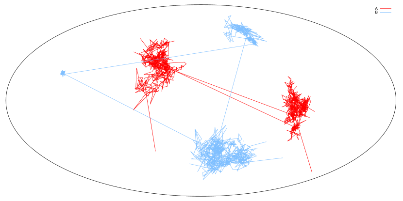
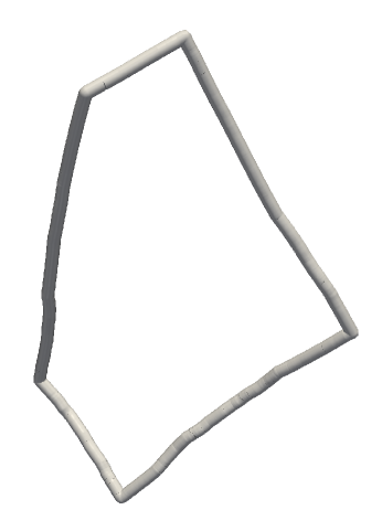
we show the paths of $\mathbf{a}^{\prime}$ and $\mathbf{b}^{\prime}$ for a non-self-intersecting loop appearing in our simulation at time 500. We see immediately that the tangent vectors are arranged in five separated clumps, with jumps between them. In this particular case, the clumps of $\mathbf{a}^{\prime}$ are well separated from the clumps of $\mathbf{b}^{\prime}$. The only places where the paths of $\mathbf{a}^{\prime}$ and $\mathbf{b}^{\prime}$ cross each other are in large-angle kinks that connect the different clumps. Thus this loop will not produce any of the traditional cusps. We show in Fig. 2 a snapshot of this loop in physical space at a time when one can clearly see the five different directions made from these blobs.

Figure 2: A snapshot of the loop represented by its $\mathbf{a}^{\prime}$ and $\mathbf{b}^{\prime}$ in Fig. 1. One can clearly see the 5 different orientations of the tangent vector of the string corresponding the 5 combinations of the regions of $\mathbf{a}^{\prime}$ and $\mathbf{b}^{\prime}$ in the Kibble-Turok sphere in Fig. 1 that exist at this time. The small variations of the tangent vector in each of these segments give some idea of the angular spread of the lumps on the KT sphere.

A more common situation is shown in Fig. 3.

Figure 3: The paths of $\mathbf{a}^{\prime}$ (red or dark) and $\mathbf{b}^{\prime}$ (blue or light) on the unit sphere for a loop of length 8.29.

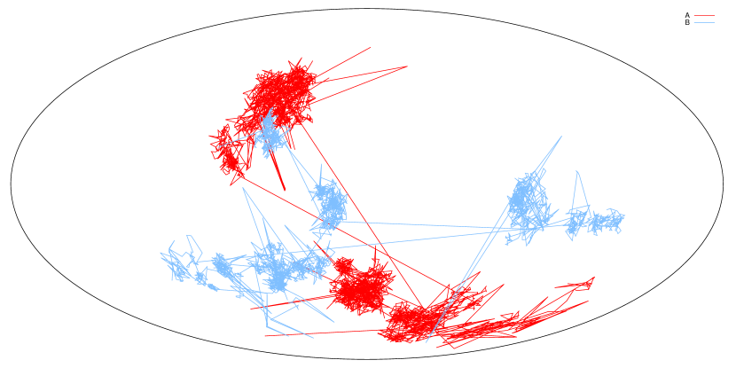
In this case the clumps of $\mathbf{a}^{\prime}$ and $\mathbf{b}^{\prime}$ touch along a curve, further shown in Fig. 4.

Figure 4: Close-up of the upper left of Fig. 3.

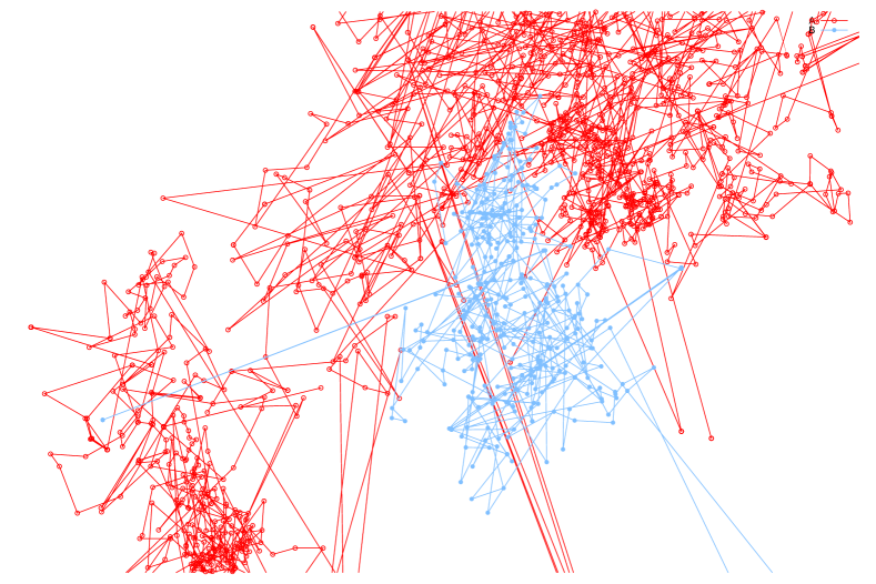
This happens because overlapping segments are lost to loop production, until the unit sphere has been divided into domains with many points of $\mathbf{a}^{\prime}$ and those with many $\mathbf{b}^{\prime}$, separated by a complicated curve. This is the telltale sign of a non-self-intersecting loop on the Kibble-Turok sphere. The non-self-intersecting loops resulting from our simulations cover a continuum of possible distributions of clumps on the sphere, from the kind of well separated clumps in Fig. 1 through the type represented by the first panel in Fig. 9 below, where most of the sphere is covered by the blobs.

One can disturb this situation by introducing additional perturbations to the loops so that the “islands” of $\mathbf{a}^{\prime}$ heavily overlap the ones of $\mathbf{b}^{\prime}$. We have performed such experiments with a number of loops. The result from this exercise is an excited loop whose subsequent evolution quickly produces an important amount of fragmentation until one is back again in a similar representation of the loop on the KT sphere of isolated blobs of $\mathbf{a}^{\prime}$ and $\mathbf{b}^{\prime}$ segments.

Near the dividing curve between the $\mathbf{a}^{\prime}$ and $\mathbf{b}^{\prime}$ clumps, there will be points of $\mathbf{a}^{\prime}$ and points of $\mathbf{b}^{\prime}$ that are very close to each other. In fact, there are even some points that lie on the “wrong side” of this curve, i.e., places where points of $\mathbf{a}^{\prime}$ reach into the domain of $\mathbf{b}^{\prime}$, and vice versa. In most such cases, the distance (angle) on the wrong side of the curve is quite small, but there are a few cases, such as the leftmost point of $\mathbf{a}^{\prime}$ in Fig. 4, where $\mathbf{a}^{\prime}$ reaches deeply into the domain of $\mathbf{b}^{\prime}$. Such deep excursions seem to consist only of single points with only a very tiny amount of string. For example, the point mentioned above represents a segment of $\mathbf{a}^{\prime}$ with length less than $10^{-8}$.

When $\mathbf{a}^{\prime}$ and $\mathbf{b}^{\prime}$ are nearly equal, a piece of string will move rapidly. This may lead to gravitational wave emission and other signatures. In some ways, these regions are similar to cusps. Indeed, they may be an important source of gravitational waves, which will be the subject of a separate paper. However, they do not have the usual form of the cusp where $\mathbf{a}^{\prime}$ and $\mathbf{b}^{\prime}$ move steadily across the sphere and cross each other. They certainly cannot be analyzed by Taylor series expansion around a crossing point, as is usually done for cusps.

III Long strings

We can gain some further insight into the shape of strings by looking at the tangent vectors to the long strings in our simulation. In Fig. 5 we show a section of $\mathbf{a}^{\prime}$ of length 25.9 consisting of 13197 consecutive straight segments of string.

Figure 5: 13197 consecutive segments of a long string at time 500.0, separated into 4 clumps by a hierarchical clustering algorithm. The clumps are shown with different colors (shading) and symbols. Dotted lines show the kinks that connect the clumps.

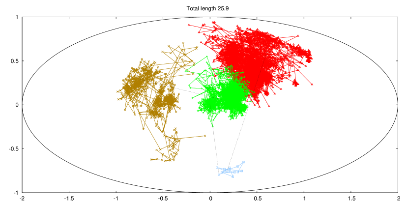
The colors are chosen by a hierarchical clustering algorithm, which works as follows. We first merge the two segments of $\mathbf{a}^{\prime}$ which are the closest on the unit sphere, replacing them by a merged segment with the total length and the average direction. The average is weighted by the length of each segment. We then proceed to the next-closest pair, and so on. When the angle between two pieces of string (which may be the results of previous merges) is greater than a threshold, here $60^{\circ}$, we stop merging.

The clustering procedure has divided the path of $\mathbf{a}^{\prime}$ into 4 “clumps”. Within each clump, the points appear to wander over a certain region of the unit sphere. Large kinks connect each clump to the next.

Figure 6

Figure 6: The leftmost clump of Fig. 5, further broken down with threshold $40^{\circ}$

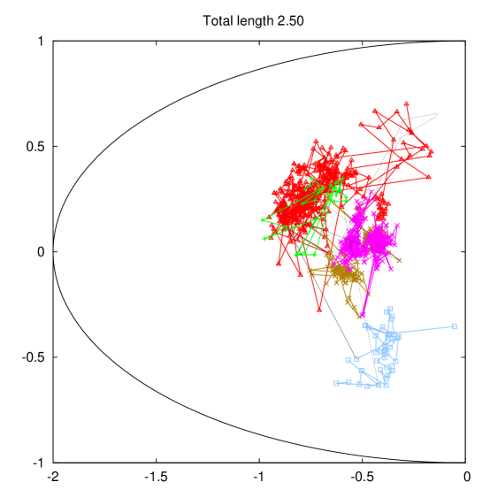
shows only the leftmost clump from Fig. 5, further split by the same algorithm with the threshold now $40^{\circ}$. The motion within the clump is not just random wandering. In fact the clump can be seen to be made up of 5 major sub-clumps with a certain degree of overlap. Such a structure is what one would expect in a scaling regime. If one separates clumps at a certain angular threshold, the size of the clumps as a fraction of the horizon size should not change with time. Thus clumps at later times should be composed of many clumps that existed at earlier times. These clumps are made smaller by damping due to the expansion of the universe. Thus at any given time, each large clump should consist of several smaller clumps separated by smaller angles, and so on.

Since our simulation begins with piecewise-linear initial conditions, one might worry that the clumping structure is related to the kinks that were present in the initial conditions. To investigate this possibility, in Fig. 7

Figure 7: Magnified view of the bottom clump of Fig. 5. Kinks that were present in the initial conditions are shown in blue (gray); those that were formed by later intersections are shown in black. The latter includes the kinks that go into and come out of the clump. The path of $\mathbf{a}^{\prime}$ sometimes jumps to a new value and then back again, leading to lines that appear to end.

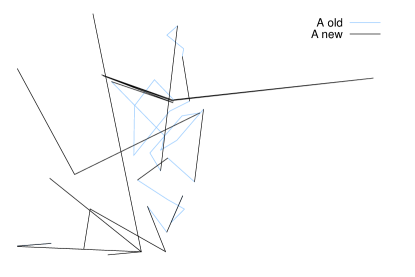
we distinguish the kinks that were present in the initial conditions from those occurred later at reconnections. While some of the structure comes from the initial conditions, a significant portion was added later.

Our picture of string shapes is thus the following. The tangent vector $\mathbf{a}^{\prime}$ on a long string wanders over small areas of the unit sphere to form small clumps, then jumps to another nearby area to form another small clump. Nearby small clumps form a single larger clump, and larger jumps connect the larger clumps, and so on. The path of $\mathbf{a}^{\prime}$ or $\mathbf{b}^{\prime}$ on a loop at formation is simply a section of the path that existed in a long string, with the ends of that section connected by one new kink formed when the loop was broken off, thus it has the same structure, and we do not expect cusps on newly-formed loops.

IV Gravitational smoothing

Now we turn to the effects of gravitational back reaction on the shape of strings. The general expectation, going back to the work of Quashnock and Spergel Quashnock and Spergel (1990) is that kinks formed at time $t_{1}$ will be smoothed out by a later time $t_{2}$ over length $\Gamma G\mu(t_{2}-t_{1})$, where $\Gamma\sim 50$. This effect limits the depth of the hierarchy of clumps and sub-clumps. Since the kinks in small sub-clumps were generally formed long ago, sub-clumps with $\sigma<\Gamma G\mu t$ do not exist at time $t$. Instead, at such scales the string is smooth.

On long strings, or recently formed loops, this effect is minimal. Observational constraints limit $G\mu$ to be less than $10^{-8}$ (E.g., see Ref. Blanco-Pillado et al. (2014)) so $\Gamma G\mu<10^{-6}$. Only a tiny percentage of the energy goes into loops with sizes smaller than or comparable to $10^{-6}t$, so in general the effects of smoothing are small.

On the other hand, for old loops, the effect is very different. For a loop which has lost half its initial energy to gravitational radiation, the length of the loop and the smoothing scale are equal. Such a loop will be quite smooth and will likely have cusps at scales similar to its length. As discussed in the Introduction, loops with a significant degree of evaporation are the most important cosmologically, so it is crucial to understand the effect of gravitational back reaction on loop shapes.

Unfortunately, we do not know the effect of gravitational back reaction in detail, so we must resort to a toy model to understand these phenomena. As a loop radiates gravitational waves, it must lose energy. We expect small structures to radiate their energy away more quickly than large ones, so that small structures are damped more quickly, resulting in a smoothing of the loop. Thus we will attempt to understand effects of gravitational back reaction by progressively smoothing our loops using convolution.

There is a simple model of gravitational back-reaction for wiggles on a straight string Hindmarsh (1990); Siemens and Olum (2001). If one takes small-amplitude sinusoidal wiggles traveling in one direction on the string and large wiggles (representing the underlying loop in this case) traveling in the other, and if the difference in wavelengths is not too large Siemens and Olum (2001) one finds that the small wiggles are damped approximately as an exponential with time constant proportional to wavelength. After a fixed time period, wiggles of different wavelengths would be damped exponentially with exponents inversely proportional their wavelengths.

Following this idea, we would like to Fourier decompose the tangent vectors $\mathbf{a}^{\prime}$ and $\mathbf{b}^{\prime}$ and damp each harmonic $n$ by some factor $e^{-wk}$, where $w$ is a constant and $k=2\pi n/L$ is the wave number. This corresponds to convolving $\mathbf{a}^{\prime}$ and $\mathbf{b}^{\prime}$ with a Lorentzian of width $w$, i.e., $w/(\pi(\sigma^{2}+w^{2}))$.

Unfortunately, there is a constraint on the magnitude of the tangent vectors, $|\mathbf{a}^{\prime}|=|\mathbf{b}^{\prime}|=1$. Smoothing any nontrivial function $\mathbf{a}^{\prime}$ or $\mathbf{b}^{\prime}$ will decrease its magnitude and violate this constraint. We tried simply renormalizing by setting $\mathbf{a}^{\prime}\to\mathbf{a}^{\prime}/|\mathbf{a}^{\prime}|$ after smoothing, but this works very poorly. The additional function $1/|\mathbf{a}^{\prime}|$ is in general not very smooth and multiplying by it undoes most of the desired damping of the high frequency modes.

After trying several techniques to address this problem, we arrived at the following solution. Instead of just convolving with a Lorentzian of width $w$ and then renormalizing, we convolve many times with much narrower Lorentzians, and renormalize after each one. We use as our Lorentzian width 1/20 of the spacing between the points used to describe the function $\mathbf{a}^{\prime}$ or $\mathbf{b}^{\prime}$. (It may seem bit strange to convolve with something narrower than the point spacing, but since a Lorentzian falls off slowly, the kernel is still quite wide.) Distributing the renormalization through the smoothing procedure yields much better results. The short modes are in fact damped by approximately the amount they would have been without renormalization.

We would like to consider loops which have lost some fraction $f$ of their initial energy to gravitational radiation. What does this corresponds to in terms of Lorentzian smoothing? We consider the amplitude of the $n=1$ mode as a proxy for the total length. This amplitude is multiplied in the smoothing procedure by $\exp(-2\pi c)$, where $c=w/L$ is the ratio of the Lorentzian width to the string length. Thus we say that smoothing with coefficient $c$ has removed a fraction

$$f=1-\exp(-2\pi c)\,,$$ (3)

of the initial loop length, and choose $c$ to achieve any desired fraction of evaporation.

We have studied loops taken from two simulations of size 500 in the matter era and two of size 1000 in the radiation era. In each case, we looked at all loops produced in the second half of the simulation with the ratio of loop size to horizon size at least 0.01. For each loop we repeatedly smooth the loop by convolution, evolve it for at least one oscillation to check whether smoothing has introduced self- intersections, smooth the loop again, and so on. In all there are 7 smoothing steps. The steps involve amounts of smoothing corresponding to a total loss since formation of the fractions 1/128, 1/64, 1/32, 1/16, 1/8, 1/4 and 1/2 of the original loop energy. Since repeated smoothing with coefficients $c_{1},c_{2},c_{3}\ldots$ corresponds to a single smoothing step with coefficient $c=c_{1}+c_{2}+c_{3}+\cdots$, we determine the actual smoothing coefficients by solving the equations

$$1-e^{2\pi c_{1}} = 1/128\,,$$ (4)

$$1-e^{2\pi(c_{1}+c_{2})} = 1/64\,,$$ (5)

$$1-e^{2\pi(c_{1}+c_{2}+c_{3})} = 1/32\,,$$ (6)

and so on to determine the coefficients $c_{1}$ through $c_{7}$.

To simplify the smoothing procedure, which requires repeated fast Fourier transforms, we work with numbers of frequencies and numbers of points that are powers of 2. We start with a function $\mathbf{a}^{\prime}$ (and similarly $\mathbf{b}^{\prime}$) that is piecewise constant with non-uniform pieces. We Fourier transform this function, keeping at step $i$ some number $N_{i}$ frequencies (half of which are negative frequencies whose whose amplitudes are just the complex conjugate of the positive-frequency amplitudes). We smooth in Fourier space by multiplying by an exponential representing the transform of a narrow Lorentzian. Then we transform back into $N_{i}$ uniformly spaced points, adjust the new tangent vectors to have uniform magnitude, Fourier transform back into $N_{i}$ frequencies, and so on, until we have achieved the desired degree of smoothing for the given step. We choose

$$N_{i}=(4096,4096,2048,1024,512,256,128)\,,$$ (7)

so that frequency $N_{i}/2$, the highest we keep at each step, would be reduced by the Lorentzian convolution by about $10^{-7}$.

The smoothing procedure described above is the best we have found, but we tried several other procedures (e.g., using a Gaussian instead of a Lorentzian) and the results are all qualitatively similar.

V Smoothing Results

V.1 Smoothing of loops and their tangent vectors

We show in Fig. 8

Figure 8: Snapshots for several steps of the smoothing procedure for a loop of length 17.9 at time 1000 in the radiation era.

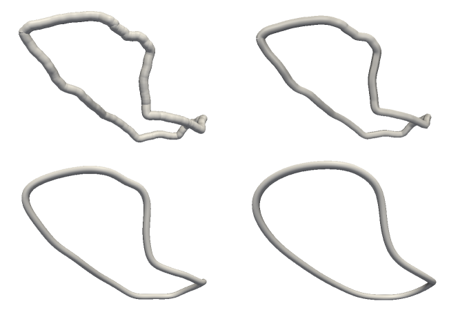
some pictures of a typical loop at different stages of the smoothing process. We see that indeed our smoothing procedure has removed small-scale structure from the loop.

In Fig. 9,

Figure 9: The effect of smoothing on the distribution of the $\mathbf{a}^{\prime}$ and $\mathbf{b}^{\prime}$ in the loop shown in Fig. 8. We see the production of a small loop from a region of high velocity where the ${\bf a^{\prime}\approx\bf b^{\prime}}$ after step 3 of our smoothing procedure. We mark the region of interest with a shaded disk near the center of the figure. The ejection of this loop is seen by the disappearance of a series of points of ${\bf a^{\prime}}$’s as well ${\bf b^{\prime}}$’s. Subsequent smoothing reconnects these points and smooths the string again.

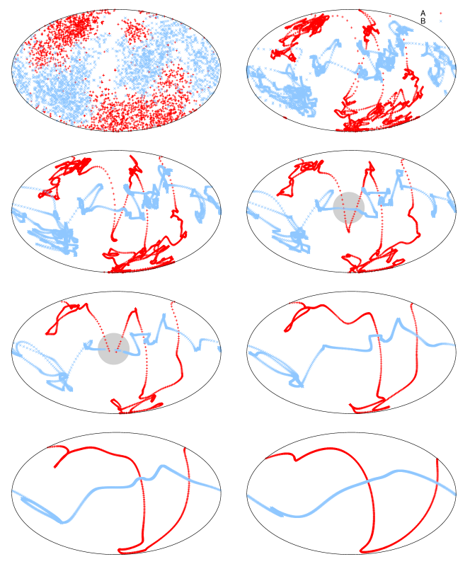
we show an example of the change in the paths of $\mathbf{a}^{\prime}$ and $\mathbf{b}^{\prime}$ on the Kibble-Turok sphere for a particular loop across the different stages of smoothing. We can clearly see that the procedure smooths out structures at increasingly large scales on the figure. A fragmentation event can be seen in these figures as a sharp disappearance of a collection of segments in both the ${\bf a^{\prime}}$’s and the ${\bf b^{\prime}}$’s. We have chosen a particular loop where we can see this clearly. After each fragmentation process, the remaining loop is not generally in the rest frame, so we boost it back to its rest frame before we further evolve it.

V.2 Weighting of simulation data

When we discuss the fraction of loops with certain properties, we are interested in the fraction of loops of any given size existing at some given time. What the simulation gives us, however, is a set of loops of different sizes produced in the same interval of time. As explained in Ref. Blanco-Pillado et al. (2014), each loop should thus enter into all histograms and averages with weight $x^{\delta}$, where $x$ is the ratio of the rest energy of the loop in units of $\mu$ to the horizon distance at the time of formation, and $\delta=1$ for matter and $3/2$ for radiation. All results below use this weighting procedure.

V.3 Fragmentation

The first question we ask is whether smoothing causes loops in non-self-intersecting trajectories to self-intersect and fragment. The answer is that this is not an important process. In our simulations, $90\%$ of the loops survive the smoothing procedure until half of their energy is eliminated by gravitational radiation with loss of no more than $10\%$ of their energy into fragmentation. We have followed this procedure for loops obtained in simulations in the radiation and matter era and we do not see significant variations on these numbers for the two cases.

Looking at movies of the loop evolution after fragmentation we have identified two major sources of loop fragmentation which are quite distinct and that pretty much cover all the cases where there is significant energy lost into loops by the parent loop.

Most of the cases where fragmentation occurs seem to be coming from fast-moving regions of the parent loop. The loops being produced from those regions are typically small but often have high Lorentz boosts. Furthermore there are several cases where we have seen trains of small loops created from those regions.

The other kind of fragmentation comes from the late time smoothing of the loop where the smoothing length is already comparable to the size of the loop. It is not clear how much one should trust this limiting regime of the smoothing process so in some sense we may be overestimating the amount of fragmentation by including these possible energy losses.

V.4 Number of Cusps

As shown in Fig. 9, the smoothing procedure yields an important reduction of the number of crossings between the $\mathbf{a}^{\prime}$ and the $\mathbf{b}^{\prime}$ functions on the sphere. We plot in Fig. 10 the distribution of the number of cusps for loops directly from the simulation, after two smoothing steps, and after the final step of the the smoothing procedure. We see that the number of “cusps” gets dramatically reduced already in the first stages of smoothing and quickly settles to 2 cusps per loop either for radiation or matter.

Figure 10: Distribution for the number of cusps before smoothing, after two smoothing steps, and when the loop is fully smoothed. Initially there are very many cusps, but these are really just crossings of kinks. By the end there are almost always 2 cusps in both cases.

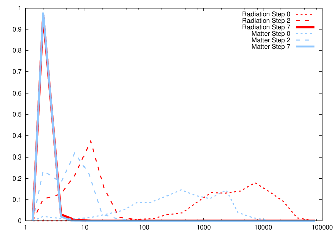
Furthermore, the amount of energy or length involved in each crossing increases from a very small amount to a considerable fraction of the total energy of the loop at the final stage of our smoothing procedure. In order to quantify this we estimate the value of the length associated with the second derivative of $\mathbf{a}$ and $\mathbf{b}$ at the point of the cusp by calculating

$$\alpha_{\text{c}usp}={{2\pi}\over{L|{\bf a^{\prime\prime}}_{\text{c}usp}|}}\,,$$ (8)

and similarly for $\beta_{\text{c}usp}$ in terms of $\mathbf{b}^{\prime\prime}$. We show in Fig. 11

Figure 11: Distribution of the value of the cusp parameter $\sqrt{\alpha\beta}$ at the same steps as in Fig. 10. Initially the “cusps” are infinitesimal, but by the end they involve most of the loop.

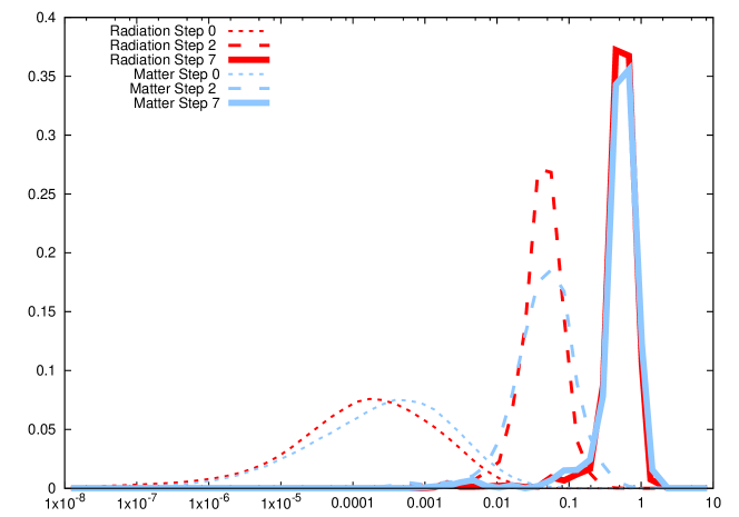
the distribution for the values of $\sqrt{\alpha\beta}$ at different stages of smoothing. We use the product $\alpha\beta$ because this is the area of the world sheet that is involved in the cusp, and controls, for example, the amount of gravitational radiation emitted Damour and Vilenkin (2001).

As we mentioned earlier, at the time of loop formation, there are a very large number of “cusps”, but these are really crossings of kinks that have no significant energy as can be seen in Fig. (11). On the other hand, nearly all smoothed loops have 2 cusps per oscillation, and these cusps are quite substantial.

V.5 Angular Momentum

The angular momentum of a loop is defined by the expression,

$${\bf J}=\mu\int_{0}^{L}{\left({\bf x}\times{\bf\dot{x}}\right)d\sigma}\,,$$ (9)

which can be written in terms of the the ${\bf a}$ and ${\bf b}$ functions by

$${\bf J}={{\mu}\over{4}}\int{\left({\bf a}\times\mathbf{a}^{\prime}+{\bf b}\times\mathbf{b}^{\prime}\right)d\sigma}\,.$$ (10)

It is useful to define a dimensionless quantity that compares the angular momentum of a loop of certain size $L$ to the maximum angular momentum for a loop of that energy,

$${\cal J}={{|{\bf J}|}\over{J_{max}}}=4\pi{{|{\bf J}|}\over{\mu L^{2}}}\,.$$ (11)

We show in Fig. 12 the weighted histogram of the angular momentum for the distribution of loops in our simulation. The initial distribution of loops as they come out of the simulation seem to have a somewhat larger typical angular momentum than the one found earlier in Scherrer et al. (1990). This is probably due to the statistical difference of the loops considered in these earlier studies compared with our scaling loops. We see that the distribution moves towards a larger fraction of the total possible angular momentum after smoothing has taken place. This does not mean, of course, that angular momentum increases but only that it grows relative to the total energy on the loop. One can understand this by realizing that most of the total angular momentum of the loop comes from the bulk motion of the loop and not the small scale structure on it. Smoothing reduces the small scale structure but does not have a great effect on the angular momentum. It would be interesting to see whether a more realistic model of back reaction changes this picture since gravitational waves should radiate part of the angular momentum on the loop.

Figure 12: Distribution of the angular momentum of the loops before and after smoothing.

V.6 Planarity

Copi and Vachaspati Copi and Vachaspati (2011) studied the degree to which cosmic string loops line in a plane. Their loops were formed by fragmentation of single loops with specified harmonics. Here we do a similar analysis of loops coming from our simulations and their smoothed versions. We consider the tensor

$${\cal I}_{ij}=\int dt\,d\sigma\,x_{i}(\sigma,t)x_{j}(\sigma,t)\,,$$ (12)

where the integral is taken over one oscillation and the coordinates are in the rest frame of the loop. This tensor (related to the quadrupole and moment of inertia tensors) gives the extent of the string world sheet in different directions. If the motion of the loop is confined to a plane, ${\cal I}$ will have a zero eigenvalue in the perpendicular direction. If the world sheet extends in all spatial directions equally, then the 3 eigenvalues of ${\cal I}$ will be equal. Thus we define the planarity,

$${\cal P}=1-\left({{\text{ minimum~{}eigenvalue of~{}}{\cal I}}\over{\text{average~{}eigenvalue of~{}}{\cal I}}}\right)\,,$$ (13)

which takes on values ranging from 0 for spherical symmetry to 1 for a planar loop.

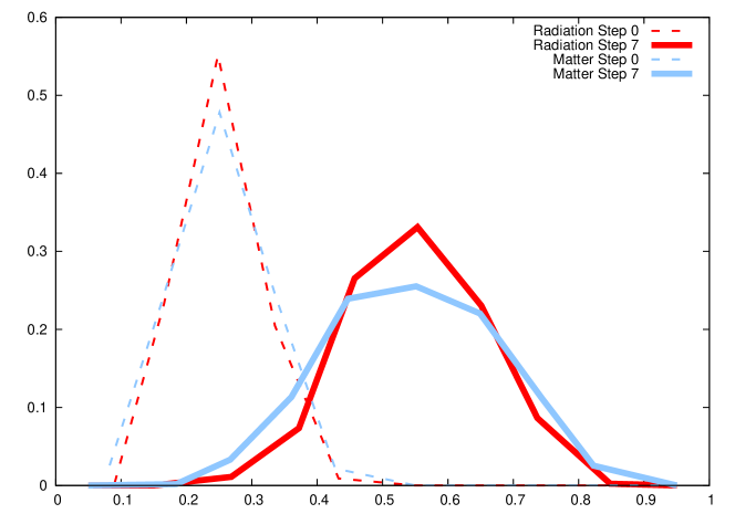
We can compute ${\cal I}$ by integrating over $\mathbf{a}$ and $\mathbf{b}$ separately. The results are shown in Fig. 13.

Figure 13: Distribution of the planarity measure ${\cal P}_{\cal I}$ for loops at formation and after the last smoothing step.

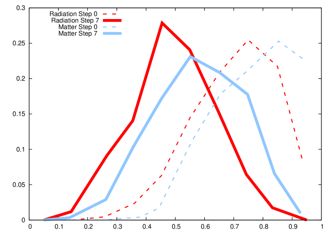
We find that loops at formation are significantly planar, ${\cal P}\sim 0.8$ or 0.9, but smoothing makes them more three-dimensional.

Ref. Copi and Vachaspati (2011) performed the same tensor calculation, but on $\mathbf{a}$ and $\mathbf{b}$ separately, rather than on $\mathbf{x}$. They found the two parts of the string to be substantially linear, with the largest eigenvalue of order 0.85 of the sum of the eigenvalues. Adding together the two mostly linear parts of the string yields a mostly planar shape, similar to what we found here for loops at formation. Ref. Copi and Vachaspati (2011) did not attempt to simulate gravitational smoothing.

VI Conclusions

We have analyzed the shape of loops and long strings in large cosmic string network simulations. Contrary to the usual view that strings are smooth, we find that long strings consist of generally straight segments punctuated by large-angle kinks. We find that the tangent vectors $\mathbf{a}^{\prime}$ and $\mathbf{b}^{\prime}$ to the right- and left-moving parts of strings form hierarchical “clumps” on the unit sphere. We do not see places where $\mathbf{a}^{\prime}$ and $\mathbf{b}^{\prime}$ trace out smooth paths.

When a loop forms, it inherits the $\mathbf{a}^{\prime}$ and $\mathbf{b}^{\prime}$ of the string from which it formed. Thus loops at formation do not have smooth regions of $\mathbf{a}^{\prime}$ and $\mathbf{b}^{\prime}$ that could cross to form a cusp. Furthermore, fragmentation of loops nearly completely divides the unit sphere into regions with only $\mathbf{a}^{\prime}$ and those with only $\mathbf{b}^{\prime}$. Only in unusual cases where these tangent vectors cross into each other’s regions could cusps be possible.

Nevertheless, gravitational back reaction will smooth loops and produce cusps on loops which formerly had only kinks. We study this process with a toy model and find that nearly all loops end up with 2 cusps per oscillation with most of the loop involved in the cusps.

The angular momentum of loops at the time of formation is about one quarter the maximum possible value, and increases by smoothing into about half the maximum possible value. This does not mean that the angular momentum of the loop is increasing, but rather that the length of the loop decreases during smoothing and that small-scale structure that does not contribute much to the overall angular momentum is the first to be eliminated.

At formation, loops have some degree of planarity, on the order of 0.85 as we described above. However, smoothing reduces the degree of planarity so that the smoothed loops are midway between a planar loop and a loop which has no preferred axes, with a wide distribution.

References

- Vilenkin and Shellard (2000) A. Vilenkin and E. P. S. Shellard, Cosmic Strings and other Topological Defects (Cambridge University Press, Cambridge, 2000).
- Zeldovich and Khlopov (1978) Y. B. Zeldovich and M. Yu. Khlopov, Phys. Lett. B79, 239 (1978).
- Preskill (1979) J. Preskill, Phys. Rev. Lett. 43, 1365 (1979).
- Kibble and Turok (1982) T. Kibble and N. Turok, Phys.Lett. B116, 141 (1982).
- Turok (1984) N. Turok, Nucl. Phys. B242, 520 (1984).
- Vachaspati (1987) T. Vachaspati, Gen. Rel. Grav. 19, 1053 (1987).
- Brandenberger (1987) R. H. Brandenberger, Nucl. Phys. B293, 812 (1987).
- Mohazzab (1994) M. Mohazzab, Int. J. Mod. Phys. D3, 493 (1994), arXiv:hep-ph/9307286 [hep-ph] .
- Blanco-Pillado and Olum (1999) J. J. Blanco-Pillado and K. D. Olum, Phys. Rev. D59, 063508 (1999), arXiv:gr-qc/9810005 [gr-qc] .
- Olum and Blanco-Pillado (1999) K. D. Olum and J. J. Blanco-Pillado, Phys. Rev. D60, 023503 (1999), arXiv:gr-qc/9812040 [gr-qc] .
- Vachaspati and Vilenkin (1985) T. Vachaspati and A. Vilenkin, Phys. Rev. D31, 3052 (1985).
- Damour and Vilenkin (2000) T. Damour and A. Vilenkin, Phys. Rev. Lett. 85, 3761 (2000), arXiv:gr-qc/0004075 [gr-qc] .
- Damour and Vilenkin (2001) T. Damour and A. Vilenkin, Phys. Rev. D64, 064008 (2001), arXiv:gr-qc/0104026 [gr-qc] .
- Vilenkin and Vachaspati (1987) A. Vilenkin and T. Vachaspati, Phys. Rev. Lett. 58, 1041 (1987).
- Spergel et al. (1987) D. N. Spergel, T. Piran, and J. Goodman, Nucl. Phys. B291, 847 (1987).
- Blanco-Pillado and Olum (2001) J. J. Blanco-Pillado and K. D. Olum, Nucl. Phys. B599, 435 (2001), arXiv:astro-ph/0008297 [astro-ph] .
- Cai et al. (2012) Y.-F. Cai, E. Sabancilar, and T. Vachaspati, Phys. Rev. D85, 023530 (2012), arXiv:1110.1631 [astro-ph.CO] .
- Srednicki and Theisen (1987) M. Srednicki and S. Theisen, Phys. Lett. B189, 397 (1987).
- Damour and Vilenkin (1997) T. Damour and A. Vilenkin, Phys. Rev. Lett. 78, 2288 (1997), arXiv:gr-qc/9610005 [gr-qc] .
- Peloso and Sorbo (2003) M. Peloso and L. Sorbo, Nucl. Phys. B649, 88 (2003), arXiv:hep-ph/0205063 [hep-ph] .
- Sabancilar (2010) E. Sabancilar, Phys. Rev. D81, 123502 (2010), arXiv:0910.5544 [hep-ph] .
- Long et al. (2014) A. J. Long, J. M. Hyde, and T. Vachaspati, JCAP 1409, 030 (2014), arXiv:1405.7679 [hep-ph] .
- Long and Vachaspati (2014) A. J. Long and T. Vachaspati, JCAP 1412, 040 (2014), arXiv:1409.6979 [hep-ph] .
- Burden (1985) C. J. Burden, Phys. Lett. B164, 277 (1985).
- Garfinkle and Vachaspati (1987) D. Garfinkle and T. Vachaspati, Phys. Rev. D36, 2229 (1987).
- Blanco-Pillado et al. (2014) J. J. Blanco-Pillado, K. D. Olum, and B. Shlaer, Phys. Rev. D89, 023512 (2014), arXiv:1309.6637 [astro-ph.CO] .
- Blanco-Pillado et al. (2011) J. J. Blanco-Pillado, K. D. Olum, and B. Shlaer, Phys. Rev. D83, 083514 (2011), arXiv:1101.5173 [astro-ph.CO] .
- Blanco-Pillado et al. (2012) J. J. Blanco-Pillado, K. D. Olum, and B. Shlaer, J. Comput. Phys. 231, 98 (2012), arXiv:1011.4046 [physics.comp-ph] .
- Scherrer et al. (1990) R. J. Scherrer, J. M. Quashnock, D. N. Spergel, and W. H. Press, Phys. Rev. D42, 1908 (1990).
- Copi and Vachaspati (2011) C. J. Copi and T. Vachaspati, Phys. Rev. D83, 023529 (2011), arXiv:1010.4030 [hep-th] .
- Quashnock and Spergel (1990) J. M. Quashnock and D. N. Spergel, Phys. Rev. D42, 2505 (1990).
- Hindmarsh (1990) M. Hindmarsh, Phys. Lett. B251, 28 (1990).
- Siemens and Olum (2001) X. Siemens and K. D. Olum, Nucl. Phys. B611, 125 (2001), arXiv:gr-qc/0104085 [gr-qc] .
- Green et al. (1988) M. B. Green, J. H. Schwarz, and E. Witten, Superstring Theory. Vol. 1: Introduction (Cambridge University Press, Cambridge, 1988).