Haloes light and dark: dynamical models of the stellar halo and constraints on the mass of the Galaxy

Abstract

We develop a flexible set of action-based distribution functions (DFs) for stellar haloes. The DFs have five free parameters, controlling the inner and outer density slope, break radius, flattening and anisotropy respectively. The DFs generate flattened stellar haloes with a rapidly varying logarithmic slope in density, as well as a spherically aligned velocity ellipsoid with a long axis that points towards the Galactic centre – all attributes possessed by the stellar halo of the Milky Way. We use our action–based distribution function to model the blue horizontal branch stars extracted from the Sloan Digital Sky Survey as stellar halo tracers in a spherical Galactic potential. As the selection function is hard to model, we fix the density law from earlier studies and solve for the anisotropy and gravitational potential parameters. Our best fit model has a velocity anisotropy that becomes more radially anisotropic on moving outwards. It changes from $\beta\approx 0.4$ at Galactocentric radius of 15 kpc to $\approx 0.7$ at 60 kpc. This is a gentler increase than is typically found in simulations of stellar haloes built from the mutiple accretion of smaller systems. We find the potential corresponds to an almost flat rotation curve with amplitude of $\approx 200$ kms^-1 at these distances. This implies an enclosed mass of $\approx 4.5\times 10^{11}M_{\odot}$ within a spherical shell of radius $50{\,\mathrm{kpc}}$.

1 INTRODUCTION

It has long been known that the distribution functions (DFs) of collisionless stellar systems depend on the integrals of motion. This result is often called Jeans (1919) Theorem, though it was known earlier to Poincaré. A number of choices of integrals of motion are possible. These include the classical integrals such as energy or angular momentum (e.g., Eddington, 1915; Hunter & Qian, 1993; Evans & An, 2006), the turning points or apocentric and pericentric distances of orbits (Hunter & de Zeeuw, 1992), or the actions (e.g., Binney & Spergel, 1984; Binney, 1987). Although there are advantages and disadvantages to any of these choices, the actions remain very appealing because they are adiabatically invariant and they form a canonical set of coordinates when combined with the conjugate angles (see e.g., Goldstein, 1980).

Historically, actions have not been much used in stellar dynamics because of the difficulty in calculating them. For classical problems like the Keplerian potential or the harmonic oscillator, they can be readily evaluated by residue calculus (Born, 1927). The isochrone is the most general spherical potential for which the actions are available as elementary functions (e.g., Henon, 1959; Evans et al., 1990). For the separable or Stäckel potentials, they are available as a quadrature and provide a beautiful demarcation of phase space in terms of the orbital types (de Zeeuw, 1985). However, the last few years have seen a major change, in that a number of methods have been proposed to enable the rapid evaluation of actions in a variety of potentials. This includes the adiabatic approximation (Binney, 2010), local fitting (Sanders, 2012) and the Stäckel fudge (Binney, 2012a; Sanders & Binney, 2015a). Together with the release of software packages like galpy (Bovy, 2015), this work has transformed the calculation of actions into a routine matter for most axisymmetric and triaxial potentials.

The form of the DF in action space is now an interesting problem to study. The complex nature of galaxies suggests that each component – bulge, disk, stellar halo and dark halo — needs its own distribution function and is described by a characteristic shape in action space (Binney, 1987). The functional form of the DF for thin and thick stellar disks is suggested by warming up models based on pure circular or epicyclic orbits and has been studied extensively in recent years, motivated by applications to the Milky Way (see e.g., Binney, 2010; Bovy & Rix, 2013). Binney (2012b) showed that action-based DFs fit to the Geneva-Copenhagen Survey of nearby stars (Nordström et al., 2004) accurately predict the kinematics of stars in the deeper Radial velocity experiment (RAVE, Steinmetz et al., 2006). Subsequently, Sanders & Binney (2015b) introduced extended DFs for the Galactic disk by introducing an analytic dedendence on metallicity. However, hot components such as bulges, dark matter haloes and stellar haloes have received much less attention. Posti et al. (2015) and Williams & Evans (2015) considered self–consistent models with double power-law density profiles. In principle, such DFs can be used for stellar and dark haloes, as well as elliptical and dwarf spheroidal galaxies. However, these papers did not provide any fits to large datasets. We aim to remedy this deficiency here, by using such models to represent the Milky Way’s stellar halo as a tracer population in the Galactic potential.

Section 2 introduces our family of DFs which depend on the actions. These are motivated by the density law of the stellar halo, which is of a flattened double power-law form to a reasonable approximation. Section 3 provides a brief description of the data on blue horizontal branch stars extracted by Xue et al. (2011) from the Sloan Digital Sky Survey. As the selection function of the sample is unknowable, Section 4 outlines our fitting methodology. Section 5 presents our results, together with a comparison with other recent work on the Milky Way stellar halo. We sum up in Section 6, and suggest further extensions and applications of our models.

2 The dynamical model

In this section, we describe the construction of our dynamical model. First, we summarise the observational constraints already placed on the properties of the distribution function. We then demonstrate how these constraints can be used to construct a suitable model.

2.1 Observational motivation

The spatial properties of the stellar halo are reasonably well-studied. Deason et al. (2011b) found that a sample of $\sim 20000$ Blue Horizontal Branch (BHB) and Blue Straggler (BS) stars taken from the Sloan Digital Sky Survey (SDSS) is well modelled by a flattened broken power law

$$\rho(\boldsymbol{r})\propto\begin{cases}\left(\dfrac{r_{q}}{{r_{\mathrm{b}}}}\right)^{-{\alpha_{\mathrm{in}}}}&r_{q}<{r_{\mathrm{b}}},\\ \\ \left(\dfrac{r_{q}}{{r_{\mathrm{b}}}}\right)^{-{\alpha_{\mathrm{out}}}}&r_{q}>{r_{\mathrm{b}}},\end{cases}$$ (1)

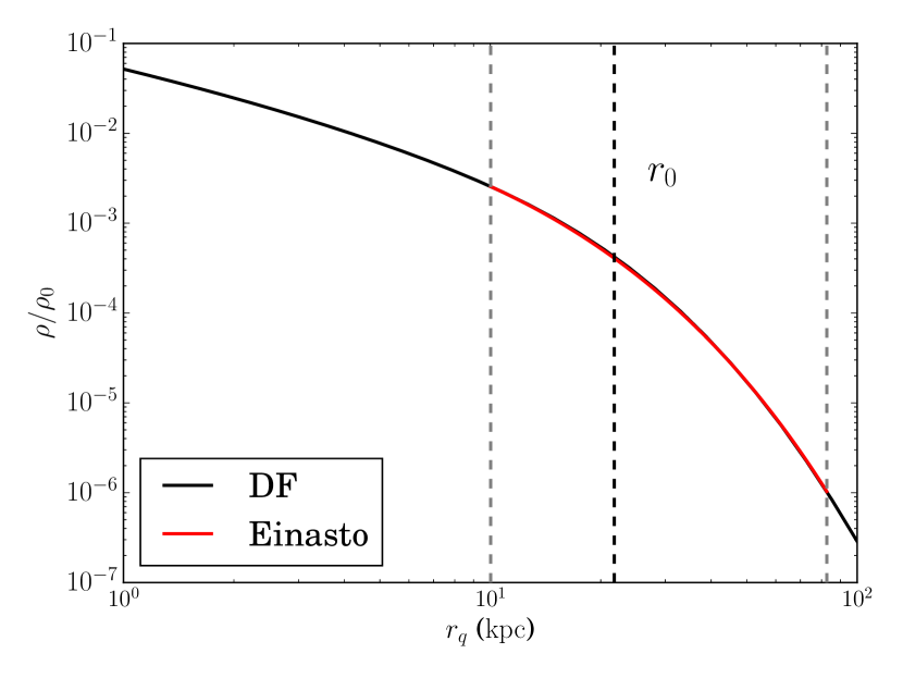
where $r_{q}^{2}=R^{2}+(z/q)^{2}$. Their best-fit parameters are ${r_{\mathrm{b}}}=27{\,\mathrm{kpc}}$, ${\alpha_{\mathrm{in}}}=2.3$, ${\alpha_{\mathrm{out}}}=4.6$ and $q=0.59$. Other studies have provided similar, though not identical, results (see e.g., Pila-Díez et al., 2015) and so we can be confident that the stellar-halo density is well-represented by oblate models with a sharp change in gradient in the density profile at $\sim 30{\,\mathrm{kpc}}$. This rapidly changing gradient in the density is equally well described by the Einasto density law

$$\rho(r_{q})\propto\exp\left(-d_{n}\left[\left(r_{q}/r_{\mathrm{eff}}\right)^{1/n}-1\right]\right),$$ (2)

where $d_{n}=3n-1/3+0.0079/n$. Deason et al. (2011b) also fit such a profile in their analysis, with best fit parameters are $\left(n,q,r_{\mathrm{eff}}\right)=\left(1.7,0.58,20{\,\mathrm{kpc}}\right)$.

The structure of halo stars in velocity space is not as well constrained, which is primarily explained by the comparative lack of information: we possess all three spatial coordinates, but usually only one component of the velocity (the line–of–sight velocity), of each halo star. Nonetheless, the fact that the sun resides at a distance from the Galactic Centre still allows us to place constraints on the velocity ellipsoid of the stellar halo. Bond et al. (2010) used a large sample of SDSS halo stars to investigate the velocity structure within $r_{\mathrm{GC}}\sim 10{\,\mathrm{kpc}}$, and found that the velocity ellipsoid is essentially spatially invariant within their distance limit. Their inferred ellipsoid aligns with spherical coordinates, with axes given by $\sigma_{r}=141{\,\mathrm{kms^{-1}}}$, $\sigma_{\phi}=85{\,\mathrm{kms^{-1}}}$ and $\sigma_{\theta}=75{\,\mathrm{kms^{-1}}}$. The spherical anisotropy parameter, given by

$$\beta(r)=1-\dfrac{\sigma_{\phi}^{2}+\sigma_{\theta}^{2}}{2\sigma_{r}^{2}},$$ (3)

has a value of $\sim 0.65$. Other studies of halo kinematics find similar results, with $\beta$ usually between 0.4 and 0.6 (e.g., Smith et al., 2009).

Figure 1: Distributions of stars in the BHB dataset. Top: Histogram of Galactocentric distance. Middle: Distribution of Galactocentric distance and line–of–sight velocity. Note there is a noticeable overdensity at $r\sim 35{\,\mathrm{kpc}}$ due to Sagittarius stream members. Bottom: Positions on the sky of the BHB sample after our cuts have been made. The dashed horizontal lines are at $|b|=30\degree$, which define our cut in Galactic latitude in order to avoid disc stars.

2.2 Distribution function and gravitational potential

Given the observational constraints, we wish to construct a DF that generates a flattened density profile with a rapidly changing logarithmic slope, and with a velocity ellipsoid that is is spherically aligned and radially biased. Our model consists of a DF for the BHB population and a parameterisation of the Galactic gravitational potential. We choose to model the potential in a very simple way, using a spherical power law

$$\Phi(r)=-\dfrac{v_{0}^{2}}{\delta}\left(\dfrac{r}{10\,{\,\mathrm{kpc}}}\right)^{-\delta},$$ (4)

where $0<\delta<1$. Although the true Galactic potential is significantly more complex, this simple approximation is motivated by recent studies of the Galactic potential far from the disk. For example, in a recent study of the GD1 stream, Bowden et al. (2015) found the potential to be well described by a scale–free and modestly flattened ($q=0.91\pm 0.04$) model at distances $r_{\mathrm{GC}}\sim 15{\,\mathrm{kpc}}$. Using the same stream generation method, Gibbons et al. (2014) showed that the mass profiles of flattened model galaxies are nonetheless accurately recovered using a model potential that is spherical. Furthermore, the spherical alignment of the velocity ellipsoid is also suggestive that the gravitational potential is itself close to spherically symmetric at large radii (Evans et al. 2015). That said, our over–simplification of the Galactic potential is only permissible in a first attempt to fit data with action-based DFs, and should be superseded in later work. In particular, evidence on the shape of the dark matter halo of the Galaxy is confused, and trivial as well as axisymmetric shapes remain possible (e.g., Law et al., 2009; Law & Majewski, 2010; Vera-Ciro & Helmi, 2013; Deg & Widrow, 2013).

In a spherical potential, the actions are the azimuthal action $J_{\phi}$, which is equal to the angular momentum about the $z$-axis; the latitudinal action $J_{\theta}=L-|J_{\phi}|$, where $L$ is the specific angular momentum, and the radial action

$$J_{r}=\dfrac{1}{2{\mathrm{\pi}}}\int\sqrt{2\left[E-\Phi(r)\right]-L^{2}/r^{2}}{\mathrm{d}}r.$$ (5)

Since our choice of gravitational potential is a power-law, the result found by Williams et al. (2014) applies, which gives the Hamiltonian of a generic power law as a function of the actions

$$H({\boldsymbol{J}})=C\left(L+DJ_{r}\right)^{\zeta}=C\mathcal{L}^{\zeta},$$ (6)

where $C$, $D$ and $\zeta$ are functions of the power law index $\delta$ (for full expressions see Williams et al. 2014). Williams & Evans (2015) then showed that a model with two power–law regimes is generated by a DF of the form

$$f({\boldsymbol{J}})\propto\dfrac{\mathcal{L}^{-\lambda}}{\left(\mathcal{L}^{2}+{J_{\mathrm{b}}}^{2}\right)^{(\mu-\lambda)/2}},$$ (7)

where ${J_{\mathrm{b}}}$ is the ‘break action’, and controls the location of the break in the density profile of the model. We expect our DF to broadly resemble this ansatz, although here we are modelling a tracer population in an independent potential rather than building a self–consistent model. The DF of Equation (7) generates a spherically symmetric, isotropic double power-law model in the potential of Equation (4), since $\mathcal{L}$ is very nearly a function of energy alone. The parameters $\mu$ and $\nu$ are related to the logarithmic slopes of the stellar halo density profile ${\alpha_{0}}$ and ${\alpha_{\infty}}$ by

$$\lambda=\zeta\left({\alpha_{0}}/\delta-3/2\right),$$

$$\mu=\zeta\left({\alpha_{\infty}}/\delta-3/2\right).$$ (8)

In order to give the model an anisotropic, spherically aligned velocity ellipsoid, we follow Williams & Evans (2015), who demonstrated that modifying the argument $\mathcal{L}$ to the DF such that

$$\mathcal{L}\rightarrow L+fDJ_{r},$$ (9)

($f>0$) endows the model with anisotropic kinematics. This arises because the factor $f$ alters the relative importance of high and low eccentricity orbits. If $0<f<1$, then the model becomes radially biased, and $f>1$ gives tangentially biased models.

Our final modifications to the DF will have the effect of breaking the spherical symmetry of the model density profile, so that it becomes flattened. In action space, this means introducing an explicit dependence on $J_{\phi}$, which will give the model a symmetry axis. de Bruijne et al. (1996) discovered a very elegant method for this purpose, though only for scale–free models. Remarkably, they found that introducing a multiplicative factor has precisely this effect. This factor is given by

$$h(e^{2}J_{\phi}^{2}/L^{2})=\sum\limits_{k=0}^{\infty}\dfrac{(1)_{k}(\frac{\alpha}{2})_{k}}{k!(\frac{1}{2})_{k}}\left(\dfrac{e^{2}J_{\phi}^{2}}{L^{2}}\right)^{k},$$ (10)

where $e=\sqrt{1-q^{2}}$ is the ellipticity, $(...)_{k}$ is the Pochammer symbol and $\alpha$ is the power law slope in the density. This factor has the effect of reducing the number of stars on orbits where the ratio $J_{\phi}/(|J_{\phi}|+J_{\theta})$ is small, which reduces the amount of vertical motion in the model relative to the circulation around the symmetry axis, thereby flattening the density profile. The expression at first sight appears unwieldy due to the sum to infinity, but numerical experiments demonstrate that the series converges very quickly, after $\sim 10$ terms. As it stands, this expression is inappropriate for our purposes, since it is designed for scale–free densities. We make the replacement

$$\alpha\rightarrow\alpha({\boldsymbol{J}})=\dfrac{{\alpha_{0}}+{\alpha_{\infty}}(|{\boldsymbol{J}}|/{J_{\mathrm{b}}})^{2}}{1+(|{\boldsymbol{J}}|/{J_{\mathrm{b}}})^{2}},$$ (11)

where $|{\boldsymbol{J}}|=\sqrt{\sum\nolimits J_{i}^{2}}$. This approximately preserves the constant flattening of the model. A suitable DF is therefore

$$f({\boldsymbol{J}})=\dfrac{\mathcal{N}}{{J_{\mathrm{b}}}^{3-\mu}(2{\mathrm{\pi}})^{3}}\dfrac{h({\boldsymbol{J}})\,\mathcal{L}^{-\lambda}}{\left(\mathcal{L}^{2}+{J_{\mathrm{b}}}^{2}\right)^{(\mu-\lambda)/2}},$$ (12)

where $\mathcal{N}$ is a normalisation factor such that

$$(2{\mathrm{\pi}})^{3}\int\,f({\boldsymbol{J}})\,{\mathrm{d}}^{3}{\boldsymbol{J}}=1,$$ (13)

and $h({\boldsymbol{J}})$ is given by Equations (10) and (11). We have now constructed a model with all of the desired properties motivated by observations. All of our parameters are nicely physical, except for the break action. In practise, we should like to replace this parameter with a break radius, ${r_{\mathrm{b}}}$. Unfortunately, a wholly analytical expression for ${J_{\mathrm{b}}}$ in terms of a break radius is unavailable. We can approximate ${J_{\mathrm{b}}}$ with the expression

$$\dfrac{{J_{\mathrm{b}}}}{1000{\,\mathrm{kms^{-1}}}{\,\mathrm{kpc}}}=\left(\dfrac{v_{0}}{100{\,\mathrm{kms^{-1}}}}\right)\,\dfrac{\delta^{1/\delta}}{\sqrt{\delta}}\,\left[\zeta-\frac{\zeta}{2}\delta(1-\mathrm{e}^{-1})\right]^{1/\zeta}\,\left(\dfrac{r_{0}}{10{\,\mathrm{kpc}}}\right)^{-\delta/\zeta}.$$ (14)

This expression is derived by considering the relative contributions of perfectly radial and circular orbits to the density profile of the model. For a given $r_{0}$ and $v_{0}$, the model density profile will break at an elliptical radius ${r_{\mathrm{b}}}\simeq r_{0}$ if ${J_{\mathrm{b}}}$ from the above expression is used as the break action. We then choose to sample the parameter $r_{0}$. The model parameters are then

$$\mathcal{P}=\left({\alpha_{0}},\,{\alpha_{\infty}},\,r_{0},\,q,\,f,\,v_{0},\,\delta\right),$$ (15)

each of which has a simple physical interpretation.

Figure 2: Likelihood contours from our analysis. We show the 68% and 95% confidence intervals of the marginalised distribution over pairs of model parameters, and mark the maximum likelihood gridpoint with a red cross. In the one–dimensional distributions, the maximum likelihood value for each parameter is marked with a dashed vertical line. One can see that the circular velocity at $10{\,\mathrm{kpc}}$ is tightly constrained, and that models close to logarithmic potentials are favoured. The contours of marginalised distributions involving $\delta$ are one–sided due to the fact that we only consider declining rotation curves. Our grid in $\delta$ was truncted at $\delta=10^{-2}$ because of the highly singular limit that occurs at $\delta=0$.

Figure 3: Spatial properties of the model. Left: the density profile of the model in the $x$–$z$ plane. Right: the 1D density profile of the model with elliptical radius. The black dashed line denotes the value of the parameter $r_{0}$, and the grey lines surround the region for which we have data. Overplotted in the range where the data lies is the best–fit Einasto profile from Deason et al. (2011b), which we use to constrain the density profile of our model.

3 Data

Figure 4: Comparisons of our maximum–likelihood model to the data. Top panel: the line–of–sight velocity dispersions of the data and mock catalogue as a function of Galactocentric radius. The two profiles are in excellent agreement, other than an upturn in the profile of the data at large radii. Middle: residuals between the model and the data in the dsitribution of Galactocentric radius and line–of–sight velocity. The residuals are essentially noise other than a feature between 30 and $50{\,\mathrm{kpc}}$ at $\sim-100{\,\mathrm{kms^{-1}}}$, which is due to stars belonging to the leading arm of the Sagittarius stream. Bottom: comparison of the distributions in line–of–sight velocity between the model and the data. The two distributions are in good agreement, except the data displays a slight skew towards negative line–of–sight velocities, due to the overdensity of Sagittatius stars at ${v_{\mathrm{LOS}}}\sim-100{\,\mathrm{kms^{-1}}}$.

In this study, we fit our model to the dataset provided by Xue et al. (2011), who compiled a catalogue of BHB stars from the SDSS DR8 catalogue (Aihara et al., 2011). The dataset contains $\sim 4000$ spectroscopically confirmed BHB candidates, arising from various spectroscopic surveys within SDSS. BHB stars are a very useful class of object to use when investigating the stellar halo, as they are intrinsically bright, with $M_{g}\sim 0.5$, and Deason et al. (2011b) showed that very accurate estimates of their absolute magnitudes can be derived ($\Delta M_{g}\sim 0.15$) via the polynomial relation

$$M_{g} = 0.434-0.169(g-r)+2.319(g-r)^{2}$$ (16)

$$+ 20.449(g-r)^{3}+94.517(g-r)^{4},$$

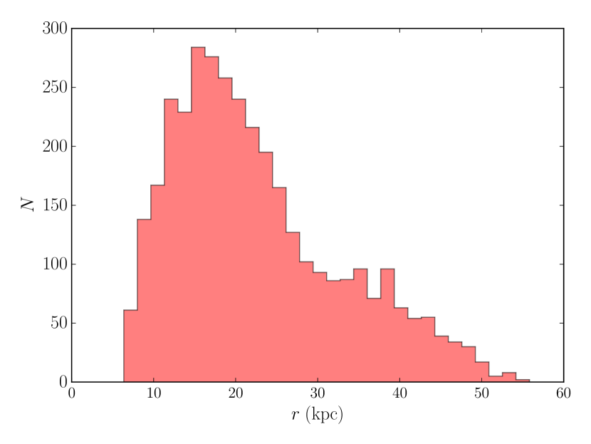
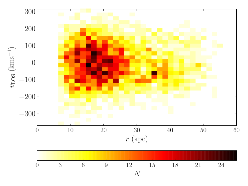
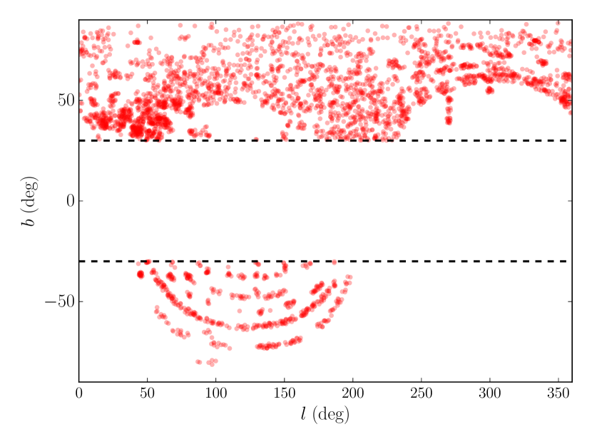
which is valid in the colour range $-0.25<g-r<0.0$. From the absolute magnitude, we can estimate distances to the stars in our sample to high precision. Before carrying out our analysis, we make two cuts on the dataset. First, we limit the colours to the range for which Equation (16) is valid, to ensure that the inferred distances are reliable. We then only include stars for which $|b|>30^{\circ}$ in order to reduce contamination from the disk. This leaves us with 3534 stars at Galactocentric radii $10{\,\mathrm{kpc}}\lesssim r\lesssim 50{\,\mathrm{kpc}}$, each of which has 4 of 6 phase–space coordinates very accurately constrained. Figure 1 depicts the distributions in Galactocentric distance, line–of–sight velocity and on–sky positions of the data.

4 Fitting Methodology

Ideally, we would like to use this dataset to constrain all the parameters of our model. This would mean inferring properties of the entire phase–space distribution of the stellar halo, including the density profile and kinematics. However, in order to carry out such a study, we would require detailed knowledge of the selection function of the sample of stars that is being used. The observed distribution of stars in phase–space and chemistry, $\boldsymbol{Z}$, is the product of the selection function with the true density, i.e.

$$f_{\mathrm{obs}}\left(\boldsymbol{x},\,\boldsymbol{v},\boldsymbol{Z}\right)=S\left(m\,,\,l\,,\,b\,,\,\boldsymbol{Z}\right)\times f_{\mathrm{true}}\left(\boldsymbol{x},\,\boldsymbol{v},\boldsymbol{Z}\right).$$ (17)

Note that the selection function, $S$, is presumed not to depend on the velocities of the stars, but does depend on their magnitudes ($m$), on–sky positions and chemistry. Without an effective model of $S$, we cannot hope to constrain the spatial and chemical distributions of the stars. Unfortunately, the selection function for our data is essentially unknown. Since the stars were observed on a variety of different plates from different spectroscopic surveys, and they have a relatively low on–sky density, we concluded that a reverse–engineered selection function of the sort used by Bovy et al. (2012) cannot be produced. This means inference on the density profile of the stellar halo is not possible with the data used here.

All hope is not lost, however. Although some of the parameters of our model cannot be constrained by this data, we can still proceed. We can use the independent analysis of Deason et al. (2011b) to place strong priors on the spatial distribution of the stars, and then proceed to use the velocities of the stars to constrain the kinematics of the stellar halo, as well as the Galactic mass profile. This is precisely what was done by Deason et al. (2012, hereafter D12), though they used a smaller subsample of $\sim 1900$ stars from this dataset. Our DF lets us model the entire dataset, and thus place tighter constraints on halo kinematics and the mass of the Galaxy, though of course the properties of the stellar halo such as the flattening ($q=0.59$) are fixed at outset.

Given the above discussion, we use the data to constrain only 3 of the 7 model parameters: $f$, which controls the kinematics, $v_{0}$, the circular speed at $10{\,\mathrm{kpc}}$, and $\delta$, the slope of the gravitational potential. The remaining parameters are fixed for each set of $(f\,,\,v_{0}\,,\,\delta)$ by optimizing the fit of our model’s density profile to the Einasto model of Deason et al. (2011b) described in Section 2.1. This stage of the procedure is equivalent to enforcing a very strong prior on the remaining 4 parameters of the model. The likelihood for an individual datum is then given by

$$p(v_{\mathrm{LOS,\,i}}\,|\,\boldsymbol{x}_{i}\,,\,f\,,\,v_{0}\,,\,\delta) = \int f({\boldsymbol{J}})\left|\dfrac{\partial({\boldsymbol{J}}\,,\,\boldsymbol{\theta})}{\partial(\boldsymbol{X})}\right|\,{\mathrm{d}}v_{l}\,{\mathrm{d}}v_{b}$$ (18)

$$/ \int f({\boldsymbol{J}})\left|\dfrac{\partial({\boldsymbol{J}}\,,\,\boldsymbol{\theta})}{\partial(\boldsymbol{X})}\right|\,{\mathrm{d}}v_{l}\,{\mathrm{d}}v_{b}{\mathrm{d}}v_{\mathrm{LOS}},$$

where $\boldsymbol{X}$ are the usual Galactic coordinates. The above expression simplifies, owing to the fact that the Jacobian factors depend only on position coordinates, giving

$$p(v_{\mathrm{LOS,\,i}}\,|\,\boldsymbol{x}_{i}\,,\,f\,,\,v_{0}\,,\,\delta)=\dfrac{1}{\rho(\boldsymbol{x}_{i})}\,\int f({\boldsymbol{J}})\,{\mathrm{d}}v_{l}\,{\mathrm{d}}v_{b},$$ (19)

which is the normalised line–of–sight velocity distribution at the position of the star in question. The log–likelihood for the entire dataset is then simply

$$\log l=\sum\limits_{j=1}^{N_{\mathrm{BHB}}}\log p_{j}.$$ (20)

In order to compute this likelihood with minimal noise, high–precision numerics are required for a number of different tasks. First, we need to evaluate the non–classical integral $J_{r}$ in order to compute the integrand $f({\boldsymbol{J}})$. In order to do this, we compute $J_{r}$ numerically using adaptive Gaussian quadrature implemented in the Gnu scientific library over a grid of 200 points in angular momentum at some fiducial energy $E_{0}$. Since the potential is scale–free, the radial action scales self–similarly with energy, so we do not need to consider other energies: $J_{r}$ can be recovered by simple multiplication by a scale factor. In–between grid points, we recover $J_{r}$ using cubic spline interpolation.

Once the radial action is available, we must perform the two (marginalising over the proper motions) and three–dimensional (integrating over velocities to find the density) integrals required to compute the normalised line–of–sight velocity distributions. This is done using the Cuhre algorithm implemented in the Cuba package (Hahn, 2005). This particular algorithm is deterministic, which guarantees that our likelihoods are replicable.

Evaluating the triple integral needed to calculate the density of the model at a given position is significantly more time-consuming than the double integral when marginalising over the proper motions. However, the model has a smooth two–dimensional density profile, and we can use this to our advantage. Instead of explicitly evaluating the density at the positions of all 3534 stars, we instead construct a grid and use bilinear interpolation to recover the density. An astute choice of variables proves to be

$$u = \frac{1}{2}\log\left(R^{2}+(z/q)^{2}\right),$$ (21)

$$t = \arctan\left(\dfrac{qR}{|z|}\right).$$

An economically sized grid can be used for interpolation to find the density. We use a grid of 20 points in $u$ and 10 points in $t$, and find that the density at the position of any star is recovered to a precision of 0.4 percent at worst.

All of the above calculations are performed in C, which is then wrapped for use in python. In order to locate the maximum–likelihood solution, we perform a grid–search. Monte–Carlo methods are unnecessary in this instance, due to the low dimensionality of the parameter space.

5 Results & Discussion

${\alpha_{0}}$	${\alpha_{\infty}}$	$r_{0}$	$q$	$f$	$v_{0}$	$\delta$
$0.84^{+0.07}_{-0.30}$	$9.13^{+0.96}_{-0.19}$	$21.6^{+1.5}_{-1.5}{\,\mathrm{kpc}}$	0.59	$0.59^{+0.07}_{-0.04}$	$198.2^{+3.4}_{-3.2}{\,\mathrm{kms^{-1}}}$	$0.01^{+0.006}_{-0.01}$

Table 1: Parameters of our maximum likelihood model and their dispersions. We do not quote a dispersion for the flattening, $q$, because it is kept fixed during the fitting procedure.

Here, we present the results of our analysis. First, we consider how well the model fits the data. Then we discuss the constraints placed on the Milky Way mass distribution and circular velocity profile, comparing our results with those from other analyses. finally, we discuss the kinematics of our best–fit model.

5.1 Comparison to the data

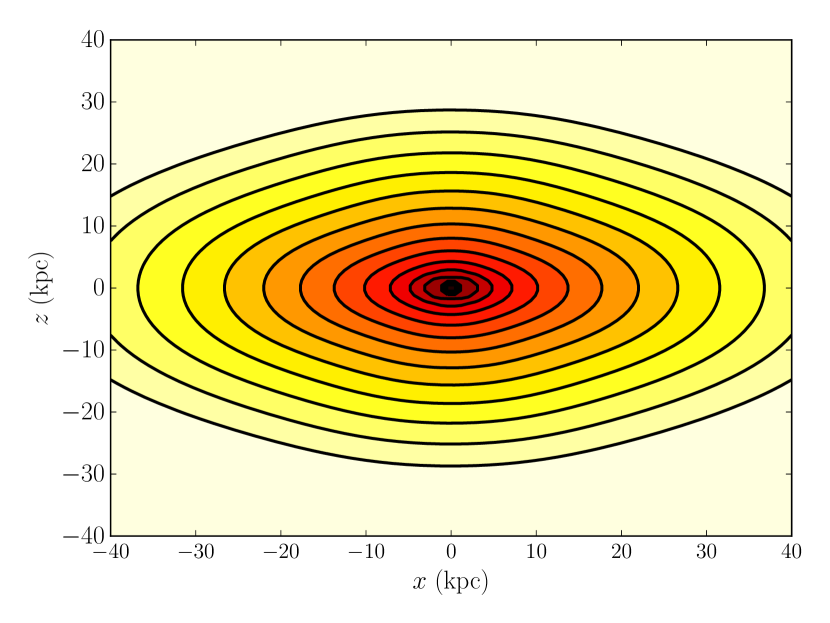
Figure 2 depicts the likelihood distributions from our analysis, and Table 1 summarises the best–fit parameters and their errors. Note that four of the parameters are fixed by our prior on the density profile, and Figure 3 depicts the one and two–dimensional properties of the density of this model.

In order to compare the model to the data, we generated a mock catalogue by drawing a line–of–sight velocity at the position in the Galaxy of each star from the maximum likelihood model. The reason we do not also sample position is because, as previously stated, the selection function is unknown and depends on the location of the star. We have assumed that the selection function does not depend on the kinematics of a star, and we are therefore safe to freely sample the line–of–sight velocity distributions of the model at positions where stars have been observed. We draw the mock catalogue using a simple rejection sampling technique.

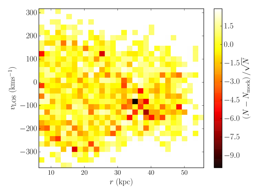
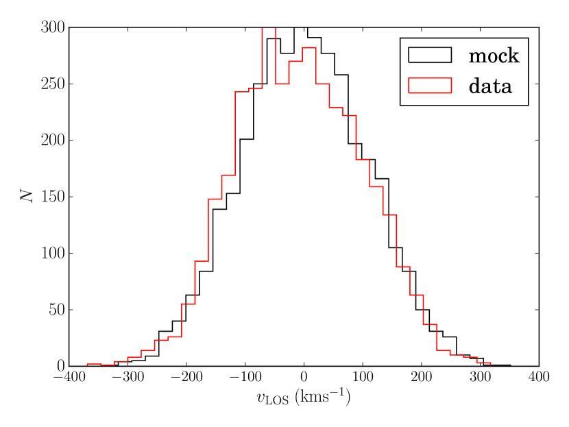
Figure 4 depicts several comparisons between the data and our mock catalogue. The upper panel, depicting the line–of–sight velocity dispersions as a function of galactocentric radius, shows excellent agreement between our model and the data. There is an upturn in the profile of the data at large radii, which is due to the presence of stars belonging to the Sagittarius stream. This substructure should then be apparent in the two–dimensional distribution in galactocentric radius and line–of–sight velocity. Indeed, as the middle panel of Figure 4 demonstrates, there is a signal at the same distances at ${v_{\mathrm{LOS}}}\sim-100{\,\mathrm{kms^{-1}}}$. The final panel depicts the overall distribution in line–of–sight velocity. The profiles are in good agreement, except the data shows a slight skew towards negative line–of–sight velocities, which is again due to the presence of Sagittarius members.

We confirmed that the systematic residuals between the data and the mock catalogue are a consequence of the Sagittarius stream by making a further cut to the dataset. We removed stars with $|B|<10^{\circ}$, where $B$ is one of the two Sagittarius stream coordinates $(\Lambda,B)$ defined in Belokurov et al. (2014). First, we inspected the line–of–sight velocity distribution of the stars beyond $r=30{\,\mathrm{kpc}}$, and found that the skew towards negative radial velocities was removed by this cut. We then drew another mock catalogue from the model and compared it to the reduced dataset. The signal seen at ${v_{\mathrm{LOS}}}\sim-100{\,\mathrm{kms^{-1}}}$ is no longer present, confirming that the contamination in the sample is largely from the Sagittarius stream.

Overall, the model seems to be in good agreement with the data, and we are confident that the Sagittarius stream members do not bias our fits, since the majority of our constraining power comes from stars at galactocentric radii $<30{\,\mathrm{kpc}}$, for which we do not possess significant contamination. In fact, this highlights an interesting application of smooth models of the stellar halo: one can fit a smooth model to the data, and search for substructure using the residuals between the data and the model. Having established that our model is as good representation of the data, we can now go on to discuss the implications of our inference.

5.2 The Cumulative Mass Profile of the Milky Way

Figure 5: Maximum likelihood profiles (red curves) and 68% confidence intervals (grey shade) for the mass profile (left) and circular velocity curve (right) of the Milky Way. The error bars come from sampling the 1 $\sigma$ confidence interval on the joint posterior of the two potential parameters. Dashed lines surround the region in Galactocentric radius for which we possess data. Also plotted are the quoted error bars from several other studies of the Milky Way cumulative mass distribution: D12 (Deason et al., 2012), G14 (Gibbons et al., 2014), W99 (Wilkinson & Evans, 1999), X08 (Xue et al., 2008), G10 (Gnedin et al., 2010) and W10 (Watkins et al., 2010). The markers corresponding to D12, G14 and W99 are all offset from $50{\,\mathrm{kpc}}$ so that they are distinguishable.

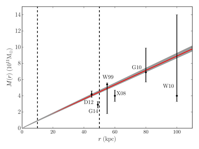
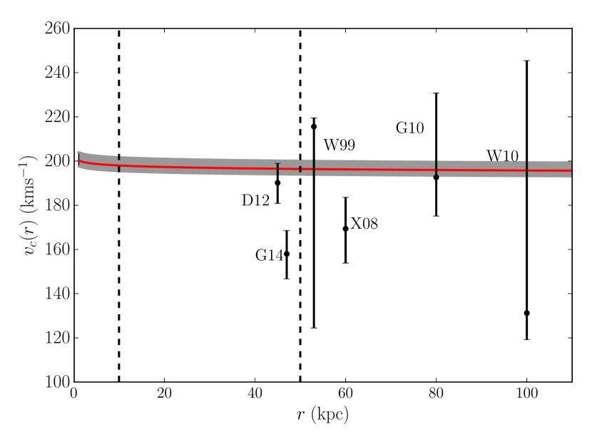
The parameters $v_{0}$, the spherically averaged circular speed at $10{\,\mathrm{kpc}}$, and $\delta$, the slope of the potential, are tightly constrained by our analysis. $v_{0}$ is found to be $\sim 200{\,\mathrm{kms^{-1}}}$, and $\delta$ is very close to zero, implying the rotation curve is almost flat. Taking these results together, we find that the predicted enclosed mass within a spherical shell of radius $50{\,\mathrm{kpc}}$ is $4.48_{-0.14}^{+0.15}\times 10^{11}M_{\odot}$.

Figure 5 depicts the cumulative mass distribution and circular velocity curves of the Milky Way predicted by our model, along with the 68% confidence intervals. We have also plotted the results from other studies on this matter, which we shall now discuss in detail. There are multiple predictions of the Milky Way enclosed mass at $\sim 50{\,\mathrm{kpc}}$. D12 and Xue et al. (2008, hereafter X08) both also use samples of BHB stars from the SDSS: D12 used a subsample of $\sim 1900$ stars from the same dataset considered here, and X08 used a sample from an earlier data release. Our result agrees extremely well with that of D12, who also used distribution function based modelling to place constraints on the mass profile. As one might expect, our error–bar is somewhat smaller, owing to the fact that we use roughly double the amount of data in our study. Interestingly, the logarithmic slope of the potential inferred by D12 is larger than our result: $\delta\sim 0.4$. Their value is almost half–way between the Keplerian and logarithmic cases, so the rotation curve has a steeper decline with radius. This is an interesting result, and has several possible explanations. It is clear that the gravitational potential of the Galaxy cannot possibly be as simple as is implied by Equation (4), and so biases could certainly be introduced into an analysis that assumes such a parameterisation. In particular, if the slope of the Galactic rotation curve changes appreciably over the range of distances between 10 and $50{\,\mathrm{kpc}}$, the lack of flexibility in the model means this cannot be accounted for. D12 only considered stars beyond an elliptical radius $r_{q}=27{\,\mathrm{kpc}}$, the more distant stars in this dataset, so it is not unreasonable to assume that their analysis was more sensitive to the slope of the potential at larger distances. In our case, the left–hand panel of Figure 1 informs us that the majority of the stars reside at radii $10{\,\mathrm{kpc}}\lesssim r\lesssim 25{\,\mathrm{kpc}}$. Therefore, it may possibly be the case that the rotation curve is approximately flat between 10 and $25{\,\mathrm{kpc}}$, but begins to decline more sharply thereafter.

X08 took a rather different approach in their modelling of the BHB population. Rather than fitting analytical distribution functions, they instead compared their data to mock samples drawn from cosmological simulations. Although they also predict a very flat rotation curve, its amplitude is somewhat lower. This discrepancy could be accounted for by the above reasoning, where the circular velocity begins to decline more rapidly with radius.

Wilkinson & Evans (1999, hereafter W99) estimated the mass enclosed at $50{\,\mathrm{kpc}}$ by modelling the distribution of the satellite galaxies and globular clusters of the Milky Way. They used constant anisotropy tracer distribution functions embedded in spherically symmetric models with rotation curves that are flat in the inner parts, then decline in a Keplerian fashion at large radii. These models have a circular velocity of form:

$$v_{\rm c}^{2}=\dfrac{v_{0}^{2}}{\sqrt{1+r^{2}/a^{2}}}.$$ (22)

Their result, $M(r<50{\,\mathrm{kpc}})=5.4^{+0.2}_{-3.6}\times 10^{11}M_{\odot}$, is in excellent agreement with ours (note the asymmetric error–bars). It is also interesting to note that the scale–radius of their model is found to be very large ($140{\,\mathrm{kpc}}\lesssim a\lesssim 260{\,\mathrm{kpc}}$), implying a very flat rotation curve at the distances of the stars in our dataset.

Gibbons et al. (2014) used observations of the Sagittarius stream, in particular the precession of the apocentric position of the stream, to infer the mass profile between radii $50{\,\mathrm{kpc}}<r<100{\,\mathrm{kpc}}$. As the title of their paper states, they find a particularly ‘skinny’ Milky Way, with an enclosed mass at $50{\,\mathrm{kpc}}$ of just $2.9\pm 0.4\times 10^{11}M_{\odot}$. Given the small error bars on their measurement, their result is in tension with ours. Evidently, the two methods possess different systematic biases.

We now compare results from two other studies, Gnedin et al. (2010, hereafter G10) and Watkins et al. (2010, hereafter W10), who both inferred the mass enclosed at larger distances. Although it is still interesting to discuss these results, our result must be extrapolated in order for comparisons to be made. G10 used a large sample of radial velocity measurements of halo stars to carry out a Jeans analysis. They assume a spherically symmetric tracer density with logarithmic slope between -3.5 and -4.5 with a constant anisotropy, and find $M(r<80{\,\mathrm{kpc}})=6.9^{+3.0}_{-1.2}\times 10^{11}M_{\odot}$. In spite of their less sophisticated model for the tracer density, their result is in good agreement with ours. Finally, Watkins et al. (2010) took a sample of 26 satellite galaxies of the Milky Way and applied their virial mass estimators to the data. The estimators assume a power–law tracer density, as well as a power–law gravitational potential. Their measure is very sensitive to the assumed anisotropy of the tracer population, and so their estimate for the enclosed mass has a large error bar. Nonetheless, we are consistent with their conclusions at the 68% confidence level.

Figure 6: Velocity ellipsoids of the best–fit model across a variety of positions. The ellipsoids are everywhere aligned with spherical coordinates, with long axes directed towards the Galactic centre. The size of the ellipsoids do not vary a great deal with radius, suggesting a relatively flat velocity dispersion profile. Their shape becomes more elongated with radius, indicating that the velocity anisotropy of the BHB population is growing with distance from the Galactic centre.

Figure 7: Maps of the velocity dispersions $\sigma_{r}$ (top), $\sigma_{\phi}$ (middle) and $\sigma_{\theta}$ (bottom). The radial and azimuthal velocity dispersion contours are oblate, whereas the latitudinal velocity dispersions are prolate. The radial velocity dispersions decrease the least with Galactocentric distance, and the latitudinal dispersions the most – as we expect for a flattened density.

5.3 Kinematics of the Stellar Halo

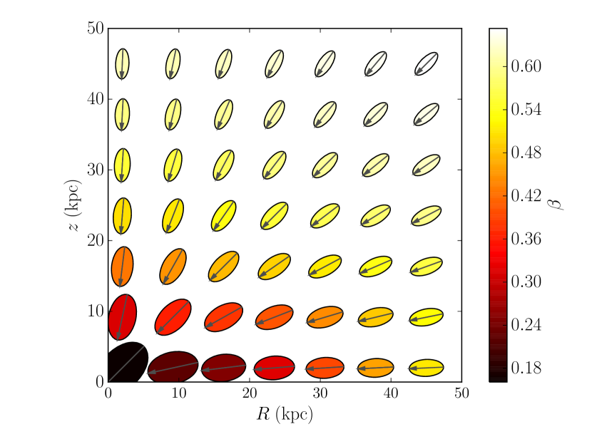
We now study the kinematics of our best–fit model. Figure 6 depicts the velocity ellipsoids of our model over a range of positions in the Galaxy. Our model naturally provides a velocity ellipsoid that is everywhere aligned with spherical coordinates, in agreement with the observations (e.g. Smith et al. 2009, Bond et al. 2010). The ellipsoid always has a long–axis pointing towards the Galactic centre, meaning that the orbital distribution is everywhere radially biased. The ellipsoid becomes more elongated with distance from the Galactic centre, implying that the stellar halo becomes more radially biased in the outskirts. Each ellipse is coloured by the value of the anisotropy parameter

$$\beta(r)=1-\dfrac{\sigma_{\phi}^{2}+\sigma_{\theta}^{2}}{2\sigma_{r}^{2}},$$ (23)

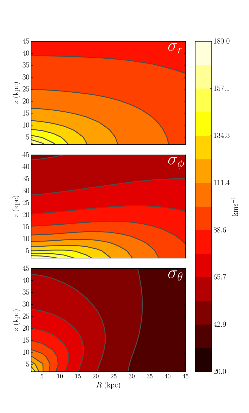
which is a measure of the local velocity anisotropy. If $\beta>0$ ($<0$), then the model is radially (tangentially) biased, and $\beta=0$ implies an isotropic model. Figure 7 depicts maps of the three spherical velocity dispersions with position. We can see that the radial and azimuthal dispersions are oblate, whereas the latitudinal dispersions are prolate in their distribution. The latitudinal dispersions also exhibit a ‘pinching’ in their profile in the equatorial plane. This feature appears generic in radially biased models that are oblate or triaxial (Sanders & Evans, 2015).

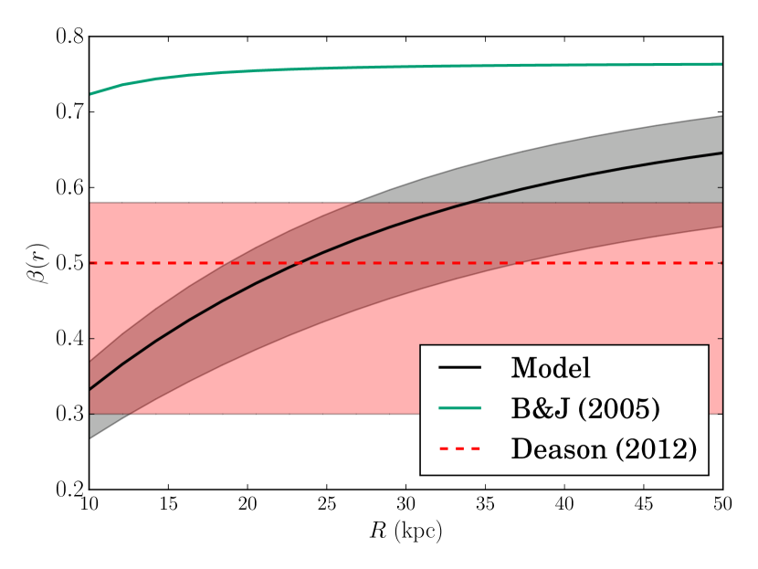
An obvious comparison to make is between the prediction of D12, whose DF enforced a globally constant anisotropy, and that of our model. Figure 8 depicts the anisotropy parameter and its uncertainty as a function of distance along the direction $R=z$ in our model, as well as the value picked out by D12 and their confidence intervals. The two profiles are in agreement within the error bars at all positions for which we have data. Note too that D12’s choice of DFs was questioned by Fermani & Schönrich (2013), but our analysis seems to vindicate the work.

Our model predicts an increasing anisotropy profile with radius, but given the sparsity of the current data, it is difficult to assess how realistic this is, so we turn to numerical simulations to make a comparison. Bullock & Johnston (2005) simulated 11 different stellar haloes in the $\Lambda$CDM context, each with the same dark halo mass and stellar disk at redshift zero, but with distinct accretion histories. The stellar haloes are built up over cosmic time by the accumulation of many different subhaloes which have had stars ‘painted’ onto them. Kafle et al. (2012) then used the Galaxia code (Sharma et al., 2011) to construct synthetic BHB populations for these simulations, and analysed their velocity anisotropy profiles. They find that the mean anisotropy profile of the 11 different BHB populations is well represented by a function

$$\beta(r)=\dfrac{\beta_{0}r^{2}}{r^{2}+r_{0}^{2}},$$ (24)

where $\beta_{0}=0.765$ and $r_{0}=2.4{\,\mathrm{kpc}}$. A rising anisotropy profile is therefore consistent with their findings, although there are significant differences between the simulation properties and those we infer here. We instead find that the anisotropy profile of our model is well represented by the function

$$\beta(r)=\beta_{0}+\dfrac{(\beta_{1}-\beta_{0})r}{r+r_{0}},$$ (25)

with $\beta_{0}=0.05$, $\beta_{1}=0.82$ and $r_{0}=18.2{\,\mathrm{kpc}}$. The anisotropy profile rises at a much lower rate with radius in our model than in the simulations, only reaching $\beta\sim 0.7$ at $r\sim 100{\,\mathrm{kpc}}$. For reference, we also plot the anisotropy profile from the simulations in Figure 8. The differences are curious, since our model is capable of creating profiles similar to that of Equation (24), but they do not seem to be preferred. The Bullock & Johnston (2005) simulations involve many small haloes accreting across cosmic time to build up the stellar halo, but this is by no means the only possibility for the formation history of the Galaxy’s halo.

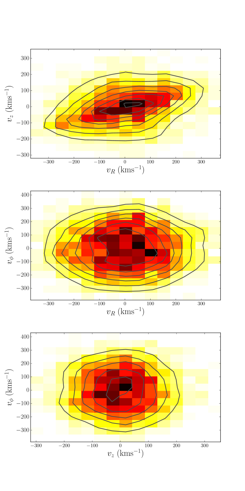
In the future, surveys such as Gaia will provide the three dimensional velocity distributions of halo stars. In fact, such datacubes are already beginning to be available. Bond et al. (2010, hereafter B10) analysed the motion of nearby stars from the SDSS using radial velocities coupled with proper motions derived from SDSS and Palomar Observatory Sky Survey (POSS) astrometry. Figure 9 depicts the two–dimensional velocity distributions of a mock catalogue of 2000 stars drawn from the best–fit model at the position $R=8{\,\mathrm{kpc}}$, $z=3.5{\,\mathrm{kpc}}$. We draw the mock sample using a rejection sampling method, with a sampling distribution that is the product of three broad Gaussians in velocity space. The distributions are qualitatively very similar to those found by B10, although there are some differences (see their Figure 12). The halo distributions presented by B10 are broader in $v_{z}$, which is somewhat surprising given that the halo is a flattened system. Furthermore, B10 infer a greater velocity anisotropy in this region, $\beta\sim 0.65$, as compared with our model, which has $\beta\sim 0.4$. This is perhaps suggestive that the distribution of halo stars is significantly affected by the presence of the disk, which is not accounted for in our model. However, we have not convolved the velocities here with errors, or considered any contamination from disk stars, both of which will have an effect on the observed distributions.

Figure 8: Comparison between the anisotropy predicted by our model (black line, grey shade in 68% confidence intervals), the best–fit value from D12 (dashed red line, red shade in 68% confidence intervals) and the Bullock & Johnston simulations (green line). Our more sophisticated model is in agreement with the analysis of D12 at the 68% confidence level, but inconsistent with the simulated haloes. The simulations are far more radially biased than our model, implying that there may be significant differences between the Milky Way stellar halo formation history and the typical picture assumed in the $\Lambda$CDM paradigm.

Figure 9: The local cylindrical velocity distributions from a mock catalogue at the location $R=8{\,\mathrm{kpc}}$, $z=3.5{\,\mathrm{kpc}}$. We use a simple rejection sampling method to generate a catalogue from our model. Note the tilt of the velocity distribution in the $v_{R}-v_{z}$ projection, which results from the spherical alignment of the velocity ellipsoid.

6 Conclusions

We have presented a new model for the Milky Way stellar halo, and used it to fit a sample of Blue Horizontal Branch stars from the Sloan Digital Sky Survey (Xue et al., 2011). For the first time, we have used a distribution function formulated in terms of the action integrals in the fitting analysis. The density profile generated by this DF is flexible, which allows us to use the results on the SDSS photometry from Deason et al. (2011b) as a prior on the spatial distribution of our BHB dataset. We argue that such a prior is necessary due to the unknown selection function of the data. We then fit three model parameters using the sample of 3534 stars, two corresponding to a simple power–law gravitational potential and one that controls the kinematics of the model.

Our results are consistent with a very flat rotation curve for the Milky Way galaxy, with a mass enclosed at $50{\,\mathrm{kpc}}$ of $4.5\times 10^{11}M_{\odot}$. This is in good agreement with other recent estimates in the literature. The spherically aligned velocity ellipsoid of our model is everywhere radially elongated, with a radial bias that increases with Galactocentric distance as

$$\beta(r)=\beta_{0}+\dfrac{(\beta_{1}-\beta_{0})r}{r+r_{0}},$$ (26)

with $\beta_{0}=0.05$, $\beta_{1}=0.82$ and $r_{0}=18.2{\,\mathrm{kpc}}$. This behaviour qualitatively agrees with results seen in numerical simulations, in that the anisotropy parameter is an increasing function of radius, but our model suggests a much gentler growth of $\beta$ than in the simulations. Given that the model can produce far more radially biased distributions than our maximum–likelihood model, it is interesting that the data do not seem to be consistent with the canonical simulations of stellar halo formation. This is suggestive that the formation history of the stellar halo may be somewhat different from that implied by the models of Bullock & Johnston (2005).

Though our model is the most complex DF yet fitted to data on the stellar halo, it still has some obvious limitations. We have tightly constrained the density profile of the stars in our model so that it is in agreement with past analysis of the stellar halo, a step we unfortunately believe to be necessary owing to the unknown selection function of the data (c.f. Das & Binney, in prep.). Evidently, in applications to datasets provided by Milky Way surveys such as Gaia, we will have a better understanding of the selection function and be able to constrain the spatial and kinematic structure of the stars, as well as the Galactic potential.

Another layer of sophistication can be added to our models in order to account for rotation in the stellar halo. Here, we have presumed that there is no net rotation of the halo, when in reality this score is by no means settled  (e.g., Deason et al., 2011a; Fermani & Schönrich, 2013). One way of introducing a mean azimuthal streaming velocity is by modifying the DF to become  (e.g., Deason et al., 2011a; Binney, 2014)

$$f_{\mathrm{rot}}({\boldsymbol{J}})=\left[\gamma\mathrm{tanh}\left(J_{\phi}/\delta J\right)+(1-\gamma)\right]f({\boldsymbol{J}}),$$ (27)

where $\delta J$ is a small action to avoid discontinuities in the gradient of the DF and $f({\boldsymbol{J}})$ is the original ansatz from Equation (12). The parameter $\gamma$ then takes values between $-1/2$ (maximal retrograde motion) and $1/2$ (maximal prograde rotation). We can then add the extra parameter $\gamma$ to the analysis and search for rotation in the stellar halo.

The model presented here is constructed in a very simple potential, meaning that it is possible to write down an ansatz for a DF with predictable features. However, given the rapid recent developments on action estimation in generic potentials (Binney 2012a, Bovy 2014, Sanders & Binney 2014, Sanders & Binney 2015a), it is now of importance that we develop flexible DFs with well–understood properties in more realistic Galactic potentials. Current models of spheroidal components of galaxies (Williams & Evans 2015, Posti et al. 2015) have been developed to produce certain features in spherical potentials, and even though they can be modified for use in axisymmetric potentials (e.g. Das & Binney, in prep.), their properties are less well understood in this case. Eventually, it will be the case that we simultaneously fit multiple–component Galaxy models (e.g. Piffl et al. 2015) to data from various surveys, but for this to be an effective procedure we must ensure that the DFs used for the various components are sufficiently sophisticated to model the high-quality data that is to appear over the next few years (Perryman et al., 2001). For example, Sanders & Evans (2015) investigate triaxial generalisations of the models in Williams & Evans (2015), which should provide valuable information as to how to progress can be made in this area.

References

- Aihara et al. (2011) Aihara H., et al., 2011, ApJS, 193, 29
- Belokurov et al. (2014) Belokurov V., Koposov S. E., Evans N. W., Peñarrubia J., Irwin M. J., Smith M. C., Lewis G. F., Gieles M., Wilkinson M. I., Gilmore G., Olszewski E. W., Niederste-Ostholt M., 2014, MNRAS, 437, 116
- Binney (1987) Binney J., 1987, in Gilmore G., Carswell B., eds, The Galaxy The Galaxy in action space.. pp 399–412
- Binney (2010) Binney J., 2010, MNRAS, 401, 2318
- Binney (2012a) Binney J., 2012a, MNRAS, 426, 1324
- Binney (2012b) Binney J., 2012b, MNRAS, 426, 1328
- Binney (2014) Binney J., 2014, MNRAS, 440, 787
- Binney & Spergel (1984) Binney J., Spergel D., 1984, MNRAS, 206, 159
- Bond et al. (2010) Bond N. A., et al., 2010, ApJ, 716, 1
- Born (1927) Born M., 1927, The Mechanics of the Atom. G. Bell and Sons
- Bovy (2014) Bovy J., 2014, ApJ, 795, 95
- Bovy (2015) Bovy J., 2015, ApJS, 216, 29
- Bovy & Rix (2013) Bovy J., Rix H.-W., 2013, ApJ, 779, 115
- Bovy et al. (2012) Bovy J., Rix H.-W., Liu C., Hogg D. W., Beers T. C., Lee Y. S., 2012, ApJ, 753, 148
- Bowden et al. (2015) Bowden A., Belokurov V., Evans N. W., 2015, ArXiv e-prints
- Bullock & Johnston (2005) Bullock J. S., Johnston K. V., 2005, ApJ, 635, 931
- de Bruijne et al. (1996) de Bruijne J. H. J., van der Marel R. P., de Zeeuw P. T., 1996, MNRAS, 282, 909
- de Zeeuw (1985) de Zeeuw T., 1985, MNRAS, 216, 273
- Deason et al. (2011a) Deason A. J., Belokurov V., Evans N. W., 2011a, MNRAS, 411, 1480
- Deason et al. (2011b) Deason A. J., Belokurov V., Evans N. W., 2011b, MNRAS, 416, 2903
- Deason et al. (2012) Deason A. J., Belokurov V., Evans N. W., An J., 2012, MNRAS, 424, L44
- Deg & Widrow (2013) Deg N., Widrow L., 2013, MNRAS, 428, 912
- Eddington (1915) Eddington A. S., 1915, MNRAS, 76, 37
- Evans & An (2006) Evans N. W., An J. H., 2006, Phys Rev D, 73, 023524
- Evans et al. (1990) Evans N. W., de Zeeuw P. T., Lynden-Bell D., 1990, MNRAS, 244, 111
- Fermani & Schönrich (2013) Fermani F., Schönrich R., 2013, MNRAS, 432, 2402
- Gibbons et al. (2014) Gibbons S. L. J., Belokurov V., Evans N. W., 2014, MNRAS, 445, 3788
- Gnedin et al. (2010) Gnedin O. Y., Brown W. R., Geller M. J., Kenyon S. J., 2010, ApJL, 720, L108
- Goldstein (1980) Goldstein H., 1980, Classical Mechanics: Second Edition. Addison-Wesley
- Hahn (2005) Hahn T., 2005, Computer Physics Communications, 168, 78
- Henon (1959) Henon M., 1959, Annales d’Astrophysique, 22, 126
- Hunter & de Zeeuw (1992) Hunter C., de Zeeuw P. T., 1992, ApJ, 389, 79
- Hunter & Qian (1993) Hunter C., Qian E., 1993, MNRAS, 262, 401
- Jeans (1919) Jeans J. H., 1919, Problems of cosmogony and stellar dynamics. Cambridge University Press
- Kafle et al. (2012) Kafle P. R., Sharma S., Lewis G. F., Bland-Hawthorn J., 2012, ApJ, 761, 98
- Law & Majewski (2010) Law D. R., Majewski S. R., 2010, ApJ, 714, 229
- Law et al. (2009) Law D. R., Majewski S. R., Johnston K. V., 2009, ApJL, 703, L67
- Nordström et al. (2004) Nordström B., Mayor M., Andersen J., Holmberg J., Pont F., Jørgensen B. R., Olsen E. H., Udry S., Mowlavi N., 2004, AA, 418, 989
- Perryman et al. (2001) Perryman M. A. C., de Boer K. S., Gilmore G., Høg E., Lattanzi M. G., Lindegren L., Luri X., Mignard F., Pace O., de Zeeuw P. T., 2001, AA, 369, 339
- Piffl et al. (2015) Piffl T., Penoyre Z., Binney J., 2015, ArXiv e-prints
- Pila-Díez et al. (2015) Pila-Díez B., de Jong J. T. A., Kuijken K., van der Burg R. F. J., Hoekstra H., 2015, ArXiv e-prints
- Posti et al. (2015) Posti L., Binney J., Nipoti C., Ciotti L., 2015, MNRAS, 447, 3060
- Sanders (2012) Sanders J., 2012, MNRAS, 426, 128
- Sanders & Binney (2014) Sanders J. L., Binney J., 2014, MNRAS, 441, 3284
- Sanders & Binney (2015a) Sanders J. L., Binney J., 2015a, MNRAS, 447, 2479
- Sanders & Binney (2015b) Sanders J. L., Binney J., 2015b, MNRAS, 449, 3479
- Sanders & Evans (2015) Sanders J. L., Evans N. W., 2015, ArXiv e-prints
- Sharma et al. (2011) Sharma S., Bland-Hawthorn J., Johnston K. V., Binney J., 2011, ApJ, 730, 3
- Smith et al. (2009) Smith M. C., Evans N. W., An J. H., 2009, ApJ, 698, 1110
- Smith et al. (2009) Smith M. C., Evans N. W., Belokurov V., Hewett P. C., Bramich D. M., Gilmore G., Irwin M. J., Vidrih S., Zucker D. B., 2009, MNRAS, 399, 1223
- Steinmetz et al. (2006) Steinmetz M., et al., 2006, AJ, 132, 1645
- Vera-Ciro & Helmi (2013) Vera-Ciro C., Helmi A., 2013, ApJL, 773, L4
- Watkins et al. (2010) Watkins L. L., Evans N. W., An J. H., 2010, MNRAS, 406, 264
- Wilkinson & Evans (1999) Wilkinson M. I., Evans N. W., 1999, MNRAS, 310, 645
- Williams & Evans (2015) Williams A. A., Evans N. W., 2015, MNRAS, 448, 1360
- Williams et al. (2014) Williams A. A., Evans N. W., Bowden A. D., 2014, MNRAS, 442, 1405
- Xue et al. (2011) Xue X.-X., Rix H.-W., Yanny B., Beers T. C., Bell E. F., Zhao G., Bullock J. S., Johnston K. V., Morrison H., Rockosi C., Koposov S. E., Kang X., Liu C., Luo A., Lee Y. S., Weaver B. A., 2011, ApJ, 738, 79
- Xue et al. (2008) Xue X. X., Rix H. W., Zhao G., Re Fiorentin P., Naab T., Steinmetz M., van den Bosch F. C., Beers T. C., Lee Y. S., Bell E. F., Rockosi C., Yanny B., Newberg H., Wilhelm R., Kang X., Smith M. C., Schneider D. P., 2008, ApJ, 684, 1143