Global existence and asymptotic behavior of solutions to a nonlocal Fisher-KPP type problem

Shen Bian111Beijing University of Chemical Technology, 100029, Beijing. Email: bianshen66@163.com. Partially supported by China Postdoctoral Science Foundation, No. 2014M560037.    Li Chen222Universität Mannheim, 68131, Mannheim. Email: chen@math.uni-mannheim.de. Partially supported by the National Natural Science Foundation of China (NSFC), No. 11271218.    Evangelos A. Latos333Universität Mannheim, 68131, Mannheim. Email: evangelos.latos@math.uni-mannheim.de.
Abstract

In this work, we consider a nonlocal Fisher-KPP reaction-diffusion problem with Neumann boundary condition and nonnegative initial data in a bounded domain in n(n1)superscript𝑛𝑛1\mathbb{R}^{n}(n\geq 1), with reaction term uα(1m(t))superscript𝑢𝛼1𝑚𝑡u^{\alpha}(1-m(t)), where m(t)𝑚𝑡m(t) is the total mass at time t𝑡t. When α1𝛼1\alpha\geq 1 and the initial mass is greater than or equal to one, the problem has a unique nonnegative classical solution. While if the initial mass is less than one, then the problem admits a unique global solution for n=1,2𝑛12n=1,2 with any 1α<21𝛼21\leq\alpha<2 or n3𝑛3n\geq 3 with any 1α<1+2/n1𝛼12𝑛1\leq\alpha<1+2/n. Moreover, the asymptotic convergence to the solution of the heat equation is proved. Finally, some numerical simulations in dimensions n=1,2𝑛12n=1,2 are exhibited. Especially, for α>2𝛼2\alpha>2 and the initial mass is less than one, our numerical results show that the solution exists globally in time and the mass tends to one as time goes to infinity.

1 Introduction

In this work we consider the following nonlocal initial boundary value problem,

utΔu=uα(1Ωu(x,t)𝑑x),subscript𝑢𝑡Δ𝑢superscript𝑢𝛼1subscriptΩ𝑢𝑥𝑡differential-d𝑥\displaystyle\ u_{t}-\Delta u=u^{\alpha}\left(1-\int_{\Omega}u(x,t)dx\right),\quad xΩ,t>0,formulae-sequence𝑥Ω𝑡0\displaystyle x\in\Omega,t>0, (1a)
uν=0,𝑢𝜈0\displaystyle\ \nabla u\cdot\nu=0, xΩ,𝑥Ω\displaystyle x\in\partial\Omega, (1b)
u(x,0)=u0(x)0,𝑢𝑥0subscript𝑢0𝑥0\displaystyle\ u(x,0)=u_{0}(x)\geq 0,\quad xΩ,𝑥Ω\displaystyle x\in\Omega, (1c)

where u𝑢u is the density, ΩΩ\Omega is a smooth bounded domain in nsuperscript𝑛\mathbb{R}^{n}, n1𝑛1n\geq 1, α1𝛼1\alpha\geq 1 and ν𝜈\nu is the outer unit normal vector on ΩΩ\partial\Omega. Without loss of generality, throughout this paper we assume |Ω|=1Ω1|\Omega|=1 (otherwise, rescale the problem by |Ω|Ω|\Omega|), let m(t)=Ωu(x,t)𝑑x𝑚𝑡subscriptΩ𝑢𝑥𝑡differential-d𝑥m(t)=\int_{\Omega}u(x,t)dx and m0=m(0)subscript𝑚0𝑚0m_{0}=m(0). A damping term with σ>0𝜎0\sigma>0 can also be included to get utΔu+σu=uα(1m(t))subscript𝑢𝑡Δ𝑢𝜎𝑢superscript𝑢𝛼1𝑚𝑡u_{t}-\Delta u+\sigma u=u^{\alpha}(1-m(t)). In this case, similar results to this paper can also be obtained. For simplicity, we assume that σ=0.𝜎0\sigma=0.

In the 1930s, Fisher [16] and Kolmogorov, Petrovskii, Piskunov [24] in population dynamics and Zeldovich, Frank-Kamenetskii [47] in combustion theory started to study problems with this kind of reaction terms. Actually, they introduced the scalar reaction-diffusion equation ut=2ux2+F(u),𝑢𝑡superscript2𝑢superscript𝑥2𝐹𝑢\frac{\partial u}{\partial t}=\frac{\partial^{2}u}{\partial x^{2}}+F(u), and studied the existence, stability and speed of propagation. In the theory of population dynamics, the function F𝐹F is considered as the rate of the reproduction of the population. It is usually of the form

F(u)=βuα(1u)γu.𝐹𝑢𝛽superscript𝑢𝛼1𝑢𝛾𝑢F(u)=\beta u^{\alpha}(1-u)-\gamma u.

From the above model two cases emerge depending on the values of α𝛼\alpha.

In the case of α=1𝛼1\alpha=1, the reproduction rate is proportional to the density u𝑢u of the population and to available resources (1u)1𝑢(1-u). The last term, γu𝛾𝑢-\gamma u, describes the mortality of the population.

The case α=2𝛼2\alpha=2, which is the motivation for our work, considers the addition of sexual reproduction to the model with the reproduction rate proportional to the square of the density, see [42]. For more information on reaction-diffusion waves in biology, we refer to the review paper of Volpert and Petrovskii [41].

Next we pass to the relation between the local and the non-local consumption of resources. In the local reaction-diffusion problem

ut=2ux2+βuα(1u)γu,𝑢𝑡superscript2𝑢superscript𝑥2𝛽superscript𝑢𝛼1𝑢𝛾𝑢\frac{\partial u}{\partial t}=\frac{\partial^{2}u}{\partial x^{2}}+\beta u^{\alpha}(1-u)-\gamma u, (2)

where u𝑢u is the population density, 2ux2superscript2𝑢superscript𝑥2\frac{\partial^{2}u}{\partial x^{2}} describes the random displacement of the individuals of this population and the reaction term represents their reproduction and mortality. Moreover, the reaction term consists of the reproduction term which is represented by the population density to a power, uαsuperscript𝑢𝛼u^{\alpha}, multiplied with the term (1u)1𝑢(1-u) which stands for the local consumption of available resources.

The nonlocal version of the above problem is

ut=2ux2+βuα(1ϕ(xy)u(y,t)𝑑y)γu,𝑢𝑡superscript2𝑢superscript𝑥2𝛽superscript𝑢𝛼1superscriptsubscriptitalic-ϕ𝑥𝑦𝑢𝑦𝑡differential-d𝑦𝛾𝑢\frac{\partial u}{\partial t}=\frac{\partial^{2}u}{\partial x^{2}}+\beta u^{\alpha}\left(1-\int_{-\infty}^{\infty}\phi(x-y)u(y,t)dy\right)-\gamma u, (3)

where β,γ>0𝛽𝛾0\beta,\gamma>0 and ϕ(y)𝑑y=1.superscriptsubscriptitalic-ϕ𝑦differential-d𝑦1\int_{-\infty}^{\infty}\phi(y)dy=1. It can be seen as the case where the individual, located at a certain point, can consume resources in some area around that point. ϕ(xy)italic-ϕ𝑥𝑦\phi(x-y) represents the probability density function that describes the distribution of individuals around their average positions and it depends on the distance from the average point x𝑥x to the actual point y𝑦y. One can easily verify that if ϕitalic-ϕ\phi is a Dirac δ𝛿\delta-function, then the nonlocal problem reduces to (2).

In the current paper we will study problems with reaction terms similar to the above nonlocal reaction terms. There are some already known results on the reaction-diffusion equation with a nonlocal term,

ut=Δu+F(t,u,I(u)),I(u)=Ωu(y,t)𝑑y,formulae-sequencesubscript𝑢𝑡Δ𝑢𝐹𝑡𝑢𝐼𝑢𝐼𝑢subscriptΩ𝑢𝑦𝑡differential-d𝑦u_{t}=\Delta u+F(t,u,I(u)),\quad I(u)=\int_{\Omega}u(y,t)dy,

in a bounded domain ΩΩ\Omega. However, compared to the local version, the results for the nonlocal reaction terms of Fisher-KPP type are relatively limited. Here we list some of the known recent results.

Anguiano, Kloeden and Lorenz considered F=f(u)I(u4)(1I(u4))𝐹𝑓𝑢𝐼superscript𝑢41𝐼superscript𝑢4F=f(u)I(u^{4})(1-I(u^{4})) and proved the existence of a global attractor [1]. Wang and Wo [44] proved the convergence to a stationary solution with F=umI(um),m>1formulae-sequence𝐹superscript𝑢𝑚𝐼superscript𝑢𝑚𝑚1F=u^{m}-I(u^{m}),\ m>1. For F=αeγu+bI(eγu),𝐹𝛼superscript𝑒𝛾𝑢𝑏𝐼superscript𝑒𝛾𝑢F=\alpha e^{\gamma u}+bI(e^{\gamma u}), Pao [33] studied the existence or nonexistence of stationary solutions. Liu, Chen and Lu [28] proved also the blow-up of solutions for a similar equation, see also [14]. Rouchon obtained global estimates of solutions in [37]. For more information on nonlocal KPP-Fisher type problems, we refer to a recent book by Volpert [40].

Nonlocal Fisher-KPP type reaction terms can describe also Darwinian evolution of a structured population density or the behavior of cancer cells with therapy as well as polychemotherapy and chemotherapy, we refer the interested reader to the models found in [29, 30, 31].

Bebernes and Bressan [6] (see also Bebernes [7], Pao[33]) considered the equation with reaction term

F(t,u,I(u))=f(t,u(t,x))+Ωg(t,u(t,y))𝑑y,t>0,xΩ.formulae-sequence𝐹𝑡𝑢𝐼𝑢𝑓𝑡𝑢𝑡𝑥subscriptΩ𝑔𝑡𝑢𝑡𝑦differential-d𝑦formulae-sequence𝑡0𝑥ΩF(t,u,I(u))=f(t,u(t,x))+\int_{\Omega}g(t,u(t,y))dy,\quad t>0,\quad x\in\Omega.

They considered the case when f(t,u)=eu,g(t,u)=keu(k>0)formulae-sequence𝑓𝑡𝑢superscript𝑒𝑢𝑔𝑡𝑢𝑘superscript𝑒𝑢𝑘0f(t,u)=e^{u},\ g(t,u)=ke^{u}\ (k>0), for which the above problem represents an ignition model for a compressible reactive gas, and proved that solutions blow-up.

Later, Wang and Wang [45] considered a power-like nonlinearity, i.e.

F(t,u,I(u))=Ωup(t,y)𝑑ykuq(t,x),t>0,xΩ,formulae-sequence𝐹𝑡𝑢𝐼𝑢subscriptΩsuperscript𝑢𝑝𝑡𝑦differential-d𝑦𝑘superscript𝑢𝑞𝑡𝑥formulae-sequence𝑡0𝑥ΩF(t,u,I(u))=\int_{\Omega}u^{p}(t,y)dy-ku^{q}(t,x),\quad t>0,\quad x\in\Omega,

with p,q>1𝑝𝑞1p,q>1, and proved the blow-up of the solutions.

Budd, Dold and Stuart [11], Hu and Yin [22] considered a similar to the above problem in the case p=2𝑝2p=2 and general p𝑝p respectively,

F(t,u,I(u))=up1|Ω|Ωup(t,y)𝑑y,t>0,xΩ.formulae-sequence𝐹𝑡𝑢𝐼𝑢superscript𝑢𝑝1ΩsubscriptΩsuperscript𝑢𝑝𝑡𝑦differential-d𝑦formulae-sequence𝑡0𝑥ΩF(t,u,I(u))=u^{p}-\frac{1}{|\Omega|}\int_{\Omega}u^{p}(t,y)dy,\quad t>0,\quad x\in\Omega.

With this typical structure, the energy of the solutions is conserved (under Neumann boundary conditions). For this kind of nonlocal problems it is known [45] that there is no comparison principle and they are the closest models to the ones we are considering in this work. For a general study on nonlocal problems, we refer to Quittner’s and Souplet’s book [35] as well as the paper by Souplet [36].

1.1 Preliminary discussion

In this article, we will focus on (1) which has a reaction term of the type

F(t,u,I(u))=uα(1Ωu(x,t)𝑑x)𝐹𝑡𝑢𝐼𝑢superscript𝑢𝛼1subscriptΩ𝑢𝑥𝑡differential-d𝑥F(t,u,I(u))=u^{\alpha}\left(1-\int_{\Omega}u(x,t)dx\right)

for α1𝛼1\alpha\geq 1. One additional fact that makes this problem more difficult to handle is the lack of comparison principle as one can see for example from [45].

For nonnegative u𝑢u, formally by integrating (1) over ΩΩ\Omega, we get,

m(t)=(1m(t))Ωuα𝑑x,superscript𝑚𝑡1𝑚𝑡subscriptΩsuperscript𝑢𝛼differential-d𝑥m^{\prime}(t)=(1-m(t))\int_{\Omega}u^{\alpha}dx,

where m(t)=Ωu(x,t)𝑑x𝑚𝑡subscriptΩ𝑢𝑥𝑡differential-d𝑥m(t)=\int_{\Omega}u(x,t)dx is the total mass at time t𝑡t.

If we start at time t0subscript𝑡0t_{0} such that 1m(t0)<01𝑚subscript𝑡001-m(t_{0})<0, which means that m(t0)>1𝑚subscript𝑡01m(t_{0})>1, we can see that m(t)superscript𝑚𝑡m^{\prime}(t) is negative and therefore m(t)𝑚𝑡m(t) decreases in time. In this case it is natural to expect the global existence of solutions.

On the other hand, if we start at time t0subscript𝑡0t_{0} such that 1m(t0)>01𝑚subscript𝑡001-m(t_{0})>0, we can see that m(t)𝑚𝑡m(t) increases in time. However if (1m(t))1𝑚𝑡(1-m(t)) remains positive, the equation has a similar structure to the heat equation with a power-like reaction term for which we know that the problem might have no global solution for super-critical exponent α<1+2/n𝛼12𝑛\alpha<1+2/n (see for example [4, 5, 18, 19, 20, 23]). In this paper we give a negative answer to this observation. Our main results are the following two theorems:

Theorem 1.

Let n1𝑛1n\geq 1, α1𝛼1\alpha\geq 1 and Ωu0(x)𝑑x=m0>0subscriptΩsubscript𝑢0𝑥differential-d𝑥subscript𝑚00\int_{\Omega}u_{0}(x)dx=m_{0}>0. Assume u0subscript𝑢0u_{0} is nonnegative and u0Lk(Ω)subscript𝑢0superscript𝐿𝑘Ωu_{0}\in L^{k}(\Omega) for any 1<k<1𝑘1<k<\infty. Then for m0<1subscript𝑚01m_{0}<1 with α𝛼\alpha satisfying

1α<1+2/n,1𝛼12𝑛\displaystyle 1\leq\alpha<1+2/n,~{}~{} n3,𝑛3\displaystyle n\geq 3, (4)
1α<2,1𝛼2\displaystyle 1\leq\alpha<2,~{}~{} n=1,2,𝑛12\displaystyle n=1,2, (5)

or m01subscript𝑚01m_{0}\geq 1 with arbitrary α1𝛼1\alpha\geq 1, problem (1) has a unique nonnegative classical solution. Moreover, the following a priori estimates hold true. That’s for m0<1subscript𝑚01m_{0}<1,

u(,t)Lk(Ω)C+Ctk1α1 for anyt>0.subscriptnorm𝑢𝑡superscript𝐿𝑘Ω𝐶𝐶superscript𝑡𝑘1𝛼1 for any𝑡0\displaystyle\|u(\cdot,t)\|_{L^{k}(\Omega)}\leq C+C~{}t^{-\frac{k-1}{\alpha-1}}~{}~{}\mbox{ for any}~{}t>0. (6)

For m01subscript𝑚01m_{0}\geq 1,

uLk(Ω)kC+Ctn(k1)2,n3,formulae-sequencesuperscriptsubscriptnorm𝑢superscript𝐿𝑘Ω𝑘𝐶𝐶superscript𝑡𝑛𝑘12𝑛3\displaystyle\|u\|_{L^{k}(\Omega)}^{k}\leq C+C~{}t^{-\frac{n(k-1)}{2}},\quad n\geq 3, (7)
uLk(Ω)kC+Ct(k1),n=1,2.formulae-sequencesuperscriptsubscriptnorm𝑢superscript𝐿𝑘Ω𝑘𝐶𝐶superscript𝑡𝑘1𝑛12\displaystyle\|u\|_{L^{k}(\Omega)}^{k}\leq C+C~{}t^{-(k-1)},\quad n=1,2. (8)

Here C𝐶C denote different constants depending on m0,k,αsubscript𝑚0𝑘𝛼m_{0},k,\alpha, but not depending on u0Lk(Ω)subscriptnormsubscript𝑢0superscript𝐿𝑘Ω\|u_{0}\|_{L^{k}(\Omega)}.

Theorem 2.

Let u(x,t)𝑢𝑥𝑡u(x,t) be the unique nonnegative classical solution obtained from Theorem 1, v𝑣v be the solution to the heat equation with Neumann boundary condition and initial data Ωv0(x)𝑑x=m0subscriptΩsubscript𝑣0𝑥differential-d𝑥subscript𝑚0\int_{\Omega}v_{0}(x)dx=m_{0}, then as t𝑡t\to\infty,

u(,t)v(,t)(m01)L2(Ω)C1eC2t,subscriptnorm𝑢𝑡𝑣𝑡subscript𝑚01superscript𝐿2Ωsubscript𝐶1superscript𝑒subscript𝐶2𝑡\displaystyle\|u(\cdot,t)-v(\cdot,t)-(m_{0}-1)\|_{L^{2}(\Omega)}\leq C_{1}e^{-C_{2}t}, (9)

where C1,C2subscript𝐶1subscript𝐶2C_{1},C_{2} are constants depending on the initial mass m0subscript𝑚0m_{0} and u0L2α(Ω)subscriptnormsubscript𝑢0superscript𝐿2𝛼Ω\|u_{0}\|_{L^{2\alpha}(\Omega)}.

This paper is organized as follows. In Section 2, we firstly present the dynamics of the mass. The global existence of the solutions and thus the proof the Theorem 1 are shown in Section 3. Section 4 is devoted to the proof of Theorem 2. Section 5 shows the numerical simulations of the problem which give the motivation for our future study for the case α1+2/n𝛼12𝑛\alpha\geq 1+2/n. Finally, Section 6 concludes the main work of our paper, some open questions for problem (1) are also addressed.

2 Dynamics of the total mass

The evolution of the total mass plays the key role in our proof for the global existence of the classical solution. Therefore, we firstly give the evolution of mass Ωu(t)𝑑xsubscriptΩ𝑢𝑡differential-d𝑥\int_{\Omega}u(t)dx in time.

Lemma 3.

For m0>0subscript𝑚00m_{0}>0, the mass Ωu(t)𝑑x=m(t)subscriptΩ𝑢𝑡differential-d𝑥𝑚𝑡\int_{\Omega}u(t)dx=m(t) satisfies

min{1,m0}m(t)max{1,m0}.1subscript𝑚0𝑚𝑡1subscript𝑚0\displaystyle\min\{1,m_{0}\}\leq m(t)\leq\max\{1,m_{0}\}. (10)

Furthermore, we have the following decay estimates

|1m(t)||1m0|emin{1,m0α}t.1𝑚𝑡1subscript𝑚0superscript𝑒1superscriptsubscript𝑚0𝛼𝑡\displaystyle|1-m(t)|\leq|1-m_{0}|e^{-\min\{1,m_{0}^{\alpha}\}t}. (11)

Proof. We return to the original problem (1) and integrate it over ΩΩ\Omega to get:

m(t)=(1m(t))Ωuα𝑑x.superscript𝑚𝑡1𝑚𝑡subscriptΩsuperscript𝑢𝛼differential-d𝑥m^{\prime}(t)=(1-m(t))\int_{\Omega}u^{\alpha}dx. (12)

There are two possibilities depending on the initial mass.

  • If we start at time t0subscript𝑡0t_{0} where 1m(t0)>01𝑚subscript𝑡001-m(t_{0})>0, we can see that m(t)superscript𝑚𝑡m^{\prime}(t) is positive and therefore m𝑚m increases in time. Moreover, with the use of Jensen’s inequality we get by using m(t)m0,𝑚𝑡subscript𝑚0m(t)\geq m_{0},

    m(t)(1m(t))mα(t)(1m(t))m0α.superscript𝑚𝑡1𝑚𝑡superscript𝑚𝛼𝑡1𝑚𝑡superscriptsubscript𝑚0𝛼m^{\prime}(t)\geq(1-m(t))m^{\alpha}(t)\geq(1-m(t))m_{0}^{\alpha}.

    By solving this inequality we get a lower bound on the speed with which m(t)𝑚𝑡m(t) increases to 1 i.e.

    m(t)1em0αt(1m0).𝑚𝑡1superscript𝑒superscriptsubscript𝑚0𝛼𝑡1subscript𝑚0m(t)\geq 1-e^{-m_{0}^{\alpha}t}(1-m_{0}).
  • If 1m(t0)<01𝑚subscript𝑡001-m(t_{0})<0, then m𝑚m decreases in time. By monotonicity, we get m(t)m0𝑚𝑡subscript𝑚0m(t)\leq m_{0} and again by Jensen’s inequality,

    m(t)(1m(t))mα(t)<1m(t),superscript𝑚𝑡1𝑚𝑡superscript𝑚𝛼𝑡1𝑚𝑡m^{\prime}(t)\leq(1-m(t))m^{\alpha}(t)<1-m(t),

    then we get that

    m(t)1+(m01)et.𝑚𝑡1subscript𝑚01superscript𝑒𝑡m(t)\leq 1+(m_{0}-1)e^{-t}.

By putting together the above two cases we have the expected results. \Box

3 Global Existence

This section mainly focuses on the global existence of the classical solution to (1). We will use the following ODE inequality from [9], which was also used in [10].

Lemma 4.

Assume y(t)0𝑦𝑡0y(t)\geq 0 is a C1superscript𝐶1C^{1} function for t>0𝑡0t>0 satisfying

y(t)αβy(t)asuperscript𝑦𝑡𝛼𝛽𝑦superscript𝑡𝑎y^{\prime}(t)\leq\alpha-\beta y(t)^{a}

for a>1,α>0,β>0formulae-sequence𝑎1formulae-sequence𝛼0𝛽0a>1,~{}\alpha>0,~{}\beta>0, then y(t)𝑦𝑡y(t) has the following hyper-contractive property

y(t)(α/β)1/a+[1β(a1)t]1a1 for any t>0.formulae-sequence𝑦𝑡superscript𝛼𝛽1𝑎superscriptdelimited-[]1𝛽𝑎1𝑡1𝑎1 for any 𝑡0\displaystyle y(t)\leq(\alpha/\beta)^{1/a}+\left[\frac{1}{\beta(a-1)t}\right]^{\frac{1}{a-1}}\quad\mbox{ for any ~{}}t>0. (13)

Furthermore, if y(0)𝑦0y(0) is bounded, then

y(t)max(y(0),(α/β)1/a).𝑦𝑡𝑦0superscript𝛼𝛽1𝑎\displaystyle y(t)\leq\max\left(y(0),(\alpha/\beta)^{1/a}\right). (14)

The proof of global existence heavily depends on the following two a priori estimates, Proposition 5 and Proposition 6, and then we will use the compactness arguments to close the proof. Due to the preliminary discussion, we will divide the a priori estimates into two cases m0<1subscript𝑚01m_{0}<1 and m01subscript𝑚01m_{0}\geq 1. Firstly, we focus on m0<1subscript𝑚01m_{0}<1.

Proposition 5.

Let n1𝑛1n\geq 1 and m0<1subscript𝑚01m_{0}<1. If α𝛼\alpha satisfies

1α<1+2/n,1𝛼12𝑛\displaystyle 1\leq\alpha<1+2/n,~{}~{} n3,𝑛3\displaystyle n\geq 3,
1α<2,1𝛼2\displaystyle 1\leq\alpha<2,~{}~{} n=1,2,𝑛12\displaystyle n=1,2,

then for any 1<k<1𝑘1<k<\infty, the nonnegative solution of (1) satisfies

u(,t)Lk(Ω)C(m0,k,α)+C(m0,k,α)tk1α1for anyt>0.subscriptnorm𝑢𝑡superscript𝐿𝑘Ω𝐶subscript𝑚0𝑘𝛼𝐶subscript𝑚0𝑘𝛼superscript𝑡𝑘1𝛼1for any𝑡0\displaystyle\|u(\cdot,t)\|_{L^{k}(\Omega)}\leq C(m_{0},k,\alpha)+C(m_{0},k,\alpha)~{}t^{-\frac{k-1}{\alpha-1}}~{}~{}\mbox{for any}~{}t>0. (15)

Moreover, if u0(x)Lk(Ω)subscript𝑢0𝑥superscript𝐿𝑘Ωu_{0}(x)\in L^{k}(\Omega), then

u(,t)Lk(Ω)max{u0(x)Lk(Ω),C(m0,k,α)},subscriptnorm𝑢𝑡superscript𝐿𝑘Ωsubscriptnormsubscript𝑢0𝑥superscript𝐿𝑘Ω𝐶subscript𝑚0𝑘𝛼\displaystyle\|u(\cdot,t)\|_{L^{k}(\Omega)}\leq\max\left\{\|u_{0}(x)\|_{L^{k}(\Omega)},C(m_{0},k,\alpha)\right\}, (16)

and for any 0<T<0𝑇0<T<\infty

uk2L2(0,T;L2(Ω)).superscript𝑢𝑘2superscript𝐿20𝑇superscript𝐿2Ω\displaystyle\nabla u^{\frac{k}{2}}\in L^{2}\left(0,T;L^{2}(\Omega)\right).

Proof. Since m0<1subscript𝑚01m_{0}<1, by lemma 3 one has m0m(t)1subscript𝑚0𝑚𝑡1m_{0}\leq m(t)\leq 1. Using kuk1𝑘superscript𝑢𝑘1ku^{k-1} as a test function for equation (1) and integrating it by parts

ddtΩuk𝑑x=4(k1)kΩ|uk2|2𝑑x+kΩuk+α1𝑑x(1Ωu𝑑x),𝑑𝑑𝑡subscriptΩsuperscript𝑢𝑘differential-d𝑥4𝑘1𝑘subscriptΩsuperscriptsuperscript𝑢𝑘22differential-d𝑥𝑘subscriptΩsuperscript𝑢𝑘𝛼1differential-d𝑥1subscriptΩ𝑢differential-d𝑥\displaystyle\frac{d}{dt}\int_{\Omega}u^{k}dx=-\frac{4(k-1)}{k}\int_{\Omega}|\nabla u^{\frac{k}{2}}|^{2}dx+k\int_{\Omega}u^{k+\alpha-1}dx\left(1-\int_{\Omega}udx\right),
ddtΩuk𝑑x+4(k1)kΩ|uk2|2𝑑x+km(t)Ωuk+α1𝑑x=kΩuk+α1𝑑x.𝑑𝑑𝑡subscriptΩsuperscript𝑢𝑘differential-d𝑥4𝑘1𝑘subscriptΩsuperscriptsuperscript𝑢𝑘22differential-d𝑥𝑘𝑚𝑡subscriptΩsuperscript𝑢𝑘𝛼1differential-d𝑥𝑘subscriptΩsuperscript𝑢𝑘𝛼1differential-d𝑥\displaystyle\frac{d}{dt}\int_{\Omega}u^{k}dx+\frac{4(k-1)}{k}\int_{\Omega}|\nabla u^{\frac{k}{2}}|^{2}dx+km(t)\int_{\Omega}u^{k+\alpha-1}dx=k\int_{\Omega}u^{k+\alpha-1}dx. (17)

Choosing 1<k<k+α1,1superscript𝑘𝑘𝛼11<k^{\prime}<k+\alpha-1, combining Hölder’s inequality and the Sobolev embedding theorem one has

Ωuk+α1𝑑x=Ωuλk22(k+α1)ku(1λ)k22(k+α1)k𝑑xsubscriptΩsuperscript𝑢𝑘𝛼1differential-d𝑥subscriptΩsuperscript𝑢𝜆𝑘22𝑘𝛼1𝑘superscript𝑢1𝜆𝑘22𝑘𝛼1𝑘differential-d𝑥\displaystyle\int_{\Omega}u^{k+\alpha-1}dx=\int_{\Omega}u^{\lambda\frac{k}{2}\frac{2(k+\alpha-1)}{k}}u^{(1-\lambda)\frac{k}{2}\frac{2(k+\alpha-1)}{k}}dx
\displaystyle\leq uk2Lp(Ω)λ2(k+α1)kuk2L2kk(Ω)(1λ)2(k+α1)ksuperscriptsubscriptnormsuperscript𝑢𝑘2superscript𝐿𝑝Ω𝜆2𝑘𝛼1𝑘superscriptsubscriptnormsuperscript𝑢𝑘2superscript𝐿2superscript𝑘𝑘Ω1𝜆2𝑘𝛼1𝑘\displaystyle\left\|u^{\frac{k}{2}}\right\|_{L^{p}(\Omega)}^{\lambda\frac{2(k+\alpha-1)}{k}}\left\|u^{\frac{k}{2}}\right\|_{L^{\frac{2k^{\prime}}{k}}(\Omega)}^{(1-\lambda)\frac{2(k+\alpha-1)}{k}}
\displaystyle\leq C(k)(uk2L2(Ω)λuk2L2kk(Ω)1λ+uk2L2(Ω)λuk2L2kk(Ω)1λ)2(k+α1)k𝐶𝑘superscriptsuperscriptsubscriptnormsuperscript𝑢𝑘2superscript𝐿2Ω𝜆superscriptsubscriptnormsuperscript𝑢𝑘2superscript𝐿2superscript𝑘𝑘Ω1𝜆superscriptsubscriptnormsuperscript𝑢𝑘2superscript𝐿2Ω𝜆superscriptsubscriptnormsuperscript𝑢𝑘2superscript𝐿2superscript𝑘𝑘Ω1𝜆2𝑘𝛼1𝑘\displaystyle C(k)\left(\left\|\nabla u^{\frac{k}{2}}\right\|_{L^{2}(\Omega)}^{\lambda}\left\|u^{\frac{k}{2}}\right\|_{L^{\frac{2k^{\prime}}{k}}(\Omega)}^{1-\lambda}+\left\|u^{\frac{k}{2}}\right\|_{L^{2}(\Omega)}^{\lambda}\left\|u^{\frac{k}{2}}\right\|_{L^{\frac{2k^{\prime}}{k}}(\Omega)}^{1-\lambda}\right)^{\frac{2(k+\alpha-1)}{k}}
\displaystyle\leq C(k)(uk2L2(Ω)2λ(k+α1)kuk2L2kk(Ω)2(1λ)(k+α1)k+uk2L2(Ω)2λ(k+α1)kuk2L2kk(Ω)2(1λ)(k+α1)k),𝐶𝑘superscriptsubscriptnormsuperscript𝑢𝑘2superscript𝐿2Ω2𝜆𝑘𝛼1𝑘superscriptsubscriptnormsuperscript𝑢𝑘2superscript𝐿2superscript𝑘𝑘Ω21𝜆𝑘𝛼1𝑘superscriptsubscriptnormsuperscript𝑢𝑘2superscript𝐿2Ω2𝜆𝑘𝛼1𝑘superscriptsubscriptnormsuperscript𝑢𝑘2superscript𝐿2superscript𝑘𝑘Ω21𝜆𝑘𝛼1𝑘\displaystyle C(k)\left(\left\|\nabla u^{\frac{k}{2}}\right\|_{L^{2}(\Omega)}^{\frac{2\lambda(k+\alpha-1)}{k}}\left\|u^{\frac{k}{2}}\right\|_{L^{\frac{2k^{\prime}}{k}}(\Omega)}^{\frac{2(1-\lambda)(k+\alpha-1)}{k}}+\left\|u^{\frac{k}{2}}\right\|_{L^{2}(\Omega)}^{\frac{2\lambda(k+\alpha-1)}{k}}\left\|u^{\frac{k}{2}}\right\|_{L^{\frac{2k^{\prime}}{k}}(\Omega)}^{\frac{2(1-\lambda)(k+\alpha-1)}{k}}\right), (18)

where λ𝜆\lambda is the exponent from Hölder’s inequality, i.e.

λ=k2kk2(k+α1)k2k1p(0,1),𝜆𝑘2superscript𝑘𝑘2𝑘𝛼1𝑘2superscript𝑘1𝑝01\displaystyle\lambda=\frac{\frac{k}{2k^{\prime}}-\frac{k}{2(k+\alpha-1)}}{\frac{k}{2k^{\prime}}-\frac{1}{p}}\in(0,1), (19)

and p𝑝p satisfies

{p=2nn2,n3,2(k+α1)k<p<,n=2,p=,n=1.cases𝑝2𝑛𝑛2𝑛32𝑘𝛼1𝑘𝑝𝑛2𝑝𝑛1\displaystyle\left\{\begin{array}[]{ll}p=\frac{2n}{n-2},&n\geq 3,\\ \frac{2(k+\alpha-1)}{k}<p<\infty,&n=2,\\ p=\infty,&n=1.\end{array}\right. (23)

Now we will divide the analysis into three cases n3,n=2formulae-sequence𝑛3𝑛2n\geq 3,n=2 and n=1𝑛1n=1.

For n3𝑛3n\geq 3, p=2nn2𝑝2𝑛𝑛2p=\frac{2n}{n-2} and then

λ=kn2kkn2(k+α1)kn2k+1n2(0,1),𝜆𝑘𝑛2superscript𝑘𝑘𝑛2𝑘𝛼1𝑘𝑛2superscript𝑘1𝑛201\displaystyle\lambda=\frac{\frac{kn}{2k^{\prime}}-\frac{kn}{2(k+\alpha-1)}}{\frac{kn}{2k^{\prime}}+1-\frac{n}{2}}\in(0,1), (24)

with k>max{(n2)(α1)2,1}𝑘𝑛2𝛼121k>\max\left\{\frac{(n-2)(\alpha-1)}{2},1\right\}. Taking k>(α1)n2superscript𝑘𝛼1𝑛2k^{\prime}>\frac{(\alpha-1)n}{2}, simple computations arrive at

2λ(k+α1)k2𝜆𝑘𝛼1𝑘\displaystyle\frac{2\lambda(k+\alpha-1)}{k} =knk+(α1)nknkn2k+1n2<2.absent𝑘𝑛superscript𝑘𝛼1𝑛superscript𝑘𝑛𝑘𝑛2superscript𝑘1𝑛22\displaystyle=\frac{\frac{kn}{k^{\prime}}+\frac{(\alpha-1)n}{k^{\prime}}-n}{\frac{kn}{2k^{\prime}}+1-\frac{n}{2}}<2.

To sum up, for k>max{(α1)n2,1},superscript𝑘𝛼1𝑛21k^{\prime}>\max\left\{\frac{(\alpha-1)n}{2},1\right\}, thanks to the Young’s inequality, from (18) one has

Ωuk+α1𝑑xsubscriptΩsuperscript𝑢𝑘𝛼1differential-d𝑥absent\displaystyle\int_{\Omega}u^{k+\alpha-1}dx\leq k1k2uk2L2(Ω)2+C(k)uk2L2kk(Ω)(1λ)2(k+α1)k11λ(k+α1)k𝑘1superscript𝑘2superscriptsubscriptnormsuperscript𝑢𝑘2superscript𝐿2Ω2𝐶𝑘superscriptsubscriptnormsuperscript𝑢𝑘2superscript𝐿2superscript𝑘𝑘Ω1𝜆2𝑘𝛼1𝑘11𝜆𝑘𝛼1𝑘\displaystyle\frac{k-1}{k^{2}}\left\|\nabla u^{\frac{k}{2}}\right\|_{L^{2}(\Omega)}^{2}+C(k)\left\|u^{\frac{k}{2}}\right\|_{L^{\frac{2k^{\prime}}{k}}(\Omega)}^{(1-\lambda)\frac{2(k+\alpha-1)}{k}\frac{1}{1-\frac{\lambda(k+\alpha-1)}{k}}}
+C(k)uk2L2(Ω)2λ(k+α1)kuk2L2kk(Ω)2(1λ)(k+α1)k.𝐶𝑘superscriptsubscriptnormsuperscript𝑢𝑘2superscript𝐿2Ω2𝜆𝑘𝛼1𝑘superscriptsubscriptnormsuperscript𝑢𝑘2superscript𝐿2superscript𝑘𝑘Ω21𝜆𝑘𝛼1𝑘\displaystyle+C(k)\left\|u^{\frac{k}{2}}\right\|_{L^{2}(\Omega)}^{\frac{2\lambda(k+\alpha-1)}{k}}\left\|u^{\frac{k}{2}}\right\|_{L^{\frac{2k^{\prime}}{k}}(\Omega)}^{\frac{2(1-\lambda)(k+\alpha-1)}{k}}. (25)

Letting

r=(1λ)2(k+α1)k11λ(k+α1)k,𝑟1𝜆2𝑘𝛼1𝑘11𝜆𝑘𝛼1𝑘\displaystyle r=(1-\lambda)\frac{2(k+\alpha-1)}{k}\frac{1}{1-\frac{\lambda(k+\alpha-1)}{k}}, (26)

recalling m(t)m0𝑚𝑡subscript𝑚0m(t)\geq m_{0}, together (17) with (25) we arrive at

ddtΩuk𝑑x+km0Ωuk+α1𝑑x+3(k1)kuk2L2(Ω)2𝑑𝑑𝑡subscriptΩsuperscript𝑢𝑘differential-d𝑥𝑘subscript𝑚0subscriptΩsuperscript𝑢𝑘𝛼1differential-d𝑥3𝑘1𝑘superscriptsubscriptnormsuperscript𝑢𝑘2superscript𝐿2Ω2\displaystyle\frac{d}{dt}\int_{\Omega}u^{k}dx+km_{0}\int_{\Omega}u^{k+\alpha-1}dx+\frac{3(k-1)}{k}\|\nabla u^{\frac{k}{2}}\|_{L^{2}(\Omega)}^{2}
\displaystyle\leq~{} C(k)uLk(Ω)kr2+C(k)uLk(Ω)λ(k+α1)uLk(Ω)(1λ)(k+α1).𝐶𝑘superscriptsubscriptnorm𝑢superscript𝐿superscript𝑘Ω𝑘𝑟2𝐶𝑘superscriptsubscriptnorm𝑢superscript𝐿𝑘Ω𝜆𝑘𝛼1superscriptsubscriptnorm𝑢superscript𝐿superscript𝑘Ω1𝜆𝑘𝛼1\displaystyle C(k)\|u\|_{L^{k^{\prime}}(\Omega)}^{\frac{kr}{2}}+C(k)\|u\|_{L^{k}(\Omega)}^{\lambda(k+\alpha-1)}\|u\|_{L^{k^{\prime}}(\Omega)}^{(1-\lambda)(k+\alpha-1)}. (27)

On the other hand, using Hölder’s inequality with 1<k<k+α11superscript𝑘𝑘𝛼11<k^{\prime}<k+\alpha-1 we have

uLk(Ω)CuLk+α1(Ω)θuL1(Ω)1θ,subscriptnorm𝑢superscript𝐿superscript𝑘Ω𝐶superscriptsubscriptnorm𝑢superscript𝐿𝑘𝛼1Ω𝜃superscriptsubscriptnorm𝑢superscript𝐿1Ω1𝜃\displaystyle\|u\|_{L^{k^{\prime}}(\Omega)}\leq C\|u\|_{L^{k+\alpha-1}(\Omega)}^{\theta}\|u\|_{L^{1}(\Omega)}^{1-\theta}, (28)
uLk(Ω)CuLk+α1(Ω)ηuL1(Ω)1η,subscriptnorm𝑢superscript𝐿𝑘Ω𝐶superscriptsubscriptnorm𝑢superscript𝐿𝑘𝛼1Ω𝜂superscriptsubscriptnorm𝑢superscript𝐿1Ω1𝜂\displaystyle\|u\|_{L^{k}(\Omega)}\leq C\|u\|_{L^{k+\alpha-1}(\Omega)}^{\eta}\|u\|_{L^{1}(\Omega)}^{1-\eta}, (29)

where

θ=(k+α1)(k1)k(k+α2)(0,1),η=(k+α1)(k1)k(k+α2)(0,1).formulae-sequence𝜃𝑘𝛼1superscript𝑘1superscript𝑘𝑘𝛼201𝜂𝑘𝛼1𝑘1𝑘𝑘𝛼201\displaystyle\theta=\frac{(k+\alpha-1)(k^{\prime}-1)}{k^{\prime}(k+\alpha-2)}\in(0,1),~{}~{}\eta=\frac{(k+\alpha-1)(k-1)}{k(k+\alpha-2)}\in(0,1). (30)

Hence

uLk(Ω)kr2superscriptsubscriptnorm𝑢superscript𝐿superscript𝑘Ω𝑘𝑟2\displaystyle\|u\|_{L^{k^{\prime}}(\Omega)}^{\frac{kr}{2}} (CuLk+α1(Ω)θuL1(Ω)1θ)kr2C(m0,k)uLk+α1(Ω)krθ2.absentsuperscript𝐶superscriptsubscriptnorm𝑢superscript𝐿𝑘𝛼1Ω𝜃superscriptsubscriptnorm𝑢superscript𝐿1Ω1𝜃𝑘𝑟2𝐶subscript𝑚0𝑘superscriptsubscriptnorm𝑢superscript𝐿𝑘𝛼1Ω𝑘𝑟𝜃2\displaystyle\leq\left(C\|u\|_{L^{k+\alpha-1}(\Omega)}^{\theta}\|u\|_{L^{1}(\Omega)}^{1-\theta}\right)^{\frac{kr}{2}}\leq C(m_{0},k)\|u\|_{L^{k+\alpha-1}(\Omega)}^{\frac{kr\theta}{2}}. (31)

Taking (27)-(31) into account we obtain that

ddtΩuk𝑑x+km0uLk+α1(Ω)k+α1+3(k1)kuk2L2(Ω)2𝑑𝑑𝑡subscriptΩsuperscript𝑢𝑘differential-d𝑥𝑘subscript𝑚0superscriptsubscriptnorm𝑢superscript𝐿𝑘𝛼1Ω𝑘𝛼13𝑘1𝑘superscriptsubscriptnormsuperscript𝑢𝑘2superscript𝐿2Ω2\displaystyle\frac{d}{dt}\int_{\Omega}u^{k}dx+km_{0}\|u\|_{L^{k+\alpha-1}(\Omega)}^{k+\alpha-1}+\frac{3(k-1)}{k}\|\nabla u^{\frac{k}{2}}\|_{L^{2}(\Omega)}^{2}
\displaystyle\leq~{} C(m0,k)uLk+α1(Ω)krθ2+C(m0,k)uLk+α1(Ω)(k+α1)[λη+(1λ)θ].𝐶subscript𝑚0𝑘superscriptsubscriptnorm𝑢superscript𝐿𝑘𝛼1Ω𝑘𝑟𝜃2𝐶subscript𝑚0𝑘superscriptsubscriptnorm𝑢superscript𝐿𝑘𝛼1Ω𝑘𝛼1delimited-[]𝜆𝜂1𝜆𝜃\displaystyle C(m_{0},k)\|u\|_{L^{k+\alpha-1}(\Omega)}^{\frac{kr\theta}{2}}+C(m_{0},k)\|u\|_{L^{k+\alpha-1}(\Omega)}^{(k+\alpha-1)[\lambda\eta+(1-\lambda)\theta]}. (32)

Here

kr2𝑘𝑟2\displaystyle\frac{kr}{2} =(1λ)(k+α1)11λ(k+α1)k,absent1𝜆𝑘𝛼111𝜆𝑘𝛼1𝑘\displaystyle=(1-\lambda)(k+\alpha-1)\frac{1}{1-\frac{\lambda(k+\alpha-1)}{k}},
k+α1θ𝑘𝛼1𝜃\displaystyle\frac{k+\alpha-1}{\theta} =k+α211k.absent𝑘𝛼211superscript𝑘\displaystyle=\frac{k+\alpha-2}{1-\frac{1}{k^{\prime}}}.

Recalling the definition of θ,η,λ𝜃𝜂𝜆\theta,\eta,\lambda, direct computations show that λη+(1λ)θ<1𝜆𝜂1𝜆𝜃1\lambda\eta+(1-\lambda)\theta<1. For

1α<1+2n,1𝛼12𝑛\displaystyle 1\leq\alpha<1+\frac{2}{n}, (33)

one can derive that

krθ2<k+α1.𝑘𝑟𝜃2𝑘𝛼1\displaystyle\frac{kr\theta}{2}<k+\alpha-1. (34)

Next for n=2𝑛2n=2, 2(k+α1)k<p<2𝑘𝛼1𝑘𝑝\frac{2(k+\alpha-1)}{k}<p<\infty, by proceeding the similar arguments to the case n3𝑛3n\geq 3 from (24) to (32), we obtain that for

1α<22p,1𝛼22𝑝\displaystyle 1\leq\alpha<2-\frac{2}{p}, (35)

(34) holds true. When n=1𝑛1n=1, p=𝑝p=\infty, then for 1α<21𝛼21\leq\alpha<2, (34) also holds true.

Therefore, combining the three cases n3𝑛3n\geq 3, n=2𝑛2n=2 and n=1𝑛1n=1, using Young’s inequality we obtain from (32) that

ddtΩuk𝑑x+km0uLk+α1(Ω)k+α1+3(k1)kuk2L2(Ω)2𝑑𝑑𝑡subscriptΩsuperscript𝑢𝑘differential-d𝑥𝑘subscript𝑚0superscriptsubscriptnorm𝑢superscript𝐿𝑘𝛼1Ω𝑘𝛼13𝑘1𝑘superscriptsubscriptnormsuperscript𝑢𝑘2superscript𝐿2Ω2\displaystyle\frac{d}{dt}\int_{\Omega}u^{k}dx+km_{0}\|u\|_{L^{k+\alpha-1}(\Omega)}^{k+\alpha-1}+\frac{3(k-1)}{k}\|\nabla u^{\frac{k}{2}}\|_{L^{2}(\Omega)}^{2}
\displaystyle\leq~{} km04uLk+α1(Ω)k+α1+km04uLk+α1(Ω)k+α1+C(m0,k).𝑘subscript𝑚04superscriptsubscriptnorm𝑢superscript𝐿𝑘𝛼1Ω𝑘𝛼1𝑘subscript𝑚04superscriptsubscriptnorm𝑢superscript𝐿𝑘𝛼1Ω𝑘𝛼1𝐶subscript𝑚0𝑘\displaystyle\frac{km_{0}}{4}\|u\|_{L^{k+\alpha-1}(\Omega)}^{k+\alpha-1}+\frac{km_{0}}{4}\|u\|_{L^{k+\alpha-1}(\Omega)}^{k+\alpha-1}+C(m_{0},k). (36)

In addition, Hölder’s inequality yields that

(uLk(Ω)k)1+α1k1uLk+α1(Ω)k+α1uL1(Ω)α1k1.superscriptsuperscriptsubscriptnorm𝑢superscript𝐿𝑘Ω𝑘1𝛼1𝑘1superscriptsubscriptnorm𝑢superscript𝐿𝑘𝛼1Ω𝑘𝛼1superscriptsubscriptnorm𝑢superscript𝐿1Ω𝛼1𝑘1\displaystyle\left(\|u\|_{L^{k}(\Omega)}^{k}\right)^{1+\frac{\alpha-1}{k-1}}\leq\|u\|_{L^{k+\alpha-1}(\Omega)}^{k+\alpha-1}\|u\|_{L^{1}(\Omega)}^{\frac{\alpha-1}{k-1}}. (37)

Then using lemma 4, we solve the ODE inequality

ddtΩuk𝑑x+km02uL1(Ω)α1k1(Ωuk𝑑x)1+α1k1C(m0,k)𝑑𝑑𝑡subscriptΩsuperscript𝑢𝑘differential-d𝑥𝑘subscript𝑚02superscriptsubscriptnorm𝑢superscript𝐿1Ω𝛼1𝑘1superscriptsubscriptΩsuperscript𝑢𝑘differential-d𝑥1𝛼1𝑘1𝐶subscript𝑚0𝑘\displaystyle\frac{d}{dt}\int_{\Omega}u^{k}dx+\frac{km_{0}}{2\|u\|_{L^{1}(\Omega)}^{\frac{\alpha-1}{k-1}}}\left(\int_{\Omega}u^{k}dx\right)^{1+\frac{\alpha-1}{k-1}}\leq C(m_{0},k) (38)

to obtain that for any 1<k<1𝑘1<k<\infty,

uLk(Ω)kC(m0,k,α)+[C(m0,k,α)t]k1α1 for anyt>0.superscriptsubscriptnorm𝑢superscript𝐿𝑘Ω𝑘𝐶subscript𝑚0𝑘𝛼superscriptdelimited-[]𝐶subscript𝑚0𝑘𝛼𝑡𝑘1𝛼1 for any𝑡0\displaystyle\|u\|_{L^{k}(\Omega)}^{k}\leq C(m_{0},k,\alpha)+\left[\frac{C(m_{0},k,\alpha)}{t}\right]^{\frac{k-1}{\alpha-1}}~{}~{}\mbox{ for any}~{}t>0. (39)

Furthermore, if u0(x)Lk(Ω)subscript𝑢0𝑥superscript𝐿𝑘Ωu_{0}(x)\in L^{k}(\Omega) for any 1<k<1𝑘1<k<\infty, then taking y(t)=Ωuk𝑑x𝑦𝑡subscriptΩsuperscript𝑢𝑘differential-d𝑥y(t)=\int_{\Omega}u^{k}dx in lemma 4 one has

uLk(Ω)max{u0(x)Lk(Ω),C(m0,k,α)}.subscriptnorm𝑢superscript𝐿𝑘Ωsubscriptnormsubscript𝑢0𝑥superscript𝐿𝑘Ω𝐶subscript𝑚0𝑘𝛼\displaystyle\|u\|_{L^{k}(\Omega)}\leq\max\left\{\|u_{0}(x)\|_{L^{k}(\Omega)},C(m_{0},k,\alpha)\right\}. (40)

Now we integrate (3) from 00 to T𝑇T in time, then we can obtain that for any T>0𝑇0T>0

Ωuk(T)𝑑x+0TΩ|uk2|2𝑑x𝑑t+0TΩuk+α1𝑑x𝑑tΩu0k𝑑x+C(m0,k)T,subscriptΩsuperscript𝑢𝑘𝑇differential-d𝑥superscriptsubscript0𝑇subscriptΩsuperscriptsuperscript𝑢𝑘22differential-d𝑥differential-d𝑡superscriptsubscript0𝑇subscriptΩsuperscript𝑢𝑘𝛼1differential-d𝑥differential-d𝑡subscriptΩsuperscriptsubscript𝑢0𝑘differential-d𝑥𝐶subscript𝑚0𝑘𝑇\displaystyle\int_{\Omega}u^{k}(T)dx+\int_{0}^{T}\int_{\Omega}\left|\nabla u^{\frac{k}{2}}\right|^{2}dxdt+\int_{0}^{T}\int_{\Omega}u^{k+\alpha-1}dxdt\leq\int_{\Omega}u_{0}^{k}dx+C(m_{0},k)T,

from which we derive

uk2L2(0,T;L2(Ω))for anyT>0.formulae-sequencesuperscript𝑢𝑘2superscript𝐿20𝑇superscript𝐿2Ωfor any𝑇0\displaystyle\nabla u^{\frac{k}{2}}\in L^{2}\left(0,T;L^{2}(\Omega)\right)\quad\mbox{for any}~{}T>0.

This completes the proof. \Box

For m01subscript𝑚01m_{0}\geq 1, owing to lemma 3, we know m(t)1𝑚𝑡1m(t)\geq 1 for any t>0𝑡0t>0, thus we have the following result

Proposition 6.

Let n1𝑛1n\geq 1 and α1𝛼1\alpha\geq 1. Assume u0L+1(Ω)subscript𝑢0superscriptsubscript𝐿1Ωu_{0}\in L_{+}^{1}(\Omega) and Ωu0(x)𝑑x=m01subscriptΩsubscript𝑢0𝑥differential-d𝑥subscript𝑚01\int_{\Omega}u_{0}(x)dx=m_{0}\geq 1, Then for any 1<k<1𝑘1<k<\infty, the nonnegative solution of (1) satisfies that for any t>0𝑡0t>0

uLk(Ω)kC(m0,k)+[C(m0,k)t]n(k1)2,n3,formulae-sequencesuperscriptsubscriptnorm𝑢superscript𝐿𝑘Ω𝑘𝐶subscript𝑚0𝑘superscriptdelimited-[]𝐶subscript𝑚0𝑘𝑡𝑛𝑘12𝑛3\displaystyle\|u\|_{L^{k}(\Omega)}^{k}\leq C(m_{0},k)+\left[\frac{C(m_{0},k)}{t}\right]^{\frac{n(k-1)}{2}},\quad n\geq 3, (41)
uLk(Ω)kC(m0,k)+[C(m0,k)t]k1,n=1,2.formulae-sequencesuperscriptsubscriptnorm𝑢superscript𝐿𝑘Ω𝑘𝐶subscript𝑚0𝑘superscriptdelimited-[]𝐶subscript𝑚0𝑘𝑡𝑘1𝑛12\displaystyle\|u\|_{L^{k}(\Omega)}^{k}\leq C(m_{0},k)+\left[\frac{C(m_{0},k)}{t}\right]^{k-1},\quad n=1,2. (42)

Moreover, if u0Lk(Ω)subscript𝑢0superscript𝐿𝑘Ωu_{0}\in L^{k}(\Omega), then

0Ω|uk2|2𝑑x𝑑tΩu0k𝑑x.superscriptsubscript0subscriptΩsuperscriptsuperscript𝑢𝑘22differential-d𝑥differential-d𝑡subscriptΩsuperscriptsubscript𝑢0𝑘differential-d𝑥\displaystyle\int_{0}^{\infty}\int_{\Omega}\left|\nabla u^{\frac{k}{2}}\right|^{2}dxdt\leq\int_{\Omega}u_{0}^{k}dx. (43)

Proof. Recalling lemma 3, we know that if m0>1subscript𝑚01m_{0}>1, then m(t)1𝑚𝑡1m(t)\geq 1 for any t>0𝑡0t>0. Hence the Lksuperscript𝐿𝑘L^{k} estimates (17) can be reduced to

ddtΩuk𝑑x+4(k1)kΩ|uk2|2𝑑x0.𝑑𝑑𝑡subscriptΩsuperscript𝑢𝑘differential-d𝑥4𝑘1𝑘subscriptΩsuperscriptsuperscript𝑢𝑘22differential-d𝑥0\displaystyle\frac{d}{dt}\int_{\Omega}u^{k}dx+\frac{4(k-1)}{k}\int_{\Omega}|\nabla u^{\frac{k}{2}}|^{2}dx\leq 0. (44)

For n1𝑛1n\geq 1, using Hölder’s inequality one has that for any 1<k<1𝑘1<k<\infty, the following estimate holds

uLk(Ω)ksuperscriptsubscriptnorm𝑢superscript𝐿𝑘Ω𝑘\displaystyle\|u\|_{L^{k}(\Omega)}^{k} uLkp2(Ω)kθuL1(Ω)k(1θ)absentsuperscriptsubscriptnorm𝑢superscript𝐿𝑘𝑝2Ω𝑘𝜃superscriptsubscriptnorm𝑢superscript𝐿1Ω𝑘1𝜃\displaystyle\leq\|u\|_{L^{\frac{kp}{2}}(\Omega)}^{k\theta}\|u\|_{L^{1}(\Omega)}^{k(1-\theta)}
=uk2Lp(Ω)2θuL1(Ω)k(1θ),absentsuperscriptsubscriptnormsuperscript𝑢𝑘2superscript𝐿𝑝Ω2𝜃superscriptsubscriptnorm𝑢superscript𝐿1Ω𝑘1𝜃\displaystyle=\|u^{\frac{k}{2}}\|_{L^{p}(\Omega)}^{2\theta}\|u\|_{L^{1}(\Omega)}^{k(1-\theta)}, (45)

where θ=k1k2p𝜃𝑘1𝑘2𝑝\theta=\frac{k-1}{k-\frac{2}{p}} and

{p=2nn2,n3,2<p<,n=2,p=,n=1.cases𝑝2𝑛𝑛2𝑛32𝑝𝑛2𝑝𝑛1\displaystyle\left\{\begin{array}[]{ll}p=\frac{2n}{n-2},&n\geq 3,\\ 2<p<\infty,&n=2,\\ p=\infty,&n=1.\end{array}\right. (49)

Thanks to the Sobolev embedding theorem and Young’s inequality, from (45) one has

(uLk(Ω)k)1θsuperscriptsuperscriptsubscriptnorm𝑢superscript𝐿𝑘Ω𝑘1𝜃\displaystyle\left(\|u\|_{L^{k}(\Omega)}^{k}\right)^{\frac{1}{\theta}} C(n)(uk2L2(Ω)2+uk2L2(Ω)2)uL1(Ω)k(1θ)θabsent𝐶𝑛superscriptsubscriptnormsuperscript𝑢𝑘2superscript𝐿2Ω2superscriptsubscriptnormsuperscript𝑢𝑘2superscript𝐿2Ω2superscriptsubscriptnorm𝑢superscript𝐿1Ω𝑘1𝜃𝜃\displaystyle\leq C(n)\left(\|\nabla u^{\frac{k}{2}}\|_{L^{2}(\Omega)}^{2}+\|u^{\frac{k}{2}}\|_{L^{2}(\Omega)}^{2}\right)\|u\|_{L^{1}(\Omega)}^{\frac{k(1-\theta)}{\theta}}
C(m0,n)uk2L2(Ω)2+C(m0,n)uLk(Ω)kabsent𝐶subscript𝑚0𝑛superscriptsubscriptnormsuperscript𝑢𝑘2superscript𝐿2Ω2𝐶subscript𝑚0𝑛superscriptsubscriptnorm𝑢superscript𝐿𝑘Ω𝑘\displaystyle\leq C(m_{0},n)\|\nabla u^{\frac{k}{2}}\|_{L^{2}(\Omega)}^{2}+C(m_{0},n)\|u\|_{L^{k}(\Omega)}^{k}
C(m0,n)uk2L2(Ω)2+12(uLk(Ω)k)1θ+C(m0,n,k).absent𝐶subscript𝑚0𝑛superscriptsubscriptnormsuperscript𝑢𝑘2superscript𝐿2Ω212superscriptsuperscriptsubscriptnorm𝑢superscript𝐿𝑘Ω𝑘1𝜃𝐶subscript𝑚0𝑛𝑘\displaystyle\leq C(m_{0},n)\|\nabla u^{\frac{k}{2}}\|_{L^{2}(\Omega)}^{2}+\frac{1}{2}\left(\|u\|_{L^{k}(\Omega)}^{k}\right)^{\frac{1}{\theta}}+C(m_{0},n,k). (50)

Plugging the above estimates into (44) yields that

ddtΩuk𝑑x+C(m0,n,k)(Ωuk𝑑x)1θ+C(m0,n,k)uk2L2(Ω)2C(m0,k,n),𝑑𝑑𝑡subscriptΩsuperscript𝑢𝑘differential-d𝑥𝐶subscript𝑚0𝑛𝑘superscriptsubscriptΩsuperscript𝑢𝑘differential-d𝑥1𝜃𝐶subscript𝑚0𝑛𝑘superscriptsubscriptnormsuperscript𝑢𝑘2superscript𝐿2Ω2𝐶subscript𝑚0𝑘𝑛\displaystyle\frac{d}{dt}\int_{\Omega}u^{k}dx+C(m_{0},n,k)\left(\int_{\Omega}u^{k}dx\right)^{\frac{1}{\theta}}+C(m_{0},n,k)\|\nabla u^{\frac{k}{2}}\|_{L^{2}(\Omega)}^{2}\leq C(m_{0},k,n), (51)

solving the ODE inequality we have that for any t>0𝑡0t>0

uLk(Ω)kC(m0,k,n)+[C(m0,k,n)t]n(k1)2,n3,formulae-sequencesuperscriptsubscriptnorm𝑢superscript𝐿𝑘Ω𝑘𝐶subscript𝑚0𝑘𝑛superscriptdelimited-[]𝐶subscript𝑚0𝑘𝑛𝑡𝑛𝑘12𝑛3\displaystyle\|u\|_{L^{k}(\Omega)}^{k}\leq C(m_{0},k,n)+\left[\frac{C(m_{0},k,n)}{t}\right]^{\frac{n(k-1)}{2}},\quad n\geq 3, (52)
uLk(Ω)kC(m0,k,n)+[C(m0,k,n)t]k1,n=1,2.formulae-sequencesuperscriptsubscriptnorm𝑢superscript𝐿𝑘Ω𝑘𝐶subscript𝑚0𝑘𝑛superscriptdelimited-[]𝐶subscript𝑚0𝑘𝑛𝑡𝑘1𝑛12\displaystyle\|u\|_{L^{k}(\Omega)}^{k}\leq C(m_{0},k,n)+\left[\frac{C(m_{0},k,n)}{t}\right]^{k-1},\quad n=1,2. (53)

Moreover, if u0Lk(Ω)subscript𝑢0superscript𝐿𝑘Ωu_{0}\in L^{k}(\Omega), then (44) directly yields

uLk(Ω)u0Lk(Ω).subscriptnorm𝑢superscript𝐿𝑘Ωsubscriptnormsubscript𝑢0superscript𝐿𝑘Ω\displaystyle\|u\|_{L^{k}(\Omega)}\leq\|u_{0}\|_{L^{k}(\Omega)}. (54)

Next integrating (44) from 00 to \infty in time we obtain that

0Ω|uk2|2𝑑x𝑑tΩu0k𝑑x.superscriptsubscript0subscriptΩsuperscriptsuperscript𝑢𝑘22differential-d𝑥differential-d𝑡subscriptΩsuperscriptsubscript𝑢0𝑘differential-d𝑥\displaystyle\int_{0}^{\infty}\int_{\Omega}\left|\nabla u^{\frac{k}{2}}\right|^{2}dxdt\leq\int_{\Omega}u_{0}^{k}dx. (55)

This closes the proof. \Box

Remark 7.

In fact, (41) and (42) also hold true for heat equation, and the uniform boundedness in time of the Lksuperscript𝐿𝑘L^{k} norm depends only on the initial mass, not depends on the initial Lksuperscript𝐿𝑘L^{k} norm.

Now we have obtained the necessary a priori estimates to complete the proof of Theorem 1. It can be proved by standard methods and for the convenience of the reader we mention the key steps in the following. First of all, from the above estimates, we can take k=2𝑘2k=2 and k=2α𝑘2𝛼k=2\alpha in Proposition 5 and 6 to get the estimates for uL2(L2(0,T))subscriptnorm𝑢superscript𝐿2superscript𝐿20𝑇\|\nabla u\|_{L^{2}(L^{2}(0,T))} and utL2(H1(0,T))subscriptnormsubscript𝑢𝑡superscript𝐿2superscript𝐻10𝑇\|u_{t}\|_{L^{2}(H^{-1}(0,T))} for any T>0𝑇0T>0. By Aubin-Lions lemma [21, 43] , we have the strong compactness of u𝑢u in L2superscript𝐿2L^{2} so that the nonlinear terms can be handled. Therefore, the global existence of weak solutions (in the sense of distributions) can be obtained by standard compactness argument. Secondly, from the estimates of the weak solution in Proposition 5 and Proposition 6, the nonlinear term uα(1m(t))Lk([0,T]×Ω)superscript𝑢𝛼1𝑚𝑡superscript𝐿𝑘0𝑇Ωu^{\alpha}(1-m(t))\in L^{k}([0,T]\times\Omega), k>1for-all𝑘1\forall k>1 for any T>0𝑇0T>0. The solution is a strong Wk2,1subscriptsuperscript𝑊21𝑘W^{2,1}_{k} solution from classical parabolic theory, [26, 27]. By Sobolev embedding, we can bootstrap it to get that classical solution. In the end, the uniqueness can be obtained directly from comparison principle [26, 27] since uα1(1m(t))superscript𝑢𝛼11𝑚𝑡u^{\alpha-1}(1-m(t)) is bounded from below. \Box

4 The long time behavior of solutions

As we can see from the above arguments, equation (1) has a unique classical solution. In this section, we will detect the long time behavior of the global solution.

Theorem 8.

Assume u0Lk(Ω)subscript𝑢0superscript𝐿𝑘Ωu_{0}\in L^{k}(\Omega) for any 1<k<1𝑘1<k<\infty. Let u𝑢u be the classical solution to problem (1) and v𝑣v be the solution to the heat equation with Neumann boundary condition and initial data v0subscript𝑣0v_{0} such that Ωv0(x)𝑑x=m0subscriptΩsubscript𝑣0𝑥differential-d𝑥subscript𝑚0\int_{\Omega}v_{0}(x)dx=m_{0}, Then as t𝑡t\to\infty

u(,t)v(,t)(m01)L2(Ω)C1eC2t,subscriptnorm𝑢𝑡𝑣𝑡subscript𝑚01superscript𝐿2Ωsubscript𝐶1superscript𝑒subscript𝐶2𝑡\|u(\cdot,t)-v(\cdot,t)-(m_{0}-1)\|_{L^{2}(\Omega)}\leq C_{1}e^{-C_{2}t},

where the constants C1subscript𝐶1C_{1}, C2subscript𝐶2C_{2} depend on m0subscript𝑚0m_{0} and u0L2α(Ω)subscriptnormsubscript𝑢0superscript𝐿2𝛼Ω\|u_{0}\|_{L^{2\alpha}(\Omega)}.

Proof. The difference between the two equations is

(uv)t+Δ(uv)=uα(1m(t)).subscript𝑢𝑣𝑡Δ𝑢𝑣superscript𝑢𝛼1𝑚𝑡(u-v)_{t}+\Delta(u-v)=u^{\alpha}(1-m(t)).

Let u¯(t)=Ωu(x,t)𝑑x¯𝑢𝑡subscriptΩ𝑢𝑥𝑡differential-d𝑥\overline{u}(t)=\int_{\Omega}u(x,t)dx and v¯(t)=Ωv(x,t)𝑑x¯𝑣𝑡subscriptΩ𝑣𝑥𝑡differential-d𝑥\overline{v}(t)=\int_{\Omega}v(x,t)dx. By (12), we have u¯t=m(t)=(1m(t))Ωuα𝑑xsubscript¯𝑢𝑡superscript𝑚𝑡1𝑚𝑡subscriptΩsuperscript𝑢𝛼differential-d𝑥\overline{u}_{t}=m^{\prime}(t)=(1-m(t))\int_{\Omega}u^{\alpha}dx. v¯t(t)=0subscript¯𝑣𝑡𝑡0\overline{v}_{t}(t)=0 because of v¯(t)=v¯0¯𝑣𝑡subscript¯𝑣0\overline{v}(t)=\overline{v}_{0}. Therefore,

(uv)t(u¯v¯)t+Δ(uv)=uα(1m(t))(1m(t))Ωuα.subscript𝑢𝑣𝑡subscript¯𝑢¯𝑣𝑡Δ𝑢𝑣superscript𝑢𝛼1𝑚𝑡1𝑚𝑡subscriptΩsuperscript𝑢𝛼(u-v)_{t}-(\overline{u}-\overline{v})_{t}+\Delta(u-v)=u^{\alpha}(1-m(t))-(1-m(t))\int_{\Omega}u^{\alpha}.

The standard L2superscript𝐿2L^{2} estimate shows that,

12ddtΩ|(uv)(u¯v¯)|2𝑑x+Ω|(uv)|2𝑑x=(1m(t))Ω[(uαΩuα𝑑y)((uv)(u¯v¯))]𝑑x.12𝑑𝑑𝑡subscriptΩsuperscript𝑢𝑣¯𝑢¯𝑣2differential-d𝑥subscriptΩsuperscript𝑢𝑣2differential-d𝑥1𝑚𝑡subscriptΩdelimited-[]superscript𝑢𝛼subscriptΩsuperscript𝑢𝛼differential-d𝑦𝑢𝑣¯𝑢¯𝑣differential-d𝑥\frac{1}{2}\frac{d}{dt}\int_{\Omega}|(u-v)-(\overline{u}-\overline{v})|^{2}dx+\int_{\Omega}|\nabla(u-v)|^{2}dx=(1-m(t))\int_{\Omega}\left[\Big{(}u^{\alpha}-\int_{\Omega}u^{\alpha}dy\Big{)}\big{(}(u-v)-(\overline{u}-\overline{v})\big{)}\right]dx.

By taking k=2α𝑘2𝛼k=2\alpha in Proposition 5 and Proposition 6, we get

12ddtΩ|(uv)(u¯v¯)|2𝑑x+Ω|(uv)|2𝑑x12𝑑𝑑𝑡subscriptΩsuperscript𝑢𝑣¯𝑢¯𝑣2differential-d𝑥subscriptΩsuperscript𝑢𝑣2differential-d𝑥\displaystyle\frac{1}{2}\frac{d}{dt}\int_{\Omega}|(u-v)-(\overline{u}-\overline{v})|^{2}dx+\int_{\Omega}|\nabla(u-v)|^{2}dx
\displaystyle\leq 12|1m(t)|Ω|(uv)(u¯v¯)|2𝑑x+C|1m(t)|,121𝑚𝑡subscriptΩsuperscript𝑢𝑣¯𝑢¯𝑣2differential-d𝑥𝐶1𝑚𝑡\displaystyle\frac{1}{2}|1-m(t)|\int_{\Omega}|(u-v)-(\overline{u}-\overline{v})|^{2}dx+C|1-m(t)|,

where C𝐶C depend on m0,αsubscript𝑚0𝛼m_{0},\alpha and u0L2α(Ω)subscriptnormsubscript𝑢0superscript𝐿2𝛼Ω\|u_{0}\|_{L^{2\alpha}(\Omega)}. Applying Poincaré inequality and lemma 3, we get

12ddtΩ|(uv)(u¯v¯)|2𝑑x+C(Ω)Ω|(uv)(u¯v¯)|2𝑑x12𝑑𝑑𝑡subscriptΩsuperscript𝑢𝑣¯𝑢¯𝑣2differential-d𝑥𝐶ΩsubscriptΩsuperscript𝑢𝑣¯𝑢¯𝑣2differential-d𝑥\displaystyle\frac{1}{2}\frac{d}{dt}\int_{\Omega}|(u-v)-(\overline{u}-\overline{v})|^{2}dx+C(\Omega)\int_{\Omega}|(u-v)-(\overline{u}-\overline{v})|^{2}dx
\displaystyle\leq CeCtΩ|(uv)(u¯v¯)|2𝑑x+CeCt.𝐶superscript𝑒𝐶𝑡subscriptΩsuperscript𝑢𝑣¯𝑢¯𝑣2differential-d𝑥𝐶superscript𝑒𝐶𝑡\displaystyle Ce^{-Ct}\int_{\Omega}|(u-v)-(\overline{u}-\overline{v})|^{2}dx+Ce^{-Ct}.

From the above ODE we get the following estimate,

Ω|(uv)(u¯v¯)|2𝑑xC1eC2t,subscriptΩsuperscript𝑢𝑣¯𝑢¯𝑣2differential-d𝑥subscript𝐶1superscript𝑒subscript𝐶2𝑡\displaystyle\int_{\Omega}|(u-v)-(\overline{u}-\overline{v})|^{2}dx\leq C_{1}e^{-C_{2}t},

where C1,C2subscript𝐶1subscript𝐶2C_{1},C_{2} are constants depending on m0subscript𝑚0m_{0} and u0L2α(Ω)subscriptnormsubscript𝑢0superscript𝐿2𝛼Ω\|u_{0}\|_{L^{2\alpha}(\Omega)}. Thus completes Theorem 8. \Box

5 Numerical Results

For 1α<2(n=1,2)1𝛼2𝑛121\leq\alpha<2~{}(n=1,2), if m0<1subscript𝑚01m_{0}<1, it has been shown in the previous sections that the solution will exist globally without any restriction on the initial data. An interesting question is whether the solution also exists globally for α>2𝛼2\alpha>2. In the following, we will give a complete numerical study for n=1,2𝑛12n=1,2 with any α1𝛼1\alpha\geq 1.

5.1 Numerical scheme

For the numerical simulation, we consider the 2-dimensional equation in Ω=[0,b]2Ωsuperscript0𝑏2\Omega=[0,b]^{2} with any b>0𝑏0b>0

{ut=Δu+uα(1Ωu𝑑x𝑑y),(x,y)[0,b]×[0,b],t0,u(t=0)=u0(x,y)0,(x,y)[0,b]×[0,b],ux(0,y,t)=ux(b,y,t)=0,uy(x,0,t)=uy(x,b,t)=0.casesformulae-sequencesubscript𝑢𝑡Δ𝑢superscript𝑢𝛼1subscriptdouble-integralΩ𝑢differential-d𝑥differential-d𝑦formulae-sequence𝑥𝑦0𝑏0𝑏𝑡0missing-subexpressionformulae-sequence𝑢𝑡0subscript𝑢0𝑥𝑦0𝑥𝑦0𝑏0𝑏missing-subexpression𝑢𝑥0𝑦𝑡𝑢𝑥𝑏𝑦𝑡0missing-subexpression𝑢𝑦𝑥0𝑡𝑢𝑦𝑥𝑏𝑡0missing-subexpression\displaystyle\left\{\begin{array}[]{ll}u_{t}=\Delta u+u^{\alpha}\left(1-\iint_{\Omega}udxdy\right),~{}~{}(x,y)\in[0,b]\times[0,b],~{}t\geq 0,\\ u(t=0)=u_{0}(x,y)\geq 0,~{}~{}(x,y)\in[0,b]\times[0,b],\\[5.69054pt] \frac{\partial u}{\partial x}(0,y,t)=\frac{\partial u}{\partial x}(b,y,t)=0,\\[5.69054pt] \frac{\partial u}{\partial y}(x,0,t)=\frac{\partial u}{\partial y}(x,b,t)=0.\end{array}\right. (60)

Denote

f(u)=uα(1Ωu𝑑x𝑑y).𝑓𝑢superscript𝑢𝛼1subscriptdouble-integralΩ𝑢differential-d𝑥differential-d𝑦\displaystyle f(u)=u^{\alpha}\left(1-\iint_{\Omega}udxdy\right). (61)

Here an alternating direction implicit difference scheme is applied to construct the numerical computations.

Let hh be the space step and τ𝜏\tau be the time step, N=b/h+1𝑁𝑏1N=b/h+1 is the number of the discrete points, T𝑇T is the final time and K=T/τ+1𝐾𝑇𝜏1K=T/\tau+1. Denote

x(i)=(i1)h,i=1,2,3,,N1,N,formulae-sequence𝑥𝑖𝑖1𝑖123𝑁1𝑁\displaystyle x(i)=(i-1)*h,~{}~{}i=1,2,3,\cdots,N-1,N,
y(j)=(j1)h,j=1,2,3,,N1,N,formulae-sequence𝑦𝑗𝑗1𝑗123𝑁1𝑁\displaystyle y(j)=(j-1)*h,~{}~{}j=1,2,3,\cdots,N-1,N,
t(k)=(k1)τ,k=1,2,,T/τ+1,formulae-sequence𝑡𝑘𝑘1𝜏𝑘12𝑇𝜏1\displaystyle t(k)=(k-1)*\tau,~{}~{}k=1,2,\cdots,T/\tau+1,
Ωh={(x(i),y(j))|1i,jN}.subscriptΩconditional-set𝑥𝑖𝑦𝑗formulae-sequence1𝑖𝑗𝑁\displaystyle\Omega_{h}=\Big{\{}(x(i),y(j))|1\leq i,j\leq N\Big{\}}.

The discrete solution at each time is presented as a matrix ui,jkN×Nsuperscriptsubscript𝑢𝑖𝑗𝑘superscript𝑁𝑁u_{i,j}^{k}\in\mathbb{R}^{N\times N}, where

ui,j=u(x(i),y(j),),1i,jN,formulae-sequencesubscript𝑢𝑖𝑗𝑢𝑥𝑖𝑦𝑗formulae-sequence1𝑖𝑗𝑁\displaystyle u_{i,j}=u\Big{(}x(i),y(j),\cdot\Big{)},~{}~{}1\leq i,j\leq N,
uk=u(,,t(k)),k=1,2,,K.formulae-sequencesuperscript𝑢𝑘𝑢𝑡𝑘𝑘12𝐾\displaystyle u^{k}=u\Big{(}\cdot,\cdot,t(k)\Big{)},~{}~{}k=1,2,\cdots,K.

Next we introduce some notations:
δx2uij=ui+1,j2uij+ui1,jh2,superscriptsubscript𝛿𝑥2subscript𝑢𝑖𝑗subscript𝑢𝑖1𝑗2subscript𝑢𝑖𝑗subscript𝑢𝑖1𝑗superscript2\displaystyle\delta_{x}^{2}u_{ij}=\frac{u_{i+1,j}-2u_{ij}+u_{i-1,j}}{h^{2}},
δy2uij=ui,j+12uij+ui,j1h2.superscriptsubscript𝛿𝑦2subscript𝑢𝑖𝑗subscript𝑢𝑖𝑗12subscript𝑢𝑖𝑗subscript𝑢𝑖𝑗1superscript2\displaystyle\delta_{y}^{2}u_{ij}=\frac{u_{i,j+1}-2u_{ij}+u_{i,j-1}}{h^{2}}.
Refer to caption
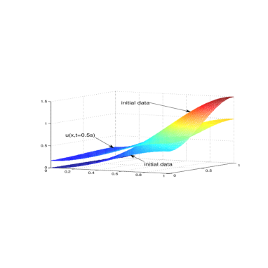
(a) u(x,y)𝑢𝑥𝑦u(x,y) at t=0.5s
Refer to caption
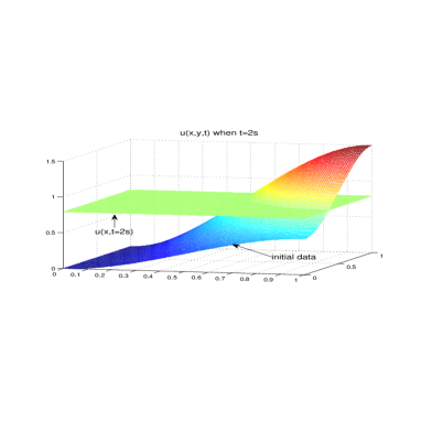
(b) u(x,y)𝑢𝑥𝑦u(x,y) at t=2s
Refer to caption
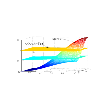
(c) u(x,y)𝑢𝑥𝑦u(x,y) at t=7s
Refer to caption
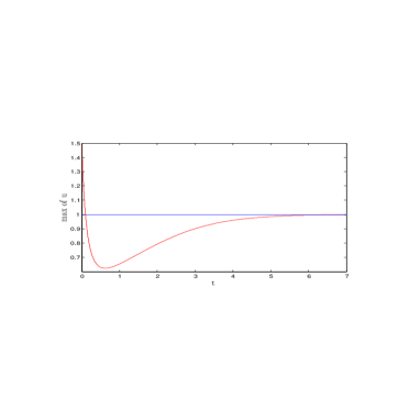
(d) max of u(x,y)𝑢𝑥𝑦u(x,y) with time evolution
Figure 1: u(x,y)𝑢𝑥𝑦u(x,y) with time evolution, initial mass m0<1subscript𝑚01m_{0}<1
Refer to caption
(a) mass of u(x,y)𝑢𝑥𝑦u(x,y) with time evolution
Figure 2: Mass u𝑢u with time evolution, initial mass m0<1subscript𝑚01m_{0}<1
Refer to caption
(a) u𝑢u with time evolution
Refer to caption
(b) max of u𝑢u with time evolution
Figure 3: u(x,y)𝑢𝑥𝑦u(x,y) with time evolution, initial mass m0>1subscript𝑚01m_{0}>1
Refer to caption
(a) Ωu(x,y)𝑑x𝑑ysubscriptdouble-integralΩ𝑢𝑥𝑦differential-d𝑥differential-d𝑦\iint_{\Omega}u(x,y)dxdy with time evolution
Figure 4: Mass of u(x,y)𝑢𝑥𝑦u(x,y) with time evolution, initial mass m0>1subscript𝑚01m_{0}>1
Refer to caption
(a) initial u(x,y)𝑢𝑥𝑦u(x,y)
Refer to caption
(b) u(x,y)𝑢𝑥𝑦u(x,y) at t=104𝑡superscript104t=10^{-4}s
Refer to caption
(c) mass of u(x,y)𝑢𝑥𝑦u(x,y) with time evolution
Refer to caption
(d) max of u(x,y)𝑢𝑥𝑦u(x,y) with time evolution
Figure 5: n=2𝑛2n=2, u(x,y)𝑢𝑥𝑦u(x,y) with time evolution, m0<1subscript𝑚01m_{0}<1
Refer to caption
(a) u(x)𝑢𝑥u(x) with time evolution
Refer to caption
(b) max of u(x)𝑢𝑥u(x) with time evolution
Figure 6: n=1𝑛1n=1, u(x)𝑢𝑥u(x) with time evolution, m0<1subscript𝑚01m_{0}<1
Refer to caption
(a) Ωu(x)𝑑xsubscriptΩ𝑢𝑥differential-d𝑥\int_{\Omega}u(x)dx with time evolution
Figure 7: n=1𝑛1n=1, mass of u(x)𝑢𝑥u(x) with time evolution, initial mass m0<1subscript𝑚01m_{0}<1

We construct the ADI scheme with operator splitting method and using Taylor expansion linearizes f(u)𝑓𝑢f(u) to approximate this semi-linear equation as follows

uijk+1uijkτ=(δx2+δy2)(uijk+1+uijk2)τ4(δx2+1)δy2(uijk+1uijk)superscriptsubscript𝑢𝑖𝑗𝑘1superscriptsubscript𝑢𝑖𝑗𝑘𝜏superscriptsubscript𝛿𝑥2superscriptsubscript𝛿𝑦2superscriptsubscript𝑢𝑖𝑗𝑘1superscriptsubscript𝑢𝑖𝑗𝑘2𝜏4superscriptsubscript𝛿𝑥21superscriptsubscript𝛿𝑦2superscriptsubscript𝑢𝑖𝑗𝑘1superscriptsubscript𝑢𝑖𝑗𝑘\displaystyle\frac{u_{ij}^{k+1}-u_{ij}^{k}}{\tau}=\Big{(}\delta_{x}^{2}+\delta_{y}^{2}\Big{)}\left(\frac{u_{ij}^{k+1}+u_{ij}^{k}}{2}\right)-\frac{\tau}{4}\left(\delta_{x}^{2}+1\right)\delta_{y}^{2}\left(u_{ij}^{k+1}-u_{ij}^{k}\right)
+f(uijk)+uijk+1uijk2f(uijk),,2i,jN1,\displaystyle\quad\quad\quad\quad~{}~{}+f\left(u_{ij}^{k}\right)+\frac{u_{ij}^{k+1}-u_{ij}^{k}}{2}f^{\prime}\left(u_{ij}^{k}\right),~{}~{},2\leq i,j\leq N-1, (62)
ui,j1=U0(x(i),y(j)),1i,jN.formulae-sequencesubscriptsuperscript𝑢1𝑖𝑗subscript𝑈0𝑥𝑖𝑦𝑗formulae-sequence1𝑖𝑗𝑁\displaystyle u^{1}_{i,j}=U_{0}\Big{(}x(i),y(j)\Big{)},~{}~{}1\leq i,j\leq N.

(62) can be rearranged into

[1τ2δx2τ2f(uijk)][1τ2δy2]uijk+1=h(uijk),delimited-[]1𝜏2superscriptsubscript𝛿𝑥2𝜏2superscript𝑓superscriptsubscript𝑢𝑖𝑗𝑘delimited-[]1𝜏2superscriptsubscript𝛿𝑦2superscriptsubscript𝑢𝑖𝑗𝑘1superscriptsubscript𝑢𝑖𝑗𝑘\displaystyle\Big{[}1-\frac{\tau}{2}\delta_{x}^{2}-\frac{\tau}{2}f^{\prime}\left(u_{ij}^{k}\right)\Big{]}\Big{[}1-\frac{\tau}{2}\delta_{y}^{2}\Big{]}u_{ij}^{k+1}=h\left(u_{ij}^{k}\right), (63)
h(uijk)=[1τ2f(uijk)]uijk+τf(uijk)+τ2δx2uijk+[τ24δx2+τ24f(uijk)+τ2]δy2uijk.superscriptsubscript𝑢𝑖𝑗𝑘delimited-[]1𝜏2superscript𝑓superscriptsubscript𝑢𝑖𝑗𝑘superscriptsubscript𝑢𝑖𝑗𝑘𝜏𝑓superscriptsubscript𝑢𝑖𝑗𝑘𝜏2superscriptsubscript𝛿𝑥2superscriptsubscript𝑢𝑖𝑗𝑘delimited-[]superscript𝜏24superscriptsubscript𝛿𝑥2superscript𝜏24superscript𝑓superscriptsubscript𝑢𝑖𝑗𝑘𝜏2superscriptsubscript𝛿𝑦2superscriptsubscript𝑢𝑖𝑗𝑘\displaystyle h\left(u_{ij}^{k}\right)=\Big{[}1-\frac{\tau}{2}f^{\prime}\left(u_{ij}^{k}\right)\Big{]}u_{ij}^{k}+\tau f\left(u_{ij}^{k}\right)+\frac{\tau}{2}\delta_{x}^{2}u_{ij}^{k}+\left[\frac{\tau^{2}}{4}\delta_{x}^{2}+\frac{\tau^{2}}{4}f^{\prime}\left(u_{ij}^{k}\right)+\frac{\tau}{2}\right]\delta_{y}^{2}u_{ij}^{k}.

(63) is equivalent to the following ADI scheme

[1τ2δx2τ2f(uijk)]u¯ij=h(uijk),2iN1,j=2,3,,N1,k=1,2,,K.formulae-sequenceformulae-sequencedelimited-[]1𝜏2superscriptsubscript𝛿𝑥2𝜏2superscript𝑓superscriptsubscript𝑢𝑖𝑗𝑘subscript¯𝑢𝑖𝑗superscriptsubscript𝑢𝑖𝑗𝑘2𝑖𝑁1formulae-sequence𝑗23𝑁1𝑘12𝐾\displaystyle\Big{[}1-\frac{\tau}{2}\delta_{x}^{2}-\frac{\tau}{2}f^{\prime}\left(u_{ij}^{k}\right)\Big{]}\bar{u}_{ij}=h\left(u_{ij}^{k}\right),~{}~{}2\leq i\leq N-1,~{}j=2,3,\cdots,N-1,~{}k=1,2,\cdots,K. (64)
u¯1,j=4u¯2,ju¯3,j3,u¯N,j=4u¯N1,ju¯N2,j3,j=2,3,,N1,formulae-sequencesubscript¯𝑢1𝑗4subscript¯𝑢2𝑗subscript¯𝑢3𝑗3formulae-sequencesubscript¯𝑢𝑁𝑗4subscript¯𝑢𝑁1𝑗subscript¯𝑢𝑁2𝑗3𝑗23𝑁1\displaystyle\bar{u}_{1,j}=\frac{4\bar{u}_{2,j}-\bar{u}_{3,j}}{3},~{}~{}\bar{u}_{N,j}=\frac{4\bar{u}_{N-1,j}-\bar{u}_{N-2,j}}{3},~{}~{}j=2,3,\cdots,N-1, (65)
(1τ2δy2)uijk+1=u¯,2jN1,i=2,3,,N1,k=1,2,,K1,formulae-sequenceformulae-sequence1𝜏2superscriptsubscript𝛿𝑦2superscriptsubscript𝑢𝑖𝑗𝑘1¯𝑢2𝑗𝑁1formulae-sequence𝑖23𝑁1𝑘12𝐾1\displaystyle\Big{(}1-\frac{\tau}{2}\delta_{y}^{2}\Big{)}u_{ij}^{k+1}=\bar{u},~{}~{}2\leq j\leq N-1,~{}i=2,3,\cdots,N-1,~{}k=1,2,\cdots,K-1, (66)
ui,1k+1=4ui,2k+1ui,3k+13,ui,Nk+1=4ui,N1k+1ui,N2k+13,i=2,3,,N1.formulae-sequencesuperscriptsubscript𝑢𝑖1𝑘14superscriptsubscript𝑢𝑖2𝑘1superscriptsubscript𝑢𝑖3𝑘13formulae-sequencesuperscriptsubscript𝑢𝑖𝑁𝑘14superscriptsubscript𝑢𝑖𝑁1𝑘1superscriptsubscript𝑢𝑖𝑁2𝑘13𝑖23𝑁1\displaystyle u_{i,1}^{k+1}=\frac{4u_{i,2}^{k+1}-u_{i,3}^{k+1}}{3},~{}~{}u_{i,N}^{k+1}=\frac{4u_{i,N-1}^{k+1}-u_{i,N-2}^{k+1}}{3},~{}~{}i=2,3,\cdots,N-1. (67)

5.2 Numerical examples

Let Ω=[0,1]2Ωsuperscript012\Omega=[0,1]^{2}. In the numerical study, we will consider three cases:

  1. 1.

    n=2,1<α<2formulae-sequence𝑛21𝛼2n=2,1<\alpha<2, we choose m0<1subscript𝑚01m_{0}<1 and u0Lα(Ω)subscript𝑢0superscript𝐿𝛼Ωu_{0}\in L^{\alpha}(\Omega).

  2. 2.

    n=2,α>2formulae-sequence𝑛2𝛼2n=2,\alpha>2, we choose m0<1subscript𝑚01m_{0}<1 and u0Lα(Ω)subscript𝑢0superscript𝐿𝛼Ωu_{0}\in L^{\alpha}(\Omega), Ωu0α𝑑xsubscriptΩsuperscriptsubscript𝑢0𝛼differential-d𝑥\int_{\Omega}u_{0}^{\alpha}dx is large enough.

  3. 3.

    n=1,α=2formulae-sequence𝑛1𝛼2n=1,\alpha=2, we choose m0<1subscript𝑚01m_{0}<1 and u0Lα(Ω)subscript𝑢0superscript𝐿𝛼Ωu_{0}\in L^{\alpha}(\Omega), Ωu02𝑑xsubscriptΩsuperscriptsubscript𝑢02differential-d𝑥\int_{\Omega}u_{0}^{2}dx is large enough.

Case 1: n=2𝑛2n=2, we choose α=3/2𝛼32\alpha=3/2 and the initial data

u0(x,y)=(2x3+3x2+0.5)(2y3+3y2),Ωu0(x,y)𝑑x𝑑y=0.5<1.formulae-sequencesubscript𝑢0𝑥𝑦2superscript𝑥33superscript𝑥20.52superscript𝑦33superscript𝑦2subscriptdouble-integralΩsubscript𝑢0𝑥𝑦differential-d𝑥differential-d𝑦0.51\displaystyle u_{0}(x,y)=\left(-2x^{3}+3x^{2}+0.5\right)\left(-2y^{3}+3y^{2}\right),~{}~{}\iint_{\Omega}u_{0}(x,y)dxdy=0.5<1. (68)

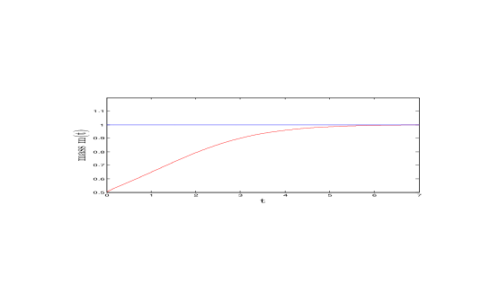
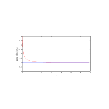
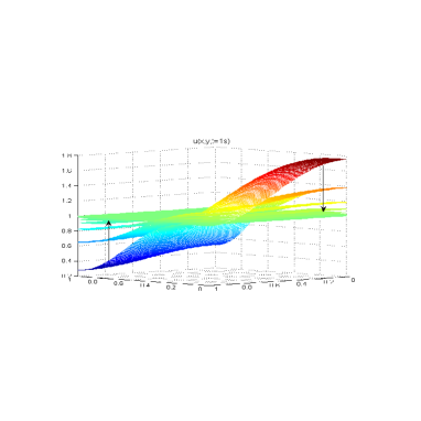
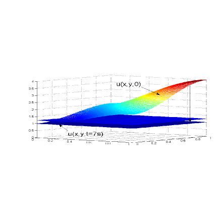
Fig. 1 shows the evolution of the solutions with time. We notice that the solution converges to 1/|Ω|1Ω1/|\Omega|, where |Ω|Ω|\Omega| is the area of the 2-n domain. Fig. 2 shows its corresponding total mass with time evolution. Eventually the mass converges to 1.

For the initial mass is greater than 1, we choose

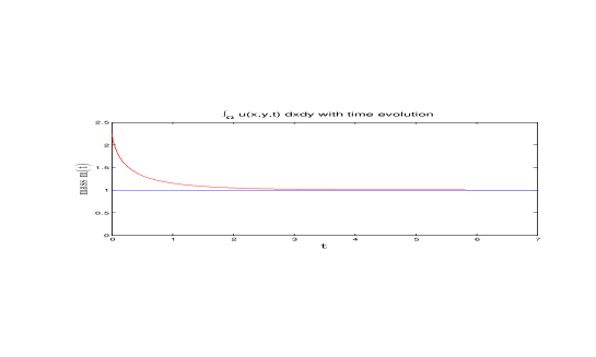
u0(x,y)=(2x3+3x2+1)(2y3+3y2+1),Ωu0(x,y)𝑑x𝑑y=2.25>1.formulae-sequencesubscript𝑢0𝑥𝑦2superscript𝑥33superscript𝑥212superscript𝑦33superscript𝑦21subscriptdouble-integralΩsubscript𝑢0𝑥𝑦differential-d𝑥differential-d𝑦2.251\displaystyle u_{0}(x,y)=\left(-2x^{3}+3x^{2}+1\right)\left(-2y^{3}+3y^{2}+1\right),~{}~{}\iint_{\Omega}u_{0}(x,y)dxdy=2.25>1. (69)

the results are shown in Fig. 3, where the solution converges to 1/|Ω|1Ω1/|\Omega|. The evolution of mass is shown in Fig. 4, we observe that it finally converges to 1.

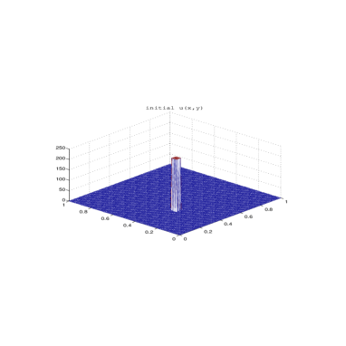
Case 2: n=2𝑛2n=2, α=3𝛼3\alpha=3 and m0<1subscript𝑚01m_{0}<1, the initial data is chosen to be a characteristic function

u={140h2,0.3x0.3+5h,0.3y0.3+5h,0,other,𝑢cases140superscript2formulae-sequence0.3𝑥0.350.3𝑦0.350other\displaystyle u=\left\{\begin{array}[]{ll}\frac{1}{40h^{2}},&0.3\leq x\leq 0.3+5h,~{}0.3\leq y\leq 0.3+5h,\\ 0,&\mbox{other},\end{array}\right.

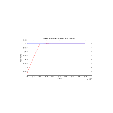
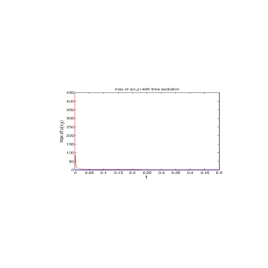
where h=0.010.01h=0.01. Simple computations deduce Ωu0𝑑x=m0=0.625<1subscriptΩsubscript𝑢0differential-d𝑥subscript𝑚00.6251\int_{\Omega}u_{0}dx=m_{0}=0.625<1 and Ωu0α𝑑x=3.9×10⁴subscriptΩsuperscriptsubscript𝑢0𝛼differential-d𝑥3.9superscript104\int_{\Omega}u_{0}^{\alpha}dx=3.9\times 10^{4}. Fig. 5 shows the evolution of the solutions with time. We can notice that the mass tends to one very quickly and u(x,y)𝑢𝑥𝑦u(x,y) goes to 1/|Ω|1Ω1/|\Omega| with time evolution.

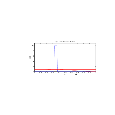
Case 3: n=1𝑛1n=1, α=2𝛼2\alpha=2 and m0<1subscript𝑚01m_{0}<1, the initial data is chosen to be

u={10,0.3x0.35,0,other,𝑢cases100.3𝑥0.350other\displaystyle u=\left\{\begin{array}[]{ll}10,&0.3\leq x\leq 0.35,\\ 0,&\mbox{other},\end{array}\right. (72)

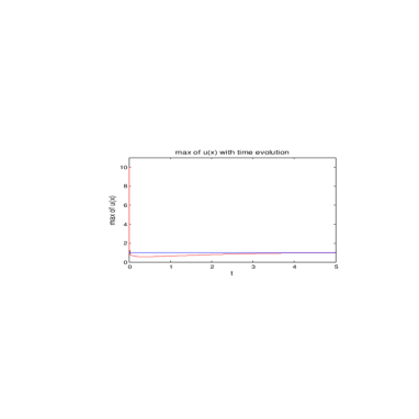
the initial mass m0=0.5subscript𝑚00.5m_{0}=0.5. It can be observed in Fig. 6 that u(x)𝑢𝑥u(x) converges to the constant 1/|Ω|1Ω1/|\Omega|, Fig. 7 shows the mass tends to one finally.

6 Conclusions

This paper concerns the nonlocal Fisher KPP problem (1) with the reaction term’s power α𝛼\alpha. For α1𝛼1\alpha\geq 1, the global existence of a classical solution to (1) is analyzed. When the initial mass is less than one, 1α<21𝛼21\leq\alpha<2 for n=1,2𝑛12n=1,2 or 1α<1+2/n1𝛼12𝑛1\leq\alpha<1+2/n for n3𝑛3n\geq 3, there exists a global unique nonnegative classical solution. When the initial mass is greater than or equal to one, the Fisher KPP problem admits a unique classical solution for any α1𝛼1\alpha\geq 1. Our numerical simulations show that when the initial mass is less than one and α>2𝛼2\alpha>2 for n=1,2𝑛12n=1,2, the unique nonnegative classical solution will exist globally. Therefore, for n=1,2𝑛12n=1,2 with α2𝛼2\alpha\geq 2 or n3𝑛3n\geq 3 with α2/n𝛼2𝑛\alpha\geq 2/n, our conjecture is that the problem (1) also admits a global unique nonnegative classical solution. This is a challenging problem which we will study in the future.

References

  • [1] M. Anguiano, P.E. Kloeden, T. Lorenz. Asymptotic behaviour of nonlocal reaction-diffusion equations. Nonlinear Analysis, 73 (2010), 3044-3057.
  • [2] S. N. Antontsev and M. Chipot, The thermistor problem: Existence, smoothness, unique- ness, blow-up, SIAM J. Math. Anal., 25 (1994), pp. 1128-1156.
  • [3] S. N. Antontsev and M. Chipot, The analysis of blow-up for the thermistor problem, Siberian Math. J., 38 (1997), pp. 827-841.
  • [4] J. M. Ball, Remarks on blow–up and nonexistence theorems for nonlinear evolution equations, Quart. J. Math. Oxford, (2), 28 (1977), 473–486.
  • [5] J. M. Ball, Finite time blow–up in nonlinear problems, Nonlinear Evolution Equations (1977), Academic Press, 189–205.
  • [6] J. W. Bebernes and A. Bressan, Thermal behaviour for a confined reactive gas, J. Differential Equations, 44 (1982), pp. 118-133.
  • [7] J. W. Bebernes and R. Ely, Comparison techniques and the method of lines for a parabolic functional equation, Rocky Mountain J. Math., 12 (1982), pp. 723-733.
  • [8] J. W. Bebernes and P. Talaga, Nonlocal problems modelling shear banding, Comm. Appl. Nonlinear Anal., 3 (1996), pp. 79-103.
  • [9] S. Bian and J.-G. Liu, Dynamic and steady states for multi-dimensional Keller-Segel model with diffusion exponent m>0𝑚0m>0, Comm Math Phy., 323 (2013), 1017-1070.
  • [10] S. Bian, J.-G. Liu and C. Zou, Ultra-contractivity for Keller-Segel model with diffusion exponent m>12/d𝑚12𝑑m>1-2/d, Kinetic and Related Models, 7(1) (2014), 9-28.
  • [11] C. Budd, B. Dold, and A. Stewart, Blowup in a partial differential equation with con- served first integral, SIAM J. Appl. Math., 53 (1993), pp. 718-742.
  • [12] K. Deng, Dynamical behavior of solutions of a semilinear parabolic equation with nonlocal singularity, SIAM J. Math. Anal., 26 (1995), pp. 98-111.
  • [13] K. Deng, M. K. Kwang, and H. A. Levine, The influence of nonlocal nonlinearities on the long time behaviour of solutions of Burgers equation, Quart. Appl. Math., 50 (1992), pp. 173-200.
  • [14] W. Deng, Y. Li, C. Xie. Semilinear reaction-diffusion systems with nonlocal sources, Mathematical and Computer Modelling, 37 (2003), 937-943.
  • [15] M. Fila, Boundedness of global solutions of nonlocal parabolic equations, Nonlinear Anal., 30 (1997), pp. 877-885.
  • [16] Fisher RA. The wave of advance of advantageous genes. Ann Eugenics 1937, (7), 355-69.
  • [17] A. Friedman, “The Porous Medium Equation: Mathematical Theory”, Oxford University Press, 2007.
  • [18] H. Fujita, On the nonlinear equations Δu+eu=0Δ𝑢superscript𝑒𝑢0\Delta u+e^{u}=0 and vt=Δv+evsubscript𝑣𝑡Δ𝑣superscript𝑒𝑣v_{t}=\Delta v+e^{v}, Bull. Amer. Math. Soc., 75 (1969), 132–135.
  • [19] H. Fujita, On some nonexistence and nonuniqueness theorems for nonlinear parabolic equations, Proc. Symp. Pure Math. XVIII, Nonlinear Functional Analysis Amer. Math. Soc., 28 (1970), 105–113.
  • [20] H. Fujita, On the blowing up of solutions of the Cauchy problem for ut=Δu+u1+αsubscript𝑢𝑡Δ𝑢superscript𝑢1𝛼u_{t}=\Delta u+u^{1+\alpha}, J. Fac. Sci. Univ. Tokyo Sect. IA Math. 13 (1966) 109–124.
  • [21] Simon, Jacques. ”Compact sets in the spaceL p (O, T; B).” Annali di Matematica pura ed applicata 146.1 (1986): 65-96.
  • [22] B. Hu and H.–M. Yin, Semilinear parabolic equations with prescribed energy, Rend. Circ. Mat. Palermo, 44 (1995), pp. 479-505.
  • [23] S. Kaplan, On the growth of solutions of quasilinear parabolic equations, Comm. Pure Appl. Math. 16 (1963), 305–330.
  • [24] Kolmogorov AN, Petrovsky IG, Piskunov NS., Investigation of the equation of diffusion combined with increasing of the substance and its application to a biology problem. Bull Moscow State Univ Ser A: Math and Mech 1937;1(6):1-25.
  • [25] A. A. Lacey, Thermal runaway in a non-local problem modelling ohmic heating. I: Model derivation and some special cases, European J. Appl. Math., 6 (1995), pp. 127–144; II: General proofs of blow-up and asymptotics of runaway, European J. Appl. Math., 6 (1995), pp. 201-224.
  • [26] O. A. Ladyzenskaja, V. A. Solonnikov and N. N. Ural’ceva, Linear and Quasilinear Equations of Parabolic Type, Transl. Math. Monog. Vol. 23, Amer. Math. Soc., Providence, R.I., 1968.
  • [27] G.M. Lieberman, Second Order Parabolic Partial Differential Equations, World Scientific, 1996.
  • [28] Q. Liu, Y. Chen, S. Lu. Uniform blow-up profiles for nonlinear and nonlocal reaction-diffusion equations. Nonlinear Analysis, 71 (2009), 1572-1583.
  • [29] Lorz, Alexander and Mirrahimi, Sepideh and Perthame, Benoit, Dirac mass dynamics in multidimensional nonlocal parabolic equations, Commun Part Diff Eq, 2011, vol.36, 6, pa.1071–1098.
  • [30] Lorz, Alexander and Lorenzi, Tommaso and Clairambault, Jean and Escargueil, Alexandre and Perthame, Benoit, Effects of space structure and combination therapies on phenotypic heterogeneity and drug resistance in solid tumors, arXiv:1312.6237v1 [q-bio.TO]
  • [31] Lorz, Alexander and Lorenzi, Tommaso and Hochberg, Michael E and Clairambault, Jean and Perthame, Benoit, Populational adaptive evolution, chemotherapeutic resistance and multiple anti-cancer therapies, ESAIM: M2AN, 2013, vol. 47, 2, p.377–399.
  • [32] A. Lunardi, Analytic Semigroups and Optimal Regularity in Parabolic Problems, Progr. Nonlinear Differential Equations Appl., Birkhäuser- Verlag, 1995.
  • [33] C. V. Pao, Blowing-up of solution for a nonlocal reaction-diffusion problem in combustion theory, J. Math. Anal. Appl., 166 (1992), pp. 591-600.
  • [34] A. Pazy, Semigroups of Linear Operators and Applications to Partial Differential Equations, Appl. Math. Sci., vol. 44, Springer-Verlag, 1983.
  • [35] Pavol Quittner, Philippe Souplet, Superlinear parabolic problems. Blow-up, global existence and steady states, Birkhäuser Advanced Texts, 2007, 584 p.+xi. ISBN: 978-3-7643-8441-8.
  • [36] P. Souplet, Blow-up in nonlocal reaction-diffusion equations, Siam J. Math. Anal. Vol. 29, No. 6, pp. 1301-1334, November 1998.
  • [37] P. Rouchon, Universal bounds for global solutions of a diffusion equation with a nonlocal reaction term, J. Differential Equations, 193 (2003), 75-94.
  • [38] H.B. Stewart, Generation of analytic semigroups by strongly elliptic operators under general boundary conditions, Trans. Amer. Math. Soc. 259 (1) (1980) 299-310.
  • [39] V. Volpert. Elliptic partial differential equations. Volume 1. Fredholm theory of elliptic problems in unbounded domains. Birkhäuser, 2011.
  • [40] V. Volpert. Elliptic partial differential equations. Volume 2. Reaction-diffusion equations. Birkhäuser, 2014.
  • [41] V. Volpert, S. Petrovskii, Reaction-diffusion waves in biology, Physics of Life Reviews 6 (2009) 267-310.
  • [42] V. Volpert, V. Vougalter, Existence of stationary pulses for nonlocal reaction-diffusion equations, preprint.
  • [43] Chen, Xiuqing, Ansgar Jüngel, and Jian-Guo Liu. ”A Note on Aubin-Lions-Dubinski Ä­ Lemmas.” Acta Applicandae Mathematicae (2013): 1-11.
  • [44] X. Wang, W. Wo. Long time behavior of solutions for a scalar nonlocal reaction-diffusion equation. Arch. Math., 96 (2011), 483-490.
  • [45] M. Wang and Y. Wang, Properties of positive solutions for non-local reaction-diffusion problems, Math. Methods Appl. Sci., 19 (1996), pp. 1141-1156.
  • [46] Y. Yin, Quenching for solutions of some parabolic equations with singular nonlocal terms, Dynam. Systems Appl., 5 (1996), pp. 19-30.
  • [47] Zeldovich YaB, Frank-Kamenetskii DA. A theory of thermal propagation of flame. Acta Physicochim USSR 1938;9:341-50.