Measuring the Largest Angular Scale CMB B-mode
Polarization
with Galactic Foregrounds on a Cut Sky
Abstract
We consider the effectiveness of foreground cleaning in the recovery of Cosmic Microwave Background (CMB) polarization sourced by gravitational waves for tensor-to-scalar ratios in the range . Using the planned survey area, frequency bands, and sensitivity of the Cosmology Large Angular Scale Surveyor (CLASS), we simulate maps of Stokes and parameters at 40, 90, 150, and 220 GHz, including realistic models of the CMB, diffuse Galactic thermal dust and synchrotron foregrounds, and Gaussian white noise. We use linear combinations (LCs) of the simulated multifrequency data to obtain maximum likelihood estimates of , the relative scalar amplitude , and LC coefficients. We find that for 10,000 simulations of a CLASS-like experiment using only measurements of the reionization peak (), there is a 95% C.L. upper limit of in the case of no primordial gravitational waves. For simulations with , we recover at 68% C.L. . The reionization peak corresponds to a fraction of the multipole moments probed by CLASS, and simulations including further improve our upper limits to at 95% C.L. ( for primordial gravitational waves with ). In addition to decreasing the current upper bound on by an order of magnitude, these foreground-cleaned low multipole data will achieve a cosmic variance limited measurement of the E-mode polarization’s reionization peak.
Subject headings:
cosmic background radiation – cosmological parameters – early universe – gravitational waves – inflation1. Introduction
All astronomical data on cosmological scales conform to a six-parameter model of the Universe (CDM) with dark matter and a cosmological constant as the dominant components (Hinshaw et al. 2013; Planck Collaboration 2015c). The inflationary paradigm, which postulates a short period of exponential expansion in the early Universe, accounts for features in CDM, including the high degree of homogeneity and flatness and the scalar spectral index (e.g. Guth 1981; Starobinsky 1980; Kazanas 1980; Mukhanov & Chibisov 1981; Einhorn & Sato 1981; Linde 1982; Albrecht & Steinhardt 1982; Hinshaw et al. 2013; Bennett et al. 2013). One of inflation’s predictions is a super-horizon stochastic gravitational wave background that induces polarization in the CMB (Polnarev 1985). We can decompose the CMB’s polarization field into E-modes with parity, and B-modes with parity (Seljak & Zaldarriaga 1997; Kamionkowski et al. 1997; Hu & White 1997). An inflationary B-mode signal can only come from primordial gravitational waves (tensor fluctuations of the metric), so a measurement of such a signal would be strong evidence for an inflationary epoch. We quantify constraints on B-modes in terms of the ratio of tensor fluctuations to scalar (density) fluctuations, , evaluated at . The current upper limit on tensor fluctuations () comes from a combination of Planck and BICEP2 measurements (BICEP2/Keck et al. 2015; Planck Collaboration 2015e).
The Cosmology Large Angular Scale Surveyor (CLASS) is a ground-based experiment that will observe 70% of the sky from Cerro Toco in the Atacama Desert at frequencies of 40, 90, 150, and 220 GHz (Eimer et al. 2012; Essinger-Hileman et al. 2014; Rostem et al. 2014; Appel et al. 2014). First light for the experiment is imminent. CLASS’s band has a projected sensitivity of , an improvement over the Planck map ( at high-, Planck Collaboration 2015a), and will achieve the measurement stability required to reach low multipoles using front end modulation by a variable-delay polarization modulator (VPM) (Chuss et al. 2012). CLASS is currently the only planned sub-orbital mission exploring the combination of frequency and multipole ranges described above. CLASS will probe the reionization peak in the BB power spectrum () along with other missions including PIPER (Lazear et al. 2014), QUIJOTE (López-Caniego et al. 2014), LSPE (Aiola et al. 2012), and GroundBird (Tajima et al. 2012). CLASS will also probe the recombination peak explored by BICEP2 (Ogburn et al. 2010), SPTpol (Austermann et al. 2012), ABS (Essinger-Hileman et al. 2010), ACTPol (Niemack et al. 2010), POLARBEAR (Kermish et al. 2012), EBEX (Oxley et al. 2004), and SPIDER (Filippini et al. 2010). In contrast with other surveys that focus on higher multipoles or have different frequency ranges, CLASS probes a unique combination of frequency and multipole space, as illustrated in Figure 1. In addition to constraining inflation at all of the angular scales where B-modes are predominantly inflationary, we show that a noise-dominated BB spectrum has signal-to-noise that scales as , as opposed to the well-known result found in the cosmic variance limit. In this era of initial measurements of B-mode polarization, we gain more information from large angular scale measurements than conventional wisdom would suggest, as we show in §A.
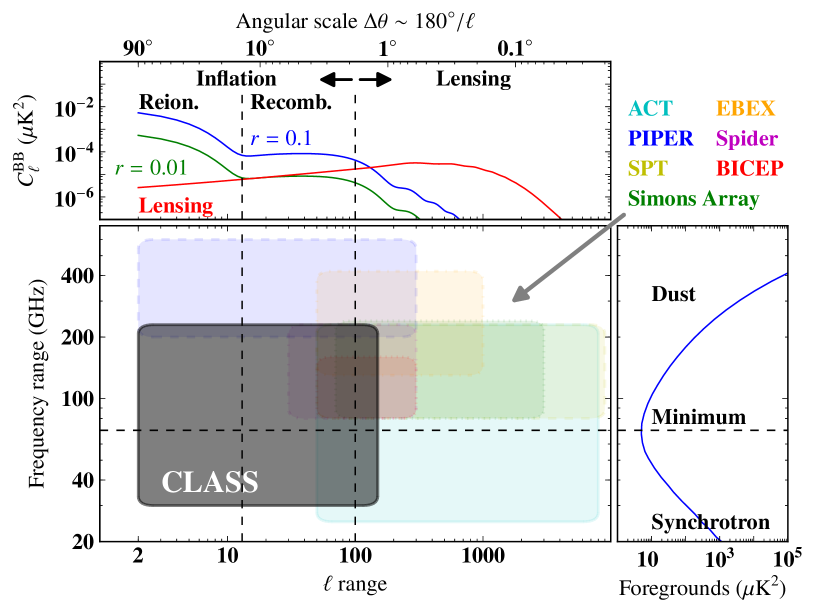
In this paper we explore the recovery of B-modes in the presence of foregrounds, instrument noise, and a cut sky. This analysis will focus on a subset of the simulated CLASS data using only the multipoles , to distill the information available from measurements of the reionization peak alone. In §2 we describe simulations of the CMB with and foreground components in 40, 90, 150, and 220 GHz frequency bands using the CLASS sensitivity and sky coverage. In §3 we describe the maximum likelihood method for recovering the primordial B-mode signal in the presence of foregrounds. We forecast constraints on from this method applied to the simulations in §4.
| Frequency | $\dagger$$\dagger$Values for the amplitude of synchrotron and dust templates at frequency , , come from Equation 2 and assume and . | $\dagger$$\dagger$Values for the amplitude of synchrotron and dust templates at frequency , , come from Equation 2 and assume and . | |||
|---|---|---|---|---|---|
| (GHz) | (K arcmin) | (K arcmin) | (K arcmin) | ||
| 40 | 39 | 1 | 39 | 0.022 | 0.95 |
| 90 | 10 | 0.103 | 4.02 | 0.095 | 4.09 |
| 150 | 15 | 0.032 | 1.25 | 0.306 | 13.2 |
| 220 | 43 | 0.018 | 0.70 | 1 | 43 |
Note. — For each band we list the expected 5-year polarized noise at each frequency (). The columns for show the expected noise contribution in each band when we rescale the 40 and 220 GHz channels according to the synchrotron and dust template scalings used in simulations (Equation 2). The values of are estimated in Essinger-Hileman et al. (2014).
2. Multifrequency Simulations
We use publicly available data to simulate the polarized Galactic synchrotron and dust foregrounds. Our synchrotron map templates are based on the WMAP9 K-band () polarization data (Bennett et al. 2013). Synchrotron polarization dominates the data in this band with negligible contribution from CMB polarization. Our dust polarization templates are based on the Planck maps (Planck Collaboration 2015a). In units of antenna temperature , with the specific intensity, we approximate the modified blackbody emission of dust as a power law with index (Planck Collaboration 2015f) and the synchrotron emission as a power law with (Bennett et al. 2013; Fuskeland et al. 2014). Using these power law indices we rescale the WMAP and Planck data to create templates for synchrotron and dust at 40 and 220 GHz, respectively. The minimum contamination from foregrounds is around 70 GHz (Bennett et al. 2013; Planck Collaboration 2015b), which, along with the location of atmospheric water and oxygen lines, informs the CLASS experiment’s choice of band center frequencies (Eimer et al. 2012).
We estimate CLASS’s sensitivity to tensor modes using random realizations of Gaussian CMB fluctuations with white Gaussian detector noise, all with the same model of foreground contamination. We use the fiducial CDM parameters from WMAP9 (Hinshaw et al. 2013) to simulate the scalar perturbation field, with a tensor contribution added in via . The contribution from gravitational lensing is included in the term. We generate the theoretical spectra using CAMB,111http://camb.info smoothed in multipole space using a Gaussian window function with to reduce aliasing from pixelization. We derive random and maps from the theoretical values using the Healpix package synfast (Górski et al. 2005) with pixels at resolution (),222Healpix maps have resolutions denoted . Each of the 12 lowest resolution pixels that characterize divides into regions where , and the total number of pixels is with characteristic pixel size . The full documentation is at http://healpix.sf.net. including multipoles . We then add dust and synchrotron polarization to each band, along with white Gaussian noise corresponding to the experiment sensitivity, given here in units of K arcmin (see Table 1).
Given CLASS’s wide scan strategy from its site in the Atacama Desert at latitude (Essinger-Hileman et al. 2014), we include data with declination so that . We mask out the Galactic equator based on the WMAP P06 mask, defined in Page et al. (2007), resulting in a final .
We define the polarization maps as a vector with the and Stokes parameters as components. We use and as the synchrotron and dust templates at and respectively, and the simulated CMB. This allows us to generate the simulated multifrequency CLASS polarization data,
| (1) |
where contains the Gaussian white noise maps for and , with the amplitude of the noise determined by the survey sensitivity given in Table 1 (Essinger-Hileman et al. 2014). Because we define the power law spectral indices in terms of antenna temperature and our data are in units of thermodynamic temperature, we scale the foreground channels using the factor
| (2) |
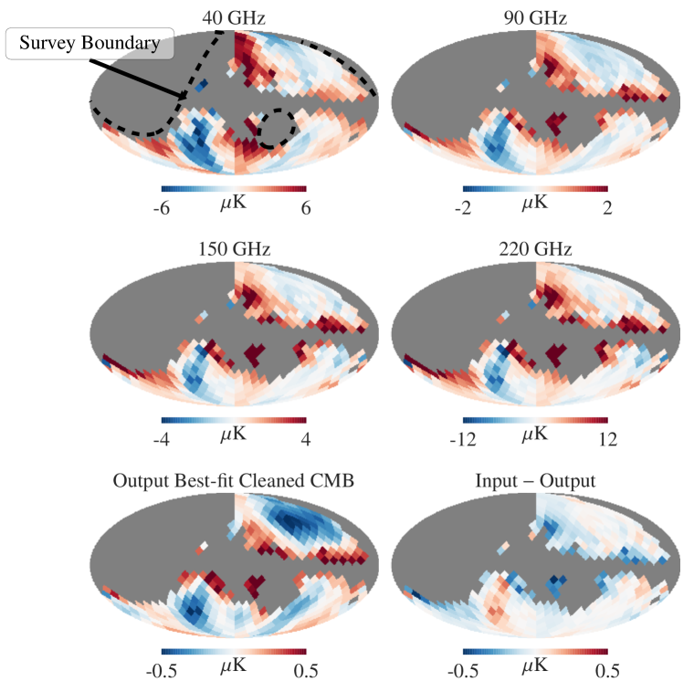
with the conversion factor from thermodynamic to antenna temperatures with . These give the relative strength of each foreground component normalized by its strength at template frequencies . As described above these templates are based on the WMAP K-band for synchrotron and Planck 353 GHz band for dust scaled to and , respectively. For these chosen frequencies and spectral indices, these strengths are and at while for , we have and , as shown in Table 1. We display sample maps of our simulated CLASS data in Figure 2, along with the best-fit cleaned data and the residuals, to be described in §3.
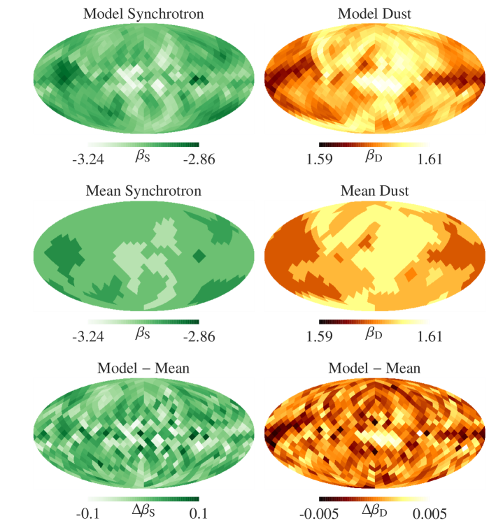
The spatial dependence of the spectral indices is based on the pre-flight Planck Sky Model (PSM) (Delabrouille et al. 2013), which we display in Figure 3. As we demonstrate below, the PSM is consistent with current data. The from this model come from intensity measurements of foreground components, and are not expected to be the same as the polarized power law indices. For this work, we rescale the PSM spectral indices to have mean values and . The amplitude of synchrotron spectral index fluctuations in the WMAP estimate derived from the K and Ka band data (Bennett et al. 2013; Fuskeland et al. 2014) is broadly consistent with the variation in the PSM’s (Miville-Deschênes et al. 2008, model 4). The variation in the dust spectral index has variation (Planck Collaboration 2015f) that is consistent with a constant spectral index (see §B) and hence with the small variation in the PSM (Finkbeiner et al. 1999, model 8). Note that we only use the pre-flight PSM for spectral variation, while we derive the 40 and 220 GHz polarization templates from WMAP and Planck data respectively, as described above. However, the CLASS dataset itself will improve on this and be used in our final analysis.
In this study we focus on the effects of foregrounds and a cut sky on the recoverability of primordial B-modes. To isolate these effects we do not include potential instrumental systematics. For measurements that use a VPM to suppress noise, Miller et al. (2015) find that B-mode power from systematic effects can be suppressed to levels below the primordial level for , which suggests such effects are negligible in the context of this work.
3. Pixelized Likelihood Analysis
We base our analysis on methods developed in Efstathiou (2006) and Katayama & Komatsu (2011), and extend the Gaussian likelihood formalism to an arbitrary number of frequency channels, each with its own linear fit coefficient. We define the likelihood
| (3) |
where
| (4) |
is the CMB map cleaned using frequency channels, with preserving the CMB’s frequency spectrum. We achieve this constraint defining as . We define the pixel-space covariance matrix,
| (5) |
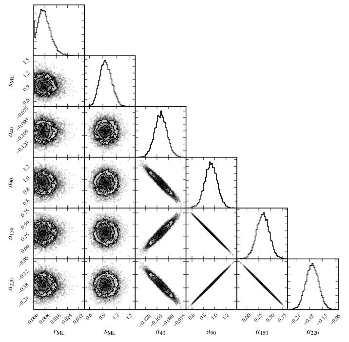
Here is the identity matrix in pixel space, and is the survey noise. The ’s are the theoretical signal covariance matrices, which themselves come from the power spectra, and , assuming uncorrelated E- and B-modes, as detailed in Appendix A of Katayama & Komatsu (2011). We vary , the amplitude of scalar fluctuations normalized by a fiducial value, to mitigate spurious correlations between the CMB and foregrounds in the maximum likelihood fitting as in §5.1 of Katayama & Komatsu (2011). We use uniform unbounded priors on all parameters except for the tensor-to-scalar ratio and the 40 GHz and 220 GHz coefficients. We impose the prior to avoid singular covariance matrices in Equation 5, and we impose the prior that the 40 and 220 GHz coefficients are negative to avoid numerical errors (which does not affect our overall results, as seen in Figure 4). The product of our likelihood and priors is proportional to the Bayesian posterior probability distribution for our parameters. We emphasize that this method differs from the internal linear combination method described in Efstathiou et al. (2009) due to our simultaneous variation of cosmological and foreground LC parameters and also due to the presence of the weighting for the solution of LC coefficients. When we maximize the likelihood (Equation 3) using the covariance matrix (Equation 5), the maximum likelihood LC coefficients, , we create a map, , that best approximates a realization of the CMB with Gaussian noise. The modified foreground removal method is effective because the pixel-pixel correlations, , drive the fit so that the mean of the map, , is zero, with variance corresponding to CMB fluctuations and instrumental white noise.
We obtain an estimate of the CMB, , by finding the parameters , , , , , and that maximize the likelihood with the priors and . We find that although a Monte Carlo Markov Chain (MCMC) estimation gives posterior distributions and suitable estimators for these parameters, using the scipy minimization routine fmin_l_bfgs_b, an implementation of the limited-memory Broyden-Fletcher-Goldfarb-Shanno (BFGS) algorithm (Byrd et al. 1995), gives estimates of the maximum likelihood values for parameters at a fraction of the time required to compute the full MCMC posterior distributions. We plan to use MCMC methods for the analysis of the actual multi-frequency CLASS observed maps, but cosmic variance can cause different posterior distributions for the same underlying value of . For our simulations with random realizations of CMB and noise, the distribution of maximum likelihood values for is comparable to the width of the posterior distribution of a single Monte Carlo chain. For forecasting purposes, we therefore run large numbers of simulations and study the posterior distribution of maximum likelihood values of the model parameters.
We also model spatially varying spectral behavior in the foregrounds. In practice, we split the map into fourteen separate foreground regions defined by the intersection of unmasked dust and synchrotron regions shown in Figure 3, which results in a 44-parameter fit (four coefficients with one constraint 14 regions, , and ) for varying spectral behavior. We define the regions in the middle row of Figure 3 using the PSM components in the top row. To construct these regions, we smooth the PSM maps, find all local minima and maxima, and choose contiguous pixels with roughly constant spectral index values. We choose thresholds such that the regions are small enough to make a constant index a good approximation, and large enough that we maintain computational efficiency that follows from the smaller number of parameters. Defining these regions according to existing measurements of spectral variation is the only part of our analysis that requires data external to CLASS. When the CLASS data are available, they will be the best probe of this large-scale position dependence of the foreground spectral indices.
We discuss the distribution of maximum likelihood values in the following section. For typical simulations with input , the other parameters for a single representative region have sample mean and standard deviation , , , , and . Both and are negative because data at these frequencies serve to remove foregrounds, while the 90 and 150 GHz coefficients contribute positively, with most of the weight coming from . We display the distribution of ML values for these parameters and in Figure 4.
4. Recovery of
If the uncertainty were only dependent on instrument noise and not a function of the cosmological value of , we would choose a threshold based on this uncertainty, such as , and claim this as a detection limit. However, the prediction problem is more complicated, as depends on as well as dust and synchrotron emission in the Galaxy through chance cross-correlations. We focus on the effect of varying on the detection limit, which we will not know until real measurements are made. We find the distribution of recovered maximum likelihood values for a given input .
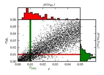
Using the simulations described in §2 and the maximum likelihood method described in §3, we generate realizations of CLASS-like data and infer best-fit parameters from them. The maps all have scalar fluctuations with a fixed normalization () and the same foreground simulation from §2, while the tensor modes have varying strength uniformly sampled with one every . We display a subset of these simulations in Figure 5, marginalized over and the LC coefficients.
Actual CLASS data will provide a maximum likelihood estimate . Using simulated data similar to those from Figure 5, we will estimate the distribution of using the slice . Without knowledge of , however, we need to marginalize over the possible values of that result from cosmic variance given a “true” .
We estimate the constraining power of CLASS prior to a specific measurement . Our goal is to calculate a probability distribution that indicates our best estimate of given some true value, . From simulations, we calculate the probability of a specific value of given a measured , , and the probability of obtaining a given maximum likelihood result given the true value of , . Using this information, we can marginalize over the nuisance parameter, , i.e.
| (6) |
The quantity represents the average of a CLASS-like experiment’s posterior distribution for over many realizations, given that the true amplitude of tensor fluctuations is . This statistic is motivated by noting a single CLASS-like experiment will produce a probability distribution . The random variable is a draw from the distribution , and is not of inherent interest to this discussion. The function acts as a kernel for a weighted average, and is used here to create a weighted average of each , which results in the distribution . We illustrate this process in Figure 5 in which the histogram across the top gives a single realization of and the histogram on the right shows for a specific value for the input model. In this formalism, we can obtain a distribution of expected estimates of given .
We also estimate the constraining power of CLASS’s high-multipole data, with (, ). The model used here has a fixed scalar fluctuation amplitude and spatially constant spectral indices. These simplifications are justified because foreground power spectra decay approximately as , and spurious correlations between the CMB and foregrounds are negligible at these scales (Page et al. 2007; Planck Collaboration 2014). We use an internal linear combination (ILC) method similar to that used in the WMAP analysis (Hinshaw et al. 2007) to clean foregrounds, and then use PolSpice (Chon et al. 2004) to extract the B-mode power spectrum for multipoles . By simulating maps with varying as in the low- simulations, we find that we can describe the likelihood of from the high- distribution with a Gaussian probability distribution with .
This analysis omits multipoles , due to constraints from both the low- and high- software. For the pixel-based approach at low-, the Healpix documentation recommends using to avoid oversampling each pixel, while PolSpice introduces mode-coupling effects in the power spectrum for .
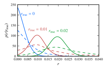
With the distribution for , we obtain the range of potential false positive results, which suggests a definition of our upper limit as the value of that contains 95% of the area under the curve from , yielding for low- data alone, and using the high- simulations as well. Similarly, we estimate the expected range of recovered for , and find that the 68% confidence interval, defined as the percentiles , gives ( including high-). These distributions are displayed in Figure 6. Using a simple likelihood ratio test based on these curves with , we find a likelihood ratio for the low- data with , corresponding to a PTE of , or a significance of . Including high- data gives a projected , corresponding to a PTE of , or a significance of .
5. Conclusions
In this work, we have simulated CMB polarization maps on a cut sky contaminated by diffuse foreground emission and Gaussian white noise. We recovered the input CMB by solving for maximum-likelihood maps using a pixel-based maximum likelihood method tailored to measure the reionization peak (). We have found the following.
-
•
We found unbiased estimates of the amplitudes of scalar and tensor fluctuations with a four-frequency maximum likelihood analysis accounting for CLASS-like noise, a cut sky, and foregrounds with spatially varying spectral indices.
-
•
We have found that, by using only polarization the reionization peak (), data from a five-year CLASS-like experiment would produce a 95% upper limit of , which improves to when we include high- data ().
-
•
Our pixel-based low-multipole maximum likelihood solution is straightforward to run and implement, and is stable to foreground complications, i.e. variable spectral indices and polarization fractions.
Although CLASS’s primary purpose is constraining the amplitude of tensor fluctuations, a foreground-cleaned measurement of CMB polarization on the largest scales can help constrain several other cosmological parameters. Our cosmic variance-limited measurement of the large-scale E-mode power spectrum will improve on the current WMAP and Planck measurements of the optical depth to reionization by a factor of four. Not only can optical depth measurements constrain cosmic reionization scenarios, but it can also further constrain the amplitude of primordial density fluctuations , whose precision is limited by its degeneracy with . With a tightly constrained measurement, comparisons with the amplitude of large scale structure of the Universe, , can be used to infer the sum of neutrino masses to (Allison et al. 2015). Finally, the observed anomalies in the temperature fluctuations on large angular scales require polarization measurements on the same scales to probe physics beyond standard CDM (Bennett et al. 2011; Planck Collaboration 2015d).
Appendix A Signal-to-Noise on Large Angular Scales
The purpose of this Appendix is to demonstrate that in the large-noise limit, the signal-to-noise of B-mode polarization measurements increases with decreasing multipole . Cosmic variance, the uncertainty in the observed CMB anisotropy due to it being a single realization of a Gaussian random field, is a limitation for large scale experiments in particular since the uncertainty in the power spectrum scales as in the cosmic variance limit. For a beam window function and noise power spectrum , the signal-to-noise per multipole of a power spectrum is (Knox 1995)
| (A1) |
For , i.e. in the cosmic variance limit, the factor dominates the signal-to-noise, but when the power spectra of the noise and CMB are comparable the relationship is not as simple, and the projected significance can sometimes increase at large angular scales.
CMB polarization experiments are far from the cosmic variance measurement limits of the B-mode power spectrum, so at large angular scales the signal-to-noise in Equation A1 becomes
| (A2) |
For low multipoles the BB spectrum roughly scales with multipole as , so that signal-to-noise scales as , in contrast with the scaling found in the cosmic variance limit.
Appendix B Dust Spectral Index Variation
The purpose of this Appendix is to demonstrate that the observed variation in dust spectral index observed by Planck (Planck Collaboration 2015f, Planck Int XXII hereafter) is consistent with noise, and does not indicate any intrinsic variation. To estimate the spectral index of thermal dust emission, the Planck team subdivided mid-latitude data into 400 overlapping patches of sky (Planck Int XXII). They subtracted lower frequency data from dust-dominated bands to remove the achromatic CMB component and then took ratios of the residual at two different frequencies, and , denoted
| (B1) | ||||
| (B2) |
where is the spectral index of the dust, is the dust temperature, and is the total signal intensity at frequency . To remove the CMB contribution from the dust-dominated bands, they subtracted from and before taking a ratio, and assumed the dust follows a modified blackbody spectrum . They estimated the dust temperature using with DIRBE data as the high-frequency template, while they computed spectral indices using . Using , they implicitly solved for for each patch.
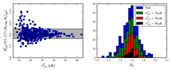
The resulting distribution of from Planck has a dispersion of , which at face value suggests true on-sky spectral index variation. However, each sky patch has an associated local dispersion in the 353 GHz dust template brightness, with higher values corresponding to higher signal-to-noise, and Planck Int XXII claim that low signal-to-noise values with are dominated by instrument noise. Additionally, in Appendix B of Planck Int XXII, Monte Carlo simulations of dust polarization with constant and and instrument noise give a dispersion in (which is therefore entirely due to instrument noise) for sky patches with signal .
Using data from the top plot of Figure 8 of Planck Int XXII and the relation from Equation B2 fixing to be constant, we rescale , assuming a log-linear relation between and . We rescale to have the quoted mean and standard deviation of . We reproduce Figure 8 of Planck Int XXII in our Figure 7. Using these estimates, we compute the standard deviation of subsets of the data with , obtaining , respectively. We observe that the observed variation of for is entirely consistent with effects of instrument noise seen in the Planck Int XXII Monte Carlo simulations and, therefore, with the hypothesis of a constant dust spectral index in the polarization data. Based on this, we claim that our model of dust spatial spectral variation with as shown in Figure 3 is consistent with the latest Planck data.
References
- Aiola et al. (2012) Aiola, S., Amico, G., Battaglia, P., et al. 2012, in Society of Photo-Optical Instrumentation Engineers (SPIE) Conference Series, Vol. 8446, Society of Photo-Optical Instrumentation Engineers (SPIE) Conference Series, 84467A–84467A–12, ADS
- Albrecht & Steinhardt (1982) Albrecht, A., & Steinhardt, P. J. 1982, Physical Review Letters, 48, 1220, ADS
- Allison et al. (2015) Allison, R., Caucal, P., Calabrese, E., Dunkley, J., & Louis, T. 2015, ArXiv e-prints, ADS, 1509.07471
- Appel et al. (2014) Appel, J. W., Ali, A., Amiri, M., et al. 2014, in Society of Photo-Optical Instrumentation Engineers (SPIE) Conference Series, Vol. 9153, Society of Photo-Optical Instrumentation Engineers (SPIE) Conference Series, 91531J–91531J–15, 1408.4789, ADS
- Austermann et al. (2012) Austermann, J. E., Aird, K. A., Beall, J. A., et al. 2012, in Society of Photo-Optical Instrumentation Engineers (SPIE) Conference Series, Vol. 8452, Society of Photo-Optical Instrumentation Engineers (SPIE) Conference Series, 84521E–84521E–18, 1210.4970, ADS
- Bennett et al. (2011) Bennett, C. L., Hill, R. S., Hinshaw, G., et al. 2011, ApJS, 192, 17, ADS, 1001.4758
- Bennett et al. (2013) Bennett, C. L., Larson, D., Weiland, J. L., et al. 2013, ApJS, 208, 20, ADS, 1212.5225
- BICEP2/Keck et al. (2015) BICEP2/Keck, Planck Collaboration, Ade, P. A. R., et al. 2015, Physical Review Letters, 114, 101301, ADS, 1502.00612
- Byrd et al. (1995) Byrd, R. H., Lu, P., Nocedal, J., & Zhu, C. 1995, SIAM J. Sci. Comput., 16, 1190
- Chon et al. (2004) Chon, G., Challinor, A., Prunet, S., Hivon, E., & Szapudi, I. 2004, MNRAS, 350, 914, ADS, astro-ph/0303414
- Chuss et al. (2012) Chuss, D. T., Wollack, E. J., Henry, R., Hui, H., Juarez, A. J., Krejny, M., Moseley, S. H., & Novak, G. 2012, Appl. Opt., 51, 197, ADS, 1106.5984
- Delabrouille et al. (2013) Delabrouille, J., Betoule, M., Melin, J.-B., et al. 2013, A&A, 553, A96, ADS, 1207.3675
- Efstathiou (2006) Efstathiou, G. 2006, MNRAS, 370, 343, ADS, astro-ph/0601107
- Efstathiou et al. (2009) Efstathiou, G., Gratton, S., & Paci, F. 2009, MNRAS, 397, 1355, ADS, 0902.4803
- Eimer et al. (2012) Eimer, J. R., Bennett, C. L., Chuss, D. T., Marriage, T., Wollack, E. J., & Zeng, L. 2012, in Society of Photo-Optical Instrumentation Engineers (SPIE) Conference Series, Vol. 8452, Society of Photo-Optical Instrumentation Engineers (SPIE) Conference Series, 845220–845220–15, 1211.0041, ADS
- Einhorn & Sato (1981) Einhorn, M. B., & Sato, K. 1981, Nuclear Physics B, 180, 385, ADS
- Essinger-Hileman et al. (2014) Essinger-Hileman, T., Ali, A., Amiri, M., et al. 2014, in Society of Photo-Optical Instrumentation Engineers (SPIE) Conference Series, Vol. 9153, Society of Photo-Optical Instrumentation Engineers (SPIE) Conference Series, 91531I–91531I–23, 1408.4788, ADS
- Essinger-Hileman et al. (2010) Essinger-Hileman, T., Appel, J. W., Beall, J. A., et al. 2010, ArXiv e-prints, ADS, 1008.3915
- Filippini et al. (2010) Filippini, J. P., Ade, P. A. R., Amiri, M., et al. 2010, in Society of Photo-Optical Instrumentation Engineers (SPIE) Conference Series, Vol. 7741, Society of Photo-Optical Instrumentation Engineers (SPIE) Conference Series, 77411N–77411N–12, 1106.2158, ADS
- Finkbeiner et al. (1999) Finkbeiner, D. P., Davis, M., & Schlegel, D. J. 1999, ApJ, 524, 867, ADS, astro-ph/9905128
- Fuskeland et al. (2014) Fuskeland, U., Wehus, I. K., Eriksen, H. K., & Næss, S. K. 2014, ApJ, 790, 104, ADS, 1404.5323
- Górski et al. (2005) Górski, K. M., Hivon, E., Banday, A. J., Wandelt, B. D., Hansen, F. K., Reinecke, M., & Bartelmann, M. 2005, ApJ, 622, 759, ADS, astro-ph/0409513
- Guth (1981) Guth, A. H. 1981, Phys. Rev. D, 23, 347, ADS
- Hinshaw et al. (2013) Hinshaw, G., Larson, D., Komatsu, E., et al. 2013, ApJS, 208, 19, ADS, 1212.5226
- Hinshaw et al. (2007) Hinshaw, G., Nolta, M. R., Bennett, C. L., et al. 2007, ApJS, 170, 288, ADS, astro-ph/0603451
- Hu & White (1997) Hu, W., & White, M. 1997, New Astronomy, 2, 323 , astro-ph/9706147
- Kamionkowski et al. (1997) Kamionkowski, M., Kosowsky, A., & Stebbins, A. 1997, Phys. Rev. D, 55, 7368, ADS, astro-ph/9611125
- Katayama & Komatsu (2011) Katayama, N., & Komatsu, E. 2011, ApJ, 737, 78, ADS, 1101.5210
- Kazanas (1980) Kazanas, D. 1980, ApJ, 241, L59, ADS
- Kermish et al. (2012) Kermish, Z. D., Ade, P., Anthony, A., et al. 2012, in Society of Photo-Optical Instrumentation Engineers (SPIE) Conference Series, Vol. 8452, Society of Photo-Optical Instrumentation Engineers (SPIE) Conference Series, 84521C–84521C–15, 1210.7768, ADS
- Knox (1995) Knox, L. 1995, Phys. Rev. D, 52, 4307, ADS, astro-ph/9504054
- Lazear et al. (2014) Lazear, J., Ade, P. A. R., Benford, D., et al. 2014, 9153, 91531L, ADS, 1407.2584
- Linde (1982) Linde, A. D. 1982, Physics Letters B, 108, 389, ADS
- López-Caniego et al. (2014) López-Caniego, M., Rebolo, R., Aguiar, M., et al. 2014, ArXiv e-prints, ADS, 1401.4690
- Miller et al. (2015) Miller, N. J., Chuss, D. T., Marriage, T. A., et al. 2015, ArXiv e-prints, ADS, 1509.04628
- Miville-Deschênes et al. (2008) Miville-Deschênes, M.-A., Ysard, N., Lavabre, A., Ponthieu, N., Macías-Pérez, J. F., Aumont, J., & Bernard, J. P. 2008, A&A, 490, 1093, ADS, 0802.3345
- Mukhanov & Chibisov (1981) Mukhanov, V. F., & Chibisov, G. V. 1981, Soviet Journal of Experimental and Theoretical Physics Letters, 33, 532, ADS
- Niemack et al. (2010) Niemack, M. D., Ade, P. A. R., Aguirre, J., et al. 2010, in Society of Photo-Optical Instrumentation Engineers (SPIE) Conference Series, Vol. 7741, Society of Photo-Optical Instrumentation Engineers (SPIE) Conference Series, 77411S–77411S–21, 1006.5049, ADS
- Ogburn et al. (2010) Ogburn, IV, R. W., Ade, P. A. R., Aikin, R. W., et al. 2010, in Society of Photo-Optical Instrumentation Engineers (SPIE) Conference Series, Vol. 7741, Society of Photo-Optical Instrumentation Engineers (SPIE) Conference Series, 77411G–77411G–11, ADS
- Oxley et al. (2004) Oxley, P., Ade, P. A., Baccigalupi, C., et al. 2004, in Society of Photo-Optical Instrumentation Engineers (SPIE) Conference Series, Vol. 5543, Infrared Spaceborne Remote Sensing XII, ed. M. Strojnik, 320–331, astro-ph/0501111, ADS
- Page et al. (2007) Page, L., Hinshaw, G., Komatsu, E., et al. 2007, ApJS, 170, 335, ADS, astro-ph/0603450
- Planck Collaboration (2014) Planck Collaboration. 2014, ArXiv e-prints, ADS, 1409.5738
- Planck Collaboration (2015a) —. 2015a, ArXiv e-prints, ADS, 1502.01582
- Planck Collaboration (2015b) —. 2015b, ArXiv e-prints, ADS, 1502.01588
- Planck Collaboration (2015c) —. 2015c, ArXiv e-prints, ADS, 1502.01589
- Planck Collaboration (2015d) —. 2015d, ArXiv e-prints, ADS, 1506.07135
- Planck Collaboration (2015e) —. 2015e, ArXiv e-prints, ADS, 1502.02114
- Planck Collaboration (2015f) —. 2015f, A&A, 576, A107, ADS, 1405.0874
- Polnarev (1985) Polnarev, A. G. 1985, Soviet Ast., 62, 1041, ADS
- Rostem et al. (2014) Rostem, K., Ali, A., & Appel, J. W. o. 2014, in Society of Photo-Optical Instrumentation Engineers (SPIE) Conference Series, Vol. 9153, Society of Photo-Optical Instrumentation Engineers (SPIE) Conference Series, 91530B–91530B–7, 1408.4790, ADS
- Seljak & Zaldarriaga (1997) Seljak, U., & Zaldarriaga, M. 1997, Physical Review Letters, 78, 2054, ADS, astro-ph/9609169
- Starobinsky (1980) Starobinsky, A. A. 1980, Physics Letters B, 91, 99, ADS
- Tajima et al. (2012) Tajima, O., Choi, J., Hazumi, M., Ishitsuka, H., Kawai, M., & Yoshida, M. 2012, in Society of Photo-Optical Instrumentation Engineers (SPIE) Conference Series, Vol. 8452, Society of Photo-Optical Instrumentation Engineers (SPIE) Conference Series, 84521M–84521M–9, ADS